Discrete conservation laws for finite element discretisations of multisymplectic PDEs

Abstract.

In this work we propose a new, arbitrary order space-time finite element discretisation for Hamiltonian PDEs in multisymplectic formulation. We show that the new method which is obtained by using both continuous and discontinuous discretisations in space, admits a local and global conservation law of energy. We also show existence and uniqueness of solutions of the discrete equations. Further, we illustrate the error behaviour and the conservation properties of the proposed discretisation in extensive numerical experiments on the linear and nonlinear wave equation and on the nonlinear Schrödinger equation.

1. Introduction

Finite element discretisations of space-time variational problems have seen a revival of interest in the recent literature [35, 46, 1, 53], with their origin going back to the work of [37, 3]. The focus of the present work is the structure-preserving discretisation of variational problems using finite element methods. The point of departure is the variational space-time formulation of PDE problems arising as the Euler-Lagrange equations of a space-time action functional. Formally via the Legendre transform one obtains the Hamiltonian formulation of these partial differential equations [45]. However a space-time analogue of the Legendre transform gives rise to the so called multisymplectic formulation of these PDEs as originally proposed by Bridges [9], and intrinsically generalised in [39, 38].

There are two main proposed discretisation approaches to the multisymplectic formulation of Hamiltonian PDEs. The first is inspired by a technique proposed by Veselov to discretise Hamiltonian ODEs and consists of discretising the Lagrangian density to yield a discrete analogue of the variational principle, and then extremising to obtain discrete Euler Lagrange equations, [38]. The second is obtained by first extremising the variational principle, writing the multisymplectic PDEs in the strong multisymplectic formulation, and then discretising these equations with structure preserving approximations, [10]. The first approach leads automatically to the conservation of a discrete multisymplectic conservation law and the corresponding numerical methods typically show as a side effect good local conservation of a modified energy and momentum in numerical experiments. The second approach is more flexible, while discretisations with similar properties can be obtained using appropriate multisymplectic schemes [10], this formulation can be also easily adopted to obtain methods satisfying local conservation laws of energy or momentum [28]. In the sequel we shall follow the latter approach. We note for Hamiltonian ODEs that symplectic schemes are often preferred over conservative schemes as they allow for backward error analysis, and the resulting schemes will preserve a modified conserved quantity [29]. A backward error analysis for multisymplectic schemes in the PDE setting is not yet fully developed, [44, 32]. On the other hand, being able to bound the approximation by the energy often proves to be an invaluable property for convergence studies of both geometric numerical integrators [21, 12, 11] and finite element schemes via energy arguments [52].

Most of the proposed discretisations of multisymplectic PDEs are proposed in the framework of finite differences with restrictions to rectangular domains, are not easy to use on irregular domains, and are often of low order with some exceptions [56, 51, 43, 48, 42, 5]. Due to the nature of their formulation, finite element methods may overcome these issues. It has also been remarked [49] that some of the proposed multisymplectic discretisations might not be well defined locally and or globally or not have solutions/unique solutions, [2], [42].

Standard finite element methods, when arising from boundary value problems, do not historically lead to discretisations which may be interpreted locally. Indeed, we may on a case-by-case basis move out of the finite element framework through the assembling of the associated algebraic system which may then be interpreted locally similarly to a spatial finite difference discretisation, see for example [36]. The recent work [43] utilises the hybridisable discontinuous Galerkin framework [18], in which the solution inside an element and on the element boundaries are considered independently and coupled to ensure global communication of the solution. Fortuitously, standard finite element methods also fit within this framework [19], and as such global solution properties may be naturally restricted to the patch surrounding a single element.

Another novel approach which allows for the incorporation of spatially local conservation laws are local discontinuous Galerkin (ldG) methods [20, 15, 55], in which a given PDE is reduced to a first order system through the incorporation of auxiliary variables. The resulting discretisation is comprised of discontinuous approximations of first derivatives utilising either upwind or downwind flux contributions, which allow for the development of schemes which preserve conservation laws for PDEs with even order spatial derivatives [54, 16]. A crucial implementational benefit of these methods is that due to the discontinuous nature of the approximation the discrete system may be rewritten as a single equation, and as such the resulting algorithms are of a competitive complexity. In this work, we shall consider similar spatial discretisations, however, due to the general multisymplectic framework considered we choose an average spatial flux, as opposed to the upwind/downwind considered in the ldG setting. Our choice here is similar to that made in [34]. This average spatial flux choice allows us to utilise a discrete integration by parts which is fundamental to the preservation of conservation laws in a general setting. If we restrict ourselves to consider multisymplectic PDEs with even order spatial derivatives, appropriate modifications of the spatial derivative may be designed to preserve local conservation laws for this class of multisymplectic PDEs with upwind/downwind fluxes, which often yields an optimal rate of convergence in the resulting numerical scheme.

Temporally, finite element methods are a competitive, well studied, class of methods [23, 25, 22] dating back to 1969 [26]. Further to this, the conforming approximation is well known to preserve energy for Hamiltonian problems [7, 30, 50, 33]. For space-time finite element approximations the temporal are typically nonconforming, with the standard choice of a discontinuous upwind flux introducing artificial diffusion [24] which facilitates stability, even when the space-time algorithm is adapted. Here we shall focus our attention on the temporally conforming approximation, with a view to extend this work to incorporate a new form of conservative space-time adaptive algorithm with inherent stability building on ideas developed in [33].

The outline of the paper is as follows, in Section 2 we briefly review the main features of multisymplectic PDEs including examples; in Section 3 we present the continuous space-time finite element discretisation and prove existence and uniqueness of solutions of the discrete equations at the end of the section; in Section 4 we extend the method to the spatially discontinuous case; in Section 5 we conduct numerical experiments; and in Section 6 we conclude.

2. Multisymplectic PDEs

Let $u=u(t,x)$ where $t\in[0,T]$ and $x\in S^{1}=[0,1)$ periodic and consider the space-time variational problem

$$0=\delta\int_{[0,T]\times S^{1}}L(u,u_{t},u_{x})\,\text{ }\mathrm{d}{x}\,\text{ }\mathrm{d}{t},$$ (2.1)

where $L(u,u_{t},u_{x})$ is some given Lagrangian density function. Multisymplectic PDEs may arise naturally from such problems through the following methodology. Introducing the auxiliary variables

$$v:=\frac{\partial L}{\partial u_{t}},\qquad w:=\frac{\partial L}{\partial u_{x}},$$

and assuming that $u_{t}=u_{t}(v),$ $u_{x}=u_{x}(w)$ are invertible functions, we can define the Hamiltonian density

$$\mathcal{S}\left(u,v,w\right):=vu_{t}+wu_{x}-L(u,u_{t}(v),u_{x}(w)).$$

We may then express the variational principle by means of $\mathcal{S}\left(u,v,w\right)$ in the new variables as

$$0=\delta\int_{[0,T]\times S^{1}}\left(vu_{t}+wu_{x}-\mathcal{S}\left(u,v,w\right)\right)\,\text{ }\mathrm{d}{x}\,\text{ }\mathrm{d}{t},$$

and through taking variations $\left(\psi_{u},\psi_{v},\psi_{w}\right)^{T}=:\boldsymbol{\psi}$ we obtain

$$0=\int_{[0,T]\times S^{1}}\left(K\,\boldsymbol{z}_{t}+L\,\boldsymbol{z}_{x}-\nabla\mathcal{S}\left(\boldsymbol{z}\right)\right)\cdot\boldsymbol{\psi}\quad\text{ }\mathrm{d}{x}\,\text{ }\mathrm{d}{t},\qquad\forall\boldsymbol{\psi},$$ (2.2)

where

$$\boldsymbol{z}:=\left[\begin{array}[]{c}u\\ v\\ w\end{array}\right],\quad\boldsymbol{\psi}:=\left[\begin{array}[]{c}\psi_{u}\\ \psi_{v}\\ \psi_{w}\end{array}\right],\qquad K=\left[\begin{array}[]{ccc}0&-1&0\\ 1&0&0\\ 0&0&0\end{array}\right],\qquad L=\left[\begin{array}[]{ccc}0&0&-1\\ 0&0&0\\ 1&0&0\end{array}\right].$$

We note that this integral yields an example of what we refer to as a multisymplectic PDE as discussed in [9], and includes examples such as wave equations. Additionally, through modifying the dependencies of the Lagrangian density function we may obtain more examples of multisymplectic PDEs. This underlying variational nature of multisymplectic PDEs advocates space-time finite elements as a desirable discretisation methodology.

Definition 2.1 (Multisymplectic PDEs).

Let $t\in[0,T]$ for some fixed $T$ and let $x\in S^{1}:=[0,1)$ be periodic. Further let $K,L\in{}^{D\times D}$ be constant skew-symmetric matrices for integer $D\geq 2$. Then a multisymplectic PDE is described by seeking $\boldsymbol{z}:(t,x)\to{}^{D}$ such that

$$K\boldsymbol{z}_{t}+L\boldsymbol{z}_{x}=\nabla\mathcal{S}\left(\boldsymbol{z}\right),$$ (2.3)

where $\mathcal{S}:{}^{D}\to\real$.

Remark 2.2 (Skew-symmetric inner product).

A skew-symmetric matrix induces a skew-symmetric product, that is to say that if we have $\boldsymbol{u},\boldsymbol{v}\in{}^{D}$ then for any skew-symmetric $K\in{}^{D\times D}$

$$\boldsymbol{u}\cdot K\boldsymbol{v}=-K\boldsymbol{u}\cdot\boldsymbol{v},$$ (2.4)

where $\cdot$ denotes the Euclidean inner product.

The namesake of a multisymplectic PDE is its multisymplectic structure, which falls within the form of a conservation law. To fully describe this structure we utilise the Cartan derivative and the skew-symmetric wedge product. For a detailed analysis of the multisymplectic structure see [10].

Theorem 2.3 (Multisymplectic structure).

The PDE (2.3) possesses the multisymplectic conservation law

$$\left(\,\mathrm{d}\boldsymbol{z}\wedge K\boldsymbol{z}\right)_{t}+\left(\,\mathrm{d}\boldsymbol{z}\wedge L\boldsymbol{z}\right)_{x}=0.$$ (2.5)

Proof.

Applying the Cartan exterior derivative to (2.3) we find

$$K\,\mathrm{d}\boldsymbol{z}_{t}+L\,\mathrm{d}\boldsymbol{z}_{x}=\nabla^{T}\nabla\mathcal{S}\left(\boldsymbol{z}\right)\,\mathrm{d}\boldsymbol{z}.$$ (2.6)

Acting on (2.6) with $\wedge\,\mathrm{d}\boldsymbol{z}$ from the right we can write

$$K\,\mathrm{d}\boldsymbol{z}_{t}\wedge\,\mathrm{d}\boldsymbol{z}+L\,\mathrm{d}\boldsymbol{z}_{x}\wedge\,\mathrm{d}\boldsymbol{z}=\nabla^{T}\nabla\mathcal{S}\left(\boldsymbol{z}\right)\,\mathrm{d}\boldsymbol{z}\wedge\,\mathrm{d}\boldsymbol{z}.$$ (2.7)

Through the skew-symmetry of the wedge product we find that

$$\frac{1}{2}\left(K\,\mathrm{d}\boldsymbol{z}\wedge\boldsymbol{z}\right)_{t}=K\,\mathrm{d}\boldsymbol{z}_{t}\wedge\,\mathrm{d}\boldsymbol{z},$$ (2.8)

and similarly for the spatial derivative. Additionally, through the skew-symmetry of the wedge product and the symmetry of $\nabla^{T}\nabla\mathcal{S}\left(\boldsymbol{z}\right)$ we have that

$$\nabla^{T}\nabla\mathcal{S}\left(\boldsymbol{z}\right)\,\mathrm{d}\boldsymbol{z}\wedge\,\mathrm{d}\boldsymbol{z}=0,$$ (2.9)

allowing us to conclude.

∎

Remark 2.4 (The discrete preservation of the multisymplectic structure).

The multisymplectic structure discussed in Theorem 2.3 is possible to preserve on the discrete level, and leads to desirable numerical results, see [10, 43, 40, 13, 5].

On a fundamental level, multisymplectic conservation laws treat time and space equivalently, which is natural for elliptic and some hyperbolic problems. However, for evolution problems this is not always ideal. Indeed, even boundary conditions are treated independently in space and time. In this contribution we shall discretise space and time non-homogeneously, in the sense that our discretisations in each variable are fundamentally different. Indeed, in the lowest order conforming case our proposed discretisation will be equivalent to discretising with the Average Vector Field method in time and conforming finite elements in space [17]. As such, we do not expect the methods proposed here to exactly preserve a discrete multisymplectic conservation law.

Further to the multisymplectic conservation laws, all multisymplectic PDEs also preserve momentum and energy conservation laws, which correspond to spatial and temporal translations respectively via Noether’s theorem.

Theorem 2.5 (Classical conservation laws in multisymplectic PDEs).

Let $\boldsymbol{z}$ be the solution of the multisymplectic PDE (2.3) as set out in Definition (2.1). Further define the momentum flux and density as

$${F}^{1}=\frac{1}{2}\boldsymbol{z}\cdot K\boldsymbol{z}_{t}-\mathcal{S}\left(\boldsymbol{z}\right)\qquad\qquad{D}^{1}=\frac{1}{2}\boldsymbol{z}_{x}\cdot K\boldsymbol{z}$$ (2.10)

respectively, and energy flux and density as

$${F}^{2}=\frac{1}{2}\boldsymbol{z}_{t}\cdot L\boldsymbol{z}\qquad\qquad{D}^{2}=\frac{1}{2}\boldsymbol{z}\cdot L\boldsymbol{z}_{x}-\mathcal{S}\left(\boldsymbol{z}\right)$$ (2.11)

respectively. Then the momentum conservation law

$${D}^{1}_{t}+{F}^{1}_{x}=0$$ (2.12)

holds. Additionally, $\boldsymbol{z}$ possesses the energy conservation law

$${D}^{2}_{t}+{F}^{2}_{x}=0.$$ (2.13)

Proof.

The proofs of (2.12) and (2.13) follow from the application of the PDE (2.3) and the constant skew-symmetric structures of the $K$ and $L$. As we utilise this methodology for the proof of momentum and energy conservation laws on the discrete level we shall present the proof of (2.12) fully to inform the sequel.

Through (2.10) we can write

$${F}^{1}_{x}=\frac{1}{2}\boldsymbol{z}_{x}\cdot K\boldsymbol{z}_{t}+\frac{1}{2}\boldsymbol{z}\cdot K\boldsymbol{z}_{tx}-\nabla\mathcal{S}\left(\boldsymbol{z}\right)\cdot\boldsymbol{z}_{x}.$$ (2.14)

Acting on the PDE (2.3) with $\cdot\boldsymbol{z}_{x}$ from the right we have

$$\nabla\mathcal{S}\left(\boldsymbol{z}\right)\cdot\boldsymbol{z}_{x}=K\boldsymbol{z}_{t}\cdot\boldsymbol{z}_{x}+L\boldsymbol{z}_{x}\cdot\boldsymbol{z}_{x}=K\boldsymbol{z}_{t}\cdot\boldsymbol{z}_{x},$$ (2.15)

through the skew-symmetry of $L$. Applying (2.15) to (2.14) we find

$${F}^{1}_{x}=-\frac{1}{2}\boldsymbol{z}_{x}\cdot K\boldsymbol{z}_{t}+\frac{1}{2}\boldsymbol{z}\cdot K\boldsymbol{z}_{tx}.$$ (2.16)

Through (2.10) we can also write

$$\begin{split}{D}^{1}_{t}&=\frac{1}{2}\boldsymbol{z}_{xt}\cdot K\boldsymbol{z}+\frac{1}{2}\boldsymbol{z}_{x}\cdot K\boldsymbol{z}_{t}\\ &=-\frac{1}{2}\boldsymbol{z}\cdot K\boldsymbol{z}_{xt}+\frac{1}{2}\boldsymbol{z}_{x}\cdot K\boldsymbol{z}_{t},\end{split}$$ (2.17)

through the skew-symmetry of $K$. Summing (2.16) and (2.17) we obtain the desired result for the momentum law (2.12). For the energy law (2.13) we follow the same methodology but instead act on (2.3) with $\cdot\boldsymbol{z}_{t}$.

∎

Example 2.6 (Nonlinear wave equations).

Consider the nonlinear wave equation

$$u_{tt}-u_{xx}-\mathcal{V}^{\prime}(u)=0.$$ (2.18)

Through the introduction of the auxiliary variables

$$\begin{split}v&:=u_{t}\\ w&:=u_{x},\end{split}$$ (2.19)

we can write the nonlinear wave equation in multisymplectic form through defining $\boldsymbol{z}=(u,v,w)$, so $D=3$, with

$$\begin{split}K=\begin{pmatrix}0&-1&0\\ 1&0&0\\ 0&0&0\end{pmatrix}&\qquad\qquad\qquad L=\begin{pmatrix}0&0&1\\ 0&0&0\\ -1&0&0\end{pmatrix}\\ \mathcal{S}\left(\boldsymbol{z}\right)&=\frac{1}{2}v^{2}-\frac{1}{2}w^{2}+\mathcal{V}(u).\end{split}$$ (2.20)

We additionally observe that the multisymplectic form of the momentum and energy density are compatible with the standard forms which are given by $\frac{1}{2}u_{xt}u-\frac{1}{2}u_{x}u_{t}$ and $\frac{1}{2}uu_{xx}-\frac{1}{2}u_{t}^{2}-\mathcal{V}(u)$ respectively. Note that this multisymplectic PDE falls within the framework discussed at the beginning of this section, with a Lagrangian density of

$$L\left(u,u_{t},u_{x}\right)=\frac{1}{2}u_{t}^{2}-\frac{1}{2}u_{x}^{2}-\mathcal{V}(u).$$ (2.21)

Example 2.7 (A nonlinear Schrödinger equation).

Let us consider the nonlinear Schrödinger (NLS) equation

$$i\xi_{t}+\xi_{xx}+\left|\xi\right|^{2}\xi=0,$$ (2.22)

where $\xi(t,x)$ takes complex values. Through splitting into real and complex components, and introducing auxiliary variables for the spatial derivatives, we may rewrite the NLS equation in multisymplectic form. In particular, we define $\boldsymbol{z}=(u,v,p,q)$ through the introduction of the variables

$$\begin{split}u&=\mathrm{Re}\left(\xi\right)\\ v&=\mathrm{Im}\left(\xi\right)\\ p&=u_{x}\\ q&=v_{x},\end{split}$$ (2.23)

the multisymplectic formulation may then be expressed through the skew-symmetric operators

$$\begin{split}K=\begin{pmatrix}0&-1&0&0\\ 1&0&0&0\\ 0&0&0&0\\ 0&0&0&0\end{pmatrix}&\qquad\qquad\qquad L=\begin{pmatrix}0&0&1&0\\ 0&0&0&1\\ -1&0&0&0\\ 0&-1&0&0\end{pmatrix},\end{split}$$ (2.24)

and the symmetric nonlinear function

$$\mathcal{S}\left(\boldsymbol{z}\right)=-\frac{1}{4}\left(u^{2}+v^{2}\right)^{2}-\frac{1}{2}\left(p^{2}+q^{2}\right).$$ (2.25)

3. Continuous space-time finite element approximations

We shall now focus on the design of a conforming space-time finite element method which is constructed through the tensor product of spatial and temporal finite element discretisations. This decoupling of the spatial and temporal discretisations allows us to combine a conservative spatial method with a temporally conservative method, which for the study of Hamiltonian ODEs and Hamiltonian PDEs are fundamentally different, see [33].

Before defining our finite element space we must give consideration to the discretisation of the temporal and spatial domains. We partition our temporal domain $\left[0,T\right]$ such that $0:=t_{0}<t_{1}<\cdots<t_{N}=:T$, and define a temporal finite element as $\mathcal{I}_{n}:=\left[t_{n},t_{n+1}\right)$ which possesses an element length $\tau_{n}:=t_{n+1}-t_{n}$. Similarly, we partition our periodic spatial domain $S^{1}$ such that $0:=x_{0}<x_{1}<\cdots<x_{M}:=1$ and define a spatial finite element as $\mathcal{J}_{m}:=\left(x_{m},x_{m+1}\right)$ which possesses an element length $h_{m}:=x_{m+1}-x_{m}$.

To define the spatial and temporal finite element spaces simultaneously we consider an arbitrary domain $\Omega\subset\real$ which is partitioned such that $y_{0}<y_{1}<\cdots<y_{J}$ possessing an arbitrary element $\mathcal{K}_{j}:=\left(y_{j},y_{j+1}\right)$.

Definition 3.1 (Finite element spaces).

The concise definition of a given finite element space depends on the discretisation of the domain being considered. Here we consider the discretisation of $\Omega$ by the elements $\mathcal{K}_{j}$.

Let $\mathbb{P}_{r}\left(\mathcal{K}_{j}\right)$ denote the space of polynomials of degree $r$ on an interval $\mathcal{K}_{j}\subset\mathbb{R}$, and $\left(\mathbb{P}_{r}\left(\mathcal{K}_{j}\right)\right)^{D}$ be the $D$-dimensional vector extension of the aforementioned space, then the discontinuous finite element space is

$$\mathbb{V}_{r}\left(\Omega\right)=\{\boldsymbol{W}:\left.\boldsymbol{W}\right|_{\mathcal{K}_{j}}\in\left(\mathbb{P}_{r}\left(\mathcal{K}_{j}\right)\right)^{D},j=0,...,J-1\},$$ (3.1)

further to this the continuous finite element space is defined analogously with global continuity enforced, i.e.,

$$\mathbb{V}_{r}^{C}(\Omega)=\mathbb{V}_{r}(\Omega)\cap\left(\mathcal{C}^{0}\left(\Omega\right)\right)^{D}.$$ (3.2)

Remark 3.2 (Space-time finite element space).

In this work we define our space-time finite element spaces through the tensor product of one dimensional temporal and spatial finite element spaces, allowing us, in some sense, to use temporal or spatial finite element techniques where required. We shall seek a discrete solution in the trial space

$$\mathbb{V}_{q+1}^{C}\left(\left[0,T\right]\right)\times\mathbb{V}_{p}^{C}\left(S^{1}\right)$$ (3.3)

which we test against all functions in

$$\mathbb{V}_{q}\left(\left[0,T\right]\right)\times\mathbb{V}_{p}^{C}\left(S^{1}\right).$$ (3.4)

Note that spatially we choose our trial and test spaces to be the same, however, temporally we choose our trial space such that if we differentiate in time we enter the test space. This is typical for conservative temporal finite element approximations, see [50, 7, 30, 23, 8, 33]. Both the spatial and temporal spaces for the trial functions are conforming, in the sense that they are finite dimensional subspaces of the solution space on the continuous level.

We may define our space-time finite element approximation of multisymplectic PDEs as follows.

Definition 3.3 (Continuous space-time finite element method).

Seek $\boldsymbol{Z}\in\mathbb{V}_{q+1}^{C}\left(\left[0,T\right]\right)\times\mathbb{V}_{p}^{C}\left(S^{1}\right)$ such that

$$\begin{split}\int_{\left[0,T\right]\times S^{1}}K\boldsymbol{Z}_{t}\cdot\phi+L\boldsymbol{Z}_{x}\cdot\phi-\nabla\mathcal{S}\left(\boldsymbol{Z}\right)\cdot\phi\text{ }\mathrm{d}{x}\text{ }\mathrm{d}{t}&=0\qquad\forall\phi\in\mathbb{V}_{q}\left(\left[0,T\right]\right)\times\mathbb{V}_{p}^{C}\left(S^{1}\right)\\ \boldsymbol{Z}(0,x)&=\Pi_{0}\left(\boldsymbol{z}(0,x)\right),\end{split}$$ (3.5)

where $\Pi_{0}$ represents the $L_{2}$ projection into $\mathbb{V}_{p}^{C}(S^{1})$.

Remark 3.4 (Localisation of the finite element method).

While we have formulated (3.5) globally, it is crucial that we can write the formulation locally in time due to the evolutionary nature of the problem. By design, our test function $\phi$ is discontinuous which allows us to rewrite the method in a time stepping fashion as seeking $\boldsymbol{Z}\in\mathbb{V}_{q+1}^{C}\left(\mathcal{I}_{n}\right)\times\mathbb{V}_{p}\left(S^{1}\right)$ for $n=0,...,N-1$ such that

$$\begin{split}\int_{\mathcal{I}_{n}\times S^{1}}K\boldsymbol{Z}_{t}\cdot\psi+L\boldsymbol{Z}_{x}\cdot\psi-\nabla\mathcal{S}\left(\boldsymbol{Z}\right)\cdot\psi\text{ }\mathrm{d}{x}\text{ }\mathrm{d}{t}&=0\qquad\forall\psi\in\mathbb{P}_{q}\left(\mathcal{I}_{n}\right)\times\mathbb{V}_{p}\left(S^{1}\right),\end{split}$$ (3.6)

where $\boldsymbol{Z}(t_{n},x)$ is enforced through either global continuity, or the initial condition $\boldsymbol{Z}(0,x)=\Pi_{0}\left(\boldsymbol{z}(0,x)\right)$. This local formulation can be implemented in a time stepping fashion.

Further to localising time we may localise the formulation over space. However, as the test functions are spatially continuous we may not express this localisation concisely, without the incorporation of hybridisable dG techniques or through examining the underlying nonlinear system of equations for which we solve.

Remark 3.5 (A spatially discontinuous finite element approximation).

To clarify exposition here we have assumed a spatially continuous finite element approximation. In fact, through an appropriate discretisation of the spatial derivative we may construct a discontinuous geometric space-time finite element discretisation. A discontinuous discretisation has two significant benefits: The first is the resulting method is more receptive to adaptivity due to the spatially discontinuous nature of the solution, although complications do arise from the temporal continuity. The second is that the discontinuous nature allows us to employ local discontinuous Galerkin techniques [20] to reduce the dimension of the system within the implementation of the method through rewriting the method as a single equation in terms of the original variable. This is often referred to as the primal form [14]. In practice, this is standard for the implementation of multisymplectic PDEs, such as box schemes [10, 2]. We note that due to the conforming nature of the finite element method in time, we still cannot reduce components of the system with temporal derivatives into primal form. The development of novel tools is required to design a fully discontinuous approximation and falls beyond the scope of this work, although progress has been made to these ends [33, Chapter 3]. We shall investigate a spatially discontinuous approximation in detail in Section 4.

We shall now investigate the discrete conservation laws which are preserved by continuous space-time finite element approximation.

Theorem 3.6 (Discrete conservation laws).

Let the conditions of Definition (3.3) hold, and in particular let $\boldsymbol{Z}$ be the solution of the space-time finite element method (3.5). Additionally define the scalar function

$$W:=\nabla\mathcal{S}\left(\boldsymbol{Z}\right)\cdot\Pi\left(\boldsymbol{Z}_{x}\right),$$ (3.7)

where $\Pi$ is the $L_{2}$ projection into the finite element space $\mathbb{V}_{q}\left(\mathcal{I}_{n}\right)\times\mathbb{V}_{p}^{C}\left(S^{1}\right)$. Further define the fluxes $\varmathbb{F}^{1},\varmathbb{F}^{2}$ and densities $\varmathbb{D}^{1},\varmathbb{D}^{2}$ such that

$$\varmathbb{F}^{1}=\frac{1}{2}\boldsymbol{Z}_{t}\cdot K\boldsymbol{Z}-\mathcal{S}\left(\boldsymbol{Z}\right)\quad \quad\varmathbb{D}^{1}=\frac{1}{2}\boldsymbol{Z}_{x}\cdot K\boldsymbol{Z}$$ (3.8)

$$\varmathbb{F}^{2}=\frac{1}{2}\boldsymbol{Z}_{t}\cdot L\boldsymbol{Z}\quad \quad\varmathbb{D}^{2}=\frac{1}{2}\boldsymbol{Z}_{x}\cdot L\boldsymbol{Z}-\mathcal{S}\left(\boldsymbol{Z}\right).$$ (3.9)

The numerical solution $\boldsymbol{Z}$ conserves a consistent discrete momentum locally in time, namely

$$\int_{\mathcal{I}_{n}\times S^{1}}{\varmathbb{D}^{1}}_{t}+\left(\varmathbb{F}^{1}+\mathcal{S}\left(\boldsymbol{Z}\right)\right)_{x}-W\text{ }\mathrm{d}{x}\text{ }\mathrm{d}{t}=0.$$ (3.10)

Additionally, a discrete energy is conserved locally in time, which we can write as

$$\int_{\mathcal{I}_{n}\times S^{1}}\varmathbb{D}^{2}_{t}+\varmathbb{F}^{2}_{x}\text{ }\mathrm{d}{x}\text{ }\mathrm{d}{t}=0.$$ (3.11)

Remark 3.7 (Initial remarks on Theorem 3.6).

$W$ as constructed in (3.7) is a discrete approximation of $\mathcal{S}\left(\boldsymbol{Z}\right)$, which is designed to allow us to apply the finite element approximation to the spatial momentum flux contribution in a way which mimics the continuous arguments. This construction is required as $\boldsymbol{Z}_{x}$ is not in the test space due to the Petrov-Galerkin nature of the formulation in time and the global continuity of the spatial finite element space.

As our method is constructed under spatial and temporal integrals, the natural discrete conservation laws must also be defined under the integral. This weakens the notion of a conservation law. This may be strengthened slightly when considering a spatially discontinuous approximation by explicitly localising these laws to single elements in space-time, as will be seen in Section 4.

Remark 3.8 (The consistent conserved momentum described in Theorem 3.6).

We note that the consistent discrete momentum conservation (3.10) law does not fall concisely within the expected format for a conservation law. The lack of conservation here is caused by the typically nonlinear term $\nabla\mathcal{S}\left(\boldsymbol{Z}\right)$ and the fact that $Z_{x}$ does not live within the finite element space $\mathbb{V}_{q}\left(\mathcal{I}_{n}\right)\times\mathbb{V}_{p}^{C}\left(S^{1}\right)$. On a case by case basis, the conservation of momentum may be examined for particular examples. We shall see that in situations where schemes have been constructed in the literature which preserve both invariants, we also may expect conservation of both momentum and energy, for example for the linear wave equation, we do indeed obtain it. For brevity we shall not present proofs on a case by case basis here instead presenting select numerical simulations.

In cases where we do not obtain a momentum conservation law through alternate means, we note that the deviation in momentum may be quantified locally by

$$\int_{\mathcal{I}_{n}\times S^{1}}\mathcal{S}\left(\boldsymbol{Z}\right)_{x}-\nabla\mathcal{S}\left(\boldsymbol{Z}\right)\cdot\Pi\left(\boldsymbol{Z}_{x}\right)\text{ }\mathrm{d}{x}\text{ }\mathrm{d}{t},$$ (3.12)

which may be written equivalently as

$$\int_{\mathcal{I}_{n}\times S^{1}}\nabla\mathcal{S}\left(\boldsymbol{Z}\right)\cdot\left(\boldsymbol{Z}_{x}-\Pi\left(\boldsymbol{Z}_{x}\right)\right)\text{ }\mathrm{d}{x}\text{ }\mathrm{d}{t},$$ (3.13)

so the deviation in momentum is quantified by the difference between $\boldsymbol{Z}_{x}$ and its projection into the finite element space. This may be thought of as a quantification of how discontinuous the spatial derivative of $\boldsymbol{Z}$ is. Experimentally, when simulating smooth solutions which are not highly oscillatory we expect this deviation to be small.

Proof of Theorem 3.6.

Through the definition of the momentum density $\varmathbb{D}^{1}$ given in (3.8) we can write

$$\begin{split}\int_{\mathcal{I}_{n}\times S^{1}}{\varmathbb{D}^{1}}_{t}\text{ }\mathrm{d}{x}\text{ }\mathrm{d}{t}&=\int_{\mathcal{I}_{n}\times S^{1}}\frac{1}{2}\boldsymbol{Z}_{xt}\cdot K\boldsymbol{Z}\ +\ \frac{1}{2}\boldsymbol{Z}_{x}\cdot K\boldsymbol{Z}_{t}\ \text{ }\mathrm{d}{x}\text{ }\mathrm{d}{t}\\ &\ =\int_{\mathcal{I}_{n}\times S^{1}}\boldsymbol{Z}_{x}\cdot K\boldsymbol{Z}_{t}\text{ }\mathrm{d}{x}\text{ }\mathrm{d}{t},\end{split}$$ (3.14)

in view of the skew-symmetric inner product induced by $K$ and integration by parts. Further, through the definition of the momentum flux $\varmathbb{F}^{1}$ in (3.8) we find

$$\begin{split}\int_{\mathcal{I}_{n}\times S^{1}}\left({\varmathbb{F}^{1}}+\mathcal{S}\left(\boldsymbol{Z}\right)\right)_{x}-W\text{ }\mathrm{d}{x}\text{ }\mathrm{d}{t}&=\int_{\mathcal{I}_{n}\times S^{1}}-\nabla\mathcal{S}\left(\boldsymbol{Z}\right)\cdot\Pi\left(\boldsymbol{Z}_{x}\right)\text{ }\mathrm{d}{x}\text{ }\mathrm{d}{t}\end{split}$$ (3.15)

in view of the periodic spatial boundary. We observe that $\boldsymbol{Z}_{x}$ is not in the test space. With this in mind we choose $\psi=\Pi\left(\boldsymbol{Z}_{x}\right)$ in the temporally local scheme (3.6) allowing us to write

$$\begin{split}0&=\int_{\mathcal{I}_{n}\times S^{1}}K\boldsymbol{Z}_{t}\cdot\Pi\left(\boldsymbol{Z}_{x}\right)+L\boldsymbol{Z}_{x}\cdot\Pi\left(\boldsymbol{Z}_{x}\right)-\nabla\mathcal{S}\left(\boldsymbol{Z}\right)\cdot\Pi\left(\boldsymbol{Z}_{x}\right)\text{ }\mathrm{d}{x}\text{ }\mathrm{d}{t}\\ &=\int_{\mathcal{I}_{n}\times S^{1}}K\boldsymbol{Z}_{t}\cdot\boldsymbol{Z}_{x}+L\Pi\left(\boldsymbol{Z}_{x}\right)\cdot\Pi\left(\boldsymbol{Z}_{x}\right)-\nabla\mathcal{S}\left(\boldsymbol{Z}\right)\cdot\Pi\left(\boldsymbol{Z}_{x}\right)\text{ }\mathrm{d}{x}\text{ }\mathrm{d}{t}\\ &=\int_{\mathcal{I}_{n}\times S^{1}}K\boldsymbol{Z}_{t}\cdot\boldsymbol{Z}_{x}-\nabla\mathcal{S}\left(\boldsymbol{Z}\right)\cdot\Pi\left(\boldsymbol{Z}_{x}\right)\text{ }\mathrm{d}{x}\text{ }\mathrm{d}{t},\end{split}$$ (3.16)

through the definition of the $L_{2}$ projection into the finite element space $\mathbb{V}_{q}\left(\mathcal{I}_{n}\right)\times\mathbb{V}_{p}^{C}\left(S^{1}\right)$ and the skew symmetry of the matrix $L$. Indeed, that $K\boldsymbol{Z}_{t}\in\mathbb{V}_{q}\left(\mathcal{I}_{n}\right)\times\mathbb{V}_{p}^{C}\left(S^{1}\right)$ is crucial to reach second line of (3.16) as it allows us to exploit the definition of the $L_{2}$ projection and is fundamental to the design of our finite element discretisation. Applying (3.16) to (3.15) we have

$$\begin{split}\int_{\mathcal{I}_{n}\times S^{1}}\left({\varmathbb{F}^{1}}+\mathcal{S}\left(\boldsymbol{Z}\right)\right)_{x}-W\text{ }\mathrm{d}{x}\text{ }\mathrm{d}{t}&=\ \int_{\mathcal{I}_{n}\times S^{1}}-K\boldsymbol{Z}_{t}\cdot\boldsymbol{Z}_{x}\text{ }\mathrm{d}{x}\text{ }\mathrm{d}{t}.\end{split}$$ (3.18)

Summing (3.18) with (3.14) we obtain the momentum conservation law (3.10).

Turning our attention to the proof of local energy conservation, we apply the definitions of the energy density (3.8) finding

$$\int_{\mathcal{I}_{n}\times S^{1}}\varmathbb{D}^{2}_{t}\text{ }\mathrm{d}{x}\text{ }\mathrm{d}{t}=\int_{\mathcal{I}_{n}\times S^{1}}\frac{1}{2}\boldsymbol{Z}_{xt}\cdot L\boldsymbol{Z}+\frac{1}{2}\boldsymbol{Z}_{x}\cdot L\boldsymbol{Z}_{t}-\boldsymbol{Z}_{t}\cdot\nabla\mathcal{S}\left(\boldsymbol{Z}\right)\text{ }\mathrm{d}{x}\text{ }\mathrm{d}{t}.$$ (3.19)

Through choosing $\psi=\boldsymbol{Z}_{t}$ in the temporally local scheme (3.6) we can write

$$\int_{\mathcal{I}_{n}\times S^{1}}\varmathbb{D}^{2}_{t}\text{ }\mathrm{d}{x}\text{ }\mathrm{d}{t}=\int_{\mathcal{I}_{n}\times S^{1}}\frac{1}{2}\boldsymbol{Z}_{xt}\cdot L\boldsymbol{Z}+\frac{1}{2}\boldsymbol{Z}_{x}\cdot L\boldsymbol{Z}_{t}+K\boldsymbol{Z}_{t}\cdot\boldsymbol{Z}_{t}-L\boldsymbol{Z}_{x}\cdot\boldsymbol{Z}_{t}\text{ }\mathrm{d}{x}\text{ }\mathrm{d}{t}.$$ (3.20)

Through the skew-symmetric inner products induced by $K$ and $L$ we can reduce (3.20) to

$$\begin{split}\int_{\mathcal{I}_{n}\times S^{1}}\varmathbb{D}^{2}_{t}\text{ }\mathrm{d}{x}\text{ }\mathrm{d}{t}&=0.\end{split}$$ (3.21)

Additionally, through the definition of the flux $\varmathbb{F}^{2}$ we observe that

$$\begin{split}\int_{\mathcal{I}_{n}\times S^{1}}\varmathbb{F}^{2}_{x}\text{ }\mathrm{d}{x}\text{ }\mathrm{d}{t}&=0\end{split}$$ (3.22)

utilising the fundamental theorem of calculus and the periodic boundary conditions. As, under the spatial integral, the energy density and flux are both zero, clearly their sum will be zero allowing us to conclude. Note that while for the energy law there was no interplay between the density and flux terms of the energy in the proof this was not the case for the momentum conservation law.

∎

Remark 3.9 (Theorem 3.6 in the semi-discrete setting).

While Theorem 3.6 is posed in the fully discrete setting, the proofs of similar results in either the spatially or temporally semi-discrete setting may be obtained through following similar arguments. Indeed, if we allow time to be continuous we obtain the conservation laws

$$\begin{split}\int_{S^{1}}{\varmathbb{D}^{1}}_{t}+\left(\varmathbb{F}^{1}+\mathcal{S}\left(\boldsymbol{Z}\right)\right)_{x}-W\text{ }\mathrm{d}{x}&=0\\ \int_{S^{1}}\varmathbb{D}^{2}_{t}+\varmathbb{F}^{2}_{x}\text{ }\mathrm{d}{x}&=0,\end{split}$$ (3.23)

as a point-wise result in time where $\boldsymbol{Z}$ is discrete in space and continuous in time. Furthermore, if we allow space to be continuous and time to be discrete we obtain the temporally local conservation laws

$$\begin{split}\int_{\mathcal{I}_{n}}{\varmathbb{D}^{1}}_{t}+\varmathbb{F}^{1}_{x}\text{ }\mathrm{d}{t}&=0\\ \int_{\mathcal{I}_{n}}\varmathbb{D}^{2}_{t}+\varmathbb{F}^{2}_{x}\text{ }\mathrm{d}{t}&=0,\end{split}$$ (3.24)

which are point-wise in space. Note that if we are spatially continuous we may exactly preserve both the momentum and energy conservation laws.

While the temporal and spatial conservation laws here are deeply intertwined, we note that, similarly to [41], if we were to couple our temporal discretisation with an alternative spatial discretisation which preserves conservation laws in the semi-discrete setting we would obtain an alternate conservative discretisation in the fully discrete setting.

Remark 3.10 (An alternate scheme with an exact momentum conservation law for the nonlinear wave equation).

For the nonlinear wave equation described in Example 2.6, perturbing the finite element scheme described in Definition 3.3 preserves a natural discrete momentum. In particular, this modified scheme is given by seeking $\boldsymbol{Z}\in\mathbb{V}_{q+1}^{C}\left(\left[0,T\right]\right)\times\mathbb{V}_{p}\left(S^{1}\right)$ such that

$$\begin{split}\int_{\left[0,T\right]\times S^{1}}K\boldsymbol{Z}_{t}\cdot\phi+L\boldsymbol{Z}_{x}\cdot\phi-\Pi_{c}\left(\nabla\mathcal{S}\left(\boldsymbol{Z}\right)\right)\cdot\phi\text{ }\mathrm{d}{x}\text{ }\mathrm{d}{t}&=0\qquad\forall\phi\in\mathbb{V}_{q}\left(\left[0,T\right]\right)\times\mathbb{V}_{p}\left(S^{1}\right)\\ \boldsymbol{Z}(0,x)&=\Pi_{0}\left(\boldsymbol{z}(0,x)\right),\end{split}$$ (3.25)

where $\Pi_{0}$ represents the $L_{2}$ projection into $\mathbb{V}_{p}(S^{1})$ and $\Pi_{c}$ the $L_{2}$ projection into $\mathbb{V}_{q+1}^{C}{\left([0,T]\right)}\times\mathbb{V}_{q}\left(S^{1}\right)$. This discretisation has been modified through projecting the non-linearity of the PDE into the finite element trial space. Such a discretisation may be viewed as the introduction of additional auxiliary variables which ensure that $\nabla\mathcal{S}\left(\boldsymbol{Z}\right)$ is within the finite element space.

For the nonlinear wave equation, this discretisation preserves the momentum conservation law

$$\int_{\mathcal{I}_{n}\times S^{1}}\varmathbb{D}^{1}_{t}+\varmathbb{F}^{1}_{x}\text{ }\mathrm{d}{x}\text{ }\mathrm{d}{t}=0,$$ (3.26)

where $\varmathbb{D}^{1},\varmathbb{F}^{1}$ are given by (3.8). The energy law is no longer conserved when $\nabla\mathcal{S}\left(\boldsymbol{Z}\right)$ is nonlinear, however, the consistent energy law

$$\int_{\mathcal{I}_{n}\times S^{1}}\left(\varmathbb{D}^{2}-\mathcal{S}\left(\boldsymbol{Z}\right)\right)_{t}+\Pi_{c}\left(\nabla\mathcal{S}\left(\boldsymbol{Z}\right)\right)Z_{t}+\varmathbb{F}^{2}_{x}\text{ }\mathrm{d}{x}\text{ }\mathrm{d}{t}=0,$$ (3.27)

where $\Pi_{c}$ is the $L_{2}$ projection into $\mathbb{V}_{q+1}^{C}\left(\mathcal{I}_{n}\right)\times\mathbb{V}_{p}\left(S^{1}\right)$, is preserved.

3.1. Existence and uniqueness

Due to skew-symmetric nature of the multisymplectic PDE (2.3) and the possible sparsity of the operators $K,L$ it is not possible to prove existence and uniqueness on the continuous level for a generic problem of this type. Although, in practice for physically motivated examples such results are expected, as a physical PDE typically has a dense non-skew-symmetric formulation, for example the wave equation. With this in mind, when considering the existence and uniqueness of the approximation (3.5) we shall focus on the wave equation described in Example 2.6 under the assumption that $\mathcal{V}(u)\geq 0$ for all $u$. We note that this includes the linear wave equation, i.e., when $\mathcal{V}(u)=0$.

As our problem is fully discrete, it is possible to prove existence and uniqueness of the underlying nonlinear system of equations, and this is typically the approach in the literature, see for example [36]. For brevity, we shall instead utilise the temporally conforming nature of the space-time discretisation to show existence of solutions through the Picard-Lindelöf theorem. Throughout we shall consider existence and uniqueness only over the arbitrary temporal interval $[t_{n},t_{n+1})$, which may be naturally extended globally through the global continuity of the discrete solution.

For the wave equation, we may explicitly write our finite element discretisation over an arbitrary temporal element as seeking $U,V,W\in\mathbb{V}_{q+1}^{C}\left(\mathcal{I}_{n}\right)\times\mathbb{V}_{p}^{C}\left(S^{1}\right)$ such that

$$\begin{split}\int_{\mathcal{I}_{n}\times S^{1}}V_{t}\phi-W_{x}\phi+\mathcal{V}(U)\phi\text{ }\mathrm{d}{x}\text{ }\mathrm{d}{t}&=0\\ \int_{\mathcal{I}_{n}\times S^{1}}V\psi-U_{t}\psi\text{ }\mathrm{d}{x}\text{ }\mathrm{d}{t}&=0\\ \int_{\mathcal{I}_{n}\times S^{1}}W\chi-U_{x}\chi\text{ }\mathrm{d}{x}\text{ }\mathrm{d}{t}&=0,\end{split}$$ (3.28)

$\forall\phi,\psi,\chi\in\mathbb{V}_{q}\left(\mathcal{I}_{n}\right)\times\mathbb{V}_{p}^{C}\left(S^{1}\right)$ where $U(t_{n}),V(t_{n}),W(t_{n})$ is enforced by either temporal continuity or the initial data.

Our space-time finite element discretisation (3.28) exactly preserves the energy density under a temporally local integral, i.e.,

$$\begin{split}0&=\int_{\mathcal{I}_{n}\times S^{1}}{\varmathbb{D}^{2}}_{t}\text{ }\mathrm{d}{x}\text{ }\mathrm{d}{t}=\int_{\mathcal{I}_{n}\times S^{1}}\left(\frac{1}{2}\boldsymbol{Z}\cdot L\boldsymbol{Z}_{x}-\mathcal{S}\left(\boldsymbol{Z}\right)\right)_{t}\text{ }\mathrm{d}{x}\text{ }\mathrm{d}{t}=\int_{\mathcal{I}_{n}\times S^{1}}\left(\frac{1}{2}W_{x}U-\frac{1}{2}U_{x}W-\frac{1}{2}V^{2}+\frac{1}{2}W^{2}-\mathcal{V}(U)\right)_{t}\text{ }\mathrm{d}{x}\text{ }\mathrm{d}{t}\\ &=\int_{\mathcal{I}_{n}\times S^{1}}\left(-\frac{1}{2}V^{2}-\frac{1}{2}\Pi_{\mathbb{V}_{p}^{C}}\left(U_{x}\right)^{2}-\mathcal{V}(U)\right)_{t}\text{ }\mathrm{d}{x}\text{ }\mathrm{d}{t},\end{split}$$ (3.29)

where $\Pi_{\mathbb{V}_{p}^{C}}$ is the $L_{2}$ projection into the spatial finite element space, as

$$\int_{\mathcal{I}_{n}\times S^{1}}\left(W-U_{x}\right)W_{t}\text{ }\mathrm{d}{x}\text{ }\mathrm{d}{t}=0\qquad\textrm{and}\qquad\int_{\mathcal{I}_{n}\times S^{1}}\left(W-U_{x}\right)\Pi_{\mathbb{V}_{p}^{C}}\left(U_{x}\right)_{t}\text{ }\mathrm{d}{x}\text{ }\mathrm{d}{t}=0,$$ (3.30)

which follow from (3.28). Crucially, we observe that conservation of this energy over time yields stability of the discretisation over time, i.e., that assuming $U_{x},\mathcal{V}(U),V$ are finite at $t=0$ we have that

$$\begin{split}\left\|V(t_{n})\right\|_{L_{2}(S^{1})}^{2}\leq C\\ \left\|\Pi_{\mathbb{V}_{p}^{C}}\left(U_{x}(t_{n})\right)\right\|_{L_{2}(S^{1})}^{2}\leq C\\ \left\|U(t_{n})\right\|_{\mathcal{V}(S^{1})}\leq C,\end{split}$$ (3.31)

where

$$C:=\left\|V(0)\right\|_{L_{2}(S^{1})}^{2}+\left\|U_{x}(0)\right\|_{L_{2}(S^{1})}^{2}+\left\|U(0)\right\|_{\mathcal{V}(S^{1})}.$$ (3.32)

Here $\left\|\cdot\right\|_{\mathcal{V}(S^{1})}$ represents the norm induced by $\mathcal{V}(\cdot)$, and in particular

$$\left\|U(t)\right\|_{\mathcal{V}(S^{1})}:=\int_{S^{1}}\mathcal{V}(U(t))\text{ }\mathrm{d}{x}.$$ (3.33)

Note that if $\mathcal{V}(U)=0$ then the third inequality of (3.31) does not provide us with any information, however we may still obtain stability of $U$ through inverse estimates [52]. Furthermore, spatially the auxiliary variable $W$ is equivalent to the $L_{2}$ projection of $U_{x}$, which allows us to reduce (3.28) to write

$$\begin{split}\int_{\mathcal{I}_{n}\times S^{1}}V_{t}\phi-\Pi_{\mathbb{V}_{p}^{C}}\left(U_{x}\right)_{x}\phi+\mathcal{V}(U)\phi\text{ }\mathrm{d}{x}\text{ }\mathrm{d}{t}&=0\\ \int_{\mathcal{I}_{n}\times S^{1}}V\psi-U_{t}\psi\text{ }\mathrm{d}{x}\text{ }\mathrm{d}{t}&=0,\end{split}$$ (3.34)

where $\Pi_{\mathbb{V}_{p}^{C}}$ is the $L_{2}$ projection into the spatial finite element space. Indeed, through applying the definition of the $L_{2}$ projection to all terms of (3.34) which are not within the test space we may interpret this space-time approximation as the point-wise finite dimensional ODE system

$$\begin{split}U_{t}&=\Pi\left(V\right)\\ V_{t}&=\Pi\left(\Pi_{\mathbb{V}_{p}^{C}}\left(U_{x}\right)_{x}-\mathcal{V}(U)\right),\end{split}$$ (3.35)

where $\Pi$ represents the $L_{2}$ projection into the space-time finite element space $\mathbb{V}_{q}\left(\mathcal{I}_{n}\right)\times\mathbb{V}_{p}^{C}(S^{1})$. Through inverse estimates and the stability of the $L_{2}$ projection we see that the right hand side of our ODE is continuous in $U$ and $V$, and through (3.31) the solution remains in a bounded set depending on the initial data. Additionally, the Jacobian of the right hand side is a uniformly bounded operator, thus through invoking the Picard-Lindelöf theorem we yield a unique solution over $\mathcal{I}_{n}$ which may be extended globally.

4. Spatially discontinuous finite element approximation

We shall now focus our attention on a spatially discontinuous approximation. Such an approximation allows us to concisely localise our conservation laws spatially, in addition to the benefits discussed in Remark 3.5.

As we consider discontinuous function spaces we require the following additional definitions to concisely describe the method about points with multiple values.

Definition 4.1 (Jumps and averages).

Due to the discontinuous nature of the finite element space finite element functions are permitted to be multi-valued at the vertices of the elements. With this in mind we introduce notation

$$\boldsymbol{U}_{m}^{+}:=\boldsymbol{U}(x_{m}^{+}):=\lim_{x\searrow x_{m}}\boldsymbol{U}(x),\qquad\boldsymbol{U}_{m}^{-}:=\boldsymbol{U}(x_{m}^{-}):=\lim_{x\nearrow x_{m}}\boldsymbol{U}(x),$$ (4.1)

to describe the values of the function on the right and left of the discontinuity at $x_{m}$ respectively. We further define the jump of a function at the point $x_{m}$ to be

$$\left\llbracket{\boldsymbol{U}_{m}}\right\rrbracket=\boldsymbol{U}_{m}^{-}-\boldsymbol{U}_{m}^{+}$$ (4.2)

and the average as

$$\{{\boldsymbol{U}_{m}}\}=\frac{1}{2}\left(\boldsymbol{U}_{m}^{-}+\boldsymbol{U}_{m}^{+}\right).$$ (4.3)

Definition 4.2 (Discrete operator for first spatial derivatives).

Let $\boldsymbol{U}\in\mathbb{V}_{p}\left(S^{1}\right)$, then $\mathcal{G}:\mathbb{V}_{p}\left(S^{1}\right)\to\mathbb{V}_{p}\left(S^{1}\right)$ such that

$$\int_{S^{1}}\mathcal{G}\left(\boldsymbol{U}\right)\cdot\phi\text{ }\mathrm{d}{x}=\sum_{m=0}^{M-1}\int_{\mathcal{J}_{m}}\boldsymbol{U}_{x}\cdot\phi\text{ }\mathrm{d}{x}-\sum_{m=0}^{M-1}\left\llbracket{\boldsymbol{U}_{m}}\right\rrbracket\cdot\{{\phi_{m}}\}\qquad\forall\phi\in\mathbb{V}_{p}\left(S^{1}\right).$$ (4.4)

With this definition in mind, we define the spatially discontinuous space-time finite element approximation of multisymplectic PDEs as follows.

Definition 4.3 (Spatially discontinuous space-time finite element method).

Seek $\boldsymbol{Z}\in\mathbb{V}_{q+1}^{C}\left(\left[0,T\right]\right)\times\mathbb{V}_{p}\left(S^{1}\right)$ such that

$$\begin{split}\int_{\left[0,T\right]\times S^{1}}K\boldsymbol{Z}_{t}\cdot\phi+L\mathcal{G}\left(\boldsymbol{Z}\right)\cdot\phi-\nabla\mathcal{S}\left(\boldsymbol{Z}\right)\cdot\phi\text{ }\mathrm{d}{x}\text{ }\mathrm{d}{t}&=0\qquad\forall\phi\in\mathbb{V}_{q}\left(\left[0,T\right]\right)\times\mathbb{V}_{p}\left(S^{1}\right)\\ \boldsymbol{Z}(0,x)&=\Pi_{0}\left(\boldsymbol{z}(0,x)\right),\end{split}$$ (4.5)

where $\Pi_{0}$ represents the $L_{2}$ projection into $\mathbb{V}_{p}(S^{1})$.

Remark 4.4 (Localisation of the spatially discontinuous approximation).

Due to the local nature of the test functions in both space and time, the finite element method proposed in Definition 4.3 may be written locally as

$$\begin{split}\int_{\mathcal{I}_{n}\times\mathcal{J}_{m}}K\boldsymbol{Z}_{t}\cdot\chi+L\mathcal{G}\left(\boldsymbol{Z}\right)\cdot\chi-\nabla\mathcal{S}\left(\boldsymbol{Z}\right)\cdot\chi\text{ }\mathrm{d}{x}\text{ }\mathrm{d}{t}&=0\qquad\forall\chi\in\mathbb{V}_{q}\left(\mathcal{I}_{n}\right)\times\mathbb{V}_{p}\left(\mathcal{J}_{m}\right)\\ \boldsymbol{Z}(0,x)&=\Pi_{0}\left(\boldsymbol{z}(0,x)\right).\end{split}$$ (4.6)

Note that, while this method may be formulated locally in space, it must be implemented globally due to the global nature of the operator $\mathcal{G}$. For readers more familiar with finite difference methods, this localisation may be thought of similarly to defining a finite difference method over its stencil. That is to say that the method may be uniquely defined over its stencil but must be implemented globally.

Remark 4.5 (Connection between the spatially discontinuous approximation and local discontinuous Galerkin methods).

Readers well versed in local discontinuous Galerkin (ldG) methods, [20, 15, 55], may spot similarities with our spatially discontinuous approximation (4.3). Indeed, multisymplectic PDEs may often be viewed the reformulation of a PDE as a first order system through introducing first derivatives as auxiliary variables, for example in Example 2.6. However, this is not always the case. Additionally, ldG methods are formulated in terms of local spatial derivatives with either upwind or downwind fluxes. Here our spatial derivative is a global operator, as when restricted to a single element it depends on both upwind and downwind information. Here we do obtain one of the core benefits of ldG methods: For auxiliary variables of first spatial derivatives, we may reduce the computational complexity of our implementations through rewriting them in primal form as discussed in Remark 3.5.

Before examining the conservation laws preserved by the multisymplectic form we must understand the properties of the discrete spatial operator $\mathcal{G}$, as these will be key in investigating discrete local conservation laws.

Proposition 4.6 (Properties of $\mathcal{G}$).

Let $\boldsymbol{U},\boldsymbol{V}\in\mathbb{V}_{p}\left(S^{1}\right)$, and $\mathcal{G}$ be as given in Definition 4.2, then $\mathcal{G}$ is orthogonal to constants in the sense that

$$\int_{S^{1}}\mathcal{G}\left(\boldsymbol{U}\right)\cdot\boldsymbol{1}\text{ }\mathrm{d}{x}=0.$$ (4.7)

Additionally it respects the skew-symmetric identity

$$\int_{S^{1}}\mathcal{G}\left(\boldsymbol{U}\right)\cdot\boldsymbol{V}\text{ }\mathrm{d}{x}=-\int_{S^{1}}\boldsymbol{U}\cdot\mathcal{G}\left(\boldsymbol{V}\right)\text{ }\mathrm{d}{x},$$ (4.8)

which corresponds to integration by parts. Finally, $\mathcal{G}$ also respects the product rule

$$\int_{S^{1}}\mathcal{G}\left(\boldsymbol{U}\cdot\boldsymbol{V}\right)\text{ }\mathrm{d}{x}=\int_{S^{1}}\mathcal{G}\left(\boldsymbol{U}\right)\cdot\boldsymbol{V}+\boldsymbol{U}\cdot\mathcal{G}\left(\boldsymbol{V}\right)\text{ }\mathrm{d}{x}.$$ (4.9)

Locally, we can write these three properties as

$$\int_{\mathcal{J}_{m}}\mathcal{G}\left(\boldsymbol{U}\right)\cdot\boldsymbol{1}\text{ }\mathrm{d}{x}\ =a_{m}\left(\boldsymbol{U}\cdot\boldsymbol{1}\right),$$ (4.10)

$$\begin{split}\int_{\mathcal{J}_{m}}\mathcal{G}\left(\boldsymbol{U}\right)\cdot\boldsymbol{V}\text{ }\mathrm{d}{x}&=-\int_{\mathcal{J}_{m}}\boldsymbol{U}\cdot\mathcal{G}\left(\boldsymbol{V}\right)\text{ }\mathrm{d}{x}+b_{m}\left(\boldsymbol{U},\boldsymbol{V}\right)\end{split}$$ (4.11)

and

$$\begin{split}\int_{\mathcal{J}_{m}}\mathcal{G}\left(\boldsymbol{U}\cdot\boldsymbol{V}\right)\text{ }\mathrm{d}{x}-a_{m}\left(\boldsymbol{U}\cdot\boldsymbol{V}\right)&=\int_{\mathcal{J}_{m}}\mathcal{G}\left(\boldsymbol{U}\right)\cdot\boldsymbol{V}+\boldsymbol{U}\cdot\mathcal{G}\left(\boldsymbol{V}\right)\text{ }\mathrm{d}{x}-b_{m}\left(\boldsymbol{U},\boldsymbol{V}\right),\end{split}$$ (4.12)

where we have defined

$$a_{m}\left(\boldsymbol{U}\cdot\boldsymbol{V}\right):=\frac{1}{2}\{{\boldsymbol{U}_{m+1}\cdot\boldsymbol{V}_{m+1}}\}-\frac{1}{2}\{{\boldsymbol{U}_{m}\cdot\boldsymbol{V}_{m}}\}$$ (4.13)

and

$$b_{m}\left(\boldsymbol{U},\boldsymbol{V}\right):=\frac{1}{2}\left(\boldsymbol{U}_{m+1}^{-}\cdot\boldsymbol{V}_{m+1}^{+}+\boldsymbol{U}_{m+1}^{+}\cdot\boldsymbol{V}_{m+1}^{-}\right)-\frac{1}{2}\left(\boldsymbol{U}_{m}^{-}\cdot\boldsymbol{V}_{m}^{+}+\boldsymbol{U}_{m}^{+}\cdot\boldsymbol{V}_{m}^{-}\right).$$ (4.14)

Note that here we have introduced variables $a_{m}$ and $b_{m}$ to represent the flux contributions arising in the properties of $\mathcal{G}$. This is done to simplify exposition in the sequel, in particular for the proof of Theorem 4.7. Additionally, the structure of the input arguments of $\mathcal{G}$ is not always consistent within Proposition 4.6, i.e., sometimes $\mathcal{G}$ operates on a vector and sometimes a scalar. We have made this choice as $\mathcal{G}$ shall act on both in the sequel.

Proof.

To prove Proposition 4.6 it suffices to show the local properties. All three global properties follow immediately from the globalisation of the local properties in view of periodic boundary conditions. To show local properties we shall utilise the definition of $\mathcal{G}$ as described in Definition 4.2. We may restrict this definition to a single element by choosing

$$\phi(x)=\begin{cases}\chi(x)\quad\forall x\in\mathcal{J}_{m}\\ 0\qquad\textrm{ otherwise,}\end{cases}$$ (4.15)

for all $\chi\in\mathbb{V}_{q}\left(\mathcal{J}_{m}\right)$, and can be explicitly written as

$$\int_{\mathcal{J}_{m}}\mathcal{G}\left(\boldsymbol{U}\right)\cdot\chi\text{ }\mathrm{d}{x}=\int_{\mathcal{J}_{m}}\boldsymbol{U}_{x}\cdot\chi\text{ }\mathrm{d}{x}-\frac{1}{2}\left\llbracket{\boldsymbol{U}_{m}}\right\rrbracket\cdot\chi_{m}^{+}-\frac{1}{2}\left\llbracket{\boldsymbol{U}_{m+1}}\right\rrbracket\cdot\chi_{m+1}^{-}\qquad\forall\chi\in\mathbb{V}_{q}\left(\mathcal{J}_{m}\right).$$ (4.16)

Through (4.16) we observe that

$$\begin{split}\int_{\mathcal{J}_{m}}\mathcal{G}\left(\boldsymbol{U}\right)\cdot\boldsymbol{1}\text{ }\mathrm{d}{x}&=\int_{\mathcal{J}_{m}}\boldsymbol{U}_{x}\cdot\boldsymbol{1}\text{ }\mathrm{d}{x}-\frac{1}{2}\left\llbracket{\boldsymbol{U}_{m}}\right\rrbracket\cdot\boldsymbol{1}-\frac{1}{2}\left\llbracket{\boldsymbol{U}_{m+1}}\right\rrbracket\cdot\boldsymbol{1}\\ &=\left(\boldsymbol{U}_{m+1}^{-}-\boldsymbol{U}_{m}^{+}\right)\cdot\boldsymbol{1}-\frac{1}{2}\left(\boldsymbol{U}_{m}^{-}-\boldsymbol{U}_{m}^{+}\right)\cdot\boldsymbol{1}-\frac{1}{2}\left(\boldsymbol{U}_{m+1}^{-}-\boldsymbol{U}_{m+1}^{+}\right)\cdot\boldsymbol{1}\\ &=\{{\boldsymbol{U}_{m+1}}\}\cdot\boldsymbol{1}-\{{\boldsymbol{U}_{m}}\}\cdot\boldsymbol{1},\end{split}$$ (4.17)

through the fundamental theorem of calculus and Definition 4.1 yielding (4.10). Again, in view of (4.16)

$$\begin{split}\int_{\mathcal{J}_{m}}\mathcal{G}\left(\boldsymbol{U}\right)\cdot\boldsymbol{V}\text{ }\mathrm{d}{x}&=\int_{\mathcal{J}_{m}}\boldsymbol{U}_{x}\cdot\boldsymbol{V}\text{ }\mathrm{d}{x}-\frac{1}{2}\left\llbracket{\boldsymbol{U}_{m}}\right\rrbracket\cdot\boldsymbol{V}_{m}^{+}-\frac{1}{2}\left\llbracket{\boldsymbol{U}_{m+1}}\right\rrbracket\cdot\boldsymbol{V}_{m+1}^{-}\\ &=-\int_{\mathcal{J}_{m}}\boldsymbol{U}\cdot\boldsymbol{V}_{x}\text{ }\mathrm{d}{x}+\frac{1}{2}\boldsymbol{U}_{m+1}^{-}\cdot\boldsymbol{V}_{m+1}^{-}-\frac{1}{2}\boldsymbol{U}_{m}^{+}\cdot\boldsymbol{V}_{m}^{+}\\ &\qquad+\frac{1}{2}\boldsymbol{U}_{m+1}^{+}\cdot\boldsymbol{V}_{m+1}^{-}-\frac{1}{2}\boldsymbol{U}_{m}^{-}\cdot\boldsymbol{V}_{m}^{+}\\ &=-\int_{\mathcal{J}_{m}}\boldsymbol{U}\cdot\mathcal{G}\left(\boldsymbol{V}\right)\text{ }\mathrm{d}{x}+\frac{1}{2}\boldsymbol{U}_{m+1}^{-}\cdot\boldsymbol{V}_{m+1}^{+}+\frac{1}{2}\boldsymbol{U}_{m+1}^{+}\cdot\boldsymbol{V}_{m+1}^{-}\\ &\qquad-\frac{1}{2}\boldsymbol{U}_{m}^{-}\cdot\boldsymbol{V}_{m}^{+}-\frac{1}{2}\boldsymbol{U}_{m}^{+}\cdot\boldsymbol{V}_{m}^{-},\end{split}$$ (4.18)

through integration by parts and application of Definition 4.1 yielding (4.11).

Note that as (4.10) holds for vectors it trivially holds for any scalar $w$ and

$$\int_{\mathcal{J}_{m}}\mathcal{G}\left(w\right)=\frac{1}{2}\{{w_{m+1}}\}-\frac{1}{2}\{{w_{m}}\}.$$ (4.19)

In particular, when $w=\boldsymbol{U}\cdot\boldsymbol{V}$ we observe that

$$\int_{\mathcal{J}_{m}}\mathcal{G}\left(\boldsymbol{U}\cdot\boldsymbol{V}\right)\text{ }\mathrm{d}{x}=a_{m}\left(\boldsymbol{U}\cdot\boldsymbol{V}\right),$$ (4.20)

which we shall be utilised in the sequel. Through summing (4.20) and (4.11) we obtain (4.12) allowing us to conclude.

∎

Theorem 4.7 (Discrete conservation laws).

Let the conditions of Definition (3.3) hold, and in particular let $\boldsymbol{Z}$ be the solution of the space-time finite element method (4.5). Additionally define the scalar function

$$W:=\nabla\mathcal{S}\left(\boldsymbol{Z}\right)\cdot\Pi\left(\mathcal{G}\left(\boldsymbol{Z}\right)\right),$$ (4.21)

where $\Pi$ is the $L_{2}$ projection into the finite element space $\left(\mathbb{P}_{q}\left(\mathcal{I}_{n}\right)\right)^{D}\times\mathbb{V}_{p}^{C}\left(S^{1}\right)$. Further define the fluxes $\varmathbb{F}^{1},\varmathbb{F}^{2}$ and densities $\varmathbb{D}^{1},\varmathbb{D}^{2}$ such that

$$\varmathbb{F}^{1}=\frac{1}{2}\boldsymbol{Z}_{t}\cdot K\boldsymbol{Z}-\mathcal{S}\left(\boldsymbol{Z}\right)\quad \quad\varmathbb{D}^{1}=\frac{1}{2}\mathcal{G}\left(\boldsymbol{Z}\right)\cdot K\boldsymbol{Z}$$ (4.22)

$$\varmathbb{F}^{2}=\frac{1}{2}\boldsymbol{Z}_{t}\cdot L\boldsymbol{Z}\quad \quad\varmathbb{D}^{2}=\frac{1}{2}\mathcal{G}\left(\boldsymbol{Z}\right)\cdot L\boldsymbol{Z}\ +\ \mathcal{S}\left(\boldsymbol{Z}\right).$$ (4.23)

The numerical solution $\boldsymbol{Z}$ conserves a consistent discrete momentum locally in time, namely

$$\int_{\mathcal{I}_{n}\times S^{1}}\varmathbb{D}^{1}_{t}+\mathcal{G}\left(\varmathbb{F}^{1}+\mathcal{S}\left(\boldsymbol{Z}\right)\right)-W\text{ }\mathrm{d}{x}\text{ }\mathrm{d}{t}=0.$$ (4.24)

Additionally, a discrete energy is conserved locally in time, which we can write as

$$\int_{\mathcal{I}_{n}\times S^{1}}\varmathbb{D}^{2}_{t}+\mathcal{G}\left(\varmathbb{F}^{2}\right)\text{ }\mathrm{d}{x}\text{ }\mathrm{d}{t}=0.$$ (4.25)

We can restrict these conservation laws locally in space allowing us to write

$$\begin{split}\int_{\mathcal{I}_{n}\times\mathcal{J}_{m}}\varmathbb{D}^{1}_{t}+\mathcal{G}\left(\varmathbb{F}^{1}+\mathcal{S}\left(\boldsymbol{Z}\right)\right)-W\text{ }\mathrm{d}{x}\text{ }\mathrm{d}{t}&=\int_{\mathcal{I}_{n}}\frac{1}{2}a_{m}\left(\boldsymbol{Z}\cdot K\boldsymbol{Z}\right)+\frac{1}{2}b_{m}\left(\boldsymbol{Z},K\boldsymbol{Z}\right)\text{ }\mathrm{d}{t},\end{split}$$ (4.26)

and

$$\begin{split}\int_{\mathcal{I}_{n}\times\mathcal{J}_{m}}\varmathbb{D}^{2}_{t}+\mathcal{G}\left(\varmathbb{F}^{2}\right)\text{ }\mathrm{d}{x}\text{ }\mathrm{d}{t}&=\int_{\mathcal{I}_{n}}\frac{1}{2}a_{m}\left(\boldsymbol{Z}\cdot L\boldsymbol{Z}\right)+\frac{1}{2}b_{m}\left(\boldsymbol{Z},L\boldsymbol{Z}\right)\text{ }\mathrm{d}{t}\end{split}$$ (4.27)

respectively, where $a_{m}$ and $b_{m}$ are the flux contributions defined in (4.13) and (4.14).

Proof of Theorem 4.7.

Before beginning we note that the arguments in this proof follow a similar structure to that of the proof of Theorem 3.6, but requires us to overcome additional technical details. Through the definition of the momentum density $\varmathbb{D}^{1}$ given in (4.22) we can write

$$\begin{split}\int_{\mathcal{I}_{n}\times\mathcal{J}_{m}}\varmathbb{D}^{1}_{t}\text{ }\mathrm{d}{x}\text{ }\mathrm{d}{t}&=\int_{\mathcal{I}_{n}\times\mathcal{J}_{m}}\frac{1}{2}\mathcal{G}\left(\boldsymbol{Z}\right)_{t}\cdot K\boldsymbol{Z}+\frac{1}{2}\mathcal{G}\left(Z\right)\cdot K\boldsymbol{Z}_{t}\text{ }\mathrm{d}{x}\text{ }\mathrm{d}{t}.\end{split}$$ (4.28)

Through local integration by parts (4.11) and the skew-symmetry of $K$ we may rewrite (4.28) as

$$\begin{split}\int_{\mathcal{I}_{n}\times\mathcal{J}_{m}}\varmathbb{D}^{1}_{t}\text{ }\mathrm{d}{x}\text{ }\mathrm{d}{t}&=\int_{\mathcal{I}_{n}\times\mathcal{J}_{m}}-\frac{1}{2}\boldsymbol{Z}_{t}\cdot K\mathcal{G}\left(\boldsymbol{Z}\right)+\frac{1}{2}\mathcal{G}\left(\boldsymbol{Z}\right)\cdot K\boldsymbol{Z}_{t}\text{ }\mathrm{d}{x}\text{ }\mathrm{d}{t}+\int_{\mathcal{I}_{n}}\frac{1}{2}b_{m}\left(\boldsymbol{Z}_{t},K\boldsymbol{Z}\right)\text{ }\mathrm{d}{t}\\ &=\int_{\mathcal{I}_{n}\times\mathcal{J}_{m}}\mathcal{G}\left(\boldsymbol{Z}\right)\cdot K\boldsymbol{Z}_{t}\text{ }\mathrm{d}{x}\text{ }\mathrm{d}{t}+\int_{\mathcal{I}_{n}}\frac{1}{2}b_{m}\left(\boldsymbol{Z}_{t},K\boldsymbol{Z}\right)\text{ }\mathrm{d}{t}.\end{split}$$ (4.29)

Note that here we have used that $\mathcal{G}\left(K\boldsymbol{Z}\right)=K\mathcal{G}\left(\boldsymbol{Z}\right)$, which holds as $K$ is a constant skew-symmetric matrix. Further, through the definition of the momentum flux $\varmathbb{F}^{1}$ in (4.22) we find

$$\begin{split}\int_{\mathcal{I}_{n}\times\mathcal{J}_{m}}\mathcal{G}\left({\varmathbb{F}^{1}}+\mathcal{S}\left(\boldsymbol{Z}\right)\right)-W\text{ }\mathrm{d}{x}\text{ }\mathrm{d}{t}&=\int_{\mathcal{I}_{n}\times\mathcal{J}_{m}}-\nabla\mathcal{S}\left(\boldsymbol{Z}\right)\cdot\Pi\left(\mathcal{G}\left(\boldsymbol{Z}\right)\right)\text{ }\mathrm{d}{x}\text{ }\mathrm{d}{t}\ +\int_{\mathcal{I}_{n}}\frac{1}{2}a_{m}\left(\boldsymbol{Z}_{t}\cdot K\boldsymbol{Z}\right)\text{ }\mathrm{d}{t},\end{split}$$ (4.30)

after simplification, application of (4.20) and by construction of $W$ (4.21). Note that $a_{m}$ and $b_{m}$ represent flux contributions as defined in Proposition 4.6. We observe that, due to a difference in the temporal component of the trial and test spaces, $\mathcal{G}\left(\boldsymbol{Z}\right)$ is not in the test space. With this in mind we choose $\chi=\Pi\left(\mathcal{G}\left(\boldsymbol{Z}\right)\right)$ in our local scheme (4.6), that

$$\begin{split}0&=\int_{\mathcal{I}_{n}\times\mathcal{J}_{m}}K\boldsymbol{Z}_{t}\cdot\Pi\left(\mathcal{G}\left(\boldsymbol{Z}\right)\right)+L\mathcal{G}\left(\boldsymbol{Z}\right)\cdot\Pi\left(\mathcal{G}\left(\boldsymbol{Z}\right)\right)-\nabla\mathcal{S}\left(\boldsymbol{Z}\right)\cdot\Pi\left(\mathcal{G}\left(\boldsymbol{Z}\right)\right)\text{ }\mathrm{d}{x}\text{ }\mathrm{d}{t}\\ &=\int_{\mathcal{I}_{n}\times\mathcal{J}_{m}}K\boldsymbol{Z}_{t}\cdot\mathcal{G}\left(\boldsymbol{Z}\right)+L\Pi\left(\mathcal{G}\left(\boldsymbol{Z}\right)\right)\cdot\Pi\left(\mathcal{G}\left(\boldsymbol{Z}\right)\right)-\nabla\mathcal{S}\left(\boldsymbol{Z}\right)\cdot\Pi\left(\mathcal{G}\left(\boldsymbol{Z}\right)\right)\text{ }\mathrm{d}{x}\text{ }\mathrm{d}{t}\\ &=\int_{\mathcal{I}_{n}\times\mathcal{J}_{m}}K\boldsymbol{Z}_{t}\cdot\mathcal{G}\left(\boldsymbol{Z}\right)-\nabla\mathcal{S}\left(\boldsymbol{Z}\right)\cdot\Pi\left(\mathcal{G}\left(\boldsymbol{Z}\right)\right)\text{ }\mathrm{d}{x}\text{ }\mathrm{d}{t},\end{split}$$ (4.31)

through the definition of the $L_{2}$ projection into the finite element space $\mathbb{P}_{q}\left(\mathcal{J}_{m}\right)\times\mathbb{P}_{p}\left(\mathcal{I}_{n}\right)$ and the skew symmetry of the matrix $L$. Applying (4.31) to (4.30) we can write

$$\begin{split}\int_{\mathcal{I}_{n}\times\mathcal{J}_{m}}\mathcal{G}\left({\varmathbb{F}^{1}}+\mathcal{S}\left(\boldsymbol{Z}\right)\right)-W\text{ }\mathrm{d}{x}\text{ }\mathrm{d}{t}&=\int_{\mathcal{I}_{n}\times\mathcal{J}_{m}}-\mathcal{G}\left(\boldsymbol{Z}\right)\cdot K\boldsymbol{Z}_{t}\text{ }\mathrm{d}{x}\text{ }\mathrm{d}{t}+\int_{\mathcal{I}_{n}}\frac{1}{2}a_{m}\left(\boldsymbol{Z}_{t}\cdot K\boldsymbol{Z}\right)\text{ }\mathrm{d}{t}.\end{split}$$ (4.32)

Summing (4.32) with (4.29) we obtain the local momentum conservation law (4.26). Through summing the (4.26) for $m=0,...,M-1$ then we obtain the spatially global momentum conservation law (4.24) in view of the periodic boundary conditions.

Turning our attention to the proof of local energy conservation, we apply the definitions of the energy density (4.22) finding

$$\int_{\mathcal{I}_{n}\times\mathcal{J}_{m}}\varmathbb{D}^{2}_{t}\text{ }\mathrm{d}{x}\text{ }\mathrm{d}{t}=\int_{\mathcal{I}_{n}\times\mathcal{J}_{m}}\frac{1}{2}\mathcal{G}\left(\boldsymbol{Z}\right)_{t}\cdot L\boldsymbol{Z}+\frac{1}{2}\mathcal{G}\left(\boldsymbol{Z}\right)\cdot L\boldsymbol{Z}_{t}-\boldsymbol{Z}_{t}\cdot\nabla\mathcal{S}\left(\boldsymbol{Z}\right)\text{ }\mathrm{d}{x}\text{ }\mathrm{d}{t}.$$ (4.33)

Through choosing $\chi=\boldsymbol{Z}_{t}$ in the localised space-time scheme (4.6) we can write

$$\int_{\mathcal{I}_{n}\times\mathcal{J}_{m}}\varmathbb{D}^{2}_{t}\text{ }\mathrm{d}{x}\text{ }\mathrm{d}{t}=\int_{\mathcal{I}_{n}\times\mathcal{J}_{m}}\frac{1}{2}\mathcal{G}\left(\boldsymbol{Z}\right)_{t}\cdot L\boldsymbol{Z}+\frac{1}{2}\mathcal{G}\left(\boldsymbol{Z}\right)\cdot L\boldsymbol{Z}_{t}+K\boldsymbol{Z}_{t}\cdot\boldsymbol{Z}_{t}-L\mathcal{G}\left(\boldsymbol{Z}\right)\cdot\boldsymbol{Z}_{t}\text{ }\mathrm{d}{x}\text{ }\mathrm{d}{t}.$$ (4.34)

Through the skew-symmetric inner products induced by $K$ and $L$, and the skew-symmetry of $\mathcal{G}$, we can reduce (4.34) to

$$\begin{split}\int_{\mathcal{I}_{n}\times\mathcal{J}_{m}}\varmathbb{D}^{2}_{t}\text{ }\mathrm{d}{x}\text{ }\mathrm{d}{t}&=\ \int_{\mathcal{I}_{n}\times\mathcal{J}_{m}}\frac{1}{2}\mathcal{G}\left(\boldsymbol{Z}\right)_{t}\cdot L\boldsymbol{Z}-\frac{1}{2}\mathcal{G}\left(\boldsymbol{Z}\right)\cdot L\boldsymbol{Z}_{t}\text{ }\mathrm{d}{x}\text{ }\mathrm{d}{t}=\int_{\mathcal{I}_{n}}\frac{1}{2}b_{m}\left(\boldsymbol{Z}_{t},L\boldsymbol{Z}\right)\text{ }\mathrm{d}{t}.\end{split}$$ (4.35)

Additionally we observe that

$$\begin{split}\int_{\mathcal{I}_{n}\times\mathcal{J}_{m}}\mathcal{G}\left(\varmathbb{F}^{2}\right)\text{ }\mathrm{d}{x}\text{ }\mathrm{d}{t}&=\ \int_{\mathcal{I}_{n}}\frac{1}{2}a_{m}\left(\boldsymbol{Z}_{t}\cdot L\boldsymbol{Z}\right)\text{ }\mathrm{d}{t},\end{split}$$ (4.36)

utilising (4.10) from Proposition 4.6. Summing (4.35) and (4.36) we obtain the local energy conservation law (4.27). Further summing the local result over the spatial domain, and observing the periodic boundary conditions, we obtain the global result (4.25).

∎

4.1. Existence and uniqueness

To show existence and uniqueness of the spatially discontinuous scheme for wave equations with $\mathcal{V}(u)\geq 0$ we may mimic the arguments made in Section 3.1, as long as our numerical solution remains within a bounded set. We again utilise the energy conservation law, which states that

$$\begin{split}0&=\int_{\mathcal{I}_{n}\times S^{1}}\left(\frac{1}{2}\boldsymbol{Z}\cdot K\mathcal{G}\left(\boldsymbol{Z}\right)-\mathcal{S}\left(\boldsymbol{Z}\right)\right)_{t}\text{ }\mathrm{d}{x}\text{ }\mathrm{d}{t}=\int_{\mathcal{I}_{n}\times S^{1}}\left(\frac{1}{2}\mathcal{G}\left(W\right)U-\frac{1}{2}\mathcal{G}\left(U\right)W-\frac{1}{2}V^{2}+\frac{1}{2}W^{2}-\mathcal{V}(U)\right)_{t}\text{ }\mathrm{d}{x}\text{ }\mathrm{d}{t}\\ &=\int_{\mathcal{I}_{n}\times S^{1}}\left(-\frac{1}{2}\mathcal{G}\left(U\right)^{2}-\frac{1}{2}V^{2}-\mathcal{V}(U)\right)_{t}\text{ }\mathrm{d}{x}\text{ }\mathrm{d}{t},\end{split}$$ (4.37)

after noting the skew-symmetry of $\mathcal{G}$ and that

$$\int_{\mathcal{I}_{n}\times S^{1}}\left(W-\mathcal{G}\left(U\right)\right)W_{t}\text{ }\mathrm{d}{x}\text{ }\mathrm{d}{t}=0\qquad\textrm{and}\qquad\int_{\mathcal{I}_{n}\times S^{1}}\left(W-\mathcal{G}\left(U\right)\right)\mathcal{G}\left(U\right)_{t}\text{ }\mathrm{d}{x}\text{ }\mathrm{d}{t}=0.$$ (4.38)

This immediately yields boundedness of $\left\|\mathcal{G}\left(U(t_{n})\right)\right\|_{L_{2}(S^{1})}$, $\left\|V(t_{n})\right\|_{L_{2}(S^{1})}$ and $\left\|U(t_{n})\right\|_{\mathcal{V}(S^{1})}$ for arbitrary time $t=t_{n}$, so after mimicking the arguments made in Section 3.1 we may conclude that a unique numerical solution exists.

5. Numerical experiments

In this section we illustrate the numerical performance of the numerical methods designed in Section 3 and Section 4 for select examples through summarising extensive numerical experiments. The brunt of the computational work here has been conducted by Firedrake [47, 6] and utilises PETsc solvers [4]. Throughout we shall use direct linear solvers and set our nonlinear solver tolerance to be $10^{-12}$. We employ a Gauss quadrature which is either of high enough order to be able to integrate exactly, or of order $16$, whichever criteria is met first.

For each benchmark test we fix the temporal and spatial polynomial degrees $q$ and $p$, respectively, assume uniform spatial and temporal element sizes, and compute a sequence of solutions with $\tau=h=h(i)=2^{-i}$ with corresponding errors $a(i)$ with the following definition in mind.

Definition 5.1 (Experimental order of convergence).

Given two sequences $a(i)$ and $h(i)\searrow 0$ we define the experimental order of convergence (EOC) to be the local slope of the $\mathrm{log}\left(a(i)\right)$ vs. $\mathrm{log}\left(h(i)\right)$ curve, i.e.,

$$\textrm{EOC}(a,h;i)=\frac{\mathrm{log}\left(\frac{a_{i+1}}{a_{i}}\right)}{\mathrm{log}\left(\frac{h_{i+1}}{h_{i}}\right)}.$$ (5.1)

Throughout this section, we shall graphically show the propagation of $L_{2}$ errors over time, i.e., we measure the error sequentially up to the temporal node $t_{n}$ in the Bochner norm

$$L_{2}\left(\left[0,t_{n}\right],L_{2}\left(S^{1}\right)\right).$$ (5.2)

In addition, we examine the preservation of the discrete momentum and energy conservation laws

$$\int_{\mathcal{I}_{n}\times S^{1}}\varmathbb{D}^{1}_{t}+\mathcal{G}\left(\varmathbb{F}^{1}\right)\text{ }\mathrm{d}{x}\text{ }\mathrm{d}{t}=0$$ (5.3)

and

$$\int_{\mathcal{I}_{n}\times S^{1}}\varmathbb{D}^{2}_{t}+\mathcal{G}\left(\varmathbb{F}^{2}\right)\text{ }\mathrm{d}{x}\text{ }\mathrm{d}{t}=0$$ (5.4)

respectively, where $\varmathbb{D}^{1},\varmathbb{F}^{1},\varmathbb{D}^{2},\varmathbb{F}^{2}$ are as given by (4.22). Note that when considering the spatially continuous approximation the action of $\mathcal{G}$ is exactly the continuous spatial derivative. In particular, we shall check that the value of the momentum on the temporal nodes does not deviate, i.e., that

$$\int_{S^{1}}\varmathbb{D}^{1}\left(t_{n},x\right)\text{ }\mathrm{d}{x}=\int_{S^{1}}\varmathbb{D}^{1}\left(0,x\right)\text{ }\mathrm{d}{x},$$ (5.5)

and similarly that the value of the energy on the temporal nodes does not deviate

$$\int_{S^{1}}\varmathbb{D}^{2}\left(t_{n},x\right)\text{ }\mathrm{d}{x}=\int_{S^{1}}\varmathbb{D}^{2}\left(0,x\right)\text{ }\mathrm{d}{x}.$$ (5.6)

By the fundamental theorem of calculus, this is equivalent to checking (5.3) and (5.4). We note that numerically, the deviation in these invariants may propagate over time. In addition, we shall also numerically verify that our approximations are mass invariant where appropriate.

5.1. Test 1: The linear wave equation

Recall in Example 2.6 we showed that the nonlinear wave equation falls within the multisymplectic framework, and indeed also falls naturally within the variational framework discussed at the beginning of Section 2. In particular the multisymplectic formulation of the linear wave equation, i.e., where $\mathcal{V}(u)=0$, may be simplified to

$$\begin{split}v_{t}-w_{x}&=0\\ v-u_{t}&=0\\ w-u_{x}&=0.\end{split}$$ (5.7)

We shall begin by considering the spatially continuous approximation (3.6) which we note is the natural reduction of the linear wave equation to a first order system. In addition, both the proposed finite element approximation (3.5) and the alternate momentum preserving approximation (3.25), described in Remark 3.10, are equivalent in this setting. Assuming a solution in the form of a harmonic wave, an exact solution for the auxiliary system may be described by

$$\begin{split}u&=\frac{1}{2}\mathrm{sin}\left(2\pi\left(x+t\right)\right)\\ v&=\pi\mathrm{cos}\left(2\pi\left(x+t\right)\right)\\ w&=\pi\mathrm{cos}\left(2\pi\left(x+t\right)\right).\end{split}$$ (5.8)

Here we shall carry out numerical simulations of (3.6) for the linear wave equation with (5.8) for varying polynomial degree. Plotting the errors and corresponding order of convergence we obtain Figure 5.1.

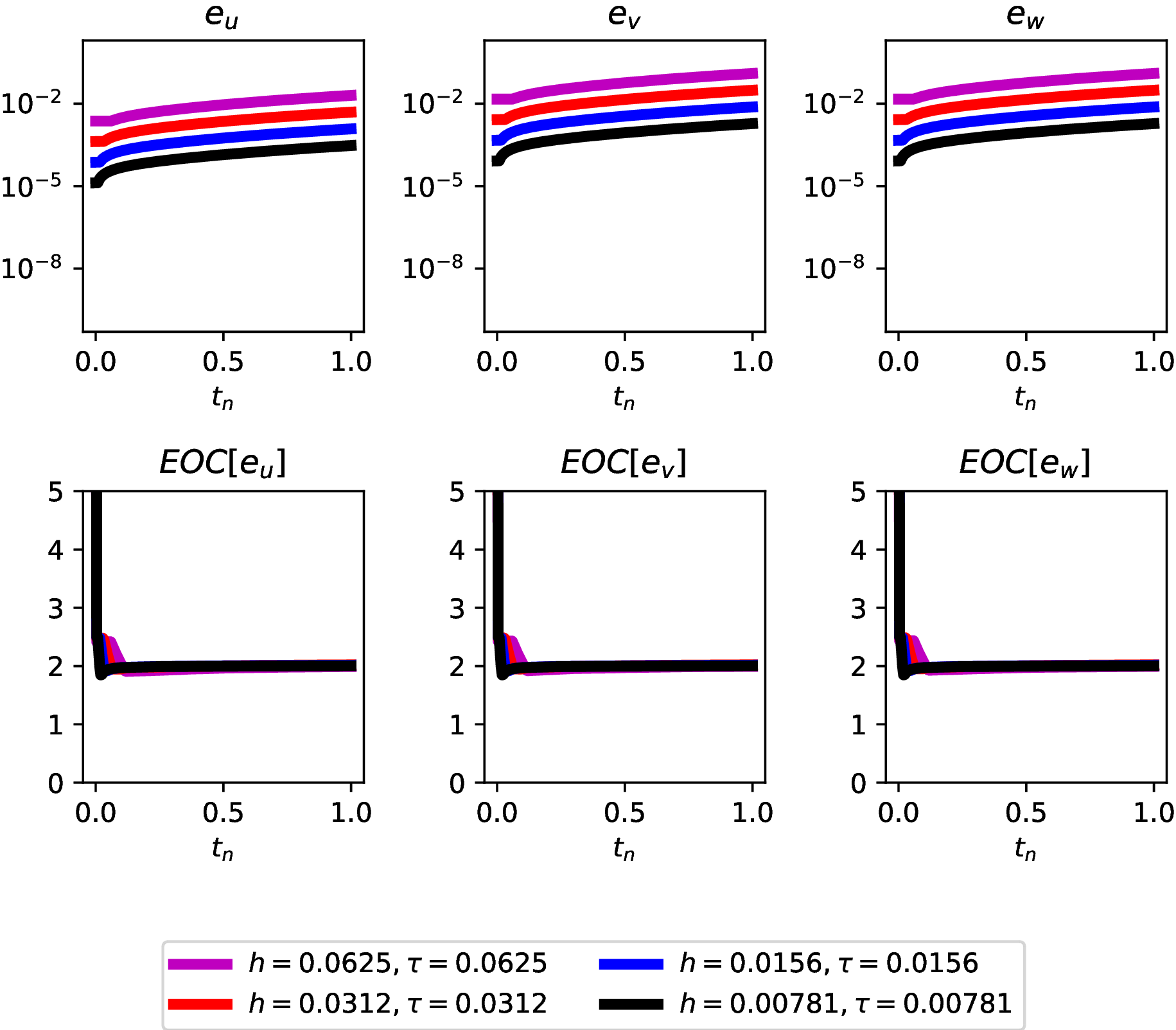
((a)) $q=0$ and $p=1$

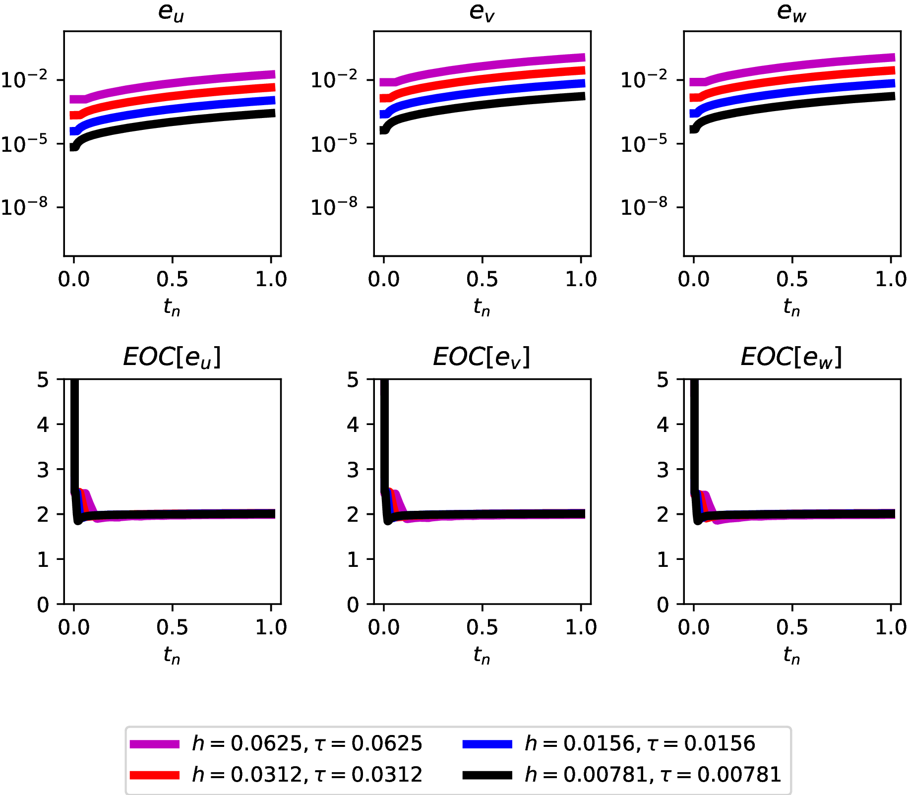
((b)) $q=0$ and $p=2$

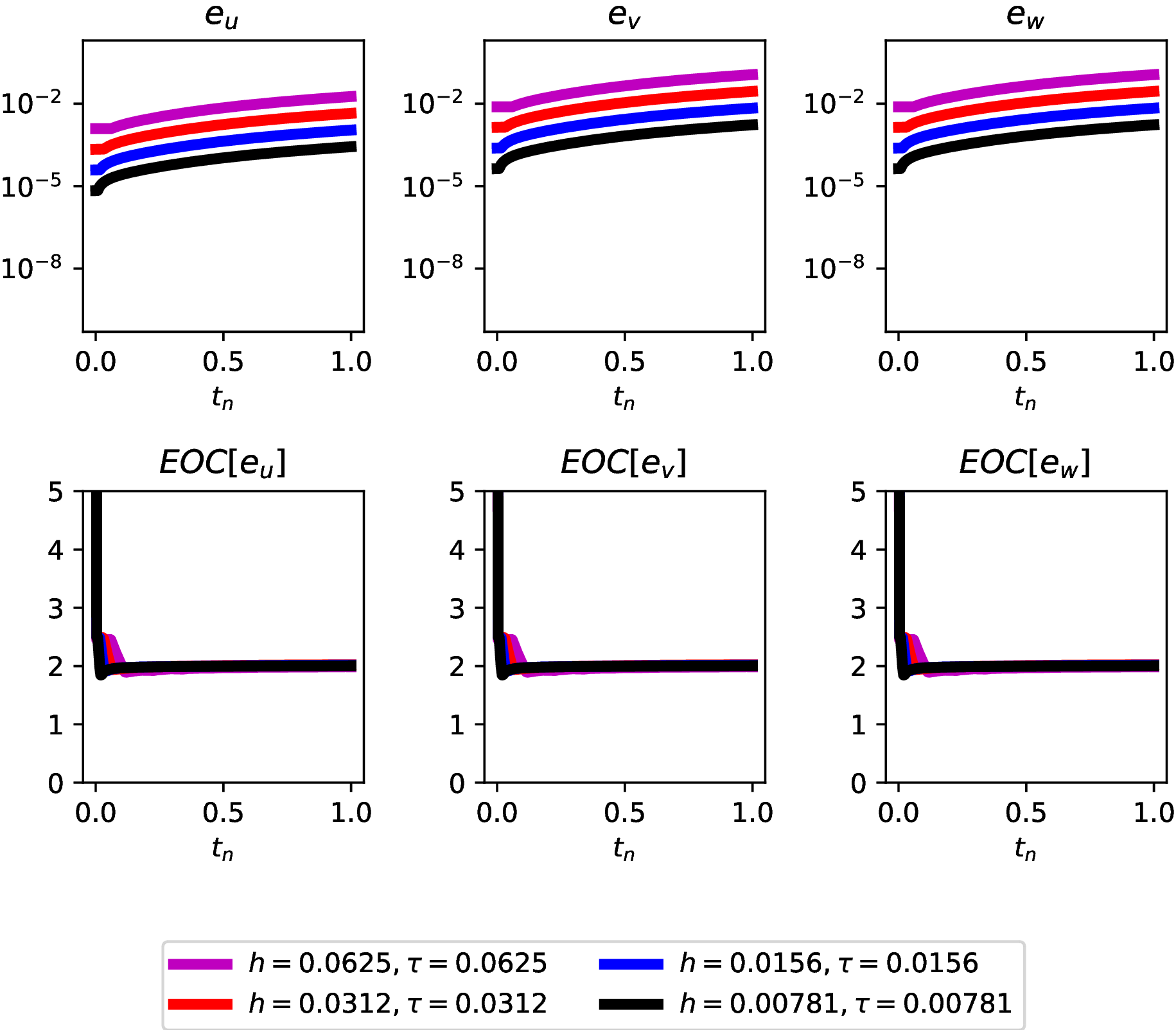
((c)) $q=0$ and $p=3$

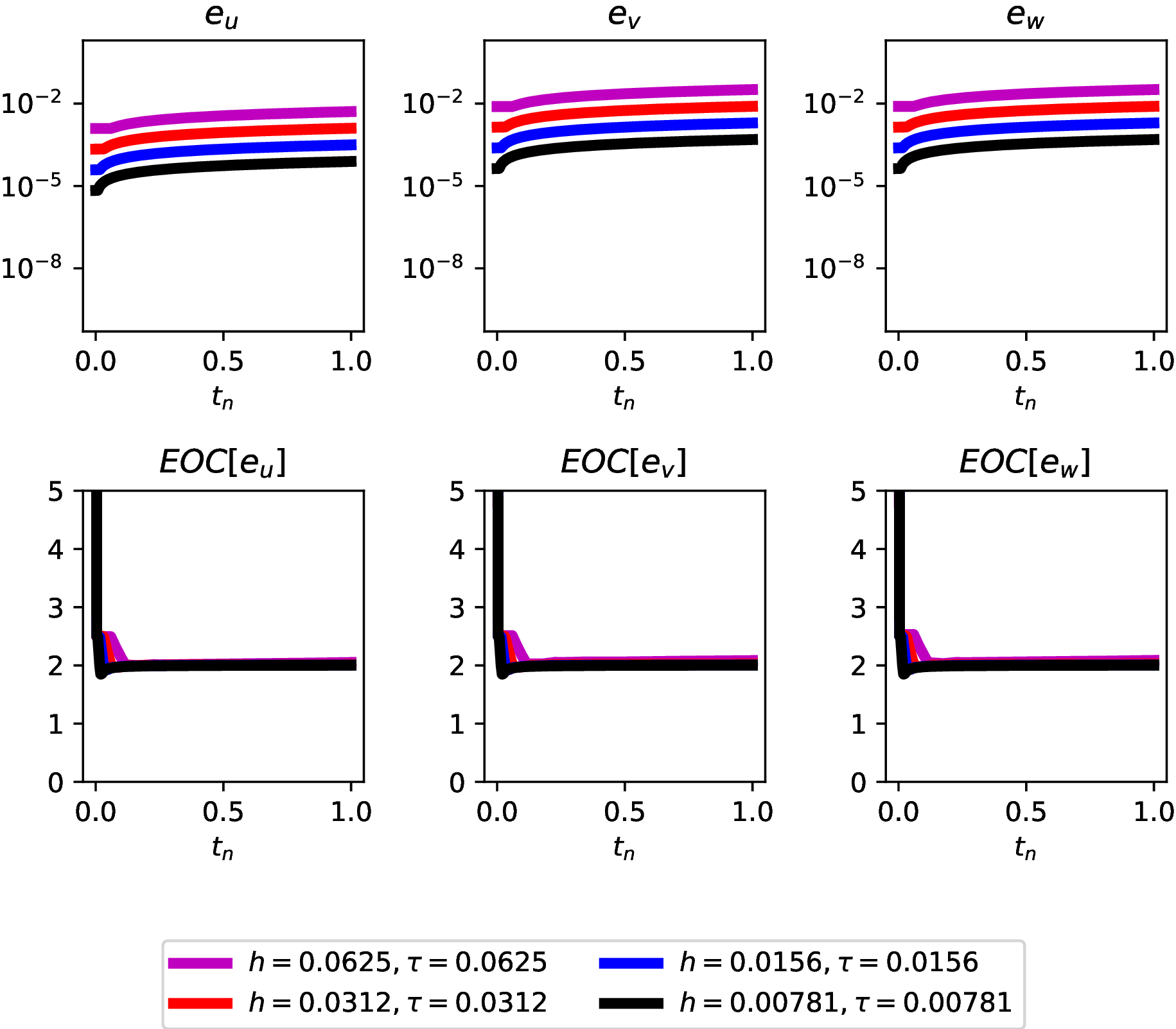
((d)) $q=1$ and $p=1$

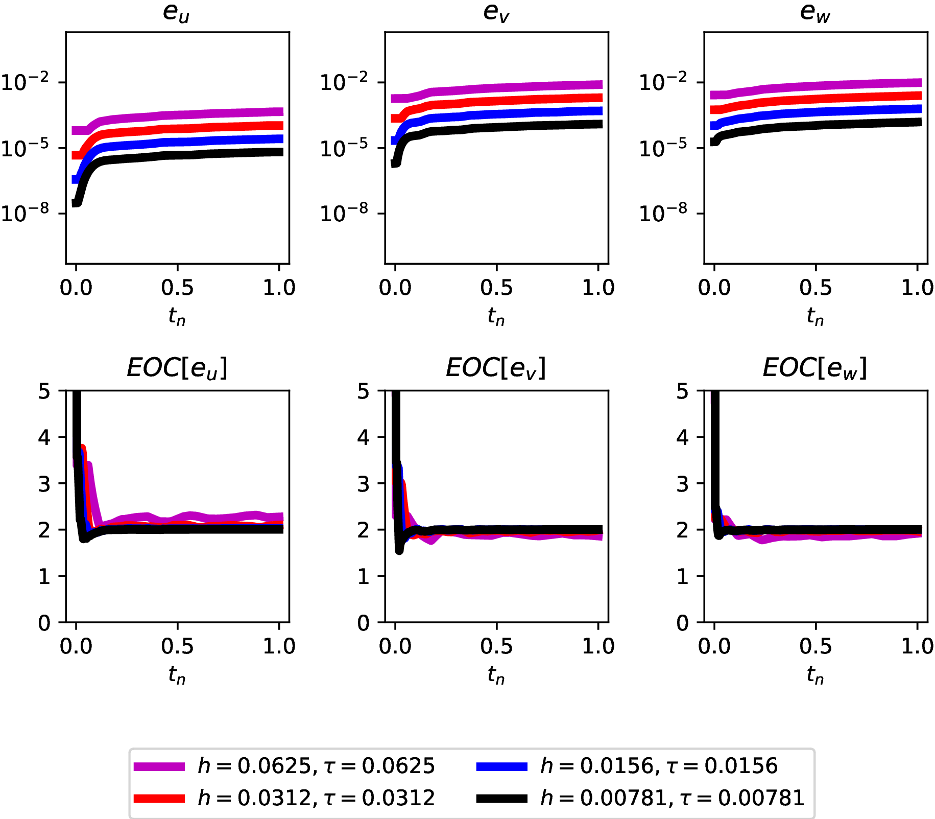
((e)) $q=1$ and $p=2$

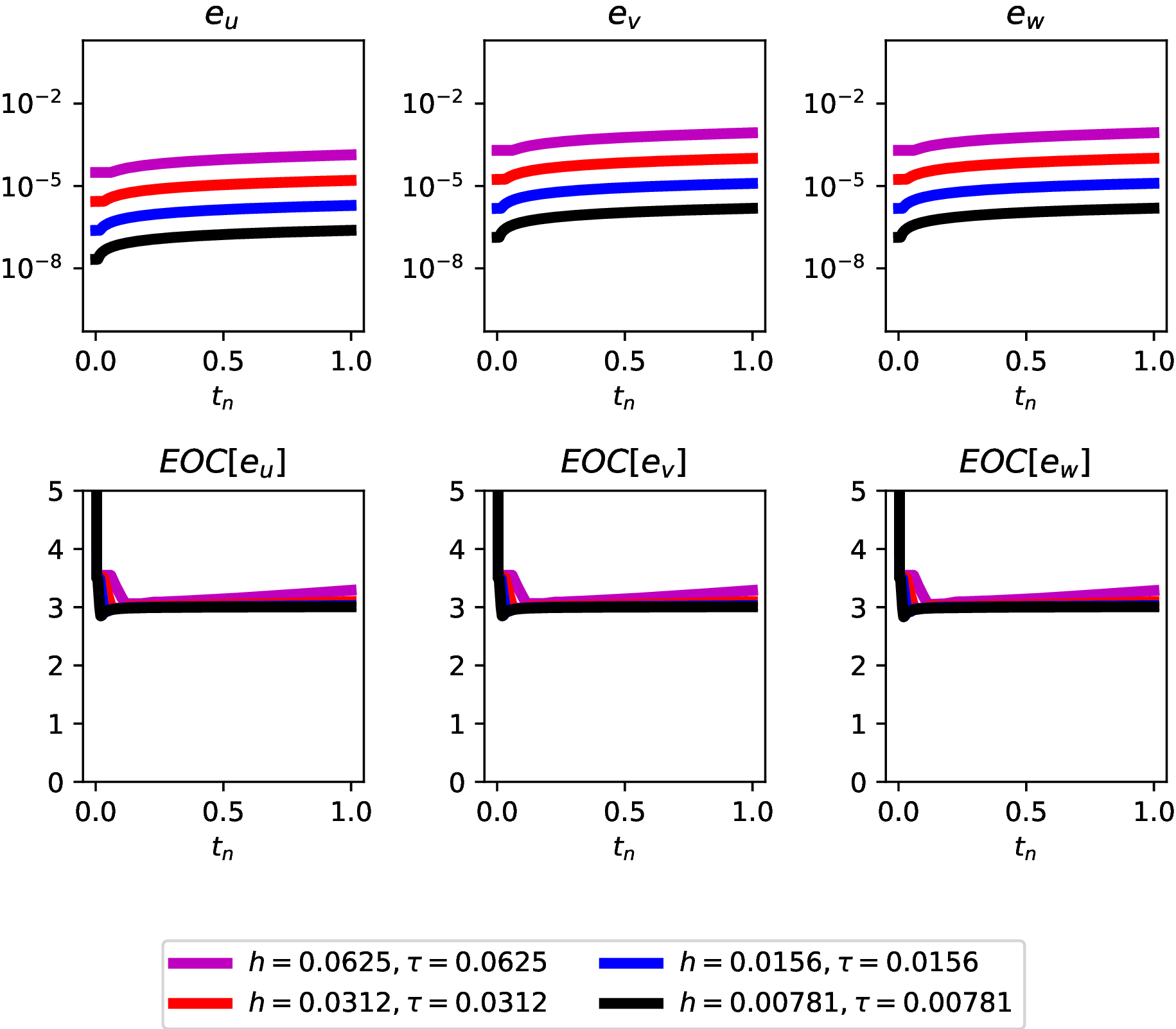
((f)) $q=1$ and $p=3$

((g)) $q=2$ and $p=1$

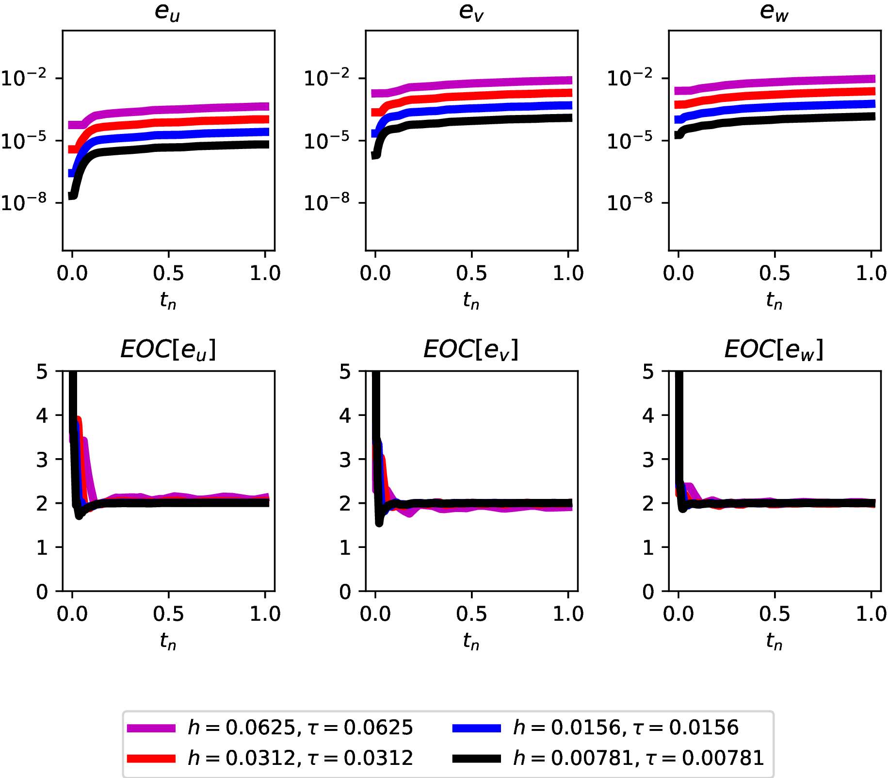
((h)) $q=2$ and $p=2$

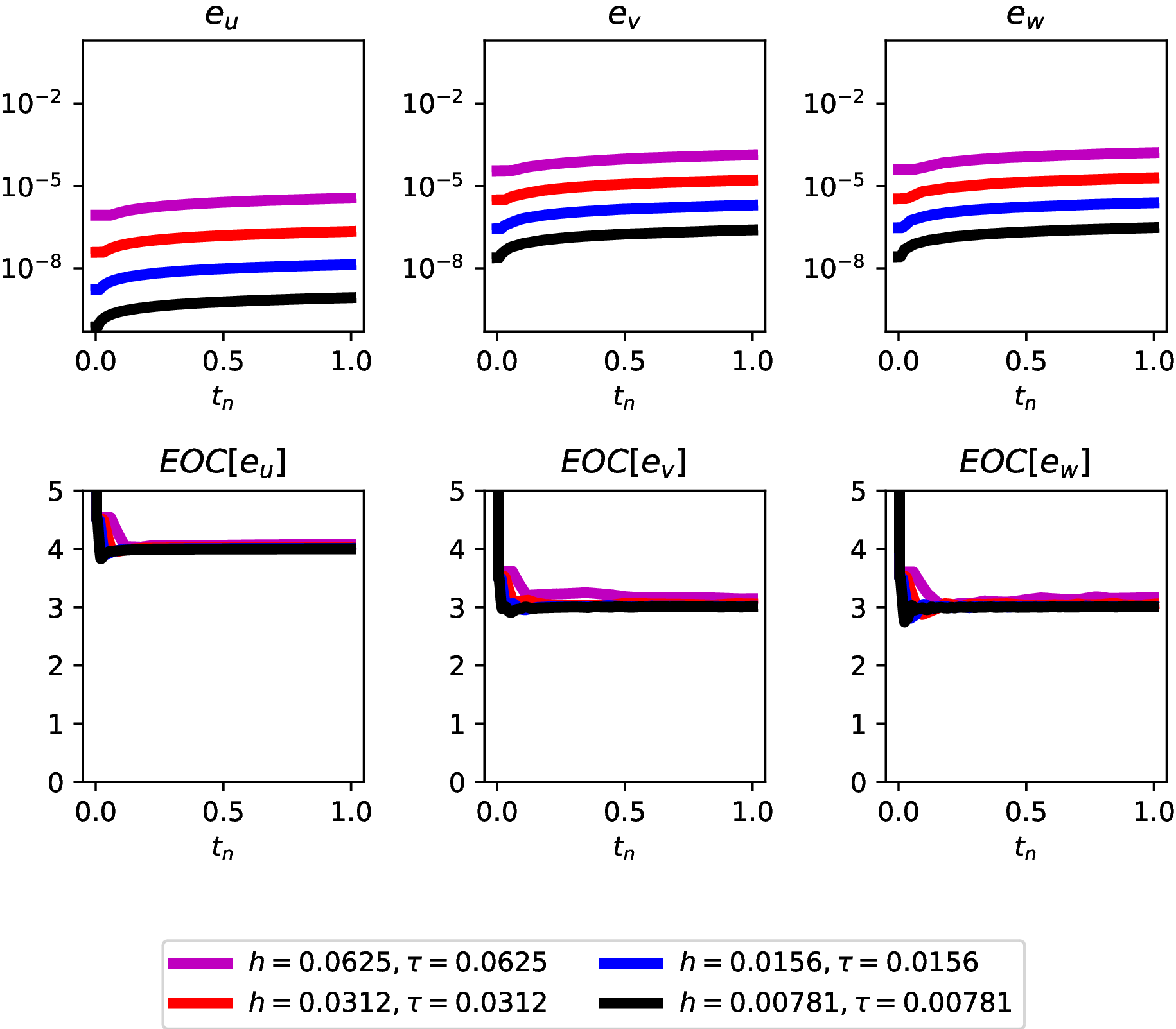
((i)) $q=2$ and $p=3$

Figure 5.1. The error of the spatially continuous finite element scheme (3.6) for the linear wave equation (5.7) initialised by the exact solution (5.8). Here $e_{u},e_{v},e_{w}$ denotes the errors in the components $U,V,W$ measured in the Bochner norm (5.2). Below we plot the EOC (5.1) corresponding to each of these errors.

Within this figure we consider the errors for the solution $U$ and the auxiliary variables independently. We shall now focus our attention to the error in $U$, denoted $e_{u}$. The simulations suggest a temporal experimental order of accuracy of $\mathcal{O}\left(\tau^{q+2}\right)$, which is optimal in time. However, spatially we observe that for $p$ even we obtain sub-optimal convergence at rate $\mathcal{O}\left(h^{q}\right)$, but for odd $p$ we converge optimally at rate $\mathcal{O}\left(h^{q+1}\right)$. This phenomenon is supported by more extensive numerical experimentation.

Instead simulating the spatially discontinuous finite element approximation (4.5) for the linear wave equation we obtain the errors and EOCs shown in Figure 5.2.

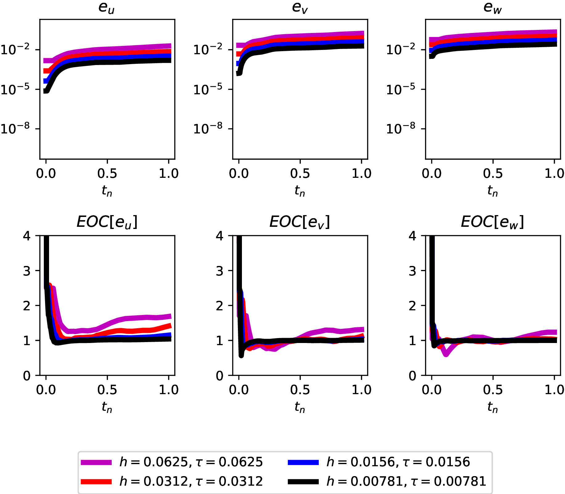
((a)) $q=0$ and $p=1$

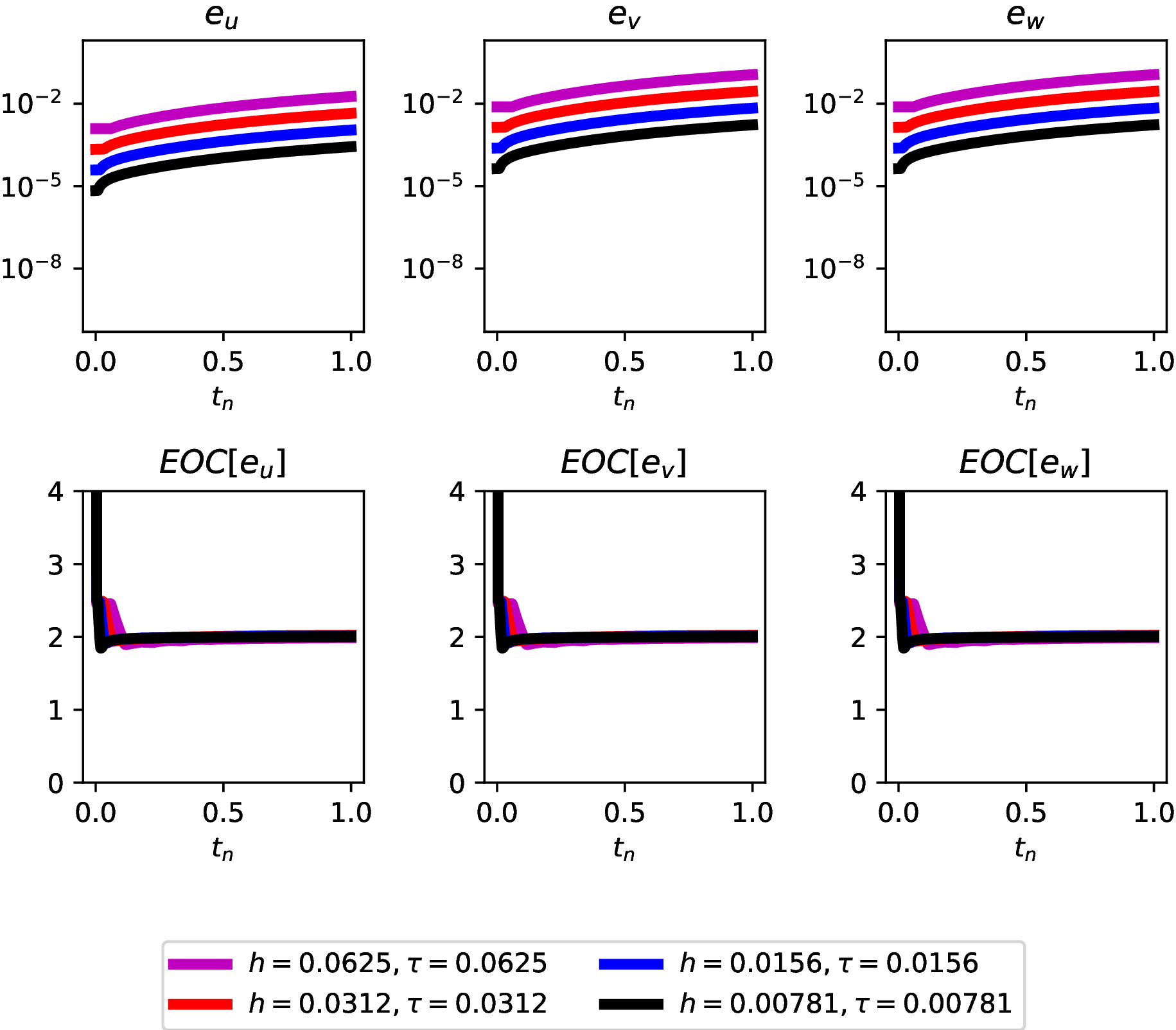
((b)) $q=0$ and $p=2$

((c)) $q=0$ and $p=3$

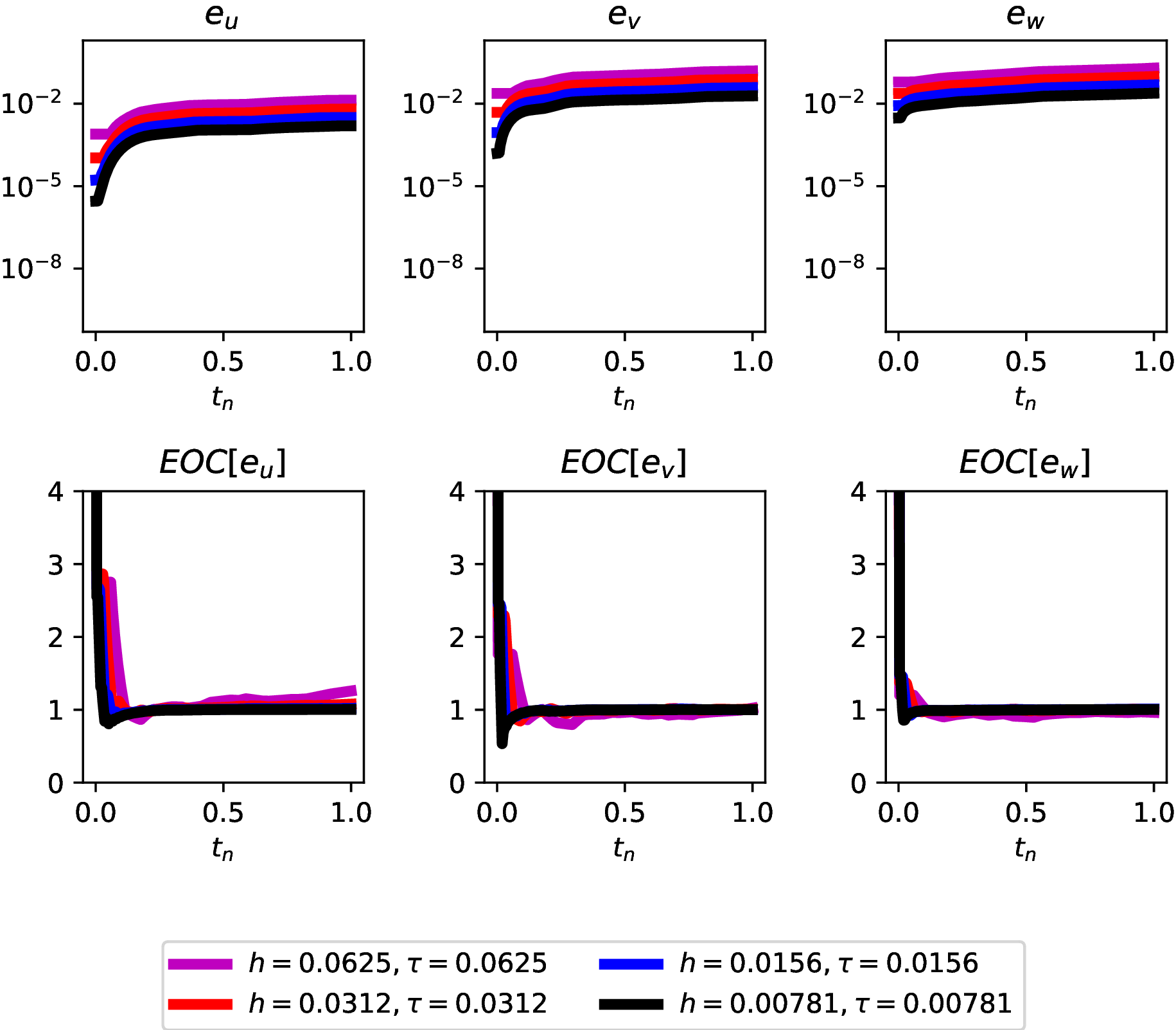
((d)) $q=1$ and $p=1$

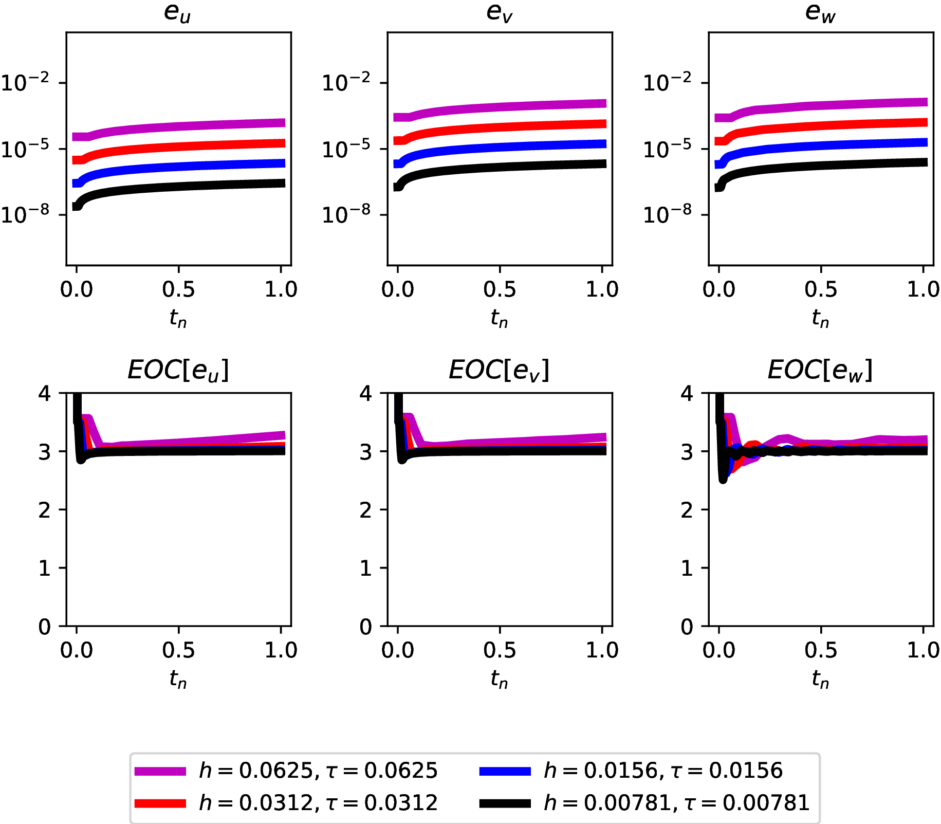
((e)) $q=1$ and $p=2$

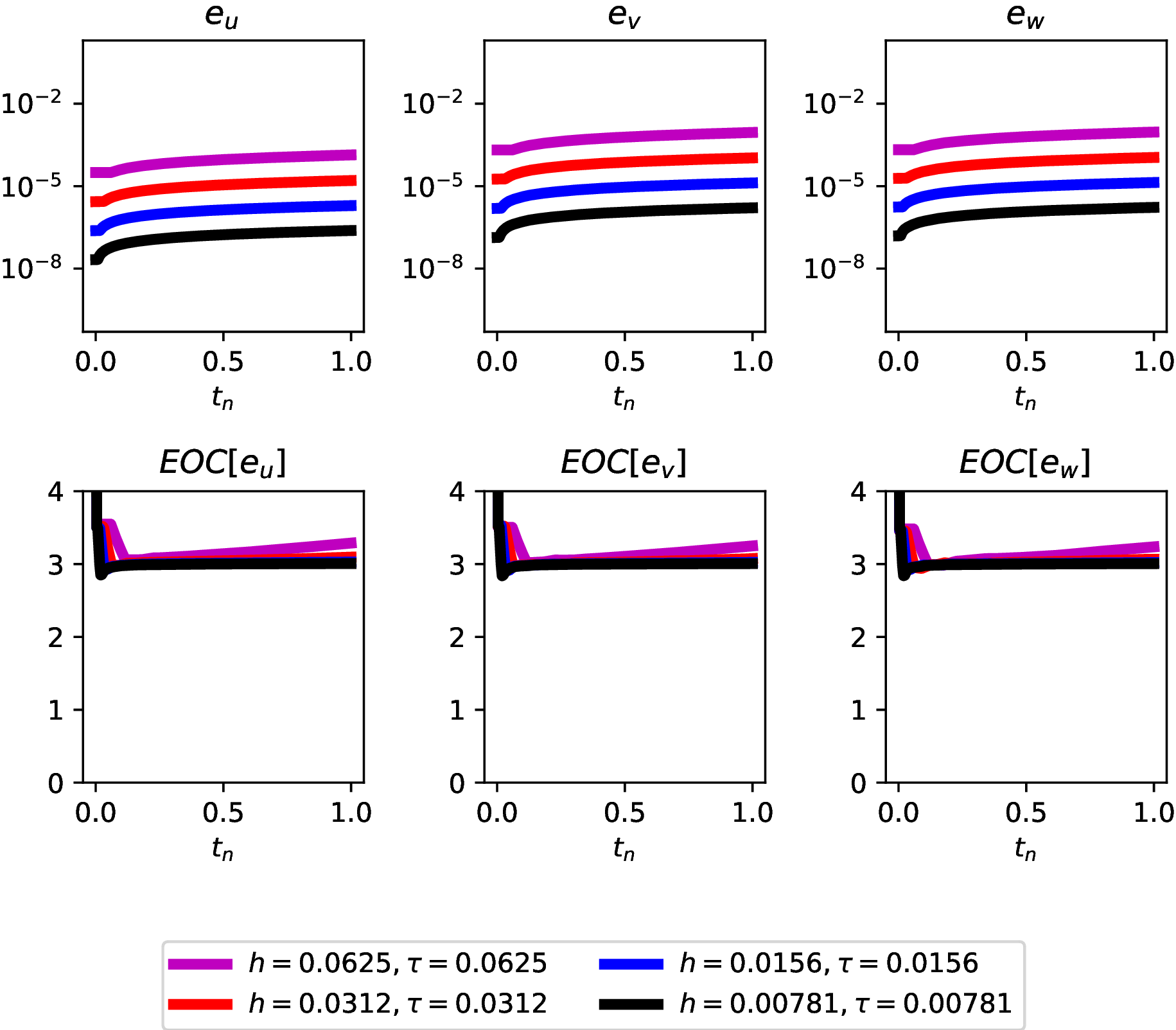
((f)) $q=1$ and $p=3$

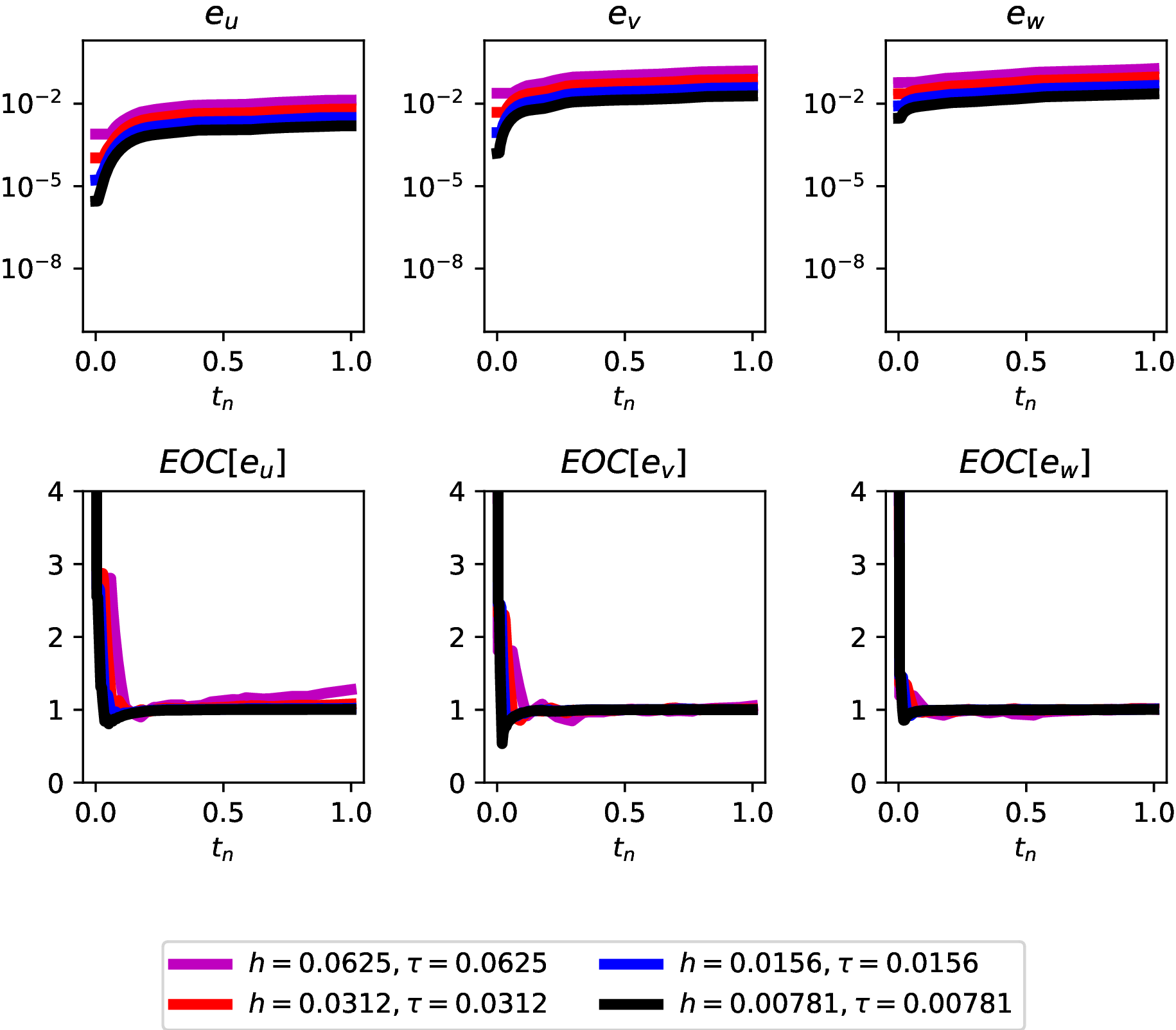
((g)) $q=2$ and $p=1$

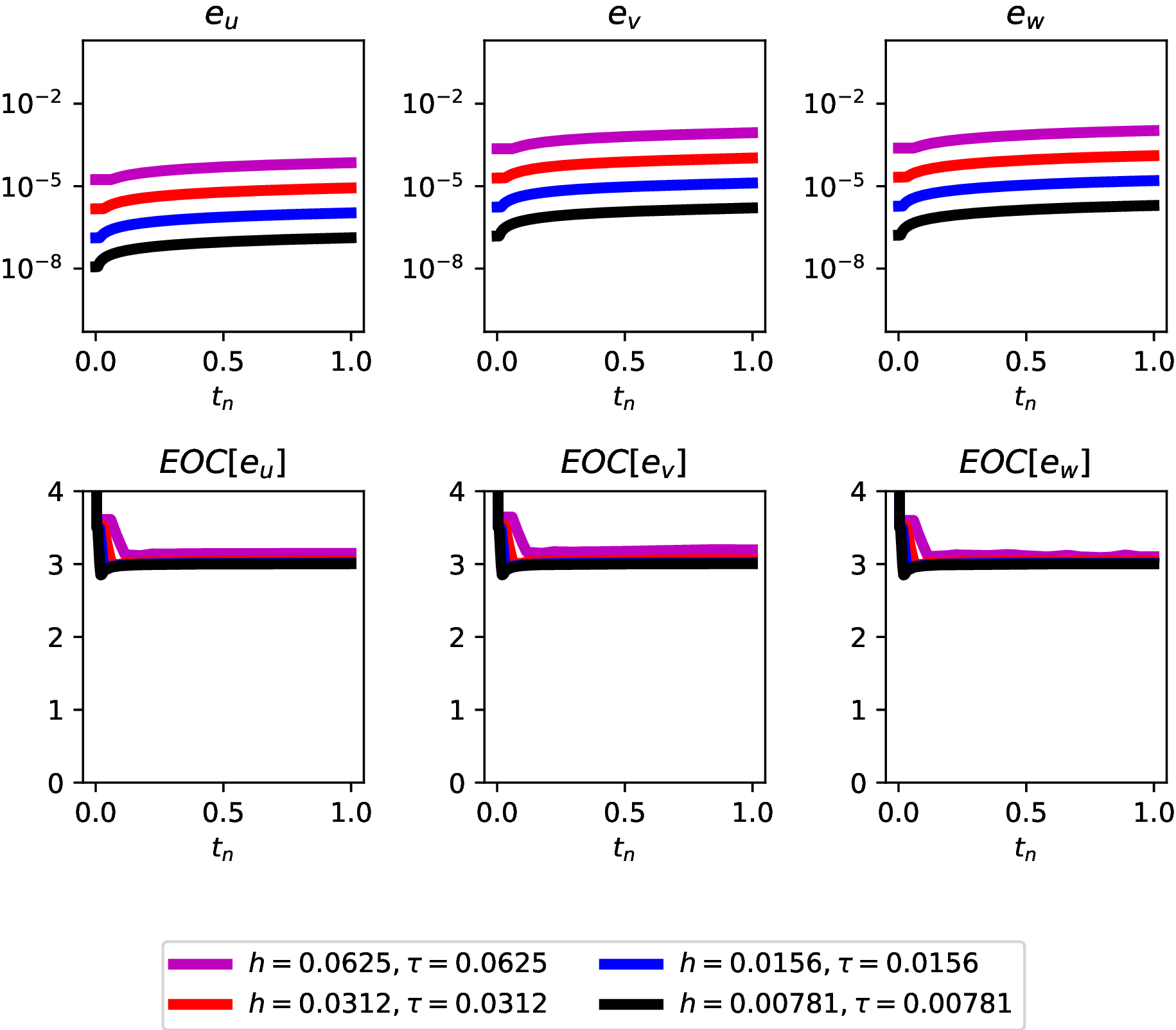
((h)) $q=2$ and $p=2$

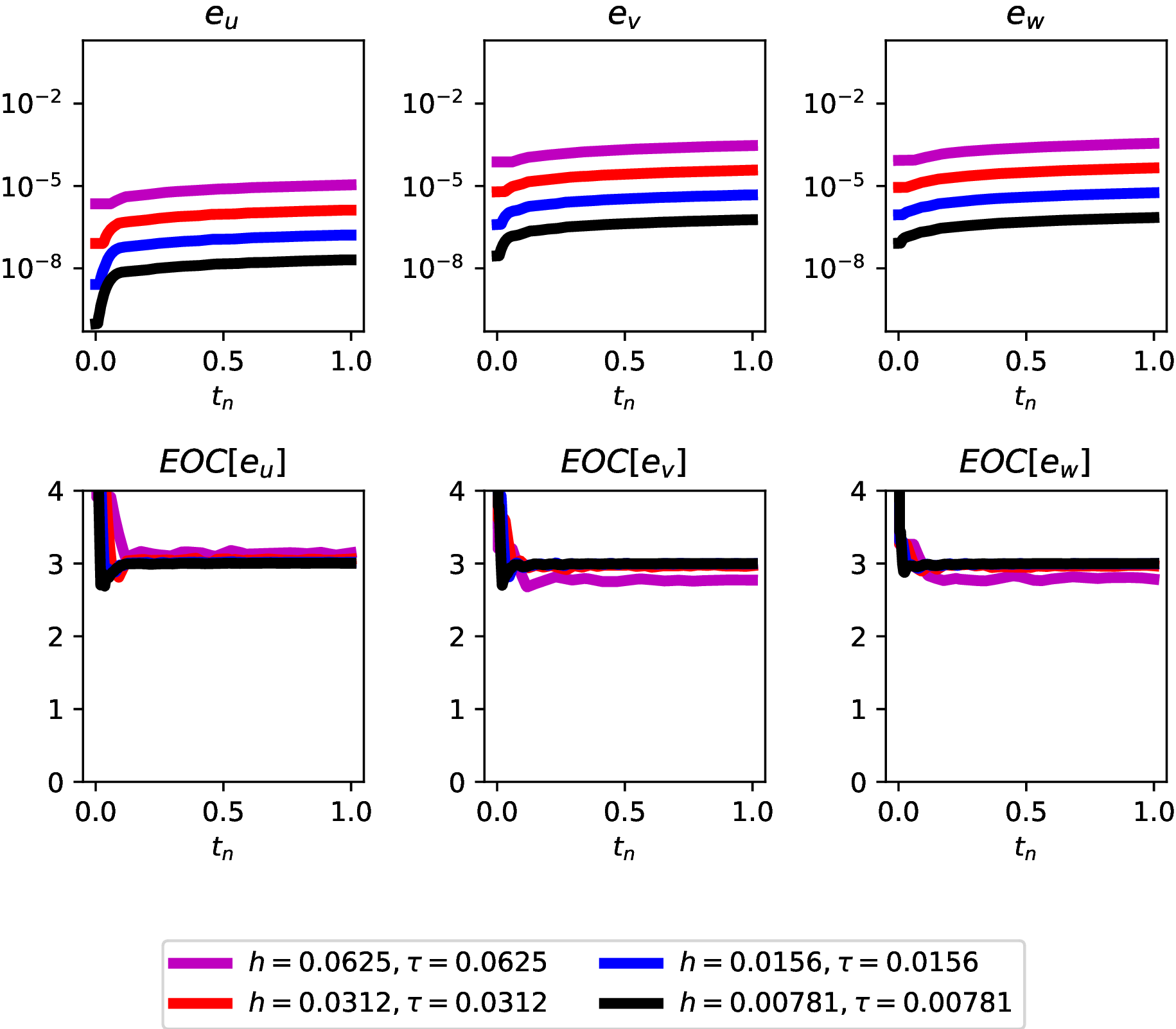
((i)) $q=2$ and $p=3$

Figure 5.2. The error of the spatially discontinuous finite element scheme (4.5) for the linear wave equation (5.7) initialised by the exact solution (5.8). Here $e_{u},e_{v},e_{w}$ denotes the errors in the components $U,V,W$ measured in the Bochner norm (5.2). Below we plot the EOC (5.1) corresponding to each of these errors.

These simulations suggest a temporal experimental order of accuracy of $\mathcal{O}\left(\tau^{q+2}\right)$, as expected as our temporal discretisation is identical to the previous simulation. However, spatially we observe that for $p$ odd we obtain sub-optimal convergence at rate $\mathcal{O}\left(h^{q}\right)$, but for even $p$ we converge optimally at rate $\mathcal{O}\left(h^{q+1}\right)$. This sub-optimality is also observed in the spatially continuous case however the sub-optimal and optimal cases are reversed. This phenomenon is supported by more extensive numerical experimentation. In this case it is likely caused by issues with the spatial first derivative operator $\mathcal{G}$, which is known to lack uniqueness for $p$ odd, see [34]. We may resolve this sub-optimal convergence for the linear wave equation by modifying $\mathcal{G}$ appropriately such that the spatial derivatives involve an appropriate mix of upwind and downwind fluxes as in [27], however the resulting discretisation not be valid for an arbitrarily multisymplectic PDE.

Further to these convergence simulations, all numerical simulations for the linear wave equation preserve the momentum (5.5) and energy (5.6) up to machine precision locally.

5.2. Test 2: The nonlinear wave equation

Throughout this test we shall restrict ourselves to the spatially continuous scheme, as the numerical results do not differ in the spatially discontinuous case. Instead choosing the potential in Example 2.6 to be $\mathcal{V}(u)=\frac{1}{4}u^{4}$ we obtain a nonlinear wave equation. We may explicitly rewrite the multisymplectic formulation as the system

$$\begin{split}v_{t}-w_{x}+\mathcal{V}^{\prime}(u)&=0\\ v-u_{t}&=0\\ w-u_{x}&=0.\end{split}$$ (5.9)

In this setting, our proposed finite element scheme (3.5) and the momentum conserving alternative (3.25) are distinct. In addition to the conservation laws obtained via the multisymplectic structure we also expect simulations to be mass conserving, i.e.,

$$\int_{S^{1}}U\left(t_{n},x\right)\text{ }\mathrm{d}{x}=\int_{S^{1}}U\left(0,x\right)\text{ }\mathrm{d}{x}.$$ (5.10)

Through fixing $\tau=0.1$ and $h=0.01$ we run extensive numerical simulations investigating the deviation in mass, momentum (5.5) and energy (5.6) in Figure 5.3.

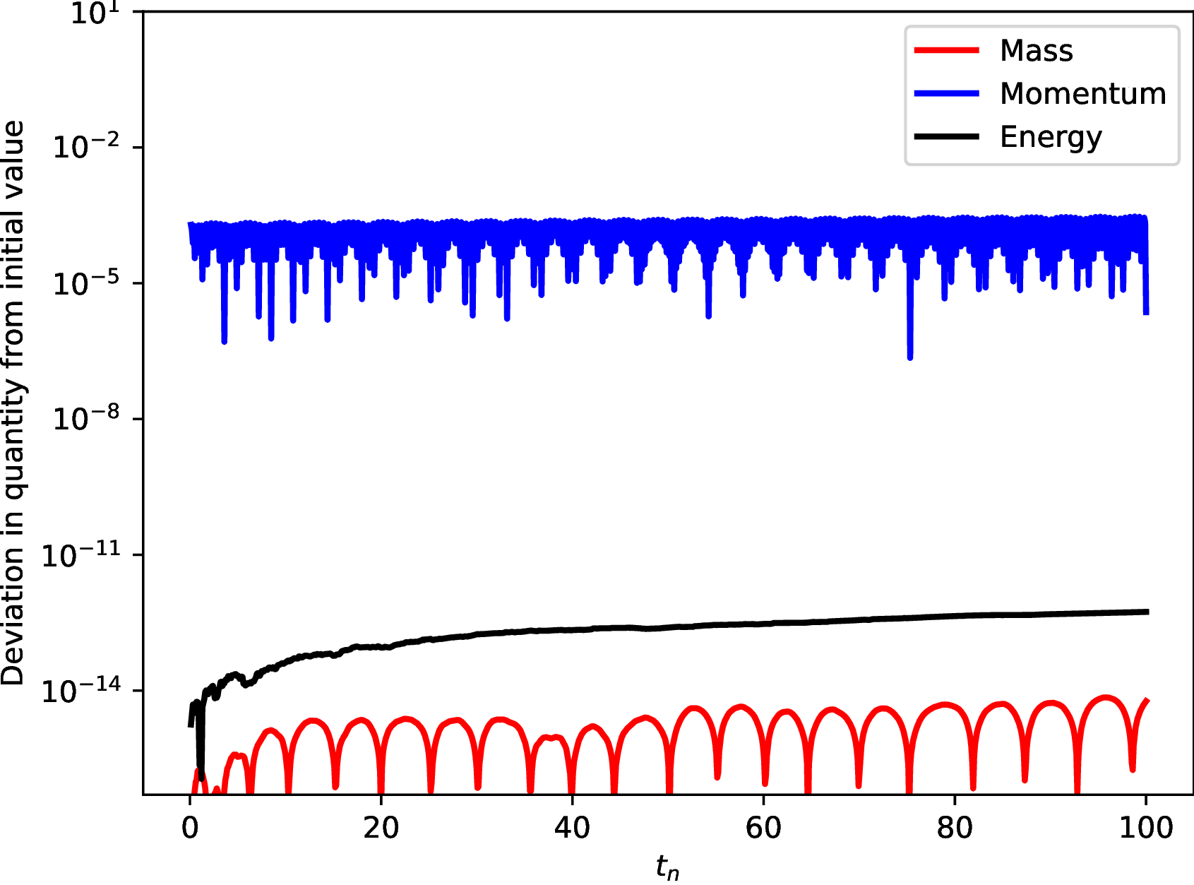
((a)) $q=0$ and $p=1$

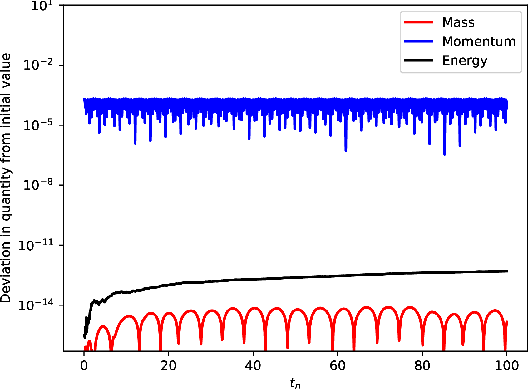
((b)) $q=0$ and $p=2$

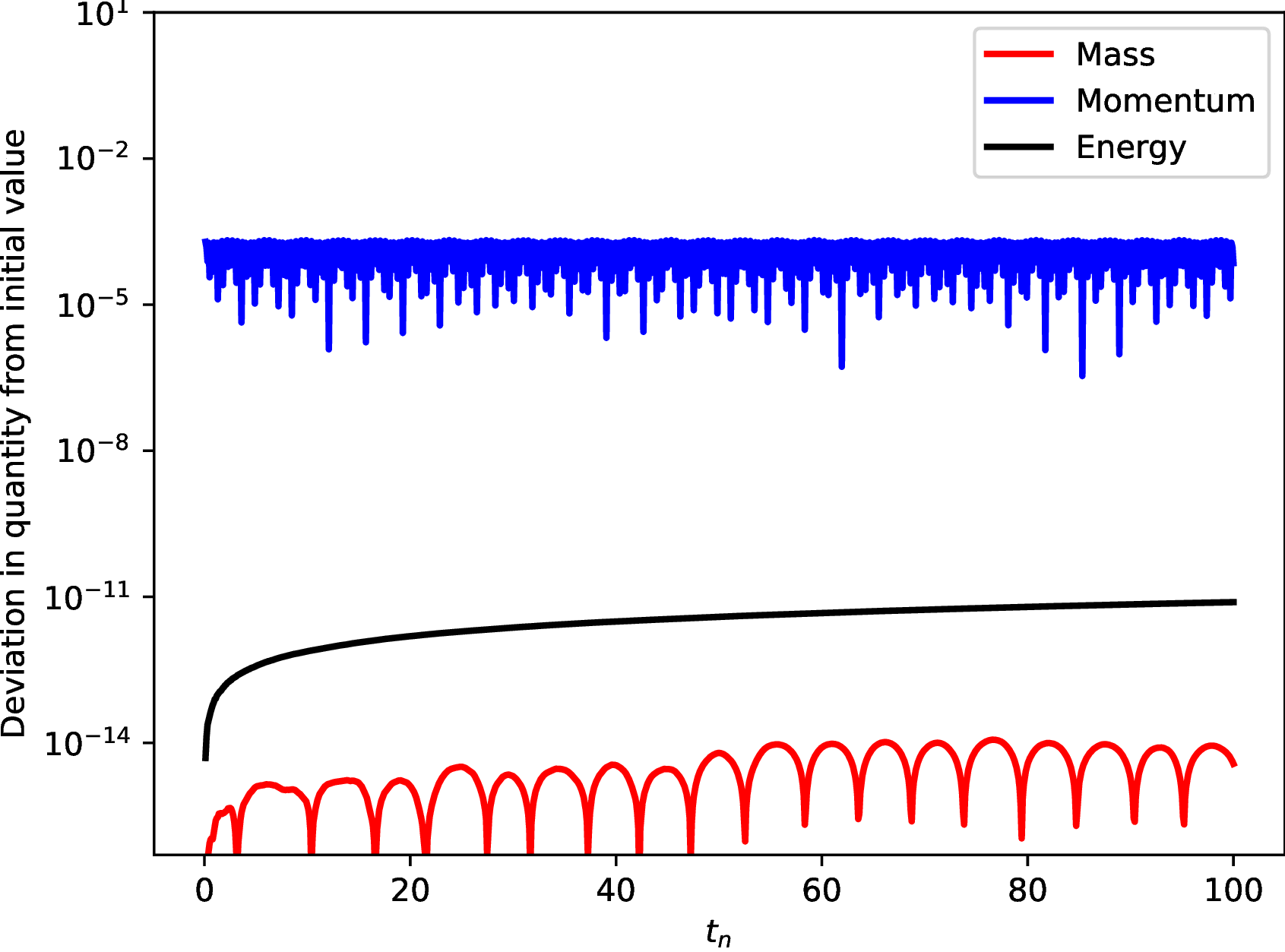
((c)) $q=0$ and $p=3$

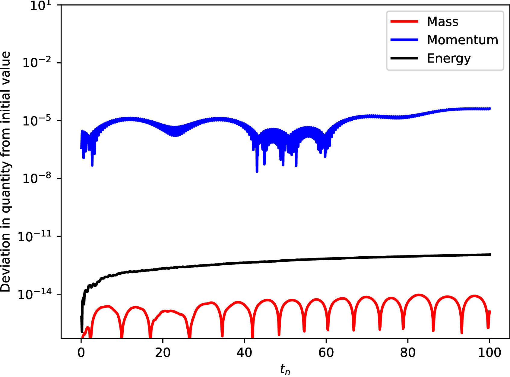
((d)) $q=1$ and $p=1$

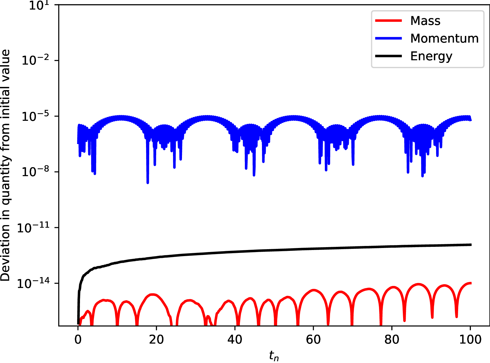
((e)) $q=1$ and $p=2$

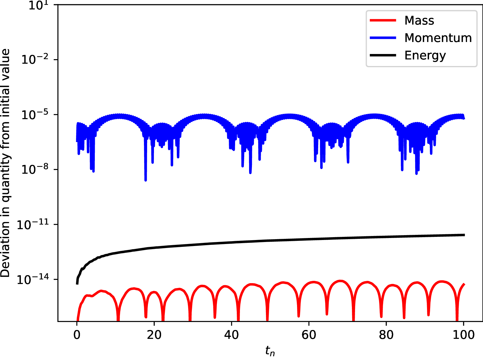
((f)) $q=1$ and $p=3$

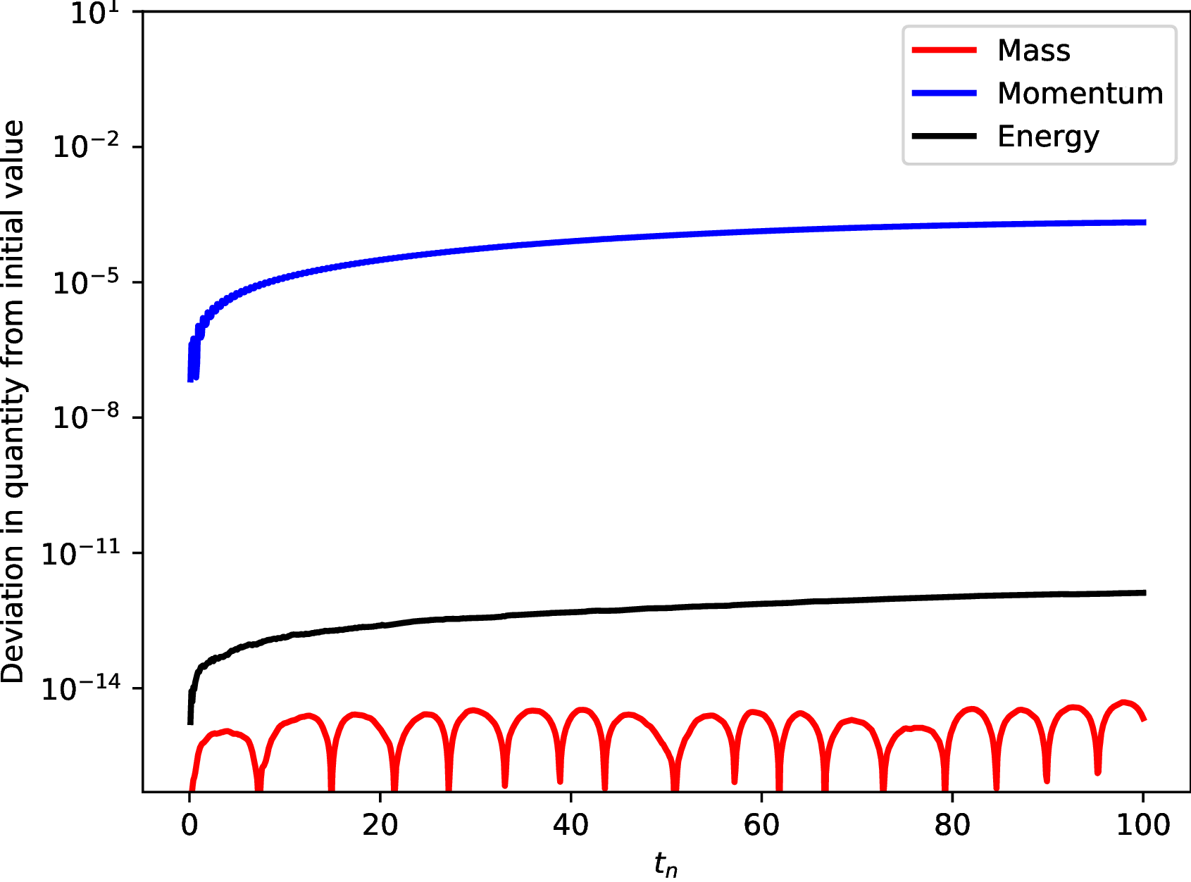
((g)) $q=2$ and $p=1$

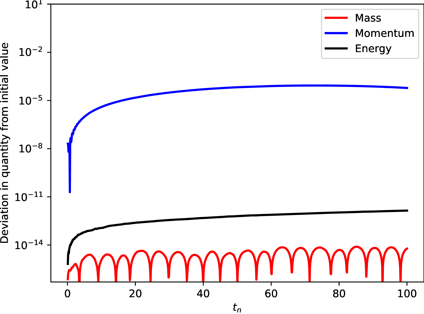
((h)) $q=2$ and $p=2$

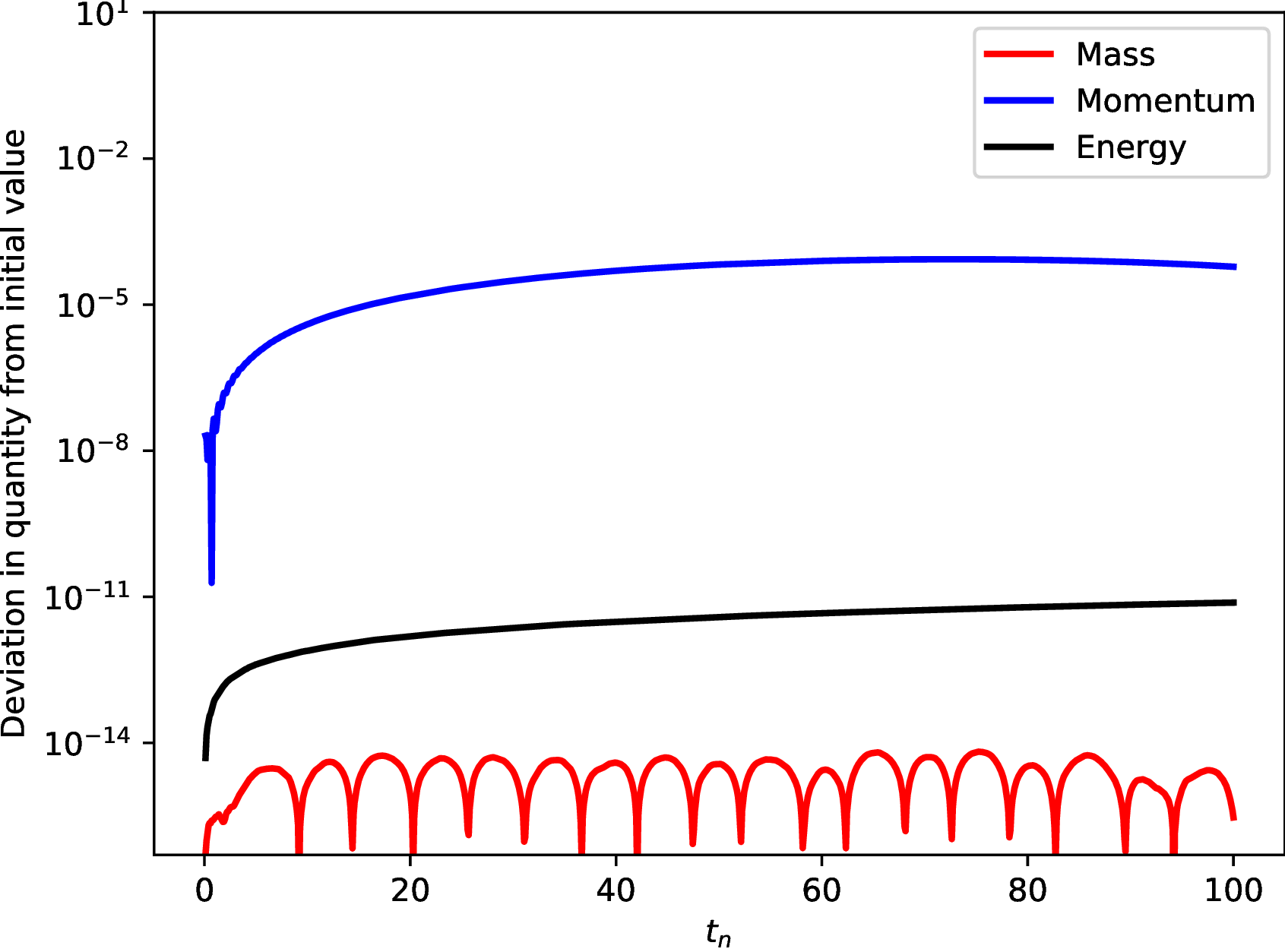
((i)) $q=2$ and $p=3$

Figure 5.3. The deviation in the conservation laws (5.10), (5.5) and (5.6) for the spatially continuous finite element scheme (3.6) for the nonlinear wave equation (5.9) initialised by the exact solution (5.8) with varying temporal degree $q$ and spatial degree $p$. All simulations have uniform temporal and spatial elements with $\tau=0.1$ and $h=0.01$. We notice that the energy density is exactly preserved locally over time and globally over space. The deviation in momentum, while not exactly preserved, remains bounded over long time.

We observe that the energy density is indeed conserved locally in time and globally in space. Over long time errors below solver tolerance propagate in the energy, with this propagation becoming more significant for higher polynomial degree. For all simulations the deviation in mass does not propagate over long time, and the momentum remains bounded deviating by approximately $10^{-5}$.

Through a small perturbation to the finite element approximation, namely that made within Remark 3.10 with (3.10), we also investigate the numerical deviation in conservation laws in Figure 5.4.

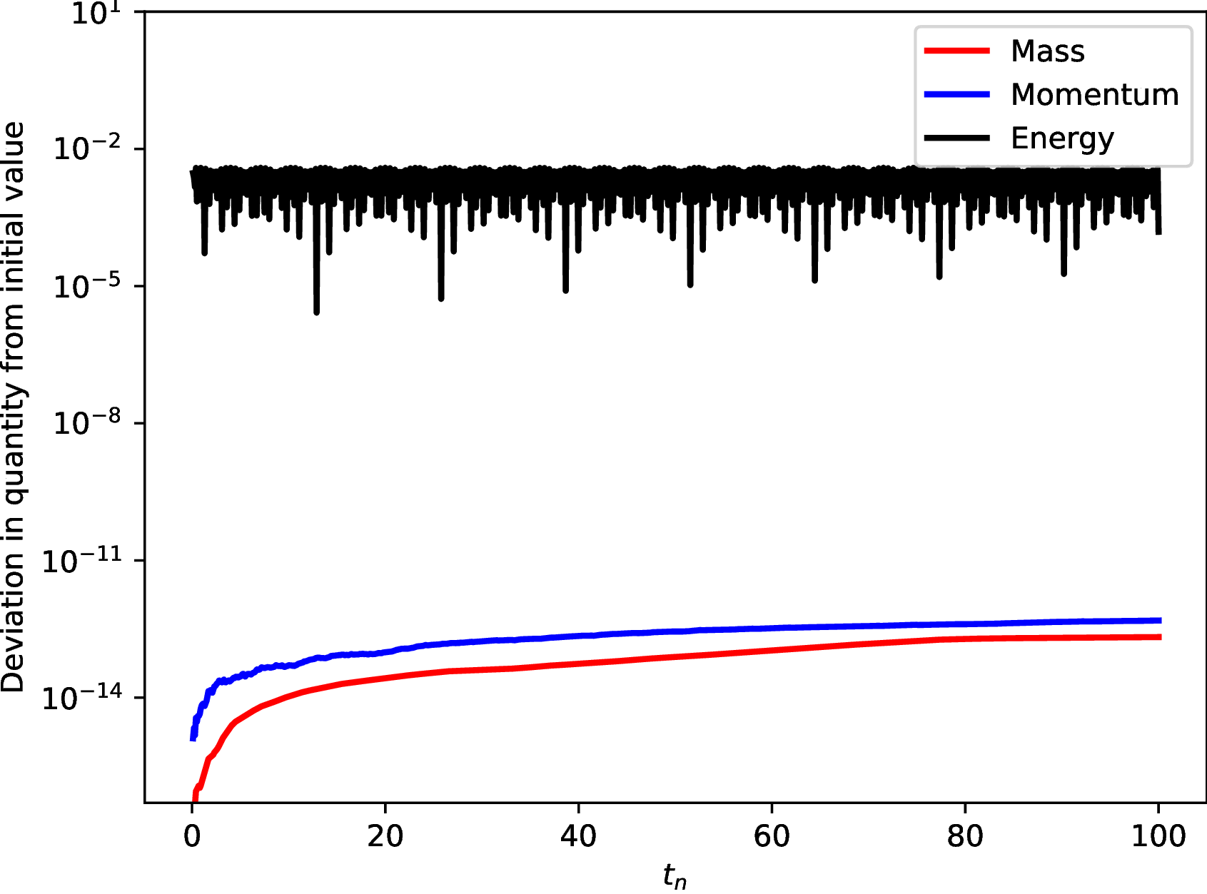
((a)) $q=0$ and $p=1$

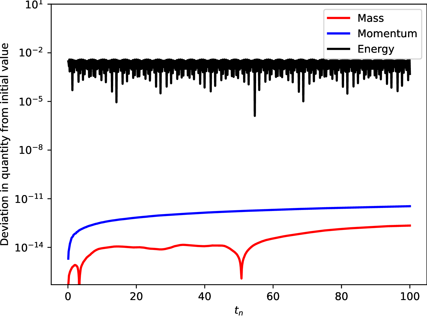
((b)) $q=0$ and $p=2$

((c)) $q=0$ and $p=3$

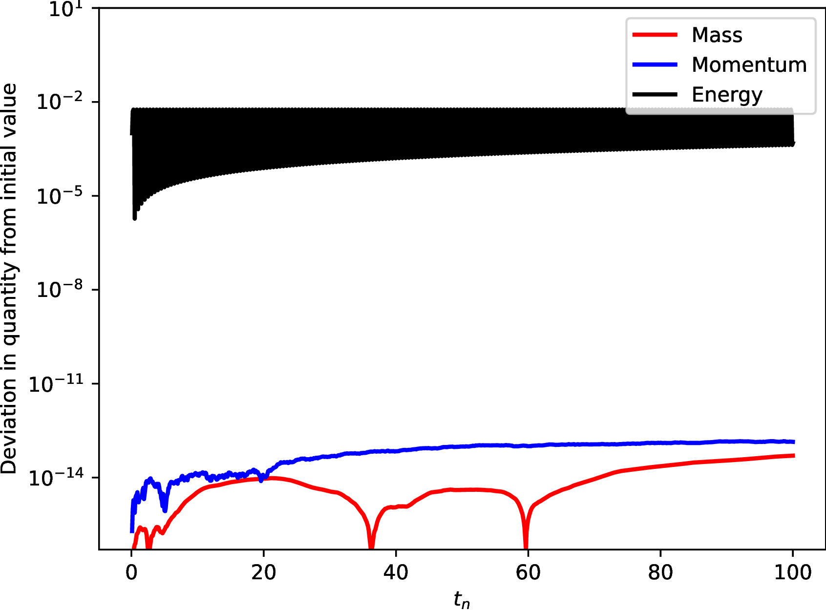
((d)) $q=1$ and $p=1$

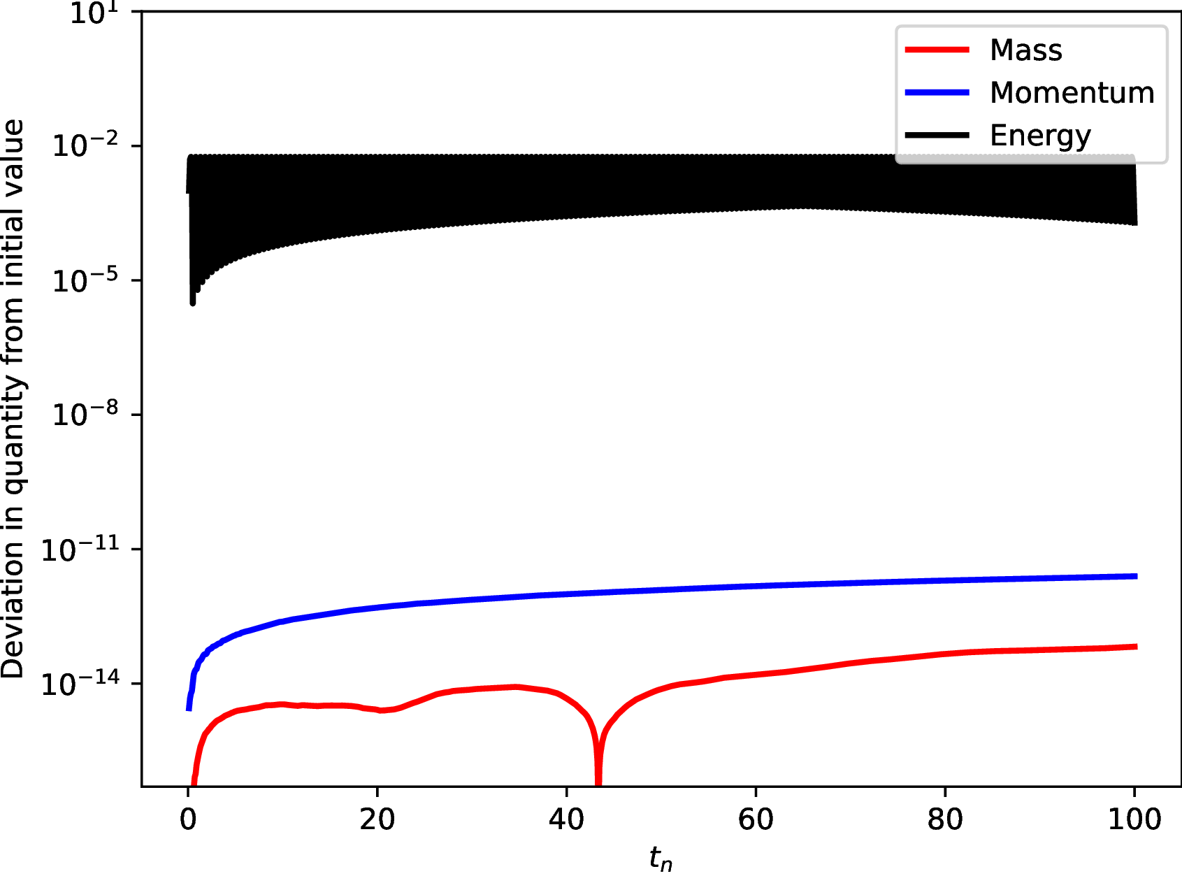
((e)) $q=1$ and $p=2$

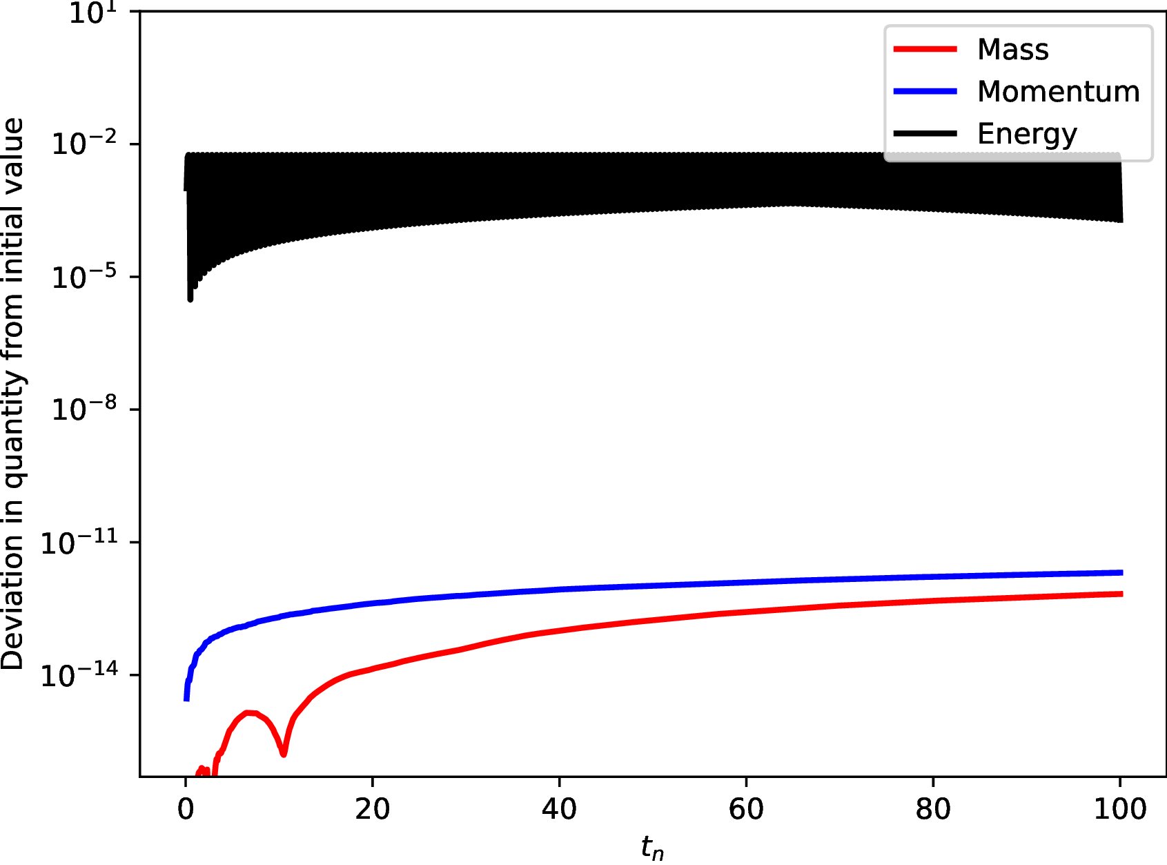
((f)) $q=1$ and $p=3$

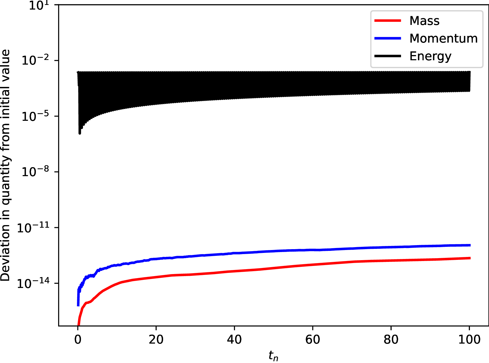
((g)) $q=2$ and $p=1$

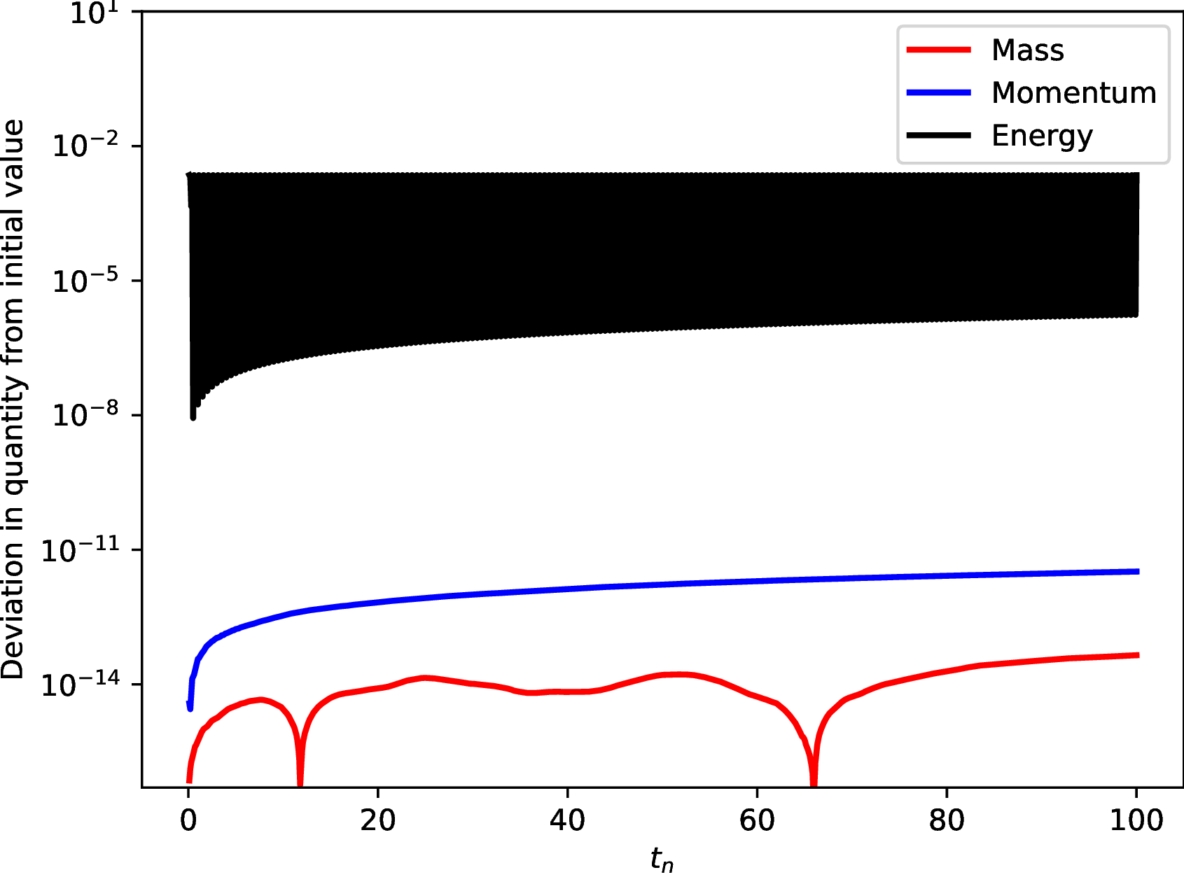
((h)) $q=2$ and $p=2$

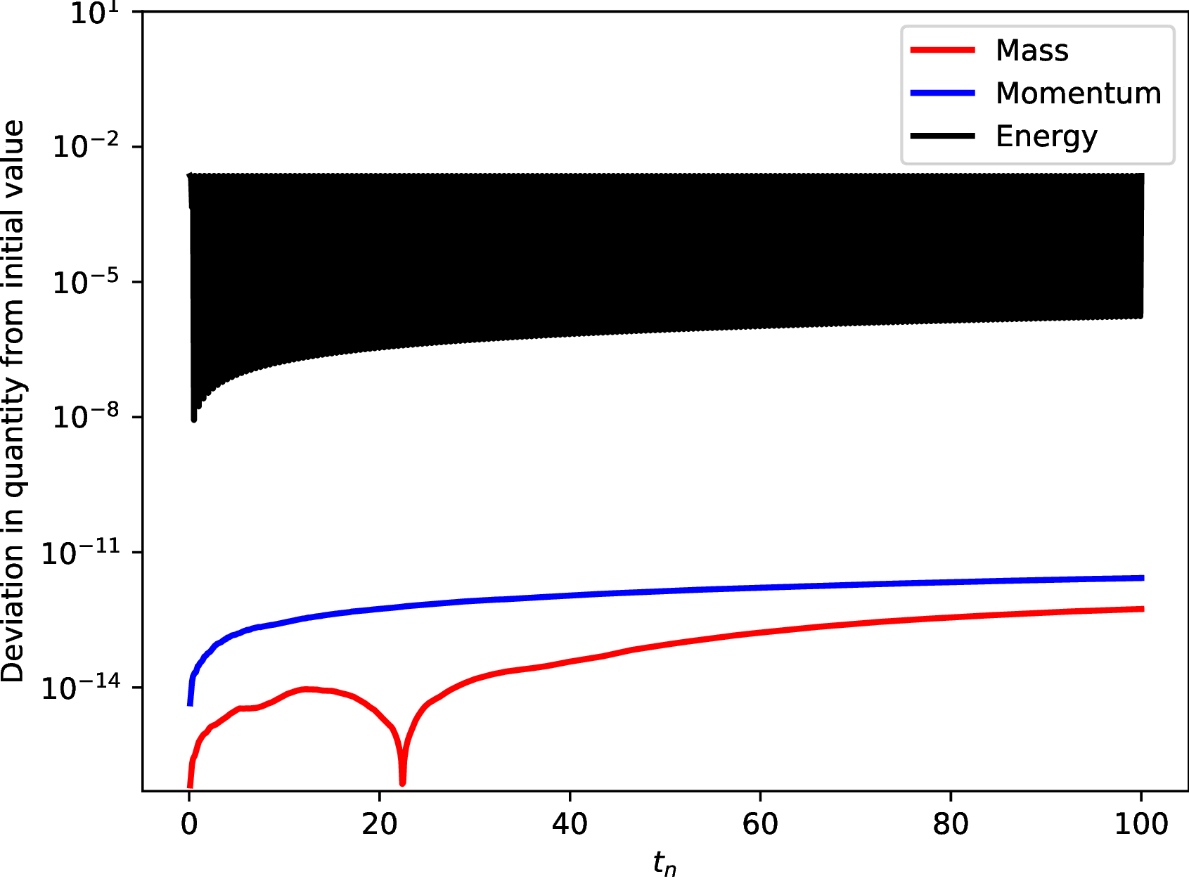
((i)) $q=2$ and $p=3$

Figure 5.4. The deviation in the conservation laws (5.10), (5.5) and (5.6) for the alternative finite element scheme (3.6) for the nonlinear wave equation (5.9) initialised by the exact solution (5.8) with varying temporal degree $q$ and spatial degree $p$. All simulations have uniform temporal and spatial elements with $\tau=0.1$ and $h=0.01$. We notice that the momentum density is exactly preserved locally over time and globally over space. The deviation in energy, while not exactly preserved, remains bounded over long time. Comparing against Figure 5.3 we notice the deviation in energy here is larger than the deviation in momentum for our primary discretisation (3.5), and does not globally decrease as we increase polynomial degrees.

We observe that while the modified scheme (3.25) does preserve the mass and momentum density locally over time and globally over space, the deviation of both propagates over long time leading to significant errors. In addition, the deviation in energy remains globally by $10^{-2}$ regardless of the polynomial degree of the approximation.

5.3. Test 3: The nonlinear Schrödinger equation

We may explicitly express the multisymplectic formulation of the NLS equation, given in Example 2.7, as

$$\begin{split}-v_{t}+p_{x}+\frac{1}{2}u\left(u^{2}+v^{2}\right)&=0\\ u_{t}+q_{x}+\frac{1}{2}v\left(u^{2}+v^{2}\right)&=0\\ -u_{x}+p&=0\\ -v_{x}+q&=0,\end{split}$$ (5.11)

see for example [31]. Throughout our numerical study, we initialise simulations of (5.11) with the soliton solution

$$\begin{split}u(t,x)&=2\mathrm{cos}\left(t\right)\mathrm{sech}\left(x\right)\\ v(t,x)&=2\mathrm{sin}\left(t\right)\mathrm{sech}\left(x\right)\\ p(t,x)&=-2\mathrm{cos}\left(t\right)\mathrm{sinh}\left(x\right)\mathrm{sech}\left(x\right)^{2}\\ q(t,x)&=-2\mathrm{sin}\left(t\right)\mathrm{sinh}\left(x\right)\mathrm{sech}\left(x\right)^{2},\end{split}$$ (5.12)

over the stretched periodic spatial domain of $x\in[0,40)$. We note that (5.12) is defined over $\mathbb{R}$, however, we may accurately approximate it on a periodic domain as it is a travelling wave.

Similarly to the linear wave equation, we may benchmark spatially continuous scheme for the nonlinear Schrödinger equation for various polynomial degree, as can be seen in Figure 5.5.

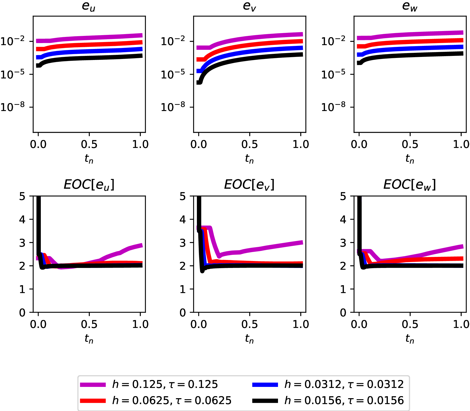
((a)) $q=0$ and $p=1$

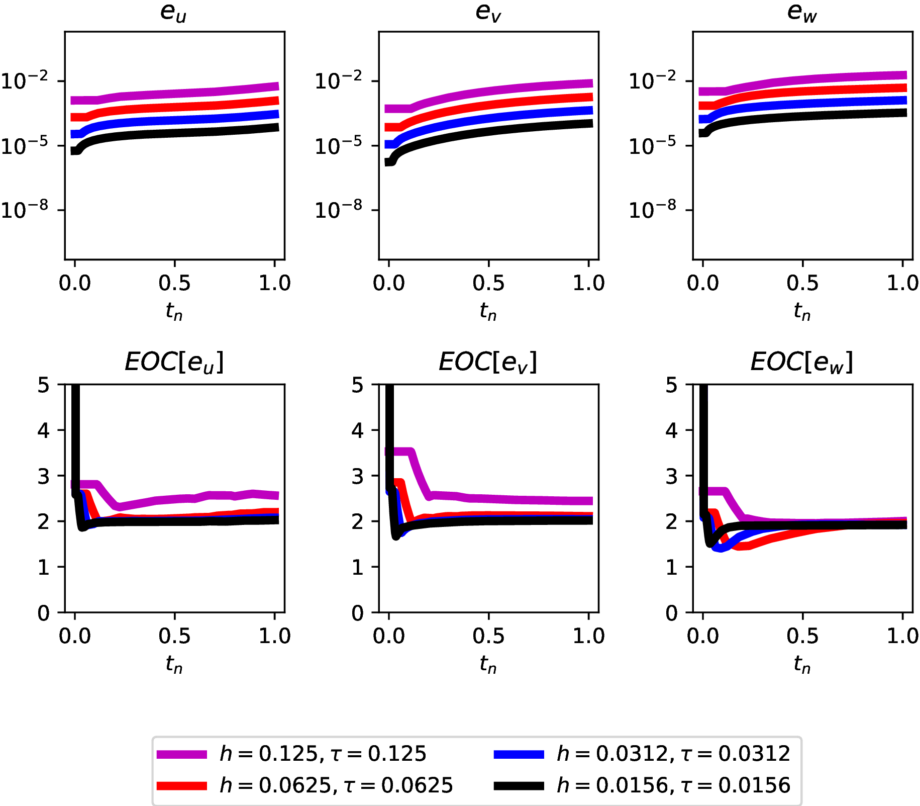
((b)) $q=0$ and $p=2$

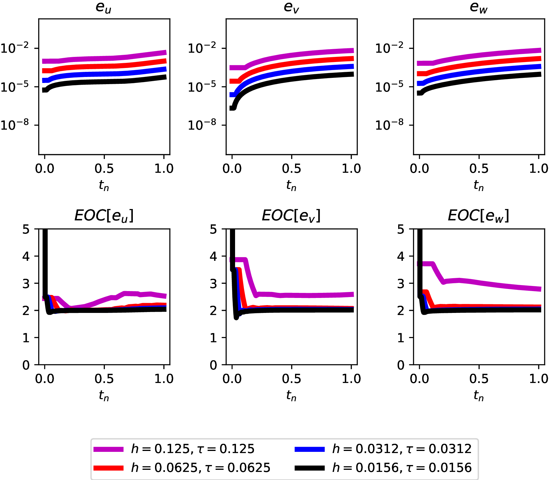
((c)) $q=0$ and $p=3$

((d)) $q=1$ and $p=1$

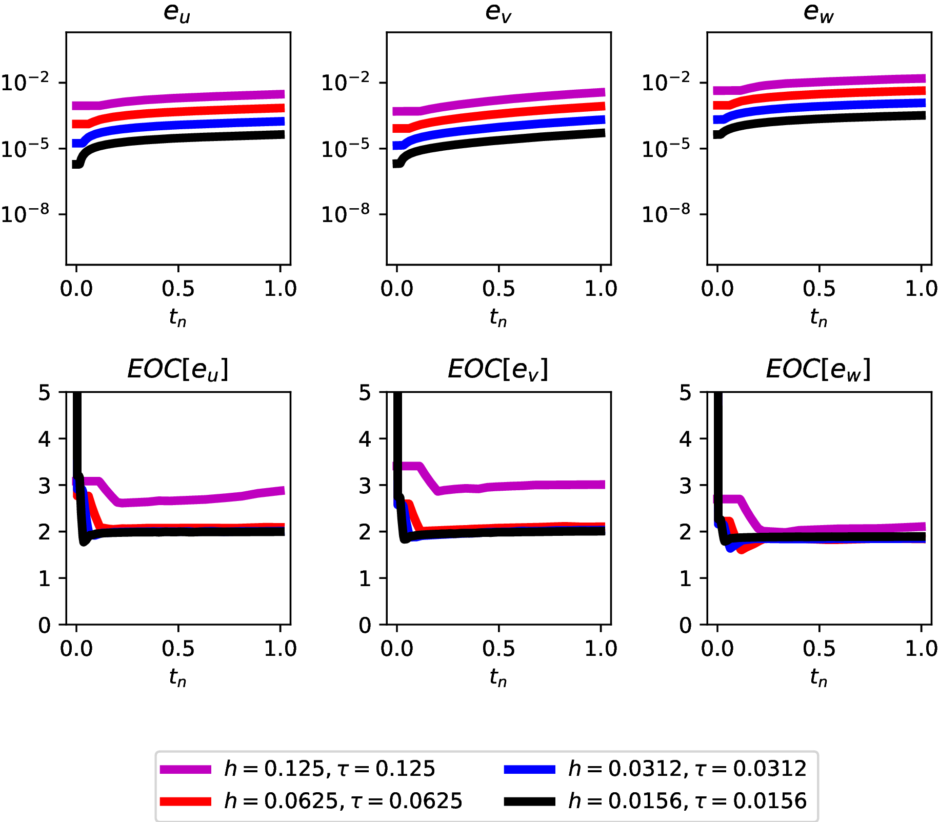
((e)) $q=1$ and $p=2$

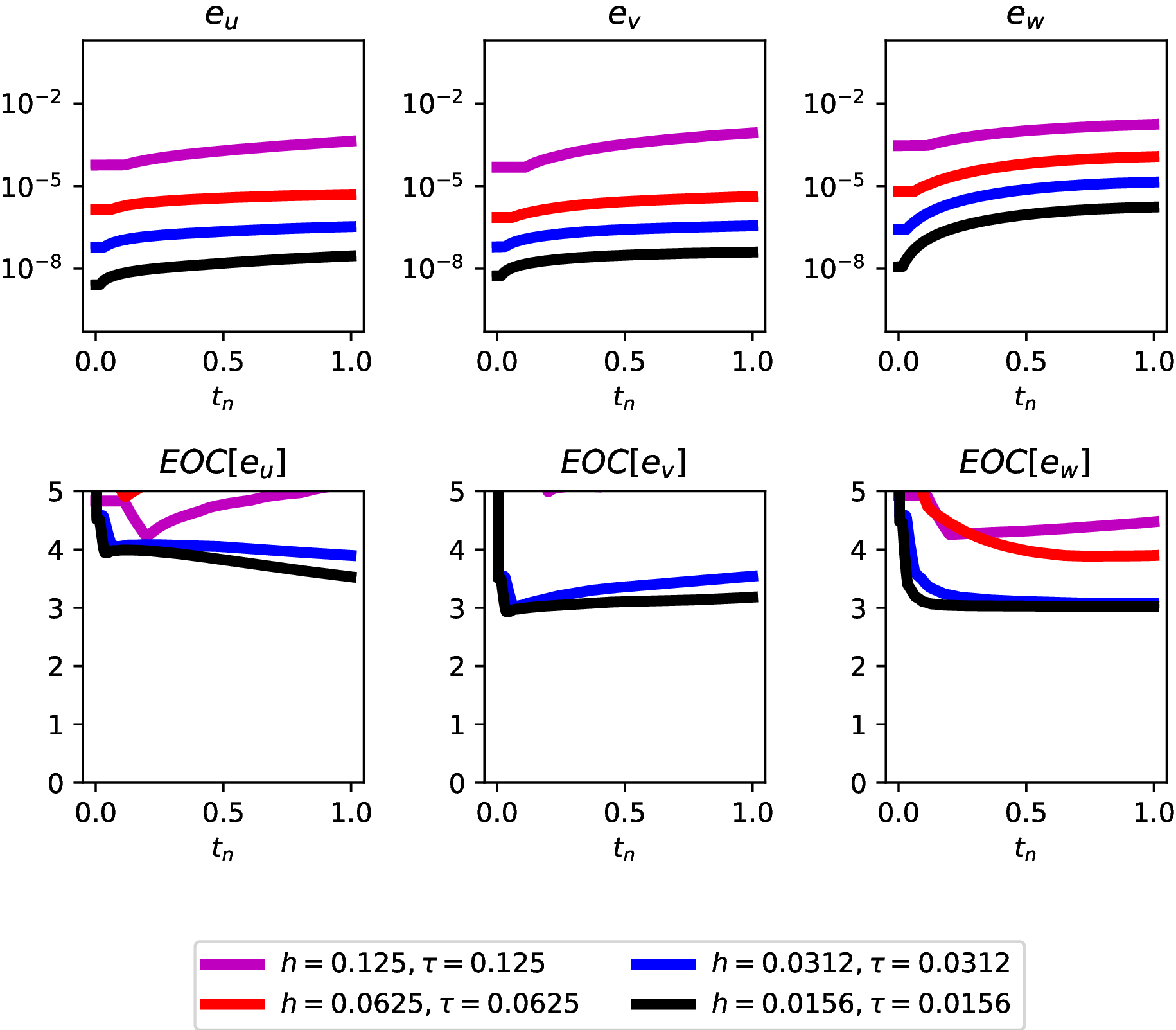
((f)) $q=1$ and $p=3$

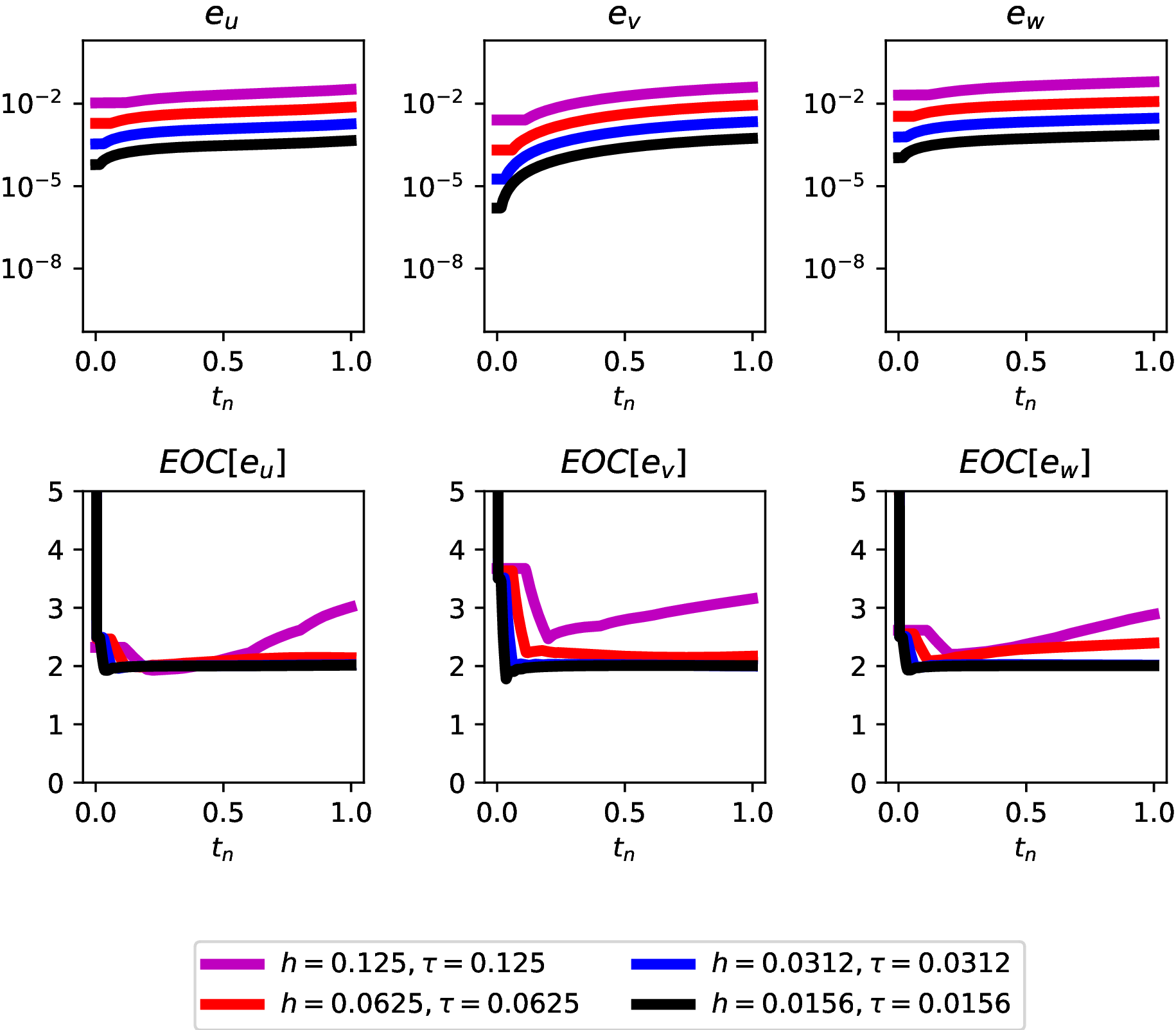
((g)) $q=2$ and $p=1$

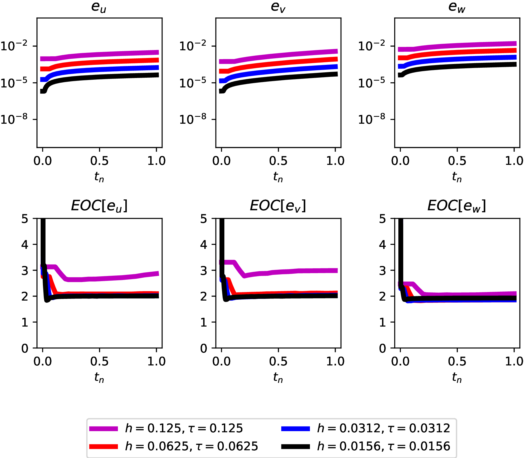
((h)) $q=2$ and $p=2$

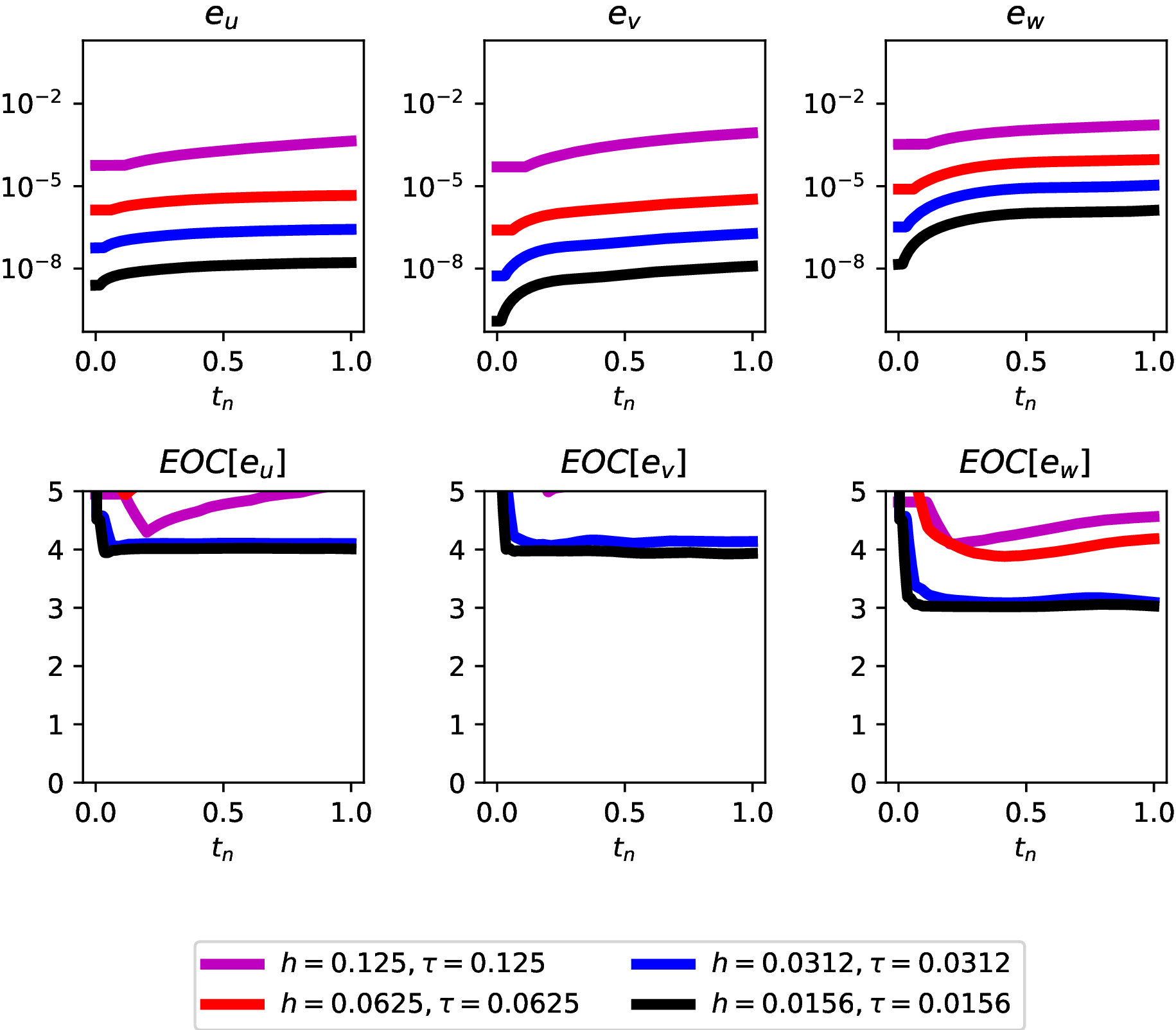
((i)) $q=2$ and $p=3$

Figure 5.5. The error of the spatially continuous finite element scheme (3.6) for the nonlinear Schrödinger equation (5.11) initialised by the exact solution (5.12). Here $e_{u},e_{v},e_{w}$ denotes the errors in the components $U,V,W$ measured in the Bochner norm (5.2). Below we plot the EOC (5.1) corresponding to each of these errors.

Instead simulating the spatially discontinuous finite element approximation (4.5) we obtain Figure 5.6.

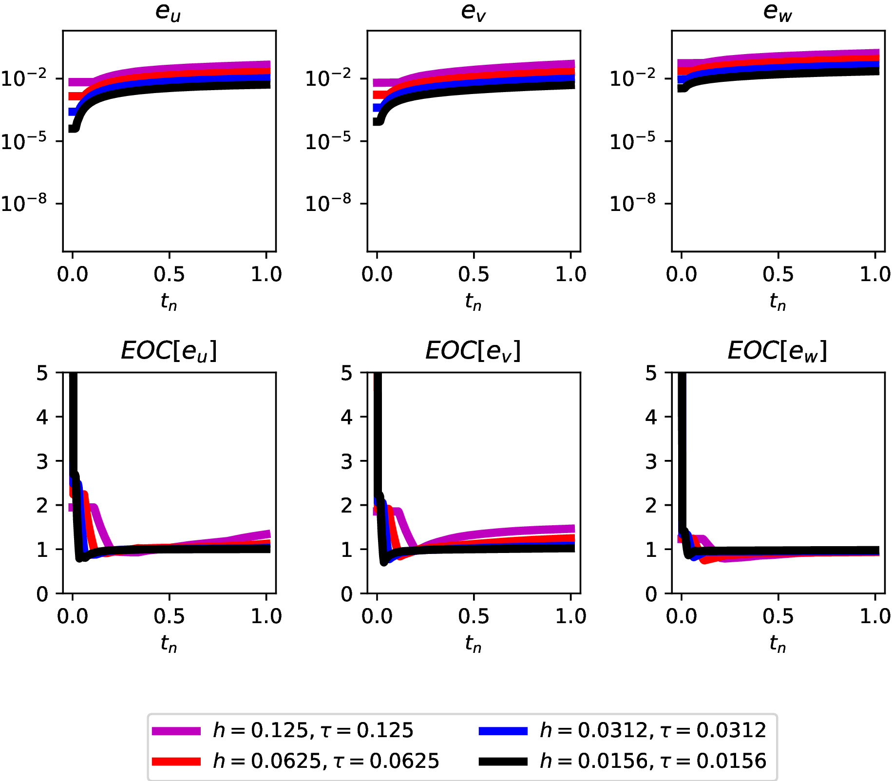
((a)) $q=0$ and $p=1$

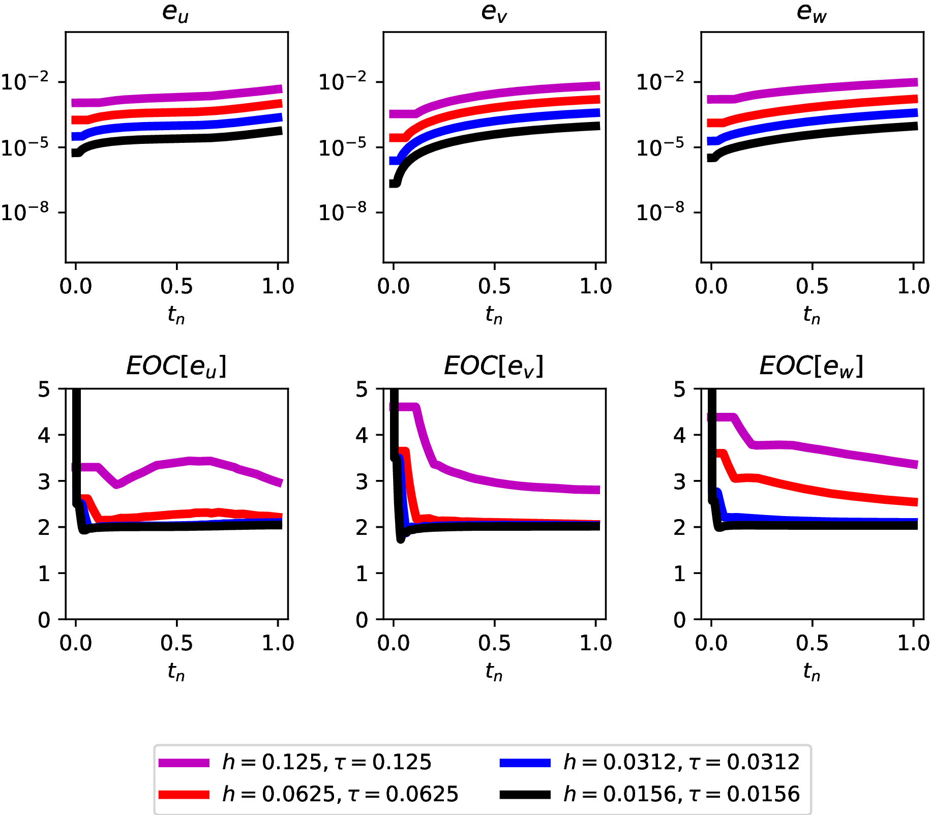
((b)) $q=0$ and $p=2$

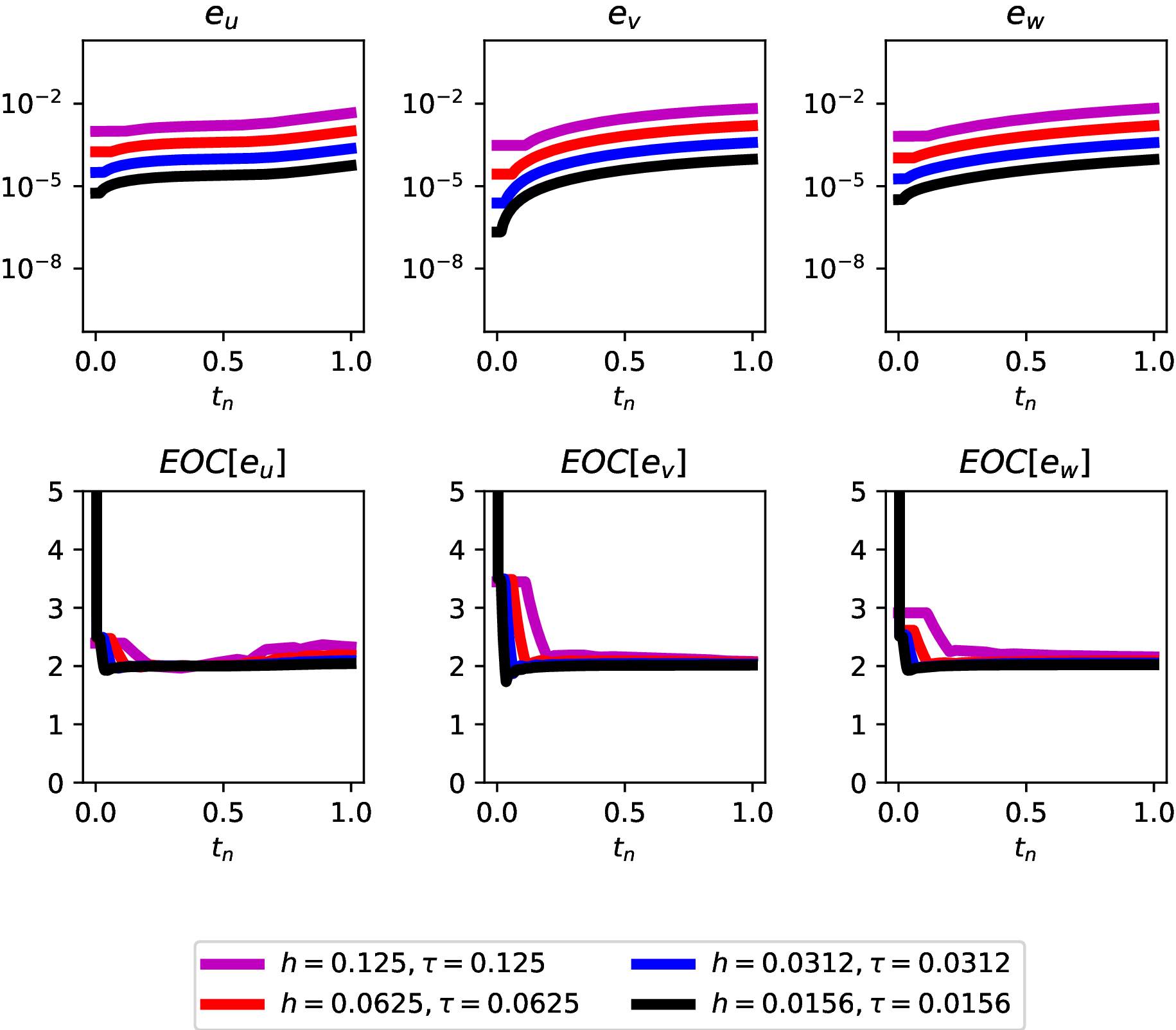
((c)) $q=0$ and $p=3$

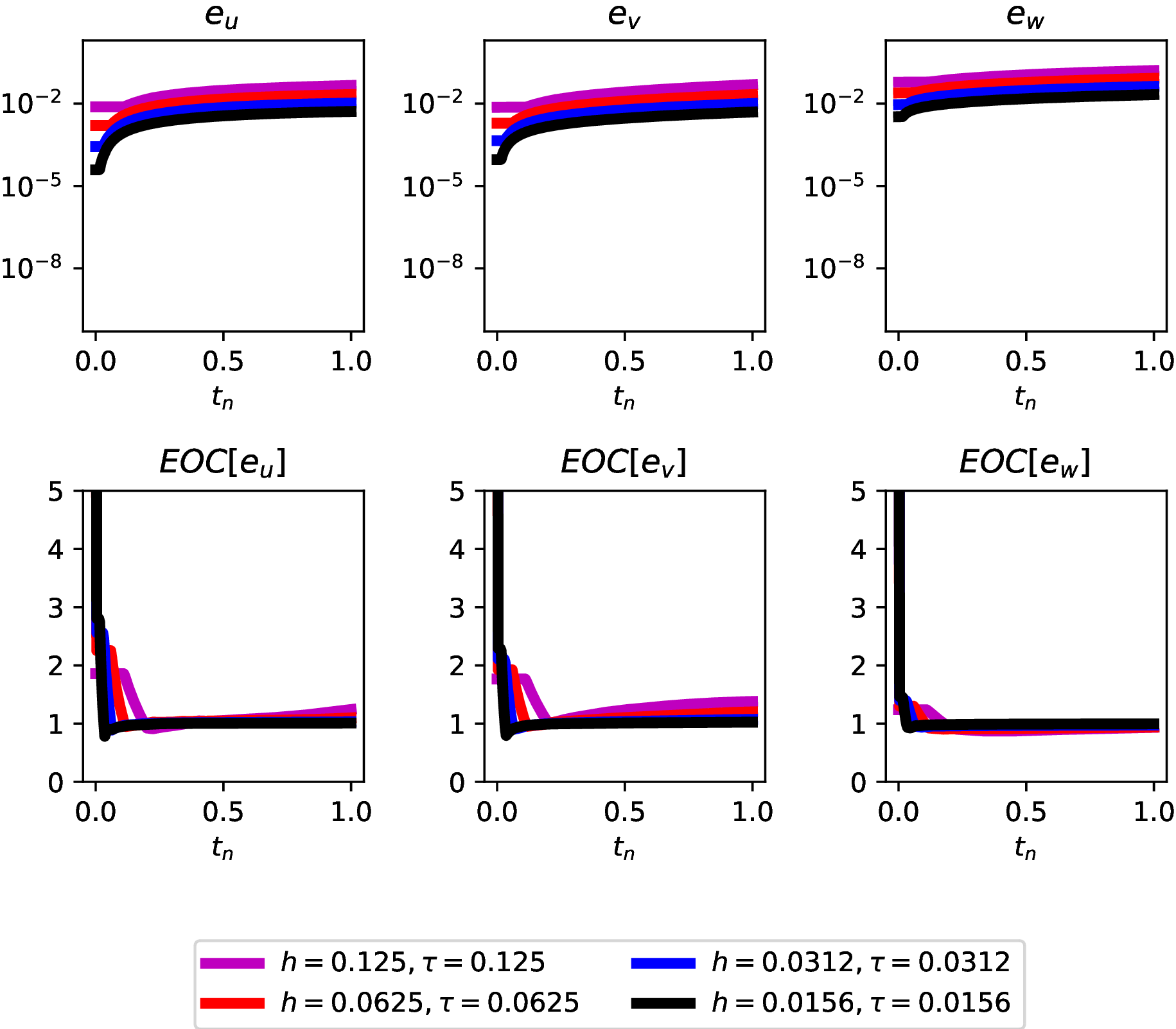
((d)) $q=1$ and $p=1$

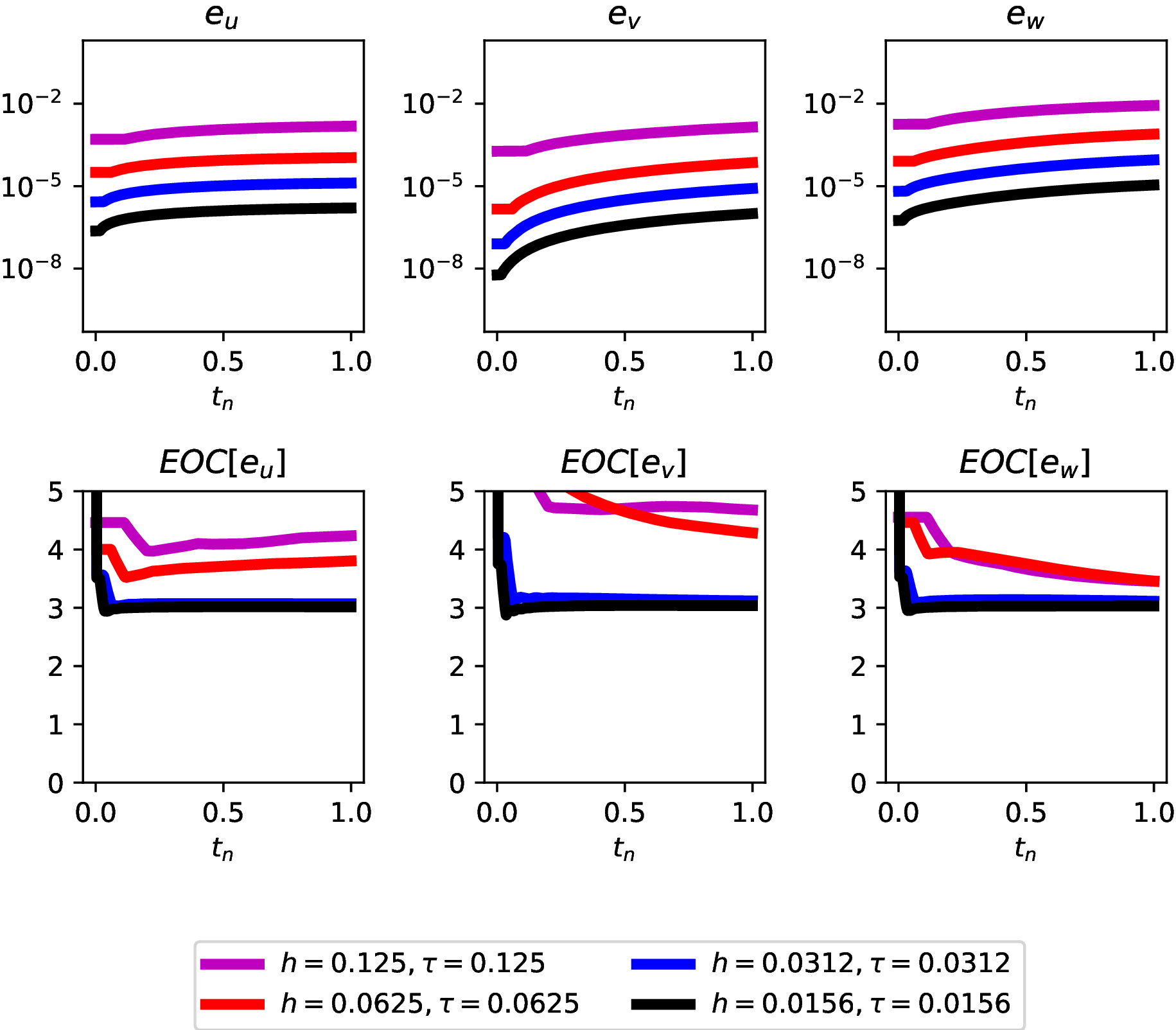
((e)) $q=1$ and $p=2$

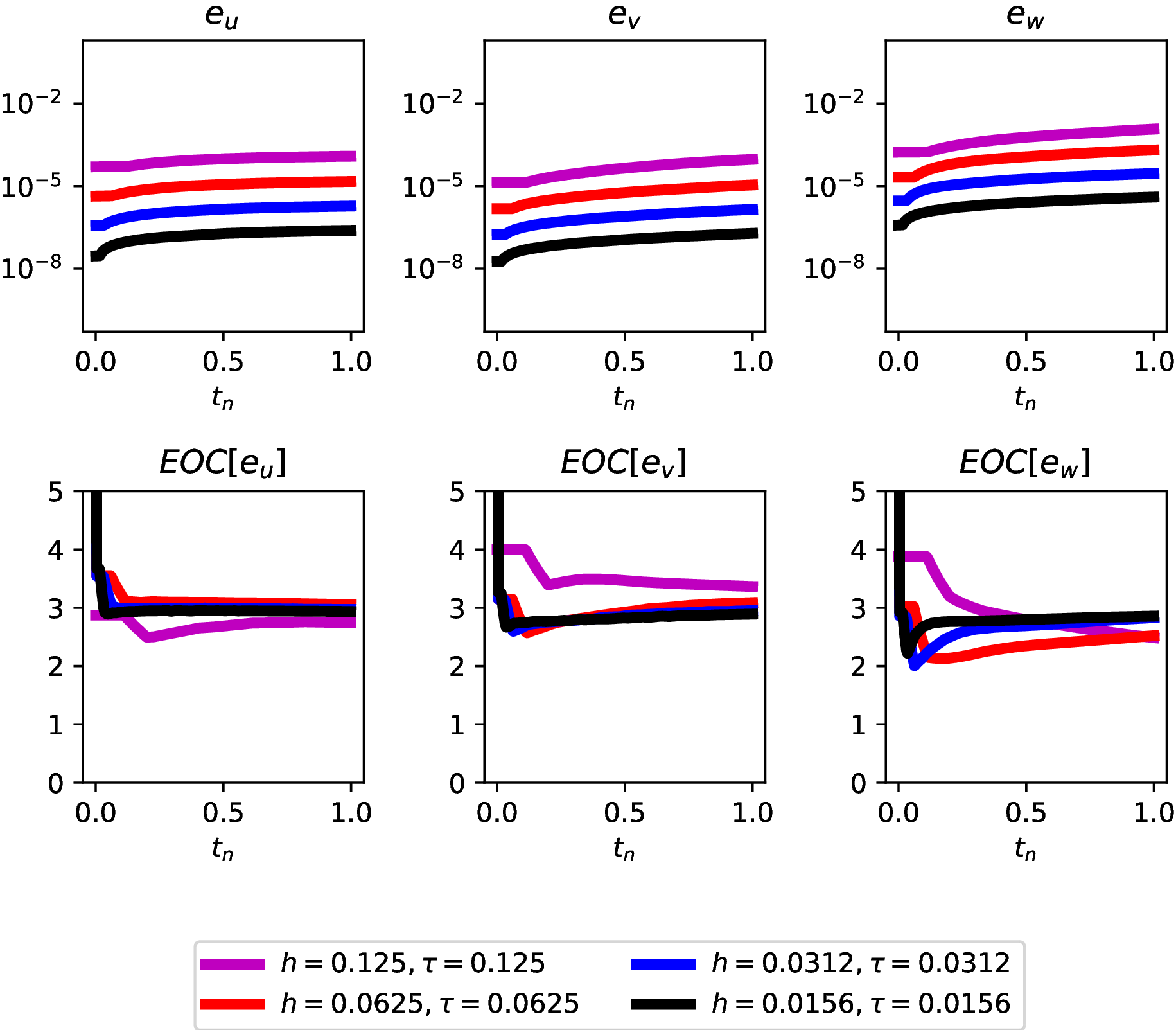
((f)) $q=1$ and $p=3$

((g)) $q=2$ and $p=1$

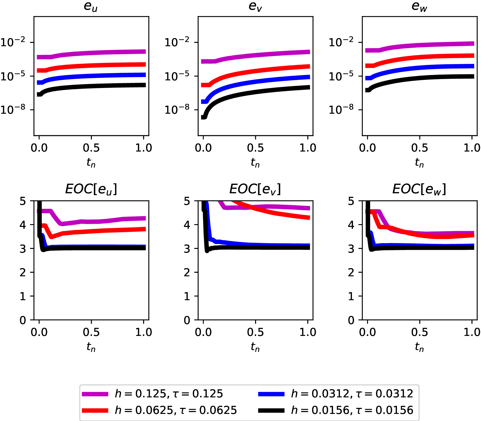
((h)) $q=2$ and $p=2$

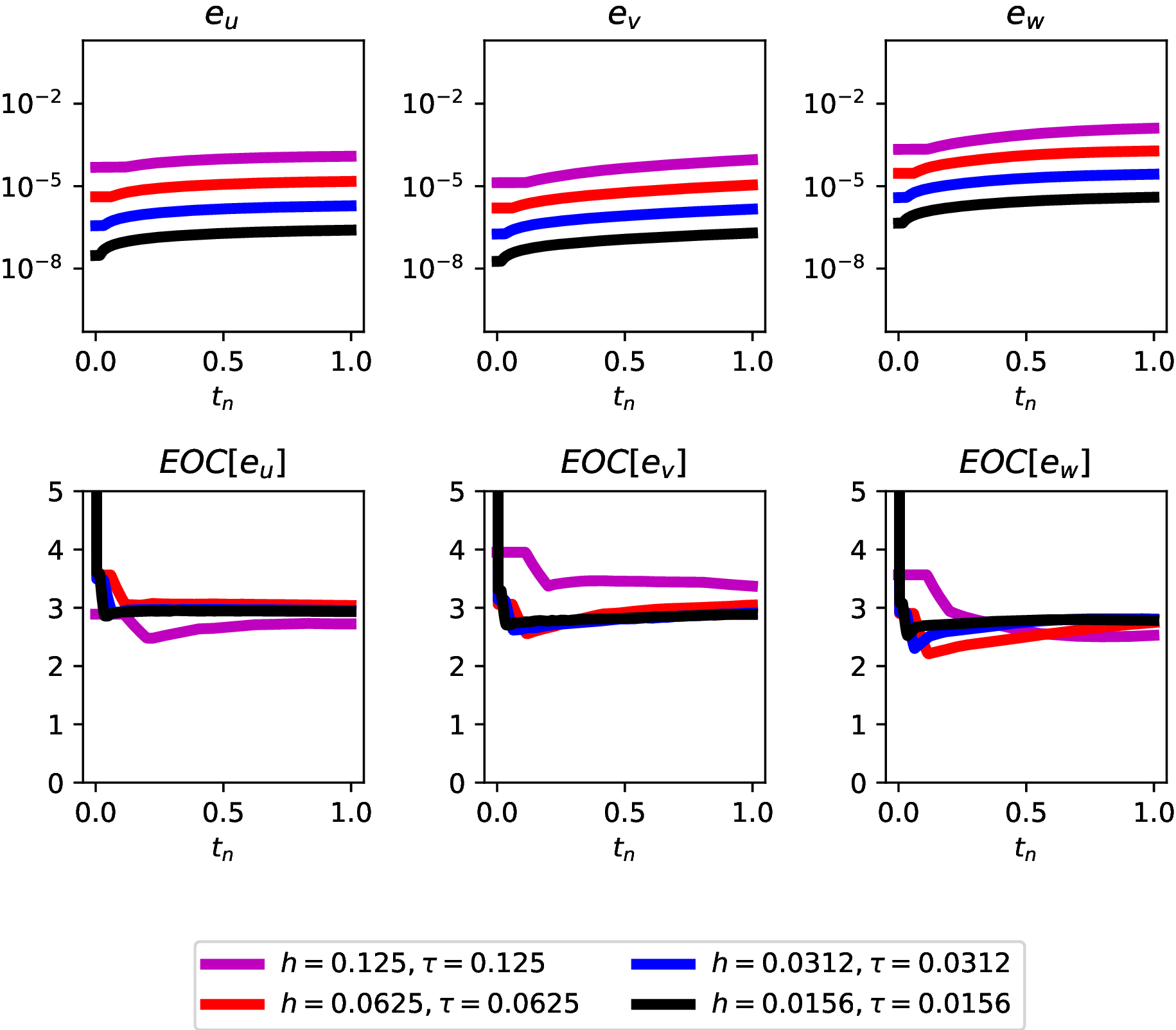
((i)) $q=2$ and $p=3$

Figure 5.6. The error of the spatially discontinuous finite element scheme (4.5) for the nonlinear Schrödinger equation (5.11) initialised by the exact solution (5.12). Here $e_{u},e_{v},e_{w}$ denotes the errors in the components $U,V,W$ measured in the Bochner norm (5.2). Below we plot the EOC (5.1) corresponding to each of these errors.

These simulations further support numerical results we found for the linear wave equation.

Through fixing $\tau=0.1$ and $h=0.04$ we may conduct extensive numerical simulations investigating the deviation in momentum and energy conservation laws. Aforementioned simulations for the spatially continuous approximation (3.6) yield Figure 5.7.

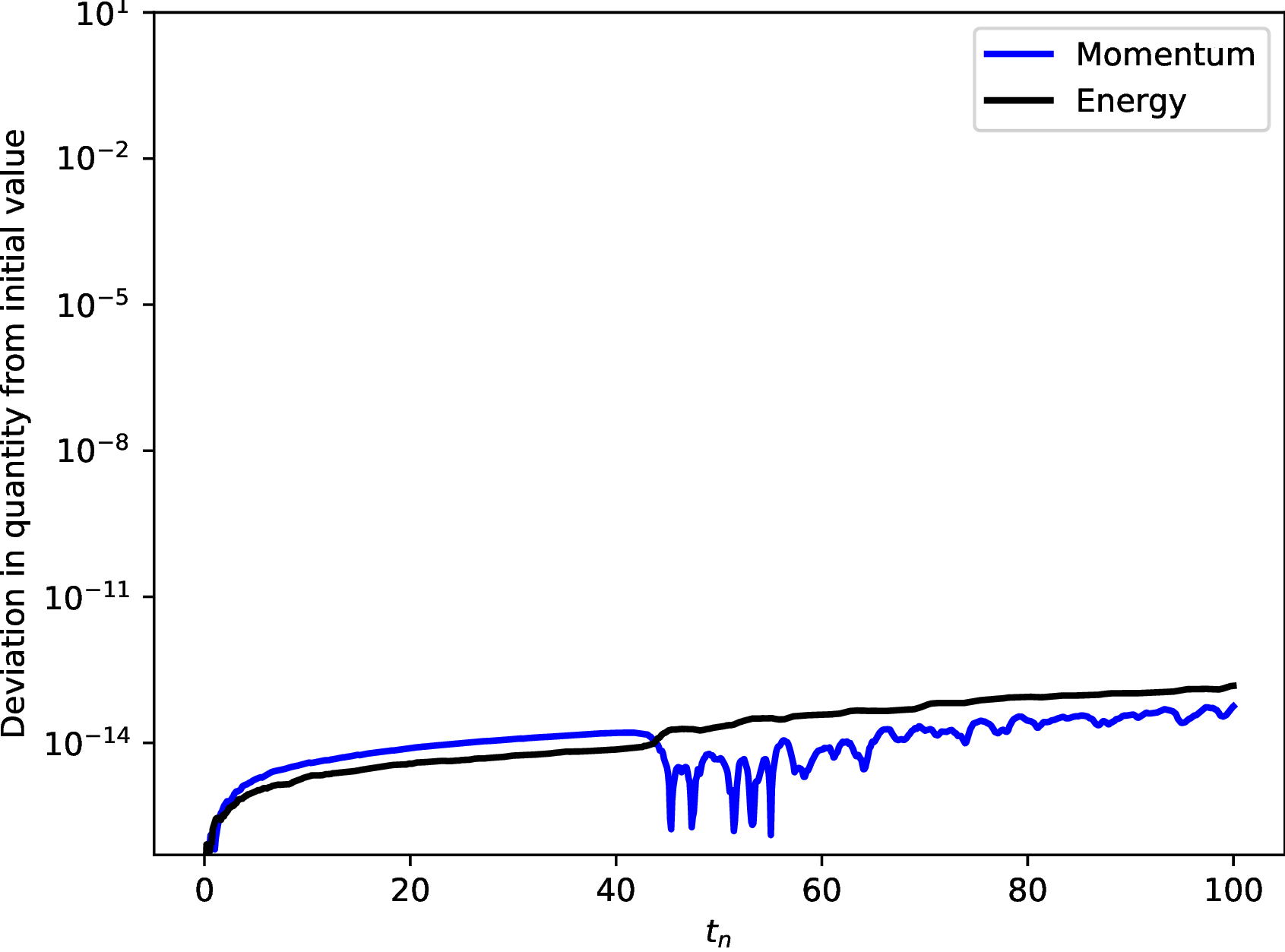
((a)) $q=0$ and $p=1$

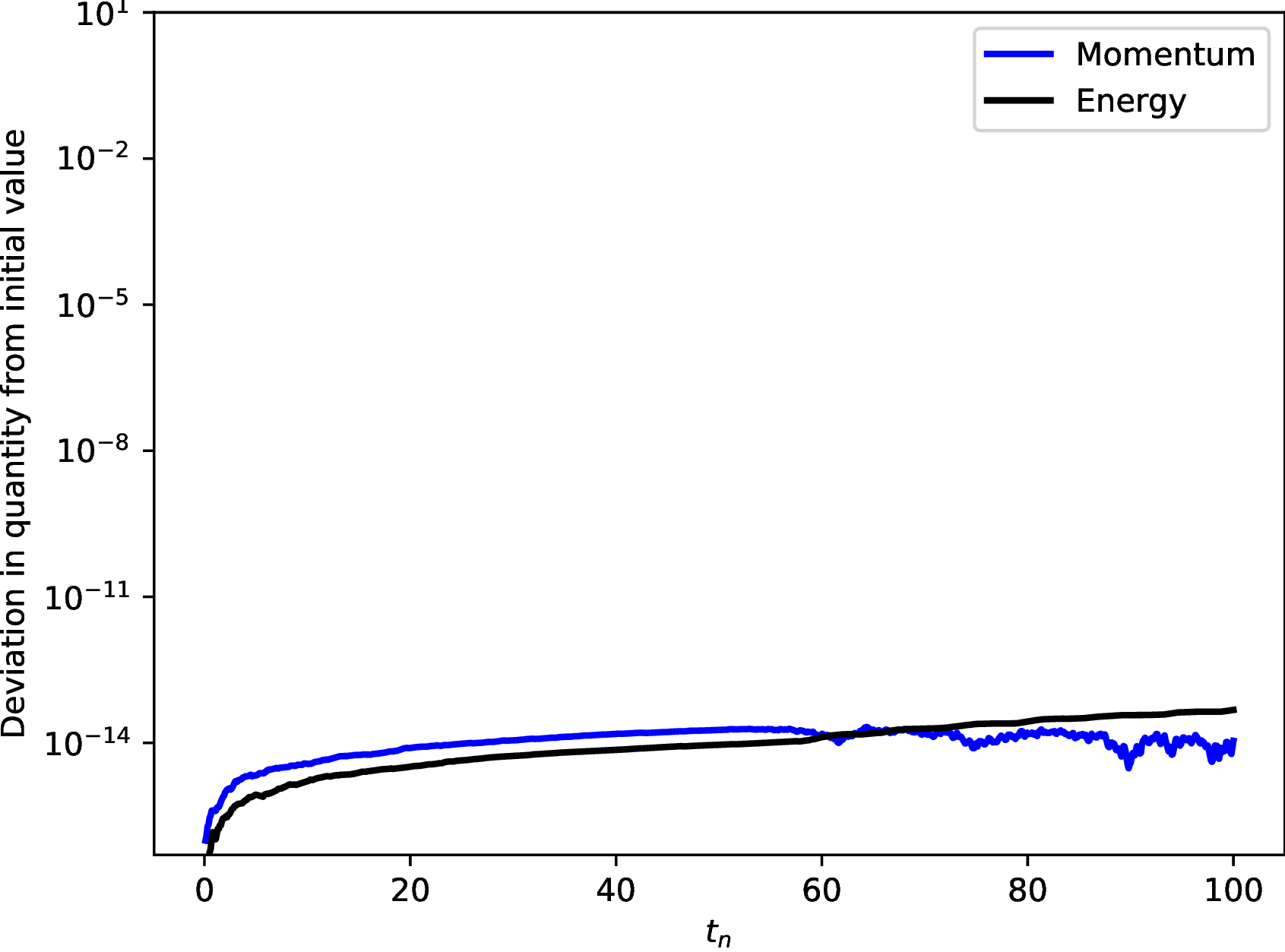
((b)) $q=0$ and $p=2$

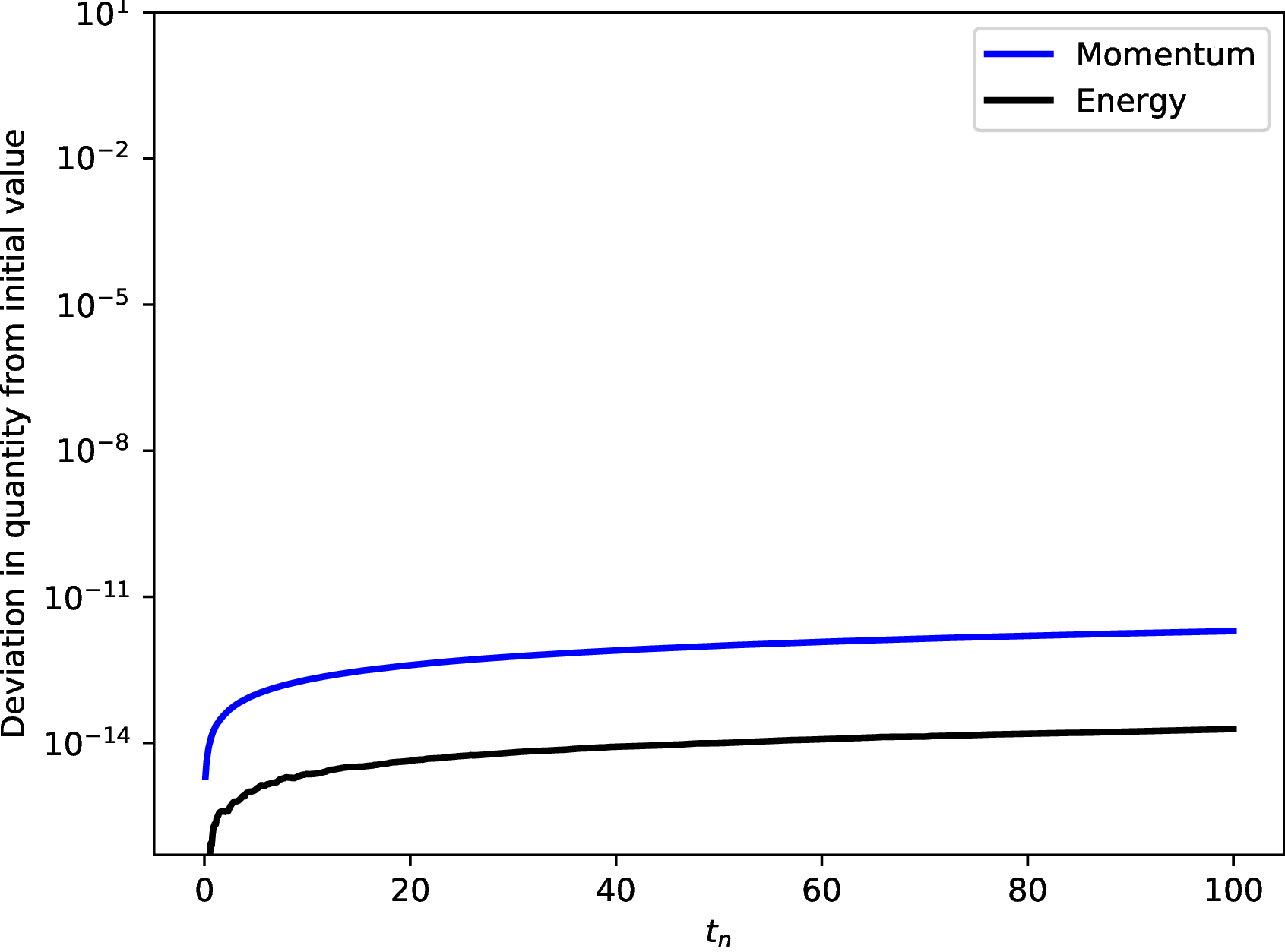
((c)) $q=0$ and $p=3$

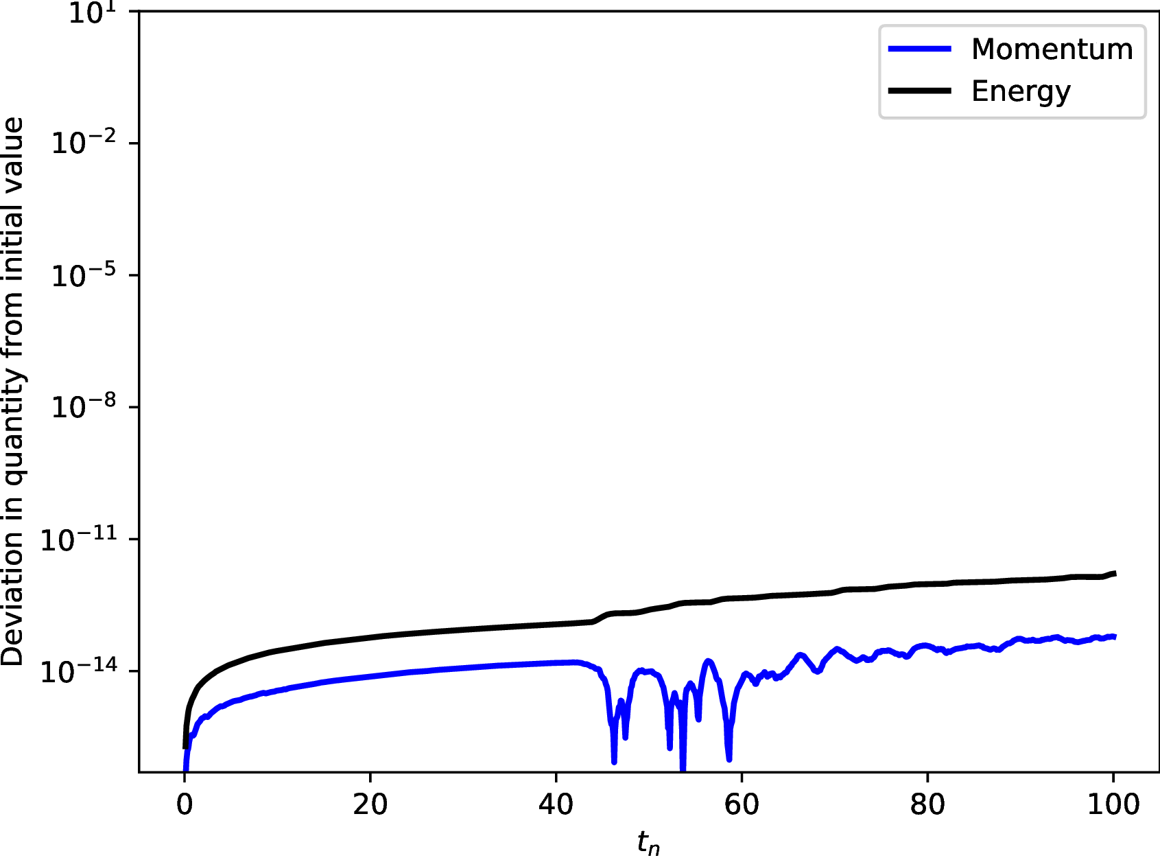
((d)) $q=1$ and $p=1$

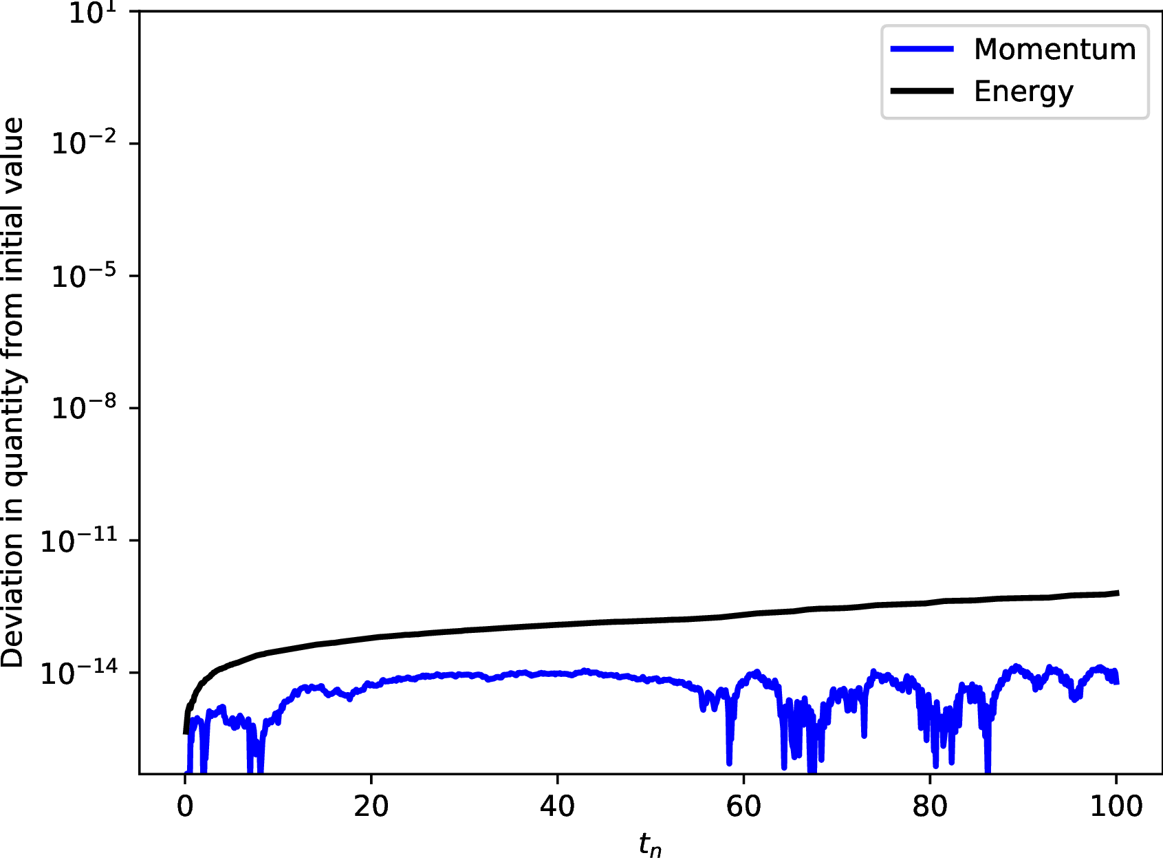
((e)) $q=1$ and $p=2$

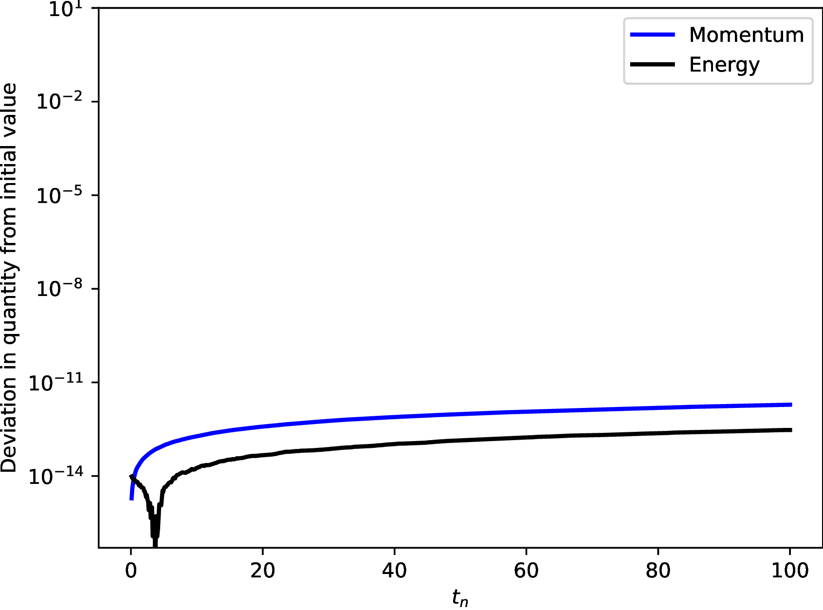
((f)) $q=1$ and $p=3$

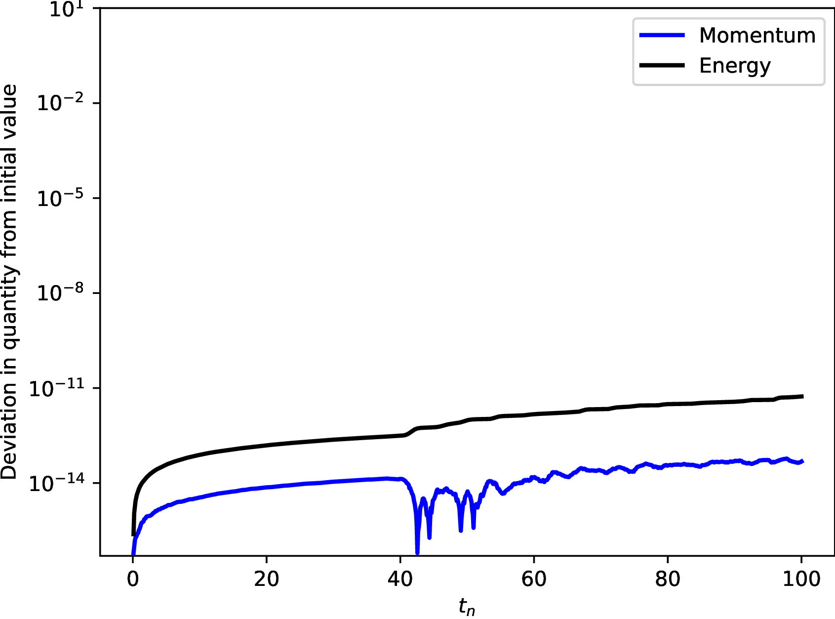
((g)) $q=2$ and $p=1$

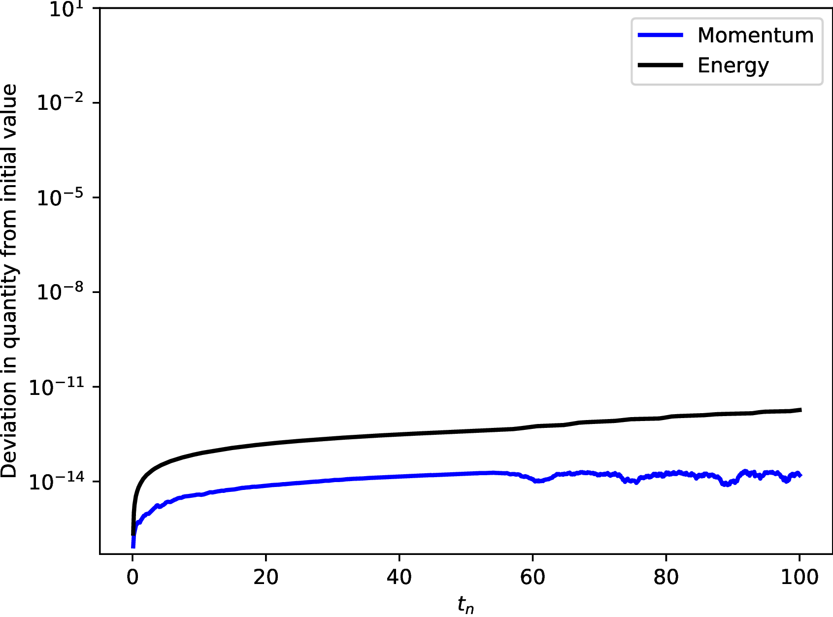
((h)) $q=2$ and $p=2$

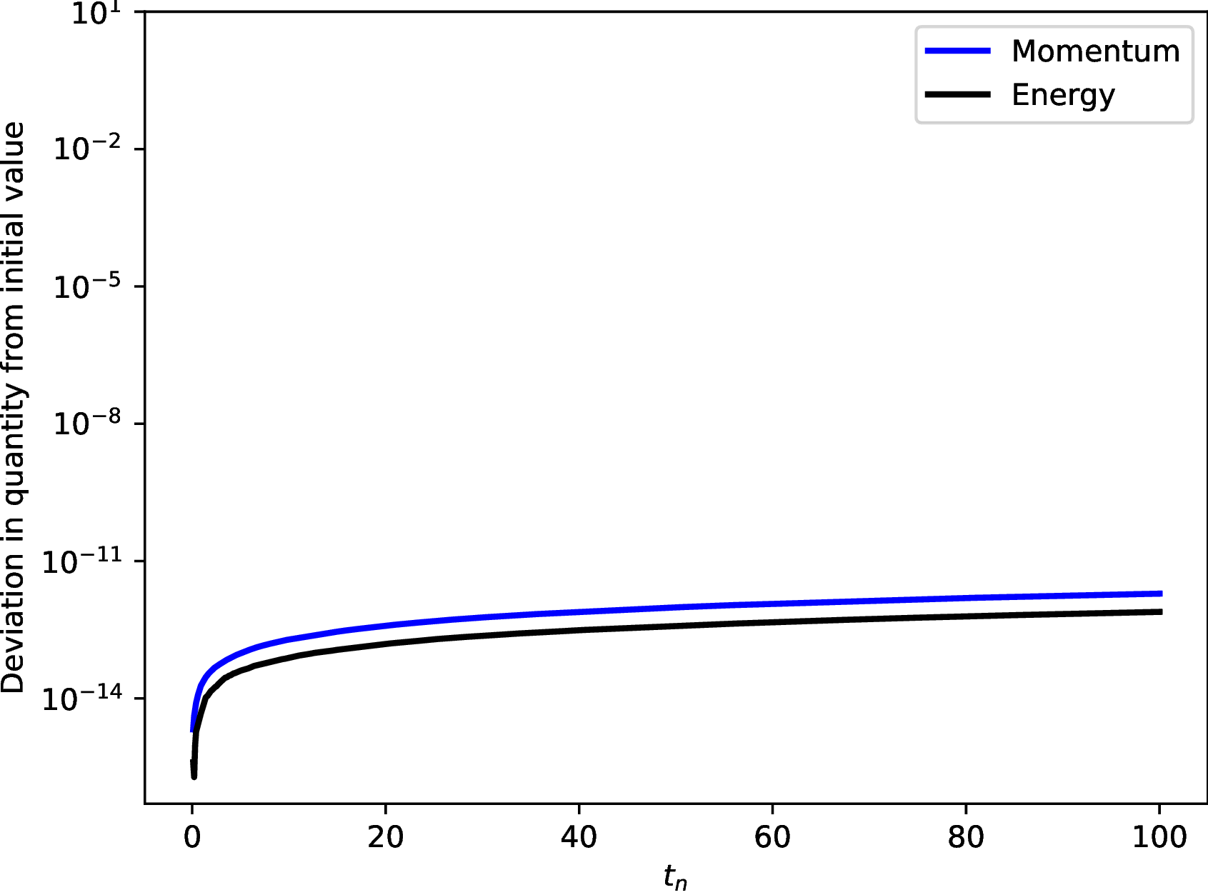
((i)) $q=2$ and $p=3$

Figure 5.7. The deviation in the conservation laws (5.5) and (5.6) for the spatially continuous finite element scheme (3.6) for the NLS equation (5.11) initialised by (5.12) with varying temporal degree $q$ and spatial degree $p$. All simulations have uniform temporal and spatial elements with $\tau=0.1$ and $h=0.4$. We notice that both momentum and energy are preserved below our solver tolerance in all simulations.

We observe in Figure 5.7 that the energy is preserved locally, with the deviation in the energy propagating over time. Furthermore, we note that the momentum is also preserved, which is not analytically guaranteed. We note that we may exactly preserve the momentum here as the consistent momentum conservation law (3.10) is equal to the true momentum conservation law (5.3) up to solver precision. This is, in part, due to the non-linearity in the NLS equation being of low order.

Running the same experiment for the spatially discontinuous scheme (4.5) we obtain Figure 5.8.

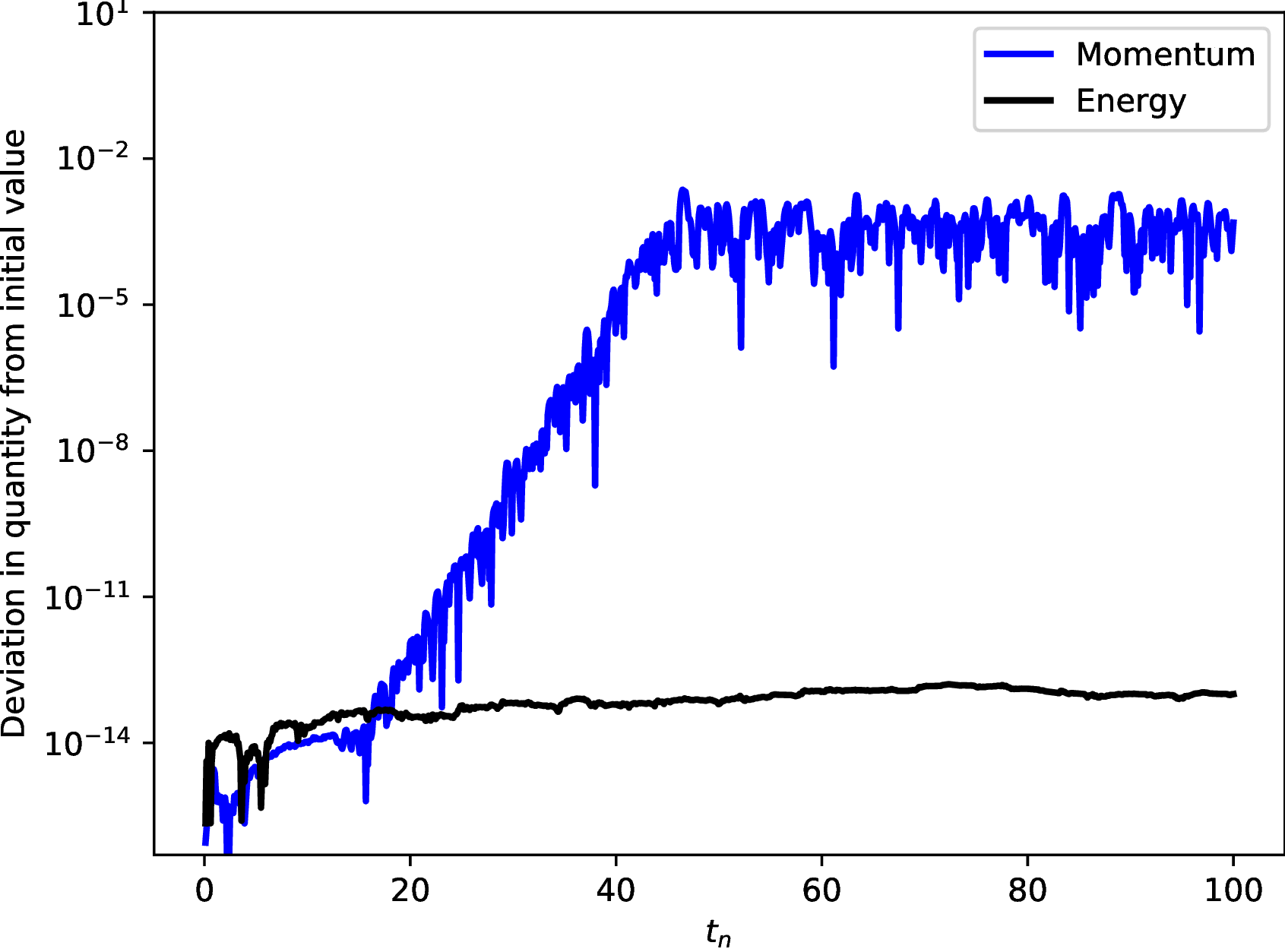
((a)) $q=0$ and $p=1$

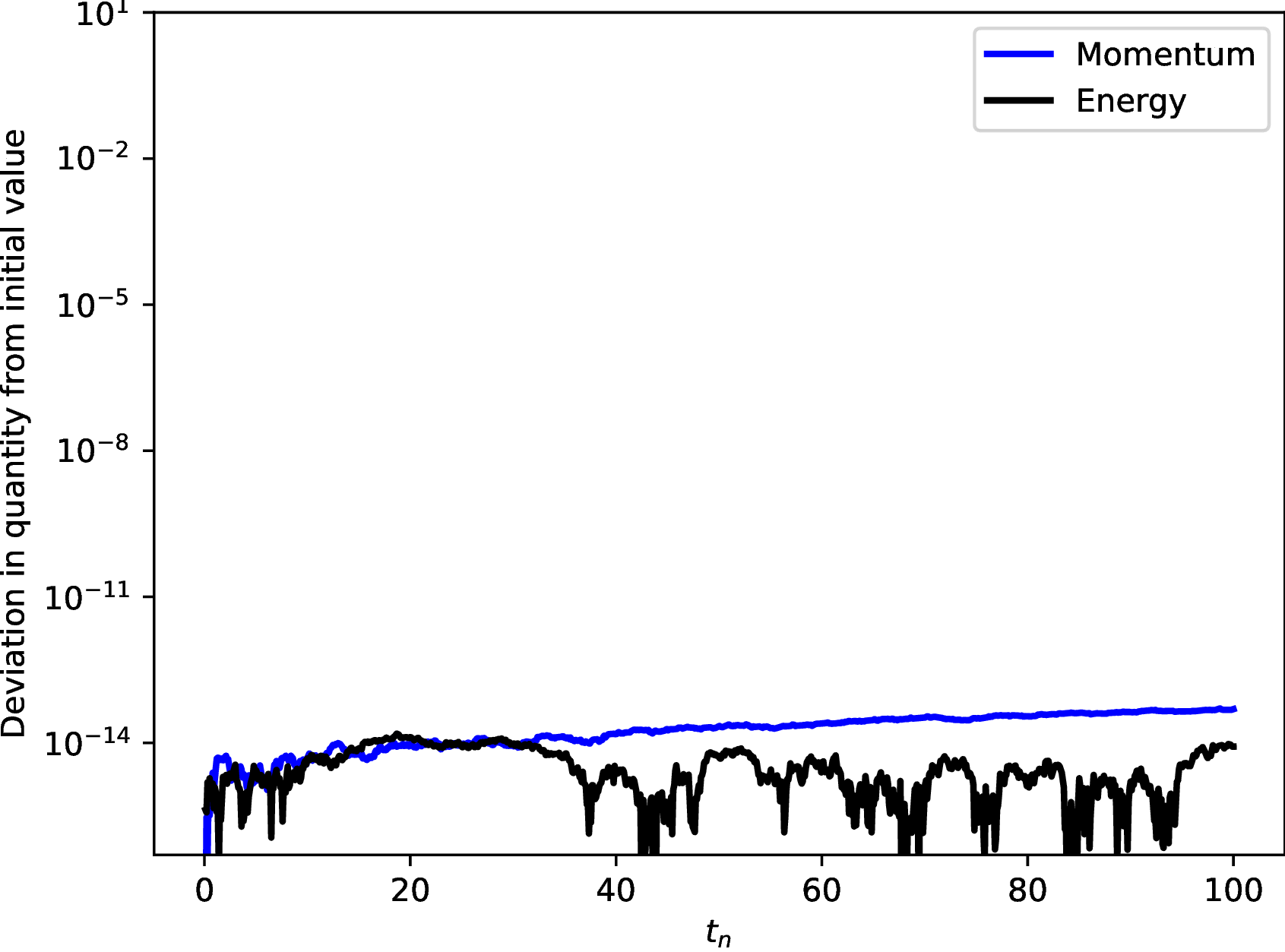
((b)) $q=0$ and $p=2$

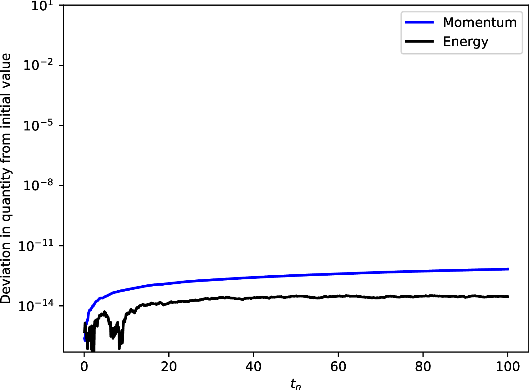
((c)) $q=0$ and $p=3$

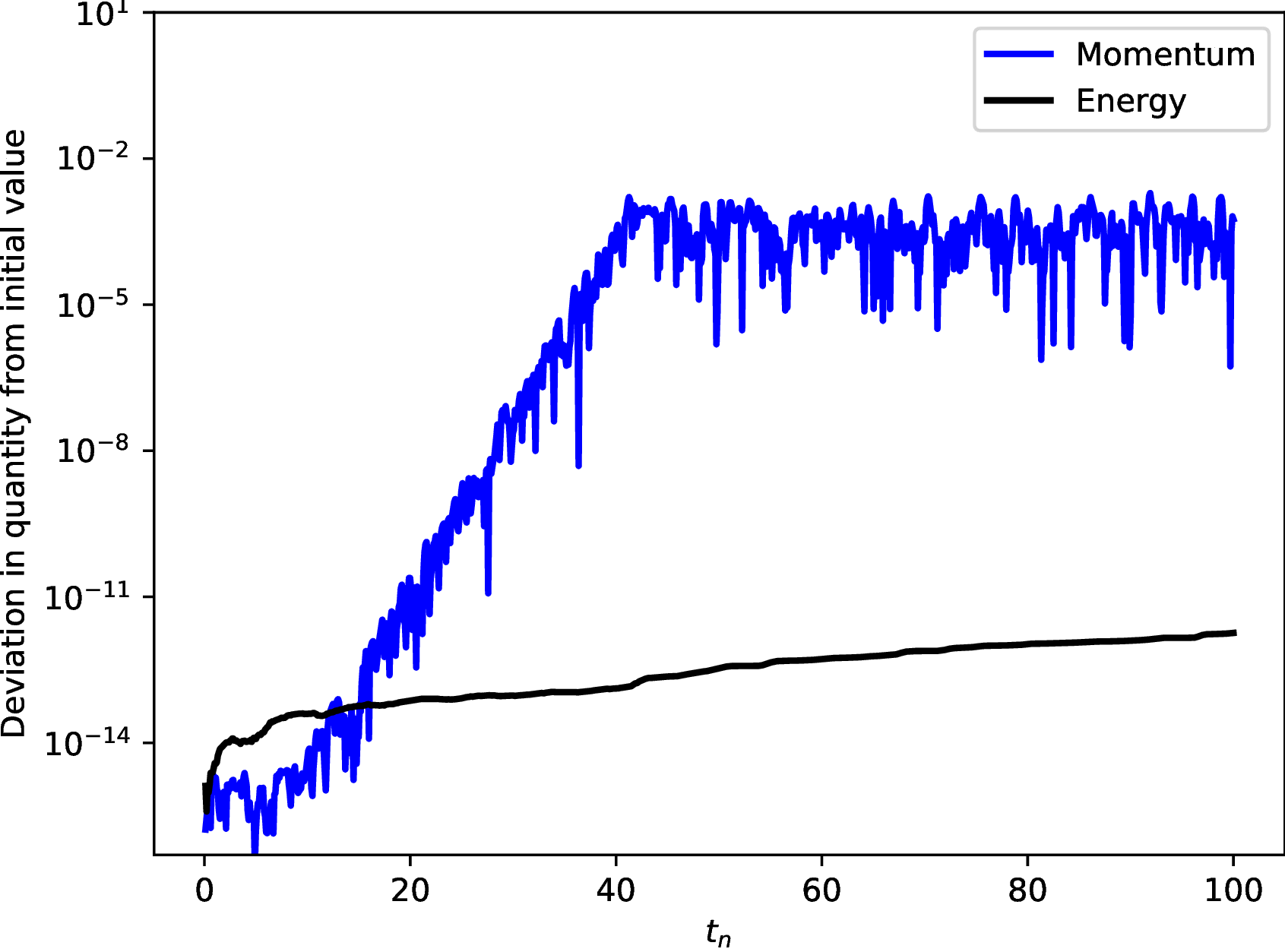
((d)) $q=1$ and $p=1$

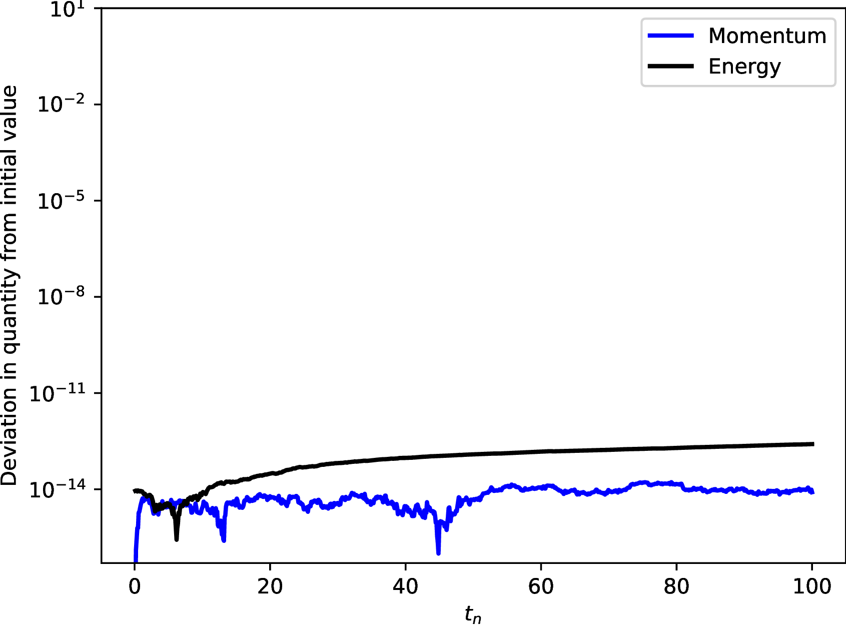
((e)) $q=1$ and $p=2$

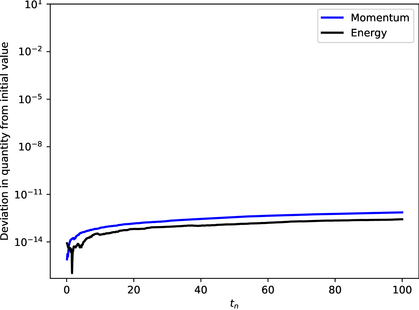
((f)) $q=1$ and $p=3$

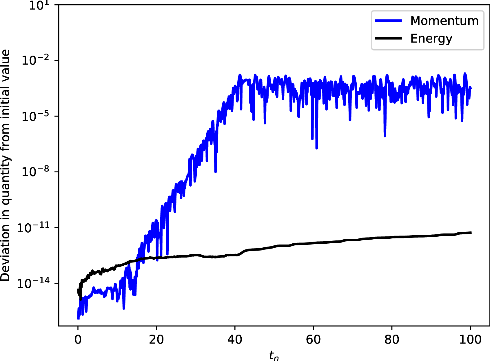
((g)) $q=2$ and $p=1$

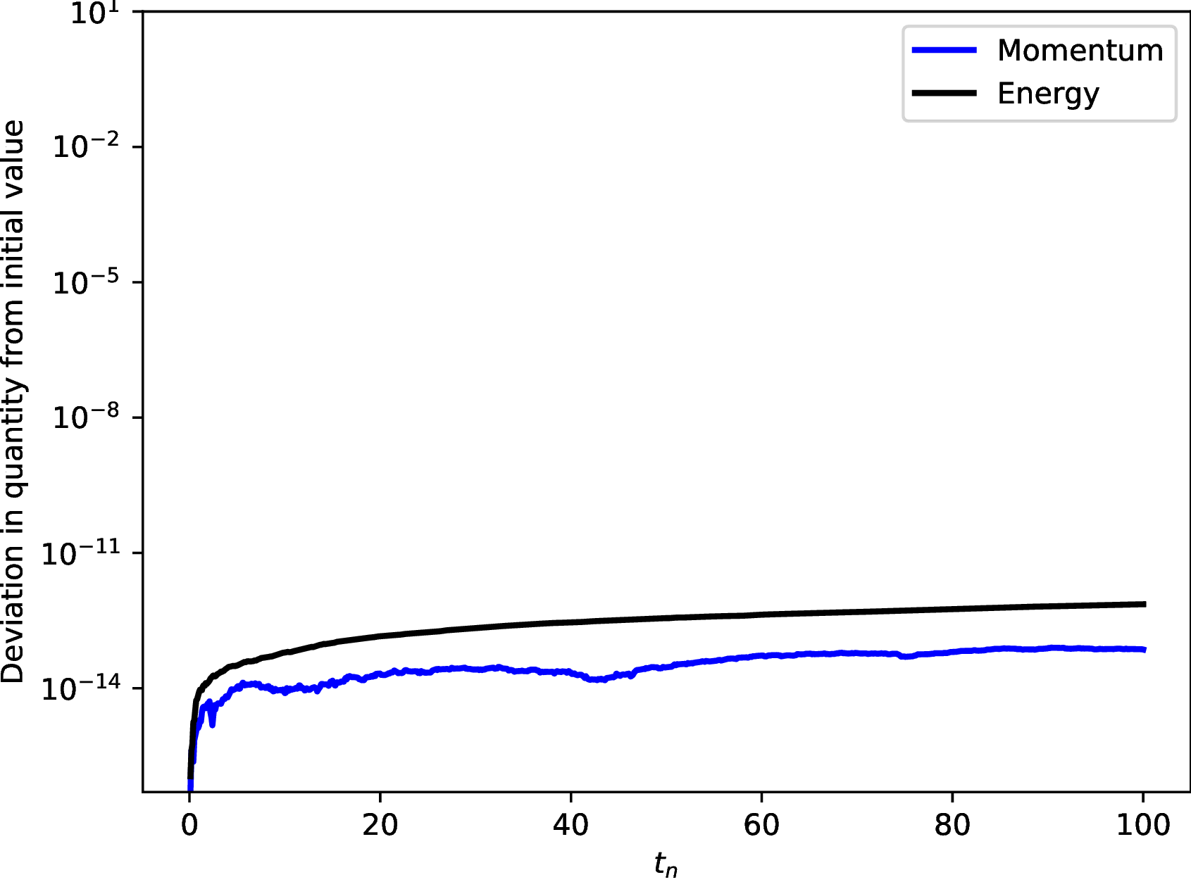
((h)) $q=2$ and $p=2$

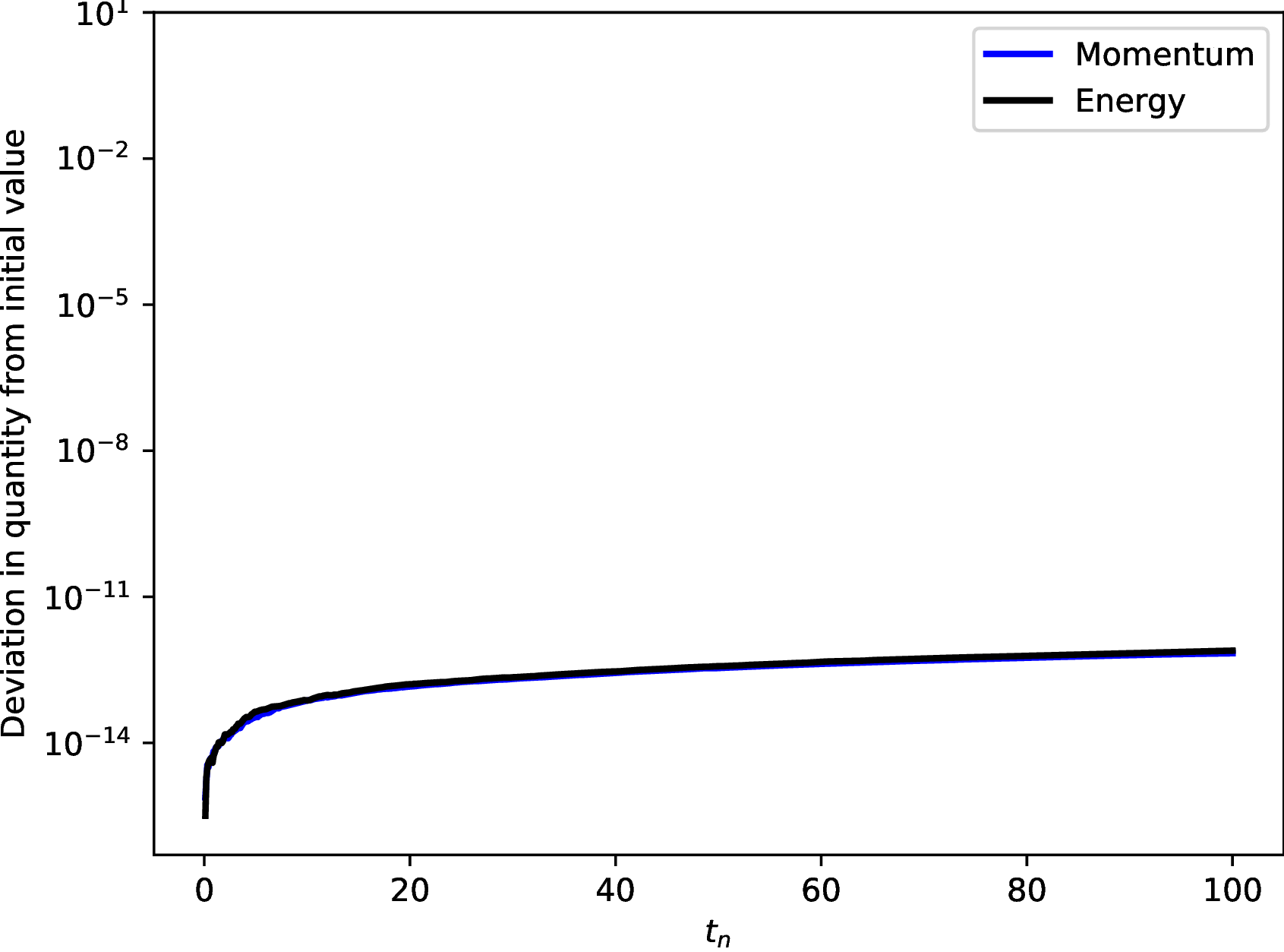
((i)) $q=2$ and $p=3$

Figure 5.8. The deviation in the conservation laws (5.3) and (5.6) for the finite element scheme (3.6) for the NLS equation (5.11) initialised by (5.12) with varying temporal degree $q$ and spatial degree $p$. All simulations have uniform temporal and spatial elements with $\tau=0.1$ and $h=0.04$. We notice that for $p>1$ all laws are preserved below machine precision. For $p=1$ the deviation in momentum propagates significantly over time.

We note that the energy (5.6) is exactly conserved locally with errors propagating over time, however, the momentum (5.3) is not preserved locally unless $p>1$. We note if considering the momentum conserving scheme (3.25), while the momentum would be well preserved the deviation in energy would be large for all $p$.

6. Conclusion

We introduced space-time finite element approximations which preserve geometric structure, namely the energy conservation law, of an arbitrary parabolic multisymplectic PDE. Furthermore we proved existence and uniqueness of this approximation for the wave equation, followed by an extensive numerical study showing good long term behaviour of the solution and convergence of the simulations. Experimentally, the approximations converged optimally in time, with sub-optimal spatial behaviour for both discretisations considered. Our approximation facilitates discretisations over general space-time tensor product domains, and may be readily implemented on nonuniform meshes shaped by an appropriate mesh density function or a posteriori indicator. Furthermore, our methods may be naturally extended to multisymplectic PDEs of a higher spatial dimension, allowing for discretisations over irregular domains. In future work, we shall use the proposed discretisation here to inform fully adaptive space-time algorithms which preserve geometric structure.

References

- [1] P. F. Antonietti, I. Mazzieri, N. Dal Santo, and A. Quarteroni. A high-order discontinuous Galerkin approximation to ordinary differential equations with applications to elastodynamics. IMA J. Numer. Anal., 38(4):1709–1734, 2018.
- [2] U. M. Ascher and R. I. McLachlan. Multisymplectic box schemes and the Korteweg-de Vries equation. Appl. Numer. Math., 48(3-4):255–269, 2004. Workshop on Innovative Time Integrators for PDEs.
- [3] A. K. Aziz and P. Monk. Continuous finite elements in space and time for the heat equation. Math. Comp., 52(186):255–274, 1989.
- [4] S. Balay, S. Abhyankar, M. F. Adams, J. Brown, P. Brune, K. Buschelman, L. Dalcin, V. Eijkhout, W. D. Gropp, D. Kaushik, M. G. Knepley, D. A. May, L. C. McInnes, R. T. Mills, T. Munson, K. Rupp, P. Sanan, B. F. Smith, S. Zampini, H. Zhang, and H. Zhang. PETSc users manual. Technical Report ANL-95/11 - Revision 3.9, Argonne National Laboratory, 2018.
- [5] L. Beirão da Veiga, L. Lopez, and G. Vacca. Mimetic finite difference methods for Hamiltonian wave equations in 2D. Comput. Math. Appl., 74(5):1123–1141, 2017.
- [6] G.-T. Bercea, A. T. McRae, D. A. Ham, L. Mitchell, F. Rathgeber, L. Nardi, F. Luporini, and P. H. Kelly. A structure-exploiting numbering algorithm for finite elements on extruded meshes, and its performance evaluation in Firedrake. arXiv preprint arXiv:1604.05937, 2016.
- [7] P. Betsch and P. Steinmann. Inherently energy conserving time finite elements for classical mechanics. J. Comput. Phys., 160(1):88–116, 2000.
- [8] A. Bihlo, J. Jackaman, and F. Valiquette. On the development of symmetry preserving finite element schemes for ordinary differential equations. Journal of Computational Dynamics (in review), 2019.
- [9] T. J. Bridges. Multi-symplectic structures and wave propagation. Math. Proc. Cambridge Philos. Soc., 121(1):147–190, 1997.
- [10] T. J. Bridges and S. Reich. Multi-symplectic integrators: numerical schemes for Hamiltonian PDEs that conserve symplecticity. Phys. Lett. A, 284(4-5):184–193, 2001.
- [11] S. Buchholz, B. Dörich, and M. Hochbruck. On averaged exponential integrators for semilinear wave equations with solutions of low-regularity. Technical Report 8, Karlsruher Institut für Technologie (KIT), 2020.
- [12] S. Buchholz, L. Gauckler, V. Grimm, M. Hochbruck, and T. Jahnke. Closing the gap between trigonometric integrators and splitting methods for highly oscillatory differential equations. IMA J. Numer. Anal., 38(1):57–74, 2018.
- [13] B. Cano. Conserved quantities of some Hamiltonian wave equations after full discretization. Numer. Math., 103(2):197–223, 2006.
- [14] P. Castillo. A review of the local discontinuous Galerkin (LDG) method applied to elliptic problems. Appl. Numer. Math., 56(10-11):1307–1313, 2006.
- [15] P. Castillo, B. Cockburn, I. Perugia, and D. Schötzau. An a priori error analysis of the local discontinuous Galerkin method for elliptic problems. SIAM J. Numer. Anal., 38(5):1676–1706, 2000.
- [16] P. Castillo and S. Gómez. On the conservation of fractional nonlinear Schrödinger equation’s invariants by the local discontinuous Galerkin method. J. Sci. Comput., 77(3):1444–1467, 2018.
- [17] E. Celledoni, V. Grimm, R. I. McLachlan, D. I. McLaren, D. O’Neale, B. Owren, and G. R. W. Quispel. Preserving energy resp. dissipation in numerical PDEs using the “average vector field” method. J. Comput. Phys., 231(20):6770–6789, 2012.
- [18] B. Cockburn and J. Gopalakrishnan. A characterization of hybridized mixed methods for second order elliptic problems. SIAM J. Numer. Anal., 42(1):283–301, 2004.
- [19] B. Cockburn, J. Gopalakrishnan, and R. Lazarov. Unified hybridization of discontinuous Galerkin, mixed, and continuous Galerkin methods for second order elliptic problems. SIAM J. Numer. Anal., 47(2):1319–1365, 2009.
- [20] B. Cockburn and C.-W. Shu. The Runge-Kutta discontinuous Galerkin method for conservation laws. V. Multidimensional systems. J. Comput. Phys., 141(2):199–224, 1998.
- [21] R. Courant, K. Friedrichs, and H. Lewy. On the partial difference equations of mathematical physics. IBM J. Res. Develop., 11:215–234, 1967.
- [22] D. Estep. A posteriori error bounds and global error control for approximation of ordinary differential equations. SIAM J. Numer. Anal., 32(1):1–48, 1995.
- [23] D. Estep and D. French. Global error control for the continuous Galerkin finite element method for ordinary differential equations. RAIRO Modél. Math. Anal. Numér., 28(7):815–852, 1994.
- [24] D. J. Estep and A. M. Stuart. The dynamical behavior of the discontinuous Galerkin method and related difference schemes. Math. Comp., 71(239):1075–1103, 2002.
- [25] D. A. French and J. W. Schaeffer. Continuous finite element methods which preserve energy properties for nonlinear problems. Appl. Math. Comput., 39(3):271–295, 1990.
- [26] I. Fried. Finite-element analysis of time-dependent phenomena. AIAA Journal, 7(6):1170–1173, 1969.
- [27] J. Giesselmann and T. Pryer. Reduced relative entropy techniques for a priori analysis of multiphase problems in elastodynamics. BIT, 56(1):99–127, 2016.
- [28] Y. Gong, J. Cai, and Y. Wang. Some new structure-preserving algorithms for general multi-symplectic formulations of Hamiltonian PDEs. J. Comput. Phys., 279:80–102, 2014.
- [29] E. Hairer, C. Lubich, and G. Wanner. Geometric numerical integration, volume 31 of Springer Series in Computational Mathematics. Springer-Verlag, Berlin, second edition, 2006. Structure-preserving algorithms for ordinary differential equations.
- [30] P. Hansbo. A note on energy conservation for hamiltonian systems using continuous time finite elements. Commun. Numer. Meth. Engng., 17:863–869, 2001.
- [31] A. Islas, D. Karpeev, and C. Schober. Geometric integrators for the nonlinear Schrödinger equation. J. Comput. Phys., 173:116–148, 2001.
- [32] A. L. Islas and C. M. Schober. Backward error analysis for multisymplectic discretizations of Hamiltonian PDEs. Math. Comput. Simulation, 69(3-4):290–303, 2005.
- [33] J. Jackaman. Finite element methods as geometric structure preserving algorithms. PhD thesis, School of Mathematical, Physical and Computational Sciences, University of Reading, 2018.
- [34] J. Jackaman and T. Pryer. Conservative Galerkin methods for dispersive Hamiltonian problems. arXiv preprint arXiv:1811.09999, 2018.
- [35] V. S. K. U. Julian Henning, Davide Palitta. Matrix oriented reduction of space-time Petrov-Galerkin variational problems. arXiv, 2019.
- [36] O. Karakashian and C. Makridakis. A space-time finite element method for the nonlinear Schrödinger equation: the continuous Galerkin method. SIAM J. Numer. Anal., 36(6):1779–1807, 1999.
- [37] J.-L. Lions and E. Magenes. Problèmes aux limites non homogènes et applications. Vol. 1. Travaux et Recherches Mathématiques, No. 17. Dunod, Paris, 1968.
- [38] J. E. Marsden and S. S. George W. Partick. Multisymplectic geometry, variational integrators, and nonlinear pdes. Commun. Math. Phys., 199:351–395, 1998.
- [39] J. E. Marsden and S. Shkoller. Multisymplectic geometry, covariant Hamiltonians, and water waves. Math. Proc. Cambridge Philos. Soc., 125(3):553–575, 1999.
- [40] F. McDonald, R. I. McLachlan, B. E. Moore, and G. R. W. Quispel. Travelling wave solutions of multisymplectic discretizations of semi-linear wave equations. J. Difference Equ. Appl., 22(7):913–940, 2016.
- [41] R. I. McLachlan and G. R. W. Quispel. Discrete gradient methods have an energy conservation law. Discrete Contin. Dyn. Syst., 34(3):1099–1104, 2014.
- [42] R. I. McLachlan, B. N. Ryland, and Y. Sun. High order multisymplectic Runge-Kutta methods. SIAM J. Sci. Comput., 36(5):A2199–A2226, 2014.
- [43] R. I. McLachlan and A. Stern. Multisymplecticity of hybridizable discontinuous Galerkin methods. Found. Comput. Math., 20(1):35–69, 2020.
- [44] B. Moore and S. Reich. Backward error analysis for multi-symplectic integration methods. Numer. Math., 95(4):625–652, 2003.
- [45] P. J. Olver. Applications of Lie groups to differential equations, volume 107 of Graduate Texts in Mathematics. Springer-Verlag, New York, second edition, 1993.
- [46] I. Perugia, J. Schóberl, P. Stocker, and C. Wintersteiger. Tent pitching and Trefftz-DG method for the acoustic wave equation. Comput. Math. Appl., 79(10):2987–3000, 2020.
- [47] F. Rathgeber, D. A. Ham, L. Mitchell, M. Lange, F. Luporini, A. T. T. McRae, G.-T. Bercea, G. R. Markall, and P. H. J. Kelly. Firedrake: automating the finite element method by composing abstractions. ACM Trans. Math. Software, 43(3):Art. 24, 27, 2017.
- [48] S. Reich. Multi-symplectic Runge-Kutta collocation methods for Hamiltonian wave equations. J. Comput. Phys., 157(2):473–499, 2000.
- [49] B. N. Ryland and R. I. McLachlan. On multisymplecticity of partitioned runge–kutta methods. SIAM J. Sci. Comp., 30(3):1318–1340, 2008.
- [50] W. Tang and Y. Sun. Time finite element methods: a unified framework for numerical discretizations of ODEs. Appl. Math. Comput., 219(4):2158–2179, 2012.
- [51] W. Tang, Y. Sun, and W. Cai. Discontinuous Galerkin methods for Hamiltonian ODEs and PDEs. J. Comput. Phys., 330:340–364, 2017.
- [52] V. Thomée. Galerkin finite element methods for parabolic problems, volume 25 of Springer Series in Computational Mathematics. Springer-Verlag, Berlin, second edition, 2006.
- [53] K. Urban and A. T. Patera. An improved error bound for reduced basis approximation of linear parabolic problems. Math. Comp., 83(288):1599–1615, 2014.
- [54] Y. Xing, C.-S. Chou, and C.-W. Shu. Energy conserving local discontinuous Galerkin methods for wave propagation problems. Inverse Probl. Imaging, 7(3):967–986, 2013.
- [55] Y. Xu and C.-W. Shu. Local discontinuous Galerkin methods for nonlinear Schrödinger equations. J. Comput. Phys., 205(1):72–97, 2005.
- [56] L. Zhen, Y. Bai, Q. Li, and K. Wu. Symplectic and multisymplectic schemes with the simple finite element method. Phys. Lett. A, 314(5-6):443–455, 2003.