Langevin Cooling for Domain Translation

Abstract

Domain translation is the task of finding correspondence between two domains. Several Deep Neural Network (DNN) models, e.g., CycleGAN and cross-lingual language models, have shown remarkable successes on this task under the unsupervised setting—the mappings between the domains are learned from two independent sets of training data in both domains (without paired samples). However, those methods typically do not perform well on a significant proportion of test samples. In this paper, we hypothesize that many of such unsuccessful samples lie at the fringe—relatively low-density areas—of data distribution, where the DNN was not trained very well, and propose to perform Langevin dynamics to bring such fringe samples towards high density areas. We demonstrate qualitatively and quantitatively that our strategy, called Langevin Cooling (L-Cool), enhances state-of-the-art methods in image translation and language translation tasks.

1 Introduction

Recently, Deep Neural Networks (DNNs) have broadly contributed across various application domains in the sciences [1, 2, 3, 4, 5, 6, 7, 8] and the industry [9, 10, 11, 12, 13, 14, 15]. One of the notable successes is in unsupervised domain translation (DT), on which this paper focuses. DT is the task of translating data from a source domain to a target domain, which has applications in super-resolution [16], language translation [17, 18, 19], image translation [20, 21, 22, 23], text-image translation [24, 25], and data augmentation [26, 27, 28, 29] among others.

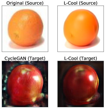
Figure 1: An example of orange2apple task. The baseline CycleGAN transfers an orange image to an apple image (left column). Our proposed L-Cool makes a slight change in the original orange image, which significantly improves the quality of the transferred apple image (right column): the green artifacts surrounding the apple were removed almost completely, and the texture and the color on the apple were improved, although slight blurry along the edges of the apple was introduced.

Table 1: Examples of French-English translation by XLM [18] and L-Cool. L-Cool makes the translation closer to the ground-truth.

Original sentence	Le prix du pétrole continue à baisser
	et se rapproche de 96 $ le baril
Ground-truth translation	Oil extends drop toward $ 96 a barrel
XLM [18] (baseline)	Oil price continues to drop
	and moves past $ 96 a barrel
L-Cool (Ours)	Oil price continues to drop
	and moves closer to $ 96 a barrel
Original sentence	" Au milieu de XXe siècle , on appelait cela une
	urgence psychiatrique " , a indiqué Drescher
Ground-truth translation	" Back in the middle of the 20th century , it was
	called a ’ psychiatric emergency ’ " said Drescher.
XLM [18] (baseline)	" In the late 20th century , we called
	this a psychiatric emergency , " Drescher said
L-Cool (Ours)	" In the middle of the 20th century , we called
	this a psychiatric emergency , " Drescher said .

In some DT applications, labeled samples, i.e., paired samples in the two domains, can be collected cheaply. For example, in the super-resolution, a paired low resolution image can be created by artificially blurring and down-sampling a high resolution image. However, in many other applications including image translation and language translation, collecting paired samples require significant human effort, and thus only a limited amount of paired data are available.

Unsupervised DT methods eliminate the necessity of paired data for supervision, and only require independent sets of training samples in both domains. In computer vision, CycleGAN, an extension of Generative Adversarial Networks (GAN) [30], showed its capability of unsupervised DT with impressive results in image translation tasks [31, 32, 33]. It learns the mappings between the two domains by matching the source training distribution transferred to the target domain and the target training distribution, under the cycle consistency constraint. Similar ideas were applied to natural language processing (NLP): Dual Learning [17, 34] and cross-lingual language models (XLM) [18], which are trained on unpaired monolingual data, achieved high performance in language translation.

Despite their remarkable successes, existing unsupervised DT methods are known to fail on a significant proportion of test samples [31, 35, 36]. In this paper, we hypothesize that some of the unsuccessful samples are at the fringe of the data distribution, i.e., they lie slightly off the data manifold, and therefore the DNN was not trained very well for translating those samples. This hypothesis leads to our proposal to bring fringe samples towards the high density data manifold, where the DNN is well-trained, by cooling down the test distribution. Specifically, our proposed method, called L-Cool, performs the Metropolis Adjusted Langevin Algorithm (MALA) to lower the temperature of test samples before applying the base DT method. The gradient of the log-probability, which MALA requires, is estimated by the denoising autoencoder (DAE) [37].

L-Cool is generic and can be used for enhancing any DT method. We demonstrate its effectiveness in image translation and language translation tasks, where L-Cool exhibits consistent performance gain. Figure 1 and Table 1 show a few intuitive exemplar results.

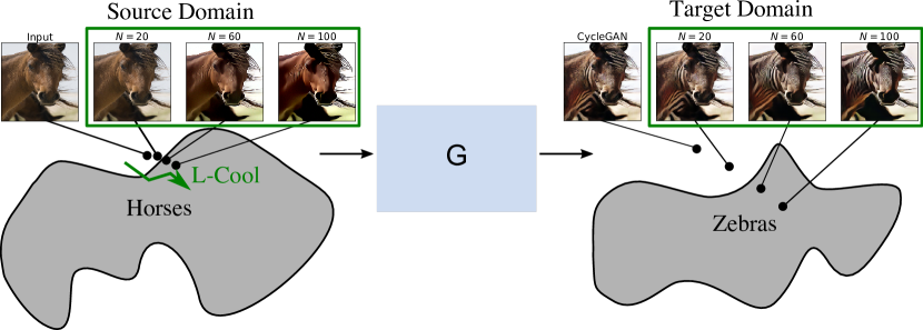
Figure 2: L-Cool drives the test sample in the source (horse) domain slightly towards the center of data manifold, which gives a significant impact on the translated sample in the target (zebra) domain.

This paper is an extension of our preliminary conference publication [38] with the following new contributions:

• Evaluation in Language translation (English $\leftrightarrow$ French and English $\leftrightarrow$ German) on the NewsCrawl dataset, which revealed quantitative performance gain by L-Cool in terms of the BLEU score [39].

• Comparison between the gradient estimators by DAE and by the cycle structure of CycleGAN. The latter was mainly used in the conference version.

• Analysis of hyperparameter dependence.

1.1 Related Work

1.1.1 Unsupervised Image Translation

CycleGAN [31] and its concurrent works [32, 33] have eliminated the necessity of supervision for image translation [22, 40] by using the loss inspired by GAN [30] along with the cycle-consistency loss. The consistency requirement forces translation to retain the contents of source images so that they can be translated back. [41] proposed a variant that shares the latent space between the two domains, which works as additional regularization for alleviating the highly ill-posed nature of unsupervised domain translation.

[42] and [43] tackled the general issue of unimodality in sample generation by splitting the latent space into two—a content space and a style space. The content space is shared between the two domains but the style space is unique to each domain. The style space is modeled with a Gaussian prior, which helps in generating diverse images at test time. [36, 44] showed that attention maps can boost the performance by making the model focus on relevant regions in the image. Despite a lot of new ideas proposed for improving the image translation performance, CycleGAN [31] is still considered to be the state-of-the-art in many transformation tasks.

1.1.2 Unsupervised Language Translation

Language translation has been tackled with DNNs with encoder-decoder architectures, where text in the source language is fed to the encoder and the decoder generates its translation in the target language [45]. Unsupervised language translation methods have enabled learning from a large pool of monolingual data [17, 46], which can be cheaply collected through the internet without any human labeling effort.

Transformers [34] with attention mechanisms have shown their excellent performance in unsupervised language translation, as well as many other NLP tasks including language modelling, understanding, and sentence classification. It was shown that generative pretraining strategies like Masked Language Modeling (which masks a portion of the words in the input sentence and forces the model to predict the masked words) is effective in making transformers better at language understanding [47, 48, 49, 50]. Back translation has also enhanced performance by being a source of data augmentation while maintaining the cycle consistency constraint [51, 19, 52]. Cross-lingual language models (XLM) [18] have shown state-of-the-art results in unsupervised language translation, outperforming GPT [47], BERT [49], and other previous methods [51, 53].

1.1.3 Temperature Control

Changing distributions by controlling the temperature has been used in Bayeasian learning and sample generation. [54] and [55] reported that sampling weights from its cooled posterior distribution improves the predictive performance in Bayesian learning. Higher quality images were generated from a reduced-temperature model in [56, 57, 58]. [57] used a tempered softmax for super resolution. In contrast to previous works that cool down estimated distributions (Bayes posterior or predictive distributions), our approach cools down the input test distribution to make fringe samples more typical for unsupervised domain translation.

2 Cooling Down Test Distributions

Our proposed method relies on two basic tools, the Metropolis-adjusted Langevin algorithm and a denoising autoencoder. After introducing those basic tools, we describe our method and its extensions.

2.1 Metropolis-adjusted Langevin Algorithm

The Metropolis-adjusted Langevin algorithm (MALA) is an efficient Markov chain Monte Carlo (MCMC) sampling method that uses the gradient of the energy (negative log-probability $E(\boldsymbol{x})=-\log p(\boldsymbol{x})$). Sampling is performed sequentially by

$$\boldsymbol{x}_{t+1}=\boldsymbol{x}_{t}+\alpha\boldsymbol{\nabla}_{\boldsymbol{x}}\log p(\boldsymbol{x}_{t})+\boldsymbol{\nu},$$ (1)

where $\alpha$ is the step size, and $\boldsymbol{\nu}$ is a random perturbation subject to $\mathcal{N}(\boldsymbol{0},\delta^{2}\boldsymbol{I}_{L})$. By appropriately controlling the step size $\alpha$ and the noise variance $\delta^{2}$, the sequence is known to converge to the distribution $p(\boldsymbol{x})$. [59] successfully generated high-resolution, realistic, and diverse artificial images by MALA.

2.2 Denoising Autoencoders (DAE)

A denoising autoencoder (DAE) [60, 61] is trained so that data samples contaminated with artificial noise are cleaned. Specifically, (an estimator) for the following reconstruction error is minimized:

$$L(\boldsymbol{r}) =\mathbb{E}_{p(\boldsymbol{x})p(\boldsymbol{\varepsilon})}\left[\|\boldsymbol{r}(\boldsymbol{x}+\boldsymbol{\varepsilon})-\boldsymbol{x}\|^{2}\right],$$ (2)

where $\mathbb{E}_{p}\left[\cdot\right]$ denotes the expectation over the distribution $p$, $\mathbb{R}^{L}\ni\boldsymbol{x}\sim p(\boldsymbol{x})$ is a data sample, and $\boldsymbol{\varepsilon}\sim p(\boldsymbol{\varepsilon})=\mathcal{N}_{L}(\boldsymbol{0},\sigma^{2}\boldsymbol{I})$ is artificial Gaussian noise with mean zero and variance $\sigma^{2}$. [37] discussed the relation between DAEs and contractive autoencoders, and proved the following useful property of DAEs:

Proposition 1

[37] Under the assumption that $\boldsymbol{r}(\boldsymbol{x})=\boldsymbol{x}+o(1)$, the minimizer of the DAE objective Eq.(2) satisfies

$$\boldsymbol{r}(\boldsymbol{x})-\boldsymbol{x}=\sigma^{2}\boldsymbol{\nabla}_{\boldsymbol{x}}\log p(\boldsymbol{x})+o(\sigma^{2}),$$ (3)

as $\sigma^{2}\to 0$.

Proposition 1 states that a DAE trained with a small $\sigma^{2}$ can be used to estimate the gradient of the log probability, i.e.,

$$\boldsymbol{\nabla}_{\boldsymbol{x}}\log p(\boldsymbol{x})\approx\widehat{\boldsymbol{g}}(\boldsymbol{x})\equiv\frac{\boldsymbol{r}(\boldsymbol{x})-\boldsymbol{x}}{\sigma^{2}}.$$ (4)

2.3 Langevin Cooling (L-Cool)

As discussed in Section 1, we hypothesize that domain translation (DT) methods can work poorly on test samples lying at the fringe of the data distribution. We therefore propose to drive such fringe samples towards the high density area, where the DNN is better trained. Specifically, we apply MALA Eq.(1) to each test sample with the step size $\alpha$ and the variance of the random perturbation satisfying the following inequality:

$$2\alpha>\delta^{2}.$$ (5)

If $2\alpha=\delta^{2}$, MALA can be seen as a discrete approximation to the (continuous) Langevin dynamics,

$$\frac{d\boldsymbol{x}}{dt} =\boldsymbol{\nabla}_{\boldsymbol{x}}\log p(\boldsymbol{x})+\sqrt{2}\frac{d\boldsymbol{W}}{dt},$$ (6)

where $\boldsymbol{W}$ is the Brownian motion. The dynamics Eq.(6) is known to converge to $p(\boldsymbol{x})$ as the equilibrium distribution [62, 63]. By setting the step size and the perturbation variance so that Inequality (5) holds, we can approximately draw samples from the distribution with lower temperature, as shown below.

By seeing the negative log probability as the energy $E(\boldsymbol{x})=-\log p(\boldsymbol{x})$, we can see $p(\boldsymbol{x})$ as the Boltzmann distribution with the inverse temperature equal to $\beta=1$:

$$p_{\beta}(\boldsymbol{x}) =\frac{1}{Z_{\beta}}\exp\left(-\beta E(\boldsymbol{x})\right),$$ (7)

where $Z_{\beta}=\int\exp\left(-\beta E(\boldsymbol{x})\right)d\boldsymbol{x}$ is the partition function. The following theorem holds:

Theorem 1

In the limit where $\alpha,\delta^{2}\to 0$ with their ratio $\alpha/\delta^{2}$ kept constant, the sequence of MALA Eq.(1) converges to $p_{\beta}(\boldsymbol{x})$ for

$$\beta=\frac{2\alpha}{\delta^{2}}.$$ (8)

(Proof) As $\alpha$ and $\delta^{2}$ go to $0$, MALA Eq.(1) converges to the following dynamics:

$$\frac{d\boldsymbol{x}}{dt} =\boldsymbol{\nabla}_{\boldsymbol{x}}\log p(\boldsymbol{x})+\frac{\delta}{\sqrt{\alpha}}\frac{d\boldsymbol{W}}{dt},$$

which is equivalent to

$$\frac{d\boldsymbol{x}}{dt} =\frac{2\alpha}{\delta^{2}}\boldsymbol{\nabla}_{\boldsymbol{x}}\log p(\boldsymbol{x})+\sqrt{2}\frac{d\boldsymbol{W}}{dt}.$$ (9)

Eq.(9) can be rewritten with the Boltzmann distribution Eq.(7) with the inverse temperature specified by Eq.(8):

$$\frac{d\boldsymbol{x}}{dt} =\boldsymbol{\nabla}_{\boldsymbol{x}}\log p_{\beta}(\boldsymbol{x})+\sqrt{2}\frac{d\boldsymbol{W}}{dt}.$$

Comparing it with Eq.(6), we find that this dynamics converges to the equilibrium distribution $p_{\beta}(\boldsymbol{x})$. $\Box$

Theorem 1 states that the ratio between $\alpha$ and $\delta^{2}$ effectively controls the temperature. Specifically, we can see MALA Eq.(1) as a discrete approximation to the Langevin dynamics converging to the distribution given by

$$p_{2\alpha/\delta^{2}}(\boldsymbol{x})=\frac{p^{2\alpha/\delta^{2}}(\boldsymbol{x})}{\int p^{2\alpha/\delta^{2}}(\boldsymbol{x})d\boldsymbol{x}},$$

of which the probability mass is more concentrated than $p(\boldsymbol{x})$ if Inequality (5) holds.

Our proposed Langevin cooling (L-Cool) strategy uses DAE for estimating the gradient, and applies MALA for $\beta>1$ to cool down test samples before DT is performed. As illustrated in Figure 2, this yields a small move of the test sample towards high density areas in the source domain. Since the DNN for DT is expected to be well trained on the high density areas, such a small move can result in a significant improvement of the translated image in the target domain, and thus enhances the DT performance. We show qualitative and quantitative performance gain by L-Cool in the subsequent sections.

2.4 Extensions

We can choose two options for L-Cool, depending on the application and computational resources.

2.4.1 Fringe Detection

We can apply fringe detection, in the same way as adversary detection [64]. Namely, assuming that the gradient of $\log p(\boldsymbol{x})$ is large at the fringe of the data distribution, we identify samples as fringe if

$$\left\|\boldsymbol{\nabla}_{\boldsymbol{x}}\log p(\boldsymbol{x})\right\|_{2}>\xi$$ (10)

for a threshold $\xi>0$, and apply MALA only to those samples. This prevents non-fringe samples already lying high density areas from being perturbed by Langevin dynamics.

2.4.2 Gradient Estimation by Cycle

Another option is to omit to train DAE, and estimate the gradient by a cycle structure that the DNN for DT already possesses. This idea follows the argument in [59], where MALA is successfully used to generate high-resolution, realistic, and diverse artificial images. The authors argued that DAE for estimating the gradient can be replaced with any cycle (autoencoding) structure in their application. In our image translation experiment, we use CycleGAN as the base method, and therefore, we can estimate the gradient by

$$\boldsymbol{\nabla}_{\boldsymbol{x}}\log p(\boldsymbol{x})\approx\widehat{\boldsymbol{g}}_{\mathrm{Cycle}}(\boldsymbol{x}) \equiv\gamma\left(\boldsymbol{F}(\boldsymbol{G}(\boldsymbol{x}))-\boldsymbol{x}\right)$$ (11)

for some $\gamma>0$, where $\boldsymbol{G}$ corresponds to the mapping of the CycleGAN from the source domain to the target domain and $\boldsymbol{F}$ to its inversion. We call this option L-Cool-Cycle, which eliminates the necessity of training DAE. However, one should use this option with care: we found that L-Cool-Cycle tends to exacerbate artifacts created by CycleGAN, which will be discussed in detail in Section 4.5.

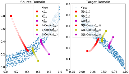
Figure 3: Toy data demonstration of L-Cool, which drives test samples, $x^{1}_{test},x^{2}_{test},x^{3}_{test}$, towards the data manifold in the source domain (left). This makes the translated samples $\boldsymbol{G}(x^{1}_{test}),\boldsymbol{G}(x^{2}_{test}),\boldsymbol{G}(x^{3}_{test})$ by CycleGAN more typical in the target domain (right).

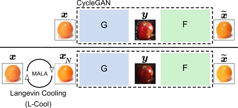
Figure 4: Schematics of (the plain) CycleGAN (top) and L-Cool (bottom). In CycleGAN, an encoder, $\boldsymbol{y}=\boldsymbol{G}(\boldsymbol{x})$, translates a source sample to a target sample, while a decoder, $\widetilde{\boldsymbol{x}}=\boldsymbol{F}(\boldsymbol{y})$, translates the target sample back to the source sample. In L-Cool, a source sample is cooled down by MALA, before being translated by CycleGAN.

3 Demonstration with Toy Data

We first show the basic behavior of L-Cool on toy data. We generated $1,000$ training samples each in the source and the target domains by

$$\boldsymbol{x} =(t,0.75\times t^{2}+\epsilon), \boldsymbol{x}^{\prime} =(t^{\prime},0.4\times t^{\prime}+\epsilon^{\prime}),$$

respectively, where $t,t^{\prime}\sim\mathrm{Uniform}(0,1)$, $\epsilon\sim\mathrm{Uniform}(0,0.2)$, and $\epsilon^{\prime}\sim\mathrm{Uniform}(0,0.1)$. Then, a CycleGAN [31] with two-layer feed forward networks, $\boldsymbol{G}(\boldsymbol{x})\to\widehat{\boldsymbol{x}}^{\prime}$ and $\boldsymbol{F}(\boldsymbol{x}^{\prime})\to\widehat{\boldsymbol{x}}$, were trained to learn the forward and the inverse mappings between the two domains. A DAE having the same architecture as $\boldsymbol{G}$ with two-layer feed forward network was also trained on the samples in the source domain.

Blue dots in Figure 3 show training samples, from which we can see the high density areas both in the source (right) and the target (left) domains. Now we feed three off-manifold test samples $x^{1}_{test},x^{2}_{test},x^{3}_{test}$, shown as red, yellow, and magenta squares in the left graph, to the forward (source to target) translator $\boldsymbol{G}$. As expected, the translated samples $\boldsymbol{G}(x^{1}_{test}),\boldsymbol{G}(x^{2}_{test}),\boldsymbol{G}(x^{3}_{test})$, shown as red, yellow, and magenta squares in the right graph, are not in the high density area (not typical target samples), because $\boldsymbol{G}$ was not trained for those off-manifold samples. As shown as trails of circles, L-Cool drives the off-manifold samples into the data manifold in the source domain, which also drives the translated samples into the data manifold in the target domain. This way, L-Cool helps CycleGAN generate typical samples in the target domain by making source samples more typical.

4 Image Translation Experiments

Next, we demonstrate the performance of L-Cool in several image translation tasks. We use CycleGAN as the base translation method, and L-Cool is performed in the source image space before translation (Figure 4).

4.1 Translation Tasks and Model Architectures

We used pretrained CycleGAN models, along with the training and the test datasets, publicly available in the official Github repository of CycleGAN [31]. Experiments were conducted on the following tasks.

horse2zebra

Translation from horse images to zebra images and vice versa. The training set consists of $1067$ horse images and $1334$ zebra images, subsampled from ImageNet. Dividing the test set, we prepared $60$ and $70$ validation images and $60$ and $70$ test images for horse and zebra, respectively.

apple2orange

Translation from apple images to orange images and vice versa. The training set consists of $995$ apple images and $1019$ orange images, subsampled from ImageNet. Dividing the test set, we prepared $133$ and $133$ validation images and $133$ and $133$ test images for apple and orange, respectively.

sat2map

Translation from satellite images to map images. The training set consists of $1096$ satellite images and $1096$ map images, subsampled from Google Maps. $1098$ and $1098$ images each are provided for test. Dividing the test set, we prepared $250$ validation images and $848$ test images. Although CycleGAN was pretrained in the unsupervised setting, the dataset is actually paired, i.e., the ground truth map image for each satellite image is available, which allows quantitative evaluation.

For the first two tasks, we also conducted experiments on the inverse tasks, i.e., zebra2horse and orange2apple. The validation images were used for hyperparameter tuning for L-Cool (see Section 4.4).

The CycleGAN model consists of a forward mapping $\boldsymbol{G}$ and a reverse mapping $\boldsymbol{F}$. Both $\boldsymbol{G}$ and $\boldsymbol{F}$ have the same architecture including $2$ downsampling layers followed by $9$ resnet generator blocks and $2$ upsampling layers. Each resnet generator block consists of convolution, batch normalization [65] and ReLU layers with residual connections added between every block.

For DAE, we adapted a Tiramisu model [66] consisting $67$ layers in total. The PyTorch [67] code for Tiramisu was obtained from a publicly available GitHub reporsitory. The Tiramisu consists of $5$ downsampling layers followed by a bottleneck layer and $5$ upsampling layers. Each downsampling as well as upsampling layer consists of dense blocks with a growth rate of $16$. Each dense block consists of batch normalization [65], ReLU, and convolution layers with dense connections [68]. We trained the DAE on the training images in the source domain for $200$ epochs by the Adam optimizer with the learning rate set to $0.0002$.

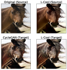
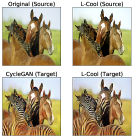
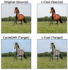
(a) horse2zebra: The contrast of stripes are increased (left and middle) and artifacts around the zebra are reduced (right).

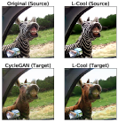
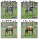
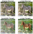
(b) zebra2horse: The color of the horse body is improved.

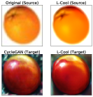
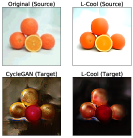
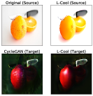
(c) orange2apple: The texture and the color of apples are improved, and artifacts in the background are reduced.

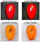
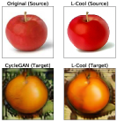
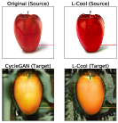
(d) apple2orange: The color of oranges is improved.

Figure 5: Example results of image translation tasks. Three examples for each task are shown, and each example shows the original test image (top left) and the image after L-Cool is applied (top right) in the source domain, and their translated images (bottom left and right) in the target domain.

4.2 Qualitative Evaluation

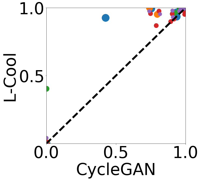
(a) %fringes: $20$

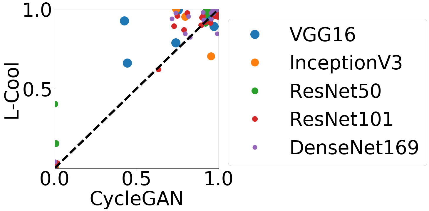
(b) %fringes: $40$

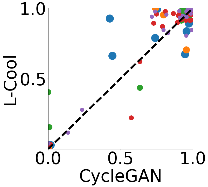
(c) %fringes: $60$

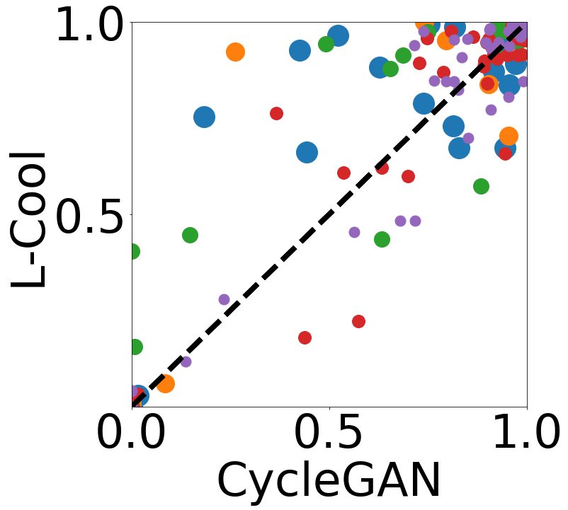
(d) %fringes: $80$

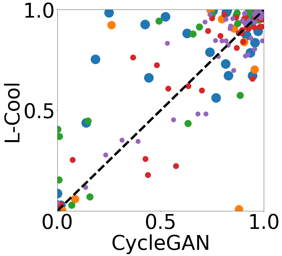
(e) %fringes: $100$

Figure 6: Likeness to zebra images evaluated by the probability output $p(\boldsymbol{y}=\textrm{zebra}|\boldsymbol{x})$ of pretrained classifiers for the translated images by CycleGAN (horizontal axis) and by L-Cool (vertical axis). Each panel plots the fringe samples identified by the fringe detector for different proportions. We can see that, consistently for all classifiers (shown in different colors), points tend to be above the equal-likeness dashed line, implying improvement by L-Cool.

Table 2: Average likeness to zebra images over the fringe samples and the classifiers (shown in the legend in Figure 6). For each row, the methods that are not significantly outperformed by the other are bold-faced, according to the Wilcoxon signed rank test for $p=0.05$.

% fringes	CycleGAN	L-Cool
20 40 60 80 100	0.6910 0.7872 0.8023 0.8138 0.8022	0.7385 0.8145 0.8167 0.8331 0.8211

Figure 5 shows some example results of horse2zebra, zebra2horse, apple2orange, and orange2apple tasks. We see that L-Cool moves original source images more typical (in terms of color and smoothness), which results in improved translated images, e.g., more stripes in (a) horse2zebra, more brown color in the horse body in (b) zebra2horse, better texture and color in (c) apple2orange and (d) orange2apple, and removal of artifacts in general.

4.3 Quantitative Evaluation

In order to confirm that L-Cool generally improves the image translation performance, we conducted two experiments that quantitatively evaluate the performance.

4.3.1 Likeness Evaluation by Pretrained Classifiers

Focusing on horse2zebra, we evaluated the likeness of the translated images to zebra images by using state-of-the-art classifiers, including VGG16 [69], InceptionV3 [70], Resnet50 [71], Resnet101 [72], and DenseNet169 [68] pretrained on the ImageNet dataset [73]. Specifically, we evaluated and compared the probability outputs (i.e., after soft-max) of the classifiers for the translated images by plain CycleGAN and those by L-Cool. We applied fringe detection, Eq.(10), with the threshold $\xi$ adjusted so that specified proportions (20%, 40%, 60%, 80%, and 100%) of the test samples are identified as fringe. Note that $100\%$ fringe samples correspond to L-Cool without fringe detection (all test samples are cooled down by MALA).

Figure 6 shows scatter plots of likeness to zebra images, i.e., the probability $p(\boldsymbol{y}=\textrm{zebra}|\boldsymbol{x})$ evaluated by pretrained classifiers. The five panels respectively plot the $20,40,60$, $80$ and $100\%$ fringe samples. In each plot, the horizontal axis corresponds to the likeness of the transferred images by CycleGAN, while the vertical axis corresponds to the likeness of the transferred images by L-Cool. The dashed line indicates the equal-probability, i.e., the points above the dashed line imply the improvement by L-Cool.

We observe that all classifiers tend to give higher probability to the images translated after L-Cool is applied. We emphasize that L-Cool uses no information on the target domain—DAE is trained purely on the samples in the source domain, and MALA drives samples towards high density areas in the source domain, independently from the translation task. The hyperparameters for the Langevin dynamics were set to $\alpha=0.005$, $\beta^{-1}=0.001$ and $N=40$, which were found optimal on the validation set (see Section 4.4). Table 2 shows the average likeness over the fringe samples and the five classifiers.

We observe in Table 2 that, for smaller proportions of fringe samples (first column), the performance of the plain CycleGAN (second column) is worse, and the performance gain, i.e., the differences between L-Cool (third column) and CycleGAN, is larger. These observations empirically support our hypothesis that CycleGAN does not perform well on fringe samples, and cooling down those samples can improve the translation performance.

4.3.2 Evaluation on Paired-data

As mentioned in Section 5.1, sat2map dataset consists of pairs of satellite images and the corresponding map images, and therefore allows us to directly evaluate image translation performance. We applied the pretrained CycleGAN to the test satellite images with and without L-Cool, and compared the transferred map images with the corresponding ground-truth map images. Following the evaluation procedure in [41], we counted pixels as correct if the color mismatch (i.e., the Euclidean distance between the transferred map and the ground-truth map in the RGB color space) is below 16.

Table 3: Average pixel-wise accuracy in the sat2map task. For each row, the methods that are not significantly outperformed by the other are bold-faced, according to the Wilcoxon signed rank test for $p=0.05$.

%fringes	CycleGAN	L-Cool
20	61.83	62.76
40	65.95	66.37
60	66.37	67.54
80	68.56	68.76
100	68.83	69.05

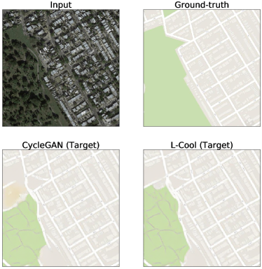
Figure 7: An example of sat2map image translation result. L-Cool result (bottom right) is closer to the ground truth (top right) than the plain CycleGAN (bottom left).

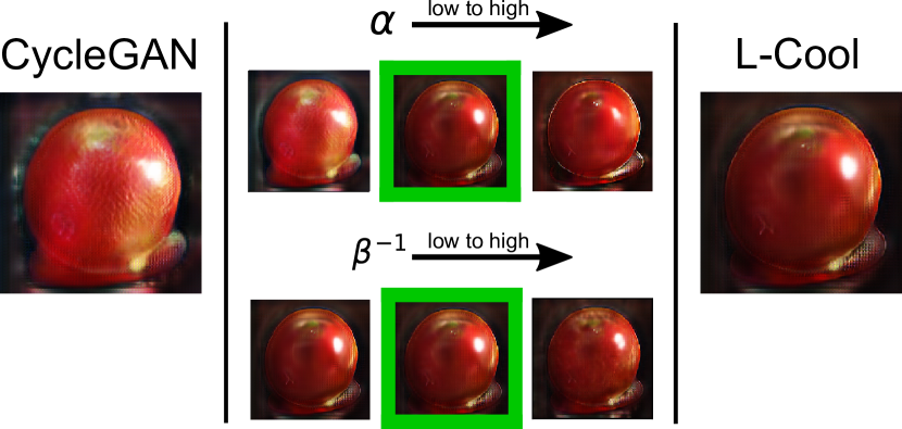
Figure 8: Translated images by L-Cool with different hyperparameter settings. We found that the setting $\beta^{-1}=0.001$, $\alpha=0.005$, and $N=100$ (marked with a green bounding box) best removes artifacts and increases the target domain attributes.

Table 3 shows the average pixel-wise accuracy, where we observed a similar tendency to the likeness evaluation in Section 4.3.1: for smaller proportions of fringe samples, the translation performance of the plain CycleGAN is worse, and the performance gain by L-Cool is larger. Figure 7 shows an exemplar case where L-Cool improves translation performance.

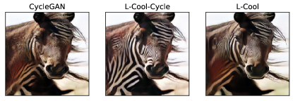
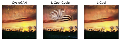
Figure 9: Translated images by CycleGAN (left column), L-Cool-Cycle (middle column), and L-Cool (right column). L-Cool-Cycle tends to enhance target domain attributes more than L-Cool (top row), but also tends to exacerbate artifacts (bottom row).

4.4 Hyperparameter Setting

L-Cool has several hyperparameters. For DAE traning, we set the training noise to $\sigma=0.3$ for all tasks, which approximately follows the recommendation ($10\%$ of the mean pixel values) in [59]. We visually inspected the performance dependence on the remaining hyperparameters, i.e., temperature $\beta^{-1}$, step size $\alpha$, and the number of steps $N$. Roughly speaking, the product of $\alpha$ and $N$ determines how far the resulting image can reach from the original point, and similar results are obtained if $\alpha\cdot N$ has similar values, as long as the step size $\alpha$ is sufficiently small.

Figure 8 shows exemplarily translated images in the orange2apple task, where the dependence on the temperature $\beta^{-1}$ and the step size $\alpha$ is shown for the number of steps fixed to $N=100$. We observed that, as the step size $\alpha$ increases, the translated image gets more attributes—increased red color on the apple—of the target domain, and artifacts are reduced. However, if $\alpha$ is too large, the image gets blurred. We also observed that too high temperature $\beta^{-1}$ gives noisy result. The visually best result was obtained when $\beta^{-1}=0.001$, $\alpha=0.005$ and $N=100$ (marked with a green box and plotted on the right most in Figure 8). Similar tendency was observed in other test samples and other tasks.

For quantitative evaluations in Section 4.3, we optimized the hyperparameters on the validation set. The reported results were obtained with the hyperparameters searched over $\beta^{-1}=0.0001,0.001,0.005,0.01$, $\alpha=0.001,0.005,0.01$, and $N=20,40,60,80,100$.

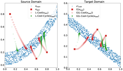
Figure 10: The same toy data demonstration as Figure 3, comparing L-Cool (red) and L-Cool-Cycle (green). In contrast with L-Cool, L-Cool-Cycle does not move samples directly towards the high density region in the source domain, implying that the cycle gradient estimator is not a very good substitution for DAE gradient estimator.

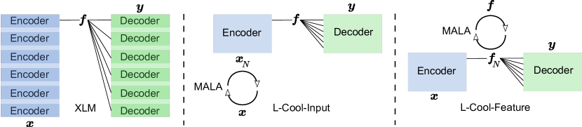
Figure 11: Schematics of XLM (left), L-Cool-Input (middle), and L-Cool-Feature (right). L-Cool-Input performs MALA in the input space, while L-Cool-Feature performs MALA in the feature (code) space between the encoder and the decoder.

4.5 Investigation on the L-Cool-Cycle

L-Cool requires a trained DAE for gradient estimation. However, a variant, introduced in Section 2.4.2 as an option called L-Cool-Cycle, eliminates the necessity of DAE training, and estimate the gradient by using the autoencoding structure of CycleGAN. This option empirically showed good performance in image generation [59], as well as in our preliminary experiments in image translation [38].

However, further investigation revealed a drawback of this variant: although L-Cool-Cycle tends to enhance attributes of the target domain images, it also tends to exacerbate artifacts. Figure 9 shows this tendency: L-Cool-Cycle increases the contrast of stripes on the zebra body in the horse2zebra task (top row), while it aggravates the stripe artifacts on the sky (bottom row). In the latter case, we see that L-Cool (with DAE) rather suppresses the artifacts.

Suboptimality of L-Cool-Cycle can already be seen in the toy data experiment. Figure 10 shows the same demonstration as in Figure 3, and compares trails by L-Cool and L-Cool-Cycle. We see that L-Cool (red) drives the off-manifold samples directly towards the data manifold, while L-Cool-Cycle (green) does not always do so. This implies that the cycle estimator Eq.(11) is not a very good gradient estimator.

In summary, although L-Cool-Cycle is an option when training DAE is hard or time-consuming, it should be used in care—resulting samples should be checked by human.

5 Language Translation Experiments

In this section, we demonstrate the performance of our proposed L-Cool in language translation tasks with Cross-lingual Language Model (XLM) [51, 18]—a state-of-the-art method for unsupervised language translation—as the base method.

5.1 Translation Tasks and Model Architectures

We conducted experiments on four language translation tasks, EN-FR, FR-EN, EN-DE, and DE-EN, based on NewsCrawl dataset under the default setting defined in the GitHub repository page: for each pair of languages, we used the first $5$M sentences for training, $3000$ sentences for validation, and $3000$ sentences for test.

The main idea of XLM is to share sub-word vocabulary between the source and the target languages created through the Byte Pair Encoding (BPE). Masked Language Modeling (MLM) is performed as pretraining, similarly to BERT [49]. $15\%$ of the BPE from the text stream is masked $80\%$ of the time, by a random token $10\%$ of the time and they are kept unchanged $10\%$ of the time. The encoder is pretrained with the MLM objective, whose weights are then used as initialization for both the encoder and the decoder. This pretraining strategy was shown to give the best results [18].

The transformer consists of $6$ encoders and $6$ decoders. The architectures of encoders and decoders are similar, and each consists of a multi-head attention layer followed by layer normalization [74], $2$ fully connected layers with GELU activations [75] and another layer normalization. While the first fully connected layer projects the input with a dimensionality of $1024$ to a latent dimension of $4096$, the second fully connected layer projects it back to $1024$. Each encoder and decoder layer also consists of a residual connection. For XLM implementation, we use the code publicly available at the GitHub page. We train the model by using the ADAM optimizer along with linear warm-up and linear learning rates. We warm start with the model weights obtained after the MLM stage, and further train the weights on the training sentences.

We tested two variants of L-Cool (see Figure 11).

L-Cool-Input:

MALA is performed in the input word embedding space (the position embeddings are unaffected).

L-Cool-Feature:

MALA is performed in the intermediate feature (code) space.

DAE with the same architecture as the encoder of the transformer was trained in the corresponding space on the training sentences of NewsCrawl. Hyperparameters were tuned on the validation sentences (see Section 5.3).

Table 4: BLEU scores in language translation tasks.

	EN-FR	FR-EN	EN-DE	DE-EN
XLM (Baseline)	33.46	31.62	25.51	31.11
L-Cool-Input	31.59	31.90	25.66	30.93
L-Cool-Feature	33.91	31.93	25.73	31.17

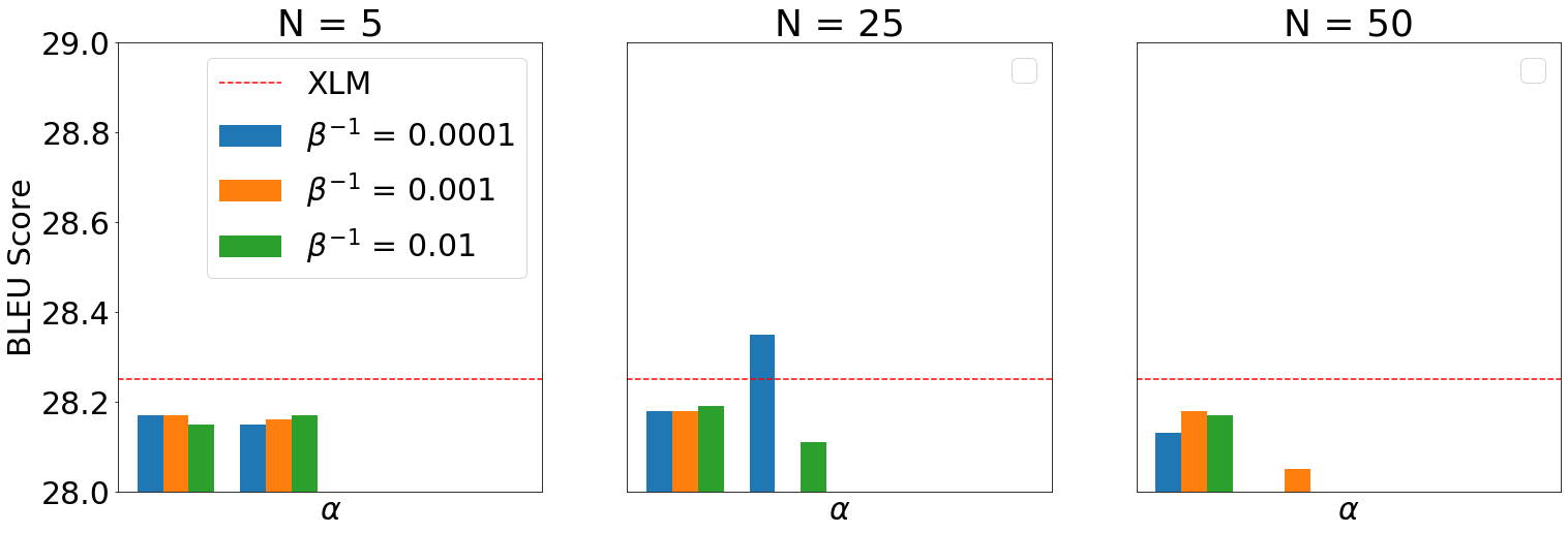
(a) L-Cool-Input

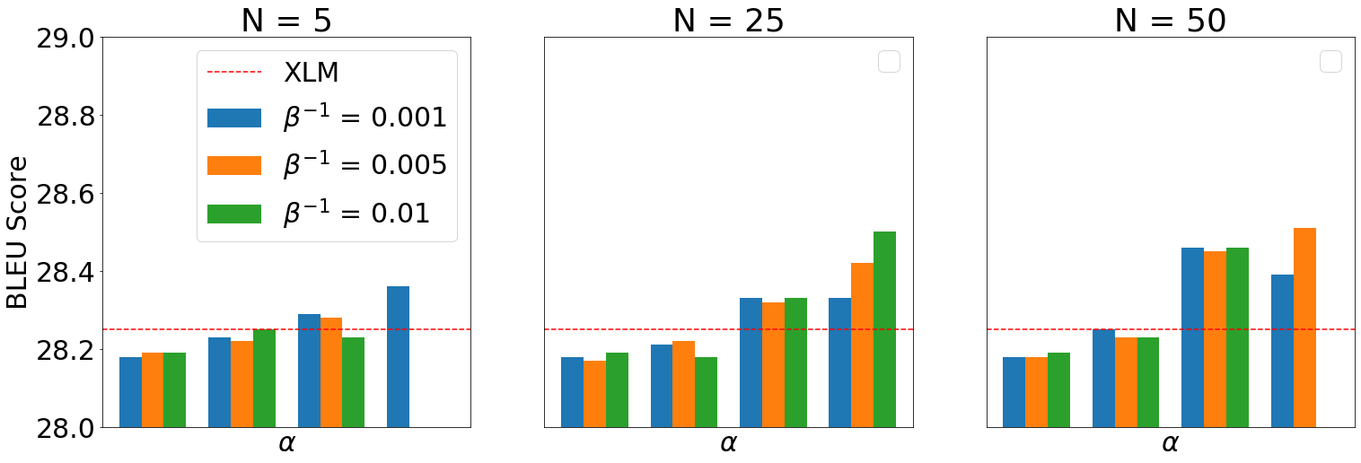
(b) L-Cool-Feature

Figure 12: Language translation performance (BLEU score) dependence on hyperparameters in the EN-FR task with L-Cool-Input (left) and L-Cool-Feature (right). The dashed line in each graph indicates the baseline performance by plain XLM.

5.2 Quantitative Evaluation

Table 4 shows the BLEU scores [39] by plain XLM, L-Cool-Input, and L-Cool-Feature, where we see consistent performance gain over all tasks by L-Cool-Feature. L-Cool-Input does not improves the performance, and even degrades in some tasks. We conjecture that this is because of the discrete nature of the input space—the input is the word embedding that depends only on discrete occurrences of words, and therefore, a single step of MALA to any direction can bring the sample to a point where the base transformer is less trained than the original point.

5.3 Hyperparameter Setting

Similarly to Section 4.4, we set the DAE training noise to $\sigma^{2}=0.1$ for L-Cool-Input and $\sigma^{2}=1.0$ for L-Cool-Feature, which approximately follow the recommendation in [59]. The remaining hyperparameters, i.e., temperature $\beta^{-1}$, step size $\alpha$, and the number of steps $N$, were tuned by maximizing the BLEU score on the validation sentences. The search ranges were $\beta^{-1}=0.0001,0.0005,0.001,0.005,0.01$, $\alpha=0.001,0.005,0.01$, $0.05$, $0.1$ and $N=5,25,50$, respectively.

Figure 12 shows performance dependence on the hyperparmaeters for L-Cool-Input (left) and L-Cool-Feature (right) in the EN-FR translation task, where the best performance was obtained when $\beta^{-1}=10^{-4},\alpha=10^{-5},N=25$ for L-Cool-Input, and when $\beta^{-1}=10^{-3},\alpha=10^{-2},N=25$ for L-Cool-Feature.

6 Computation Time

L-Cool requires additional computation cost both in training and test. Training the DAE can typically be done much faster than training the base DNN for the domain translation. In our experiment for the horse2zebra image translation task, training the DAE took $\sim 12800$ seconds or $3.55$ hours, while training the CycleGAN typically takes $\sim 42320$ seconds or $11.75$ hours (we did not train it because we used a pretrained network provided by the authors of CycleGAN). Note that this additional training is not necessary for L-Cool-Cycle, which substitutes the cycle structure of the base DNN for gradient estimation. In the test time, L-Cool requires $10$ to $100$ times more computation time, depending on the number of MALA steps. This is because DAE should have a similar structure and complexity to the base DNN. In our image translation experiment, L-Cool and CycleGAN took $\sim 5.3$ seconds and $\sim 0.5$ seconds per test image, respectively, while in the language translation experiment, L-Cool and XLM took $\sim 0.047$ seconds and $\sim 0.013$ per test sentence, respectively.

7 Conclusion

Developing unsupervised, as well as self-supervised, learning methods, is one of the recent hot topics in the machine learning community for computer vision [76, 77, 78, 79, 80] and natural language processing [49, 81, 82, 48, 83]. It is challenging but highly attractive since eliminating the necessity of labeled data may enable us to keep improving learning machines from data stream automatically without any human intervention. The successes of deep learning in the unsupervised domain translation (DT) was a milestone in this exciting research area.

Our work contributes to this area with a simple idea. Namely, Langevin Cooling (L-Cool) performs Metropolis Adjusted Langevin Algorithm (MALA) to test samples in the source domain, and drives them towards high density manifold, where the base deep neural network is well-trained. Our qualitative and quantitative evaluations showed improvements by L-Cool in image and language translation tasks, supporting our hypothesis that a proportion of test samples are failed to be translated because they lie at the fringe of data distribution, and therefore can be improved by L-Cool.

L-Cool is generic and can be used to improve any DT method. Future work is therefore to apply L-Cool to other base DT methods and other DT tasks. We will also try to improve the gradient estimator for L-Cool by using other types of generative models such as normalizing flows [84]. Explanation methods, such as layer-wise relevance propagation (e.g. [85, 86, 87]), might help identify the reasons for successes and failures [88] of DT, suggesting possible ways to improve the performance.

8 Acknowledgements

The authors acknowledge financial support by the German Ministry for Education and Research (BMBF) for the Berlin Center for Machine Learning (01IS18037A), Berlin Big Data Center (01IS18025A) and under the Grants 01IS14013A-E, 01GQ1115 and 01GQ0850; Deutsche Forschungsgemeinschaft (DFG) under Grant Math+, EXC 2046/1,Project ID 390685689 and by the Technology Promotion(IITP) grant funded by the Korea government (No. 2017-0-00451). Correspondence to WS, SN and KRM.

References

- [1] R. Biswas, M. K. Sen, V. Das, and T. Mukerji, “Prestack and poststack inversion using a physics-guided convolutional neural network,” Interpretation, vol. 7, no. 3, pp. SE161–SE174, 2019.
- [2] J. Gilmer, S. S. Schoenholz, P. F. Riley, O. Vinyals, and G. E. Dahl, “Neural message passing for quantum chemistry,” in International Conference on Machine Learning, 2017, pp. 1263–1272.
- [3] K. Schütt, P.-J. Kindermans, H. E. S. Felix, S. Chmiela, A. Tkatchenko, and K.-R. Müller, “Schnet: A continuous-filter convolutional neural network for modeling quantum interactions,” in Advances in neural information processing systems, 2017, pp. 991–1001.
- [4] K. Schütt, M. Gastegger, A. Tkatchenko, K.-R. Müller, and R. J. Maurer, “Unifying machine learning and quantum chemistry with a deep neural network for molecular wavefunctions,” Nature communications, vol. 10, no. 1, pp. 1–10, 2019.
- [5] G. Zhang, Z. Wang, and Y. Chen, “Deep learning for seismic lithology prediction,” Geophysical Journal International, vol. 215, no. 2, pp. 1368–1387, 2018.
- [6] J. Schmidt, M. R. Marques, S. Botti, and M. A. Marques, “Recent advances and applications of machine learning in solid-state materials science,” npj Computational Materials, vol. 5, no. 1, pp. 1–36, 2019.
- [7] S. Arridge, P. Maass, O. Öktem, and C.-B. Schönlieb, “Solving inverse problems using data-driven models,” Acta Numerica, vol. 28, pp. 1–174, 2019.
- [8] T. A. Bubba, G. Kutyniok, M. Lassas, M. März, W. Samek, S. Siltanen, and V. Srinivasan, “Learning the invisible: A hybrid deep learning-shearlet framework for limited angle computed tomography,” Inverse Problems, vol. 35, no. 6, p. 064002, 2019.
- [9] F. Codevilla, M. Miiller, A. López, V. Koltun, and A. Dosovitskiy, “End-to-end driving via conditional imitation learning,” in 2018 IEEE International Conference on Robotics and Automation (ICRA). IEEE, 2018, pp. 1–9.
- [10] A. Dosovitskiy, G. Ros, F. Codevilla, A. Lopez, and V. Koltun, “Carla: An open urban driving simulator,” in Conference on Robot Learning, 2017, pp. 1–16.
- [11] Unknown, “Developers, start your engines,” 2020. [Online]. Available: https://aws.amazon.com/deepracer/
- [12] D. Gray, “Introducing voyage deepdrive,” 2019. [Online]. Available: https://news.voyage.auto/introducing-voyage-deepdrive-69b3cf0f0be6
- [13] B. McMahan and D. Ramage, “Federated learning: Collaborative machine learning without centralized training data,” 2017. [Online]. Available: https://ai.googleblog.com/2017/04/federated-learning-collaborative.html-g/
- [14] Y. Wu, M. Schuster, Z. Chen, Q. V. Le, M. Norouzi, W. Macherey, M. Krikun, Y. Cao, Q. Gao, K. Macherey et al., “Google’s neural machine translation system: Bridging the gap between human and machine translation,” arXiv preprint arXiv:1609.08144, 2016.
- [15] Unknown, “Game intelligence,” 2020. [Online]. Available: https://www.microsoft.com/en-us/research/theme/game-intelligence/
- [16] J. Johnson, A. Alahi, and L. Fei-Fei, “Perceptual losses for real-time style transfer and super-resolution,” in European conference on computer vision. Springer, 2016, pp. 694–711.
- [17] D. He, Y. Xia, T. Qin, L. Wang, N. Yu, T.-Y. Liu, and W.-Y. Ma, “Dual learning for machine translation,” in Advances in neural information processing systems, 2016, pp. 820–828.
- [18] A. Conneau and G. Lample, “Cross-lingual language model pretraining,” in Advances in Neural Information Processing Systems, 2019, pp. 7059–7069.
- [19] S. Edunov, M. Ott, M. Auli, and D. Grangier, “Understanding back-translation at scale,” Proceedings of the 2018 Conference on Empirical Methods in Natural Language Processing, pp. 489–500, 2018.
- [20] L. A. Gatys, A. S. Ecker, and M. Bethge, “A neural algorithm of artistic style,” arXiv preprint arXiv:1508.06576, 2015.
- [21] C. Dong, C. C. Loy, K. He, and X. Tang, “Image super-resolution using deep convolutional networks,” IEEE transactions on pattern analysis and machine intelligence, vol. 38, no. 2, pp. 295–307, 2015.
- [22] P. Isola, J.-Y. Zhu, T. Zhou, and A. A. Efros, “Image-to-image translation with conditional adversarial networks,” in Proceedings of the IEEE conference on computer vision and pattern recognition, 2017, pp. 1125–1134.
- [23] D. Ulyanov, A. Vedaldi, and V. Lempitsky, “Deep image prior,” in Proceedings of the IEEE Conference on Computer Vision and Pattern Recognition, 2018, pp. 9446–9454.
- [24] S. Reed, Z. Akata, X. Yan, L. Logeswaran, B. Schiele, and H. Lee, “Generative adversarial text to image synthesis,” arXiv preprint arXiv:1605.05396, 2016.
- [25] H. Zhang, T. Xu, H. Li, S. Zhang, X. Wang, X. Huang, and D. N. Metaxas, “Stackgan: Text to photo-realistic image synthesis with stacked generative adversarial networks,” in Proceedings of the IEEE international conference on computer vision, 2017, pp. 5907–5915.
- [26] V. Sandfort, K. Yan, P. J. Pickhardt, and R. M. Summers, “Data augmentation using generative adversarial networks (cyclegan) to improve generalizability in ct segmentation tasks,” Scientific reports, vol. 9, no. 1, pp. 1–9, 2019.
- [27] E. Wu, K. Wu, D. Cox, and W. Lotter, “Conditional infilling gans for data augmentation in mammogram classification,” in Image Analysis for Moving Organ, Breast, and Thoracic Images. Springer, 2018, pp. 98–106.
- [28] M. Frid-Adar, E. Klang, M. Amitai, J. Goldberger, and H. Greenspan, “Synthetic data augmentation using gan for improved liver lesion classification,” in 2018 IEEE 15th international symposium on biomedical imaging (ISBI 2018). IEEE, 2018, pp. 289–293.
- [29] C. Bowles, L. Chen, R. Guerrero, P. Bentley, R. Gunn, A. Hammers, D. A. Dickie, M. V. Hernández, J. Wardlaw, and D. Rueckert, “Gan augmentation: Augmenting training data using generative adversarial networks,” arXiv preprint arXiv:1810.10863, 2018.
- [30] I. Goodfellow, J. Pouget-Abadie, M. Mirza, B. Xu, D. Warde-Farley, S. Ozair, A. Courville, and Y. Bengio, “Generative adversarial nets,” in Advances in neural information processing systems, 2014, pp. 2672–2680.
- [31] J.-Y. Zhu, T. Park, P. Isola, and A. A. Efros, “Unpaired image-to-image translation using cycle-consistent adversarial networks,” in Proceedings of the IEEE international conference on computer vision, 2017, pp. 2223–2232.
- [32] T. Kim, M. Cha, H. Kim, J. K. Lee, and J. Kim, “Learning to discover cross-domain relations with generative adversarial networks,” in Proceedings of the 34th International Conference on Machine Learning-Volume 70. JMLR. org, 2017, pp. 1857–1865.
- [33] Z. Yi, H. Zhang, P. Tan, and M. Gong, “Dualgan: Unsupervised dual learning for image-to-image translation,” in Proceedings of the IEEE international conference on computer vision, 2017, pp. 2849–2857.
- [34] A. Vaswani, N. Shazeer, N. Parmar, J. Uszkoreit, L. Jones, A. N. Gomez, Ł. Kaiser, and I. Polosukhin, “Attention is all you need,” in Advances in neural information processing systems, 2017, pp. 5998–6008.
- [35] “Cyclegan,” https://github.com/junyanz/CycleGAN#failure-cases.
- [36] Y. A. Mejjati, C. Richardt, J. Tompkin, D. Cosker, and K. I. Kim, “Unsupervised attention-guided image-to-image translation,” in Advances in Neural Information Processing Systems, 2018, pp. 3693–3703.
- [37] G. Alain and Y. Bengio, “What regularized auto-encoders learn from the data-generating distribution,” The Journal of Machine Learning Research, vol. 15, no. 1, pp. 3563–3593, 2014.
- [38] V. Srinivasan, K.-R. Müller, W. Samek, and S. Nakajima, “Benign examples: Imperceptible changes can enhance image translation performance,” in Proceedings of the Thirty-Fourth AAAI Conference on Artificial Intelligence, 2020.
- [39] K. Papineni, S. Roukos, T. Ward, and W.-J. Zhu, “Bleu: a method for automatic evaluation of machine translation,” in Proceedings of the 40th annual meeting on association for computational linguistics. Association for Computational Linguistics, 2002, pp. 311–318.
- [40] T.-C. Wang, M.-Y. Liu, J.-Y. Zhu, A. Tao, J. Kautz, and B. Catanzaro, “High-resolution image synthesis and semantic manipulation with conditional gans,” in Proceedings of the IEEE conference on computer vision and pattern recognition, 2018, pp. 8798–8807.
- [41] M.-Y. Liu, T. Breuel, and J. Kautz, “Unsupervised image-to-image translation networks,” in Advances in neural information processing systems, 2017, pp. 700–708.
- [42] X. Huang, M.-Y. Liu, S. Belongie, and J. Kautz, “Multimodal unsupervised image-to-image translation,” in Proceedings of the European Conference on Computer Vision (ECCV), 2018, pp. 172–189.
- [43] H.-Y. Lee, H.-Y. Tseng, J.-B. Huang, M. Singh, and M.-H. Yang, “Diverse image-to-image translation via disentangled representations,” in Proceedings of the European Conference on Computer Vision (ECCV), 2018, pp. 35–51.
- [44] J. Kim, M. Kim, H. Kang, and K. Lee, “U-GAT-IT: unsupervised generative attentional networks with adaptive layer-instance normalization for image-to-image translation,” CoRR, vol. abs/1907.10830, 2019. [Online]. Available: http://arxiv.org/abs/1907.10830
- [45] D. Bahdanau, K. Cho, and Y. Bengio, “Neural machine translation by jointly learning to align and translate,” arXiv preprint arXiv:1409.0473, 2014.
- [46] M. Artetxe, G. Labaka, E. Agirre, and K. Cho, “Unsupervised neural machine translation,” arXiv preprint arXiv:1710.11041, 2017.
- [47] A. Radford, K. Narasimhan, T. Salimans, and I. Sutskever, “Improving language understanding by generative pre-training,” 2018.
- [48] A. Radford, J. Wu, R. Child, D. Luan, D. Amodei, and I. Sutskever, “Language models are unsupervised multitask learners,” OpenAI Blog, vol. 1, no. 8, p. 9, 2019.
- [49] J. Devlin, M.-W. Chang, K. Lee, and K. Toutanova, “Bert: Pre-training of deep bidirectional transformers for language understanding,” in Proceedings of the 2019 Conference of the North American Chapter of the Association for Computational Linguistics: Human Language Technologies, Volume 1 (Long and Short Papers), 2019, pp. 4171–4186.
- [50] “Bart: Denoising sequence-to-sequence pre-training for natural language generation, translation, and comprehension,” arXiv preprint arXiv:1910.13461, 2019.
- [51] G. Lample, A. Conneau, L. Denoyer, and M. Ranzato, “Unsupervised machine translation using monolingual corpora only,” arXiv preprint arXiv:1711.00043, 2017.
- [52] A. Poncelas, D. Shterionov, A. Way, G. M. d. B. Wenniger, and P. Passban, “Investigating backtranslation in neural machine translation,” arXiv preprint arXiv:1804.06189, 2018.
- [53] G. Lample, M. Ott, A. Conneau, L. Denoyer, and M. Ranzato, “Phrase-based & neural unsupervised machine translation,” arXiv preprint arXiv:1804.07755, 2018.
- [54] J. Heek and N. Kalchbrenner, “Bayesian inference for large scale image classification,” arXiv preprint arXiv:1908.03491, 2019.
- [55] F. Wenzel, K. Roth, B. S. Veeling, J. Świątkowski, L. Tran, S. Mandt, J. Snoek, T. Salimans, R. Jenatton, and S. Nowozin, “How good is the bayes posterior in deep neural networks really?” arXiv preprint arXiv:2002.02405, 2020.
- [56] N. Parmar, A. Vaswani, J. Uszkoreit, Ł. Kaiser, N. Shazeer, A. Ku, and D. Tran, “Image transformer,” International Conference on Machine Learning, pp. 4055–4064, 2018.
- [57] R. Dahl, M. Norouzi, and J. Shlens, “Pixel recursive super resolution,” in Proceedings of the IEEE international conference on computer vision, 2017, pp. 5439–5448.
- [58] D. P. Kingma and P. Dhariwal, “Glow: Generative flow with invertible 1x1 convolutions,” in Advances in neural information processing systems, 2018, pp. 10 215–10 224.
- [59] A. Nguyen, J. Clune, Y. Bengio, A. Dosovitskiy, and J. Yosinski, “Plug & play generative networks: Conditional iterative generation of images in latent space,” in Proceedings of the IEEE Conference on Computer Vision and Pattern Recognition, 2017, pp. 4467–4477.
- [60] P. Vincent, H. Larochelle, Y. Bengio, and P.-A. Manzagol, “Extracting and composing robust features with denoising autoencoders,” in Proceedings of the 25th international conference on Machine learning. ACM, 2008, pp. 1096–1103.
- [61] Y. Bengio, L. Yao, G. Alain, and P. Vincent, “Generalized denoising auto-encoders as generative models,” in Advances in Neural Information Processing Systems, 2013, pp. 899–907.
- [62] G. O. Roberts and R. L. Tweedie, “Exponential convergence of Langevin distributions and their discrete approximations,” Bernoulli, vol. 2, pp. 341–363, 1996.
- [63] G. O. Roberts and J. S. Rosenthal, “Optimal scaling of discrete approximations to Langevin diffusions,” Journal of the Royal Statistical Society, Series B, vol. 60, pp. 255–268, 1998.
- [64] V. Srinivasan, A. Marban, K.-R. Müller, W. Samek, and S. Nakajima, “Robustifying models against adversarial attacks by langevin dynamics,” arXiv preprint arXiv:1805.12017, 2018.
- [65] S. Ioffe and C. Szegedy, “Batch normalization: Accelerating deep network training by reducing internal covariate shift,” in International Conference on Machine Learning, 2015, pp. 448–456.
- [66] S. Jégou, M. Drozdzal, D. Vazquez, A. Romero, and Y. Bengio, “The one hundred layers tiramisu: Fully convolutional densenets for semantic segmentation,” in Proceedings of the IEEE conference on computer vision and pattern recognition workshops, 2017, pp. 11–19.
- [67] A. Paszke, S. Gross, F. Massa, A. Lerer, J. Bradbury, G. Chanan, T. Killeen, Z. Lin, N. Gimelshein, L. Antiga, A. Desmaison, A. Kopf, E. Yang, Z. DeVito, M. Raison, A. Tejani, S. Chilamkurthy, B. Steiner, L. Fang, J. Bai, and S. Chintala, “Pytorch: An imperative style, high-performance deep learning library,” in Advances in Neural Information Processing Systems 32.
- [68] G. Huang, Z. Liu, L. Van Der Maaten, and K. Q. Weinberger, “Densely connected convolutional networks,” in Proceedings of the IEEE conference on computer vision and pattern recognition, 2017, pp. 4700–4708.
- [69] K. Simonyan and A. Zisserman, “Very deep convolutional networks for large-scale image recognition,” arXiv preprint arXiv:1409.1556, 2014.
- [70] C. Szegedy, V. Vanhoucke, S. Ioffe, J. Shlens, and Z. Wojna, “Rethinking the inception architecture for computer vision,” in Proceedings of the IEEE conference on computer vision and pattern recognition, 2016, pp. 2818–2826.
- [71] S. Xie, R. Girshick, P. Dollár, Z. Tu, and K. He, “Aggregated residual transformations for deep neural networks,” in Proceedings of the IEEE conference on computer vision and pattern recognition, 2017, pp. 1492–1500.
- [72] S. Zagoruyko and N. Komodakis, “Wide residual networks,” arXiv preprint arXiv:1605.07146, 2016.
- [73] J. Deng, W. Dong, R. Socher, L.-J. Li, K. Li, and L. Fei-Fei, “ImageNet: A Large-Scale Hierarchical Image Database,” in CVPR09, 2009.
- [74] J. L. Ba, J. R. Kiros, and G. E. Hinton, “Layer normalization,” arXiv preprint arXiv:1607.06450, 2016.
- [75] D. Hendrycks and K. Gimpel, “Bridging nonlinearities and stochastic regularizers with gaussian error linear units,” 2016.
- [76] T. Chen, S. Kornblith, M. Norouzi, and G. Hinton, “A simple framework for contrastive learning of visual representations,” arXiv preprint arXiv:2002.05709, 2020.
- [77] K. He, H. Fan, Y. Wu, S. Xie, and R. Girshick, “Momentum contrast for unsupervised visual representation learning,” in Proceedings of the IEEE/CVF Conference on Computer Vision and Pattern Recognition, 2020, pp. 9729–9738.
- [78] J.-B. Grill, F. Strub, F. Altché, C. Tallec, P. H. Richemond, E. Buchatskaya, C. Doersch, B. A. Pires, Z. D. Guo, M. G. Azar et al., “Bootstrap your own latent: A new approach to self-supervised learning,” arXiv preprint arXiv:2006.07733, 2020.
- [79] M. Patrick, Y. M. Asano, R. Fong, J. F. Henriques, G. Zweig, and A. Vedaldi, “Multi-modal self-supervision from generalized data transformations,” arXiv preprint arXiv:2003.04298, 2020.
- [80] X. Chen, H. Fan, R. Girshick, and K. He, “Improved baselines with momentum contrastive learning,” arXiv preprint arXiv:2003.04297, 2020.
- [81] Q. Xie, Z. Dai, E. Hovy, M.-T. Luong, and Q. V. Le, “Unsupervised data augmentation for consistency training,” arXiv preprint arXiv:1904.12848, 2019.
- [82] Z. Yang, Z. Dai, Y. Yang, J. Carbonell, R. R. Salakhutdinov, and Q. V. Le, “Xlnet: Generalized autoregressive pretraining for language understanding,” in Advances in neural information processing systems, 2019, pp. 5753–5763.
- [83] M. Shoeybi, M. Patwary, R. Puri, P. LeGresley, J. Casper, and B. Catanzaro, “Megatron-lm: Training multi-billion parameter language models using gpu model parallelism,” arXiv preprint arXiv:1909.08053, 2019.
- [84] G. Papamakarios, E. Nalisnick, D. J. Rezende, S. Mohamed, and B. Lakshminarayanan, “Normalizing flows for probabilistic modeling and inference,” arXiv preprint arXiv:1912.02762, 2019.
- [85] S. Bach, A. Binder, G. Montavon, F. Klauschen, K.-R. Müller, and W. Samek, “On pixel-wise explanations for non-linear classifier decisions by layer-wise relevance propagation,” PloS one, vol. 10, no. 7, p. e0130140, 2015.
- [86] G. Montavon, W. Samek, and K.-R. Müller, “Methods for interpreting and understanding deep neural networks,” Digital Signal Processing, vol. 73, pp. 1–15, 2018.
- [87] W. Samek, G. Montavon, S. Lapuschkin, C. J. Anders, and K.-R. Müller, “Toward interpretable machine learning: Transparent deep neural networks and beyond,” arXiv preprint arXiv:2003.07631, 2020.
- [88] S. Lapuschkin, S. Wäldchen, A. Binder, G. Montavon, W. Samek, and K.-R. Müller, “Unmasking clever hans predictors and assessing what machines really learn,” Nature communications, vol. 10, no. 1, p. 1096, 2019.