State densities of heavy nuclei in the static-path plus random-phase approximation

Abstract

Nuclear state densities are important inputs to statistical models of compound-nucleus reactions. State densities are often calculated with self-consistent mean-field approximations that do not include important correlations and have to be augmented with empirical collective enhancement factors. Here, we benchmark the static-path plus random-phase approximation (SPA+RPA) to the state density in a chain of samarium isotopes ^148-155Sm against exact results (up to statistical errors) obtained with the shell model Monte Carlo (SMMC) method. The SPA+RPA method incorporates all static fluctuations beyond the mean field together with small-amplitude quantal fluctuations around each static fluctuation. Using a pairing plus quadrupole interaction, we show that the SPA+RPA state densities agree well with the exact SMMC densities for both the even- and odd-mass isotopes. For the even-mass isotopes, we also compare our results with mean-field state densities calculated with the finite-temperature Hartree-Fock-Bogoliubov (HFB) approximation. We find that the SPA+RPA repairs the deficiencies of the mean-field approximation associated with broken rotational symmetry in deformed nuclei and the violation of particle-number conservation in the pairing condensate. In particular, in deformed nuclei the SPA+RPA reproduces the rotational enhancement of the state density relative to the mean-field state density.

I Introduction

Nuclear level densities, which measure the average number of nuclear levels per unit energy, are important inputs to the statistical Hauser-Feshbach theory of compound-nucleus reactions hauser1965 ; koning2012 . Neutron capture rates, which affect the predicted isotopic abundances in $r$-process nucleosynthesis mumpower2016 ; surman2014 and the precision of $i$-process simulations denissenkov2018 , are particularly sensitive to level densities. Uncertainties in nuclear reaction rates also have important implications for nuclear technology and stockpile stewardship applications carlson2017 .

Level densities are extracted from various experimental data, including level counting at low excitation energies, neutron resonance data at the neutron separation energy, the Oslo method schiller2000 ; voinov2001 , and particle evaporation spectra voinov2019 . Rare-isotope beam facilities and novel experimental techniques such as the $\beta$-Oslo method spyrou2014 promise to extend level density measurements to unstable nuclei. However, available data to determine nuclear level densities remain limited, and theoretical calculations of level densities are required to describe many compound-nucleus reactions.

The calculation of level densities in the presence of correlations is a challenging many-body problem. Most theoretical approaches are based on phenomenological models fitted to experimental data koning2012 ; herman2007 . Such models cannot be reliably extrapolated to regions in which data are scarce. Moreover, these models are limited by uncertainties in the experimental data voinov2019 .

Consequently, it is important to develop microscopic models of the level density that are based on the underlying nuclear interaction. Widely used methods that rely on mean-field approximations hilaire2006 ; goriely2008 ; hilaire2012 must be augmented with phenomenological models to describe rotational and vibrational enhancements goriely2008 ; hilaire2012 . In contrast, the configuration-interaction (CI) shell model describes both single-particle and collective excitations within the same framework. However, conventional CI shell model methods are limited by the combinatorial growth of the many-particle model space with the number of nucleons and/or the number of single-particle states. The shell-model Monte Carlo (SMMC) method is capable of calculating level densities exactly (up to controllable statistical errors) in model spaces that are far beyond the reach of conventional CI methods, and has been applied to nuclei as heavy as the lanthanides alhassid2008 ; ozen2013 ; bonett2013 ; ozen2015 ; for a review, see Ref. alhassid_rev . Most applications of the SMMC to the calculation of level densities have used effective nuclear interactions with a good Monte Carlo sign alhassid_rev ; lang1993 ; alhassid1994 , although smaller bad-sign components of more general effective nuclear interactions can be treated using the method of Ref. alhassid1994 .

Another method to calculate level densities based on the CI shell mode is the moment method Mon1975 ; Horoi2004 ; senkov2016 . This approach has been applied to light and mid-mass nuclei but becomes costly in heavy nuclei and is limited by the need to calculate independently an accurate ground-state energy. Similarly, the stochastic estimation method of Ref. shimizu2016 and the methods of Ref. ormand2020 based on the Lanczos algorithm have been used to calculate CI shell model level densities in mid-mass nuclei, but these methods cannot be applied to heavy nuclei due to their prohibitive computational cost.

The static-path plus random-phase approximation (SPA+RPA) is a promising method for including correlation effects beyond the mean field within the CI shell model framework. The approach includes large-amplitude static fluctuations beyond the mean field and small-amplitude time-dependent quantal fluctuations around each static fluctuation kerman1981 ; lauritzen1991 ; puddu1990 ; lauritzen1990 ; puddu1991 ; puddu1993 ; attias1997 ; rossignoli1998 . In solvable models, the SPA+RPA was found to give nearly exact results for thermodynamic quantities above a low temperature below which the method breaks down puddu1990 ; lauritzen1990 ; puddu1991 ; attias1997 ; rossignoli1998 . The SPA+RPA can also be applied to certain interactions for which the SMMC has a sign problem and thus can be complementary to the SMMC. However, there have been few applications of the SPA+RPA to many-particle systems with realistic forces. In nuclear physics, the SPA+RPA was used in Ref. rossignoli1998 to calculate thermal quantities in erbium isotopes with a pure pairing force. The SPA+RPA was used to study the pairing properties of molybdenum isotopes with a pairing force kaneko2006 , as well as the level density of ⁵⁶Fe with a pairing plus quadrupole interaction kaneko2007 . The SPA+RPA has also been applied to calculate thermodynamic properties, such as the heat capacity and spin susceptibility, in nanoscale metallic grains in the presence of pairing and exchange correlations nesterov2013 . However, the SPA+RPA has not been benchmarked systematically against exact results in heavy nuclei.

Here, we benchmark SPA+RPA nuclear state densities against SMMC state densities for a chain of samarium isotopes ^148-155Sm, which describe the crossover from vibrational to rotational collectivity ozen2013 ; gilbreth2018 ; mustonen2018 . For the even-mass samarium isotopes, we also compare our results with mean-field state densities calculated with the finite-temperature Hartree-Fock-Bogoliubov (HFB) approximation. We implement a Monte Carlo method to calculate SPA+RPA thermodynamic observables. The SPA+RPA method breaks down below a certain low temperature, and we use the partition function extrapolation method of Ref. ozen2020 to extract the ground-state energy from the SPA+RPA excitation partition function above the breakdown temperature.

Using a pairing plus quadrupole interaction, we find that the SPA+RPA canonical entropy and state density are in good agreement with the corresponding SMMC results for each of the even- and odd-mass samarium isotopes. In the even-mass deformed isotopes, the SPA+RPA method reproduces the enhancement of the state density relative to the HFB density due to rotational collectivity. In addition, the SPA+RPA entropy remains nonnegative at low temperatures, whereas the pairing phase of the HFB approximation is characterized by an unphysical negative entropy. We study the evolution with neutron number of the enhancement of the SPA+RPA and SMMC state densities relative to the HFB density, as was done in Ref. ozen2013 . We find that the SPA+RPA enhancement factors are in good agreement with those extracted from the SMMC and are consistent with a crossover from pairing-dominated collectivity to rotational collectivity.

The outline of this paper as follows. In Sec. II, we derive the SPA+RPA expressions for the grand-canonical and approximate canonical partition functions, and we discuss the calculation of the state density. In Sec. III, we present the Monte Carlo method used to evaluate thermodynamic quantities in the SPA+RPA. We also summarize the partition function extrapolation method used to extract the SPA+RPA ground-state energy. In Sec. IV, we apply the SPA+RPA to calculate the state densities in a chain of samarium isotopes ^148-155Sm and compare our results with the SMMC state densities. For the even-mass samarium isotopes, we also compare the SPA+RPA densities with the HFB densities and extract the collective enhancement factors. Finally, in Sec. V, we summarize our conclusions, discuss the advantages and limitations of the SPA+RPA method, and provide an outlook for future developments of this method.

II Static-path plus random-phase approximation to state densities

II.1 General formulation

Here, we briefly review the SPA+RPA formalism for the partition function in the grand-canonical ensemble. For similar derivations, see Refs. attias1997 ; rossignoli1998 . We consider a Hamiltonian in which the two-body residual interaction is written as a sum of separable terms,

$$\hat{H}=\hat{H}_{1}-\frac{1}{2}\sum_{\alpha}v_{\alpha}\hat{O}_{\alpha}^{2}\,,$$ (1)

where $\hat{H}_{1}$ is a one-body operator and $\hat{O}_{\alpha}$ are Hermitian and bilinear in fermion creation and annihilation operators. Any Hermitian two-body interaction can be decomposed in this way lang1993 . We assume that the interaction is purely attractive when written in the form of Eq. (1), i.e., all the $v_{\alpha}$ are positive. An approximate SPA+RPA treatment of repulsive interactions was proposed in Ref. canosa1997 but is not investigated here.

The Hubbard-Stratonovich transformation hubbard1959 ; stratonovich1957 expresses the Gibbs density operator at inverse temperature $\beta$ as a functional integral

$$e^{-\beta\hat{H}}=\int\mathcal{D}[\sigma(\tau)]e^{-\int_{0}^{\beta}d\tau\sum_{\alpha}v_{\alpha}\sigma_{\alpha}^{2}(\tau)/2}\,\mathcal{T}e^{-\int_{0}^{\beta}d\tau\hat{h}_{\sigma}(\tau)}\,,$$ (2)

where $\sigma_{\alpha}(\tau)$ (with $0\leq\tau\leq\beta$) are real-valued auxiliary fields, ${\mathcal{T}}$ denotes time ordering, and $\hat{h}_{\sigma}(\tau)$ is a Hermitian one-body Hamiltonian given by

$$\hat{h}_{\sigma}(\tau)=\hat{H}_{1}-\sum_{\alpha}v_{\alpha}\sigma_{\alpha}(\tau)\hat{O}_{\alpha}\;.$$ (3)

Next, each auxiliary field is separated into a static and $\tau$-dependent part

$$\sigma_{\alpha}(\tau)=\sigma_{\alpha}+\sum_{r\neq 0}\eta_{\alpha r}e^{i\omega_{r}\tau}\,,$$ (4)

where $\omega_{r}=2\pi r/\beta$ ($r=\pm 1,\pm 2,\ldots$) are the bosonic Matsubara frequencies. The grand-canonical partition function at inverse temperature $\beta$ and chemical potentials $\mu_{p},\mu_{n}$ (for protons and neutrons) can then be written as

$$\begin{split}Z(\beta,\mu_{p},\mu_{n})&={\rm Tr}e^{-\beta(\hat{H}-\sum_{\lambda=p,n}\mu_{\lambda}\hat{N}_{\lambda})}\\ &=\int\left[\prod_{\alpha}\left(\frac{\beta v_{\alpha}}{2\pi}\right)^{1/2}d\sigma_{\alpha}\right]e^{-\beta\sum_{\alpha}v_{\alpha}\sigma_{\alpha}^{2}/2}Z(\sigma)\\ &\times\int\mathcal{D}\eta\,e^{-\beta\sum_{\alpha,r\neq 0}v_{\alpha}|\eta_{\alpha r}|^{2}/2}\left\langle\mathcal{T}e^{-\int_{0}^{\beta}d\tau\hat{V}_{\eta}(\tau)}\right\rangle_{\sigma}\,,\end{split}$$ (5)

where $Z(\sigma)$ is the partition function for static auxiliary fields $\sigma$

$$Z(\sigma)={\rm Tr}e^{-\beta(\hat{h}_{\sigma}-\sum_{\lambda=p,n}\mu_{\lambda}\hat{N}_{\lambda})}\,.$$ (6)

In Eq. (6), the one-body Hamiltonian $\hat{h}_{\sigma}$ is given by Eq. (3), with the time-dependent auxiliary fields $\sigma_{\alpha}(\tau)$ replaced by the static fields $\sigma_{\alpha}$. The operator $\hat{V}_{\eta}(\tau)=-\sum_{\alpha,r\neq 0}v_{\alpha}\eta_{\alpha r}e^{i\omega_{r}\tau}\hat{O}_{\alpha}(\tau)$ in Eq. (5) ($\hat{O}_{\alpha}(\tau)$ is the interaction picture representation of $\hat{O}_{\alpha}$ with respect to the static Hamiltonian $\hat{h}_{\sigma}$) accounts for the contribution of the time-dependent fluctuations of the auxiliary fields to the one-body Hamiltonian. The angular brackets $\langle...\rangle_{\sigma}$ denote the expectation value with respect to the static density operator $e^{-\beta(\hat{h}_{\sigma}-\sum_{\lambda=p,n}\mu_{\lambda}\hat{N}_{\lambda})}$.

In the SPA+RPA, the logarithm of the integrand in Eq. (5) is expanded to second order in the amplitudes $\eta_{\alpha r}$ of the time-dependent auxiliary-field fluctuations, and the resulting Gaussian integral over $\eta_{\alpha r}$ is evaluated analytically puddu1990 ; lauritzen1990 ; puddu1991 ; puddu1993 ; attias1997 ; rossignoli1998 . The final result is

$$Z(\beta,\mu_{p},\mu_{n})=\int\left[\prod_{\alpha}\left(\frac{\beta v_{\alpha}}{2\pi}\right)^{1/2}d\sigma_{\alpha}\right]e^{-\beta v\cdot\sigma^{2}/2}Z(\sigma)C(\sigma)\,,$$ (7)

where $v\cdot\sigma^{2}=\sum_{\alpha}v_{\alpha}\sigma_{\alpha}^{2}$ and $C(\sigma)$ is the RPA correction factor for static fields $\sigma$ given by kerman1981 ; attias1997 ; rossignoli1998

$$C(\sigma)=\frac{\prod_{k>l}\frac{1}{\tilde{E}_{k}-\tilde{E}_{l}}\sinh\left(\beta(\tilde{E}_{k}-\tilde{E}_{l})/2\right)}{\prod_{\nu>0}\frac{1}{\Omega_{\nu}}\sinh\left(\beta\Omega_{\nu}/2\right)}\,.$$ (8)

In Eq. (8), $\tilde{E}_{k}$ are the generalized quasiparticle energies obtained by diagonalizing $\hat{h}_{\sigma}$, and $\Omega_{\nu}$ are the eigenvalues of the $\sigma$-dependent matrix

$$\mathcal{S}_{kl,k^{\prime}l^{\prime}}=(\tilde{E}_{k}-\tilde{E}_{l})\delta_{kk^{\prime}}\delta_{ll^{\prime}}-\frac{1}{2}(\tilde{f}_{l}-\tilde{f}_{k})\sum_{\alpha}\mathcal{O}_{\alpha,kl}\mathcal{O}_{\alpha,l^{\prime}k^{\prime}}\;.$$ (9)

Here $\mathcal{O}_{\alpha}$ is the matrix representation of the one-body operator $\hat{O}_{\alpha}$ in the quasiparticle basis diagonalizing $\hat{h}_{\sigma}$, and $\tilde{f}_{k}$ is the generalized thermal quasiparticle occupation number associated with generalized quasiparticle energy $\tilde{E}_{k}$. The matrix $\mathcal{S}$ in Eq. (9) has the same form as the thermal RPA matrix derived from considering small oscillations around a self-consistent mean-field solution at finite temperature ring1984 . Consequently, we refer to the eigenvalues $\Omega_{\nu}$ as the RPA frequencies. These frequencies come in pairs of opposite sign, and $\prod_{\nu>0}$ in Eq. (8) denotes the product over half the frequencies with a fixed sign.

Some of the RPA frequencies can become imaginary for certain static auxiliary field configurations. The SPA+RPA is well defined at inverse temperature $\beta$ provided that there exists no imaginary frequency $\tilde{\Omega}_{\nu}$ satisfying $|\tilde{\Omega}_{\nu}|\geq 2\pi/\beta$ attias1997 ; nesterov2013 . Below a certain temperature, this condition no longer holds, and the SPA+RPA breaks down. In our calculations, we find that this breakdown temperature is very low and does not limit our ability to calculate state densities. However, the breakdown of the SPA+RPA makes it challenging to estimate the ground-state energy, which is needed to determine the excitation energy. We have overcome this challenge using the partition function extrapolation method ozen2020 ; see Sec. III.2.

II.2 Pairing plus quadrupole Hamiltonian

Here we apply the SPA+RPA to a CI shell model Hamiltonian containing pairing and quadrupole-quadrupole interaction terms. The CI shell model single-particle space consists of a set of spherical orbitals $a_{\lambda}=(n_{a_{\lambda}}l_{a_{\lambda}}j_{a_{\lambda}})$, where $\lambda=p,n$ denotes protons and neutrons, respectively, and the orbitals can be different for protons and neutrons. The orbital single-particle energies $\epsilon_{a_{\lambda}}$ correspond to a central Woods-Saxon potential plus spin-orbit interaction BM1969 . The Hamiltonian is given by

$$\hat{H}=\sum_{a_{\lambda}}\epsilon_{a_{\lambda}}\hat{n}_{a_{\lambda}}-\frac{\chi}{2}\sum_{\mu=-2}^{2}:(-)^{\mu}\hat{O}_{2-\mu}\hat{O}_{2\mu}:-\sum_{\lambda=p,n}g_{\lambda}\hat{P}_{\lambda}^{\dagger}\hat{P}_{\lambda}\,.$$ (10)

In Eq. (10), $:\;:$ denotes normal ordering and the quadrupole operator $\hat{O}_{2\mu}=\hat{O}^{p}_{2\mu}+\hat{O}^{n}_{2\mu}$ is defined by $\hat{O}^{\lambda}_{2\mu}=(d{V_{\rm WS}}/{dr})_{\lambda}Y_{2\mu,\lambda}$, where $V_{\rm WS}$ is the Woods-Saxon central potential. Also, $\hat{P}_{\lambda}=\sum_{(a_{\lambda}m)>0}c_{\,\overline{a_{\lambda}m}}\,c_{a_{\lambda}m}$ is the pair annihilation operator, where $\left|a_{\lambda}m\right>$ is a shell-model single-particle state with magnetic quantum number $m$ for particle species $\lambda$, $(a_{\lambda}m)>0$ runs over half the states, and $\left|\overline{a_{\lambda}m}\right>=(-)^{j_{a_{\lambda}}+l_{a_{\lambda}}+m}\left|a_{\lambda}-m\right>$ is the time-reversed partner of $\left|a_{\lambda}m\right>$. The interaction in Eq. (10) has a similar form to the interaction used in Refs. alhassid2008 ; ozen2013 ; bonett2013 ; ozen2015 , except that the latter also included octupole and hexadecupole terms in the multipole-multipole part of the Hamiltonian.

The static auxiliary fields consist of five complex fields $\alpha_{2\mu}$ ($\mu=-2,...,2$) satisfying $\alpha_{2\mu}^{\ast}=(-)^{\mu}\alpha_{2-\mu}$ that couple to the corresponding quadrupole operators $\hat{O}_{2\mu}$, together with two complex fields $\Delta_{p},\Delta_{n}$ that couple to the corresponding pair operators $\hat{P}_{p},\hat{P}_{n}$. We transform $\alpha_{2\mu}$ to their intrinsic frame components $\tilde{\alpha}_{2\mu}$ defined by

$$\begin{split}\tilde{\alpha}_{20}=\beta_{2}\cos\gamma\,,\,\tilde{\alpha}_{21}=\tilde{\alpha}_{2-1}=0\,,\,\tilde{\alpha}_{22}=\tilde{\alpha}_{2-2}=\frac{\beta_{2}}{\sqrt{2}}\sin\gamma\,,\end{split}$$ (11)

and the three Euler angles characterizing the orientation of the intrinsic frame. The integrand in Eq. (7) is independent of the Euler angles and the phases of the pairing fields. After integrating over the Euler angles and pairing field phases, the remaining integration variables are the intrinsic deformation parameters $\beta_{2}>0$ and $0\leq\gamma\leq\pi/3$, and the pairing fields $\Delta_{p,n}>0$. The SPA+RPA grand-canonical partition function is then given by

$$\begin{split}Z(\beta,\mu_{p},\mu_{n})&=\int_{0}^{\infty}d\beta_{2}\int_{0}^{\pi/3}d\gamma\\ &\times\int_{0}^{\infty}\int_{0}^{\infty}d\Delta_{p}d\Delta_{n}M(\sigma)Z(\sigma)C(\sigma)\,,\end{split}$$ (12)

where $\sigma=(\beta_{2},\gamma,\Delta_{p},\Delta_{n})$ and the measure $M(\sigma)$ is

$$\begin{split}M(\sigma)&=\frac{(\beta\chi)^{5/2}}{(2\pi)^{1/2}}\left(\frac{2\beta}{g}\right)^{2}\beta_{2}^{4}\sin(3\gamma)\Delta_{p}\Delta_{n}\\ &\times e^{-\beta\chi\beta_{2}^{2}/2-\beta\sum_{\lambda=p,n}\Delta_{\lambda}^{2}/g_{\lambda}}\,.\end{split}$$ (13)

$Z(\sigma)$ is given by Eq. (6), where the static one-body Hamiltonian $\hat{h}_{\sigma}$ is

$$\begin{split}\hat{h}_{\sigma}&=\hat{H}_{1}-\chi\beta_{2}\left[\cos\gamma\hat{O}_{20}+\frac{1}{\sqrt{2}}\sin\gamma(\hat{O}_{22}+\hat{O}_{2-2})\right]\\ &-\sum_{\lambda=p,n}\left[\Delta_{\lambda}\left(\hat{P}^{\dagger}_{\lambda}+\hat{P}_{\lambda}\right)+\frac{g_{\lambda}}{2}\left(\frac{N_{s,\lambda}}{2}-\hat{N}_{\lambda}\right)\right]\,,\end{split}$$ (14)

where $\hat{H}_{1}$ is the one-body Hamiltonian in Eq. (10) that includes a shift due to uncoupling the normal-ordered quadrupole-quadrupole term in Eq. (10), and $N_{s,\lambda}$ is the number of single-particle states for particle species $\lambda$. Including the contribution of the chemical potentials and using a Bogoliubov transformation to diagonalize (14) yields nesterov2013

$$\begin{split}\hat{h}_{\sigma}-\sum_{\lambda=p,n}\mu_{\lambda}\hat{N}_{\lambda}&=\sum_{\lambda=p,n}\sum_{k>0}\bigg{[}E_{k,\lambda}(a_{k,\lambda}^{\dagger}a_{k,\lambda}+a_{\bar{k},\lambda}^{\dagger}a_{\bar{k},\lambda})\\ &+(\varepsilon_{k,\lambda}-\mu_{\lambda}-E_{k,\lambda})\bigg{]}\,,\end{split}$$ (15)

where $a,a^{\dagger}$ are annihilation and creation quasiparticle operators, $\varepsilon_{k,\lambda}$ are the eigenvalues of the particle-number-conserving term in Eq. (14), and the quasiparticle energies $E_{k,\lambda}$ are given by

$$E_{k,\lambda}=\sqrt{(\varepsilon_{k,\lambda}-\mu_{\lambda}-g_{\lambda}/2)^{2}+\Delta_{\lambda}^{2}}\,.$$ (16)

The static partition function $Z(\sigma)$ is then given by

$$Z(\sigma)=\prod_{\lambda=p,n}\prod_{k>0}e^{-\beta(\varepsilon_{k,\lambda}-\mu_{\lambda})}4\cosh^{2}\left(\frac{\beta E_{k,\lambda}}{2}\right)\,.$$ (17)

The RPA correction factor $C(\sigma)$ in Eq. (12) can be calculated using Eq. (8). For the single-particle Hamiltonian (14), the RPA matrix (9) connects only quasiparticle-state pairs with the same total parity and total $z$-signature. These symmetries render the RPA matrices block-diagonal and consequently make their diagonalization computationally more efficient. We note that the computational cost of diagonalizing the RPA matrix presents a significant challenge for extending the SPA+RPA method to larger model spaces and to more general interactions; see Sec. V.

II.3 Approximate canonical partition function

Eq. (12) gives the SPA+RPA partition function in the grand-canonical ensemble. However, to calculate state densities of nuclei with given numbers of protons and neutrons, it is necessary to determine the canonical partition function alhassid2016 . We do so approximately in the SPA+RPA by combining exact number-parity projection with a saddle-point approximation for particle-number projection kaneko2007 ; nesterov2013 .

The number-parity projection operator is given by

$$\hat{P}_{\eta}=\prod_{\lambda=p,n}\frac{1+\eta_{\lambda}\,e^{i\pi\hat{N}_{\lambda}}}{2}\;,$$ (18)

where $\eta_{p},\eta_{n}=+1(-1)$ for even(odd) numbers of protons or neutrons, respectively. In the SPA+RPA, the number-parity projected grand-canonical partition function is given by

$$Z_{\eta}(\beta,\mu_{p},\mu_{n})=\int d\sigma M(\sigma)Z_{\eta}(\sigma)C_{\eta}(\sigma)\;,$$ (19)

where

$$Z_{\eta}(\sigma)=\prod_{\lambda=p,n}{\rm Tr}\left(e^{-\beta(\hat{h}_{\sigma,\lambda}-\mu_{\lambda}\hat{N}_{\lambda})}\right)\frac{1}{2}\left(1+\eta_{\lambda}\langle e^{i\pi\hat{N}_{\lambda}}\rangle_{\sigma}\right)$$ (20)

is the number-parity projected partition function for a static auxiliary-field configuration $\sigma$, and $\hat{h}_{\sigma,\lambda}$ is the one-body Hamiltonian (15) for particle species $\lambda$. The operator $e^{i\pi\hat{N}_{\lambda}}$ commutes with the Hamiltonian (15), so Eq. (20) can be evaluated explicitly alhassid2005 to give

$$\langle e^{i\pi\hat{N}_{\lambda}}\rangle_{\sigma}=\prod_{k>0}\tanh^{2}\left(\frac{\beta E_{k,\lambda}}{2}\right)\;.$$ (21)

$C_{\eta}(\sigma)$ in Eq. (19) is the number-parity projected RPA correction factor, which is obtained by replacing the quasiparticle occupation numbers in the RPA matrix (9) with the number-parity-projected occupation numbers

$$f_{k,\lambda}^{\eta}=\frac{f_{k,\lambda}+\eta_{\lambda}\langle e^{i\pi\hat{N}_{\lambda}}\rangle_{\sigma}f_{k,\lambda}^{\pi}}{1+\eta_{\lambda}\langle e^{i\pi\hat{N}_{\lambda}}\rangle_{\sigma}}\,,$$ (22)

where $f_{k,\lambda}=(1+e^{\beta E_{k,\lambda}})^{-1}$ and $f_{k,\lambda}^{\pi}=(1-e^{\beta E_{k,\lambda}})^{-1}$.

The canonical partition function $Z_{c}(\beta,N_{p},N_{n})$, where $N_{p}$ and $N_{n}$ are, respectively, the number of valence protons and neutrons, is related to the number-parity-projected grand-canonical partition function $Z_{\eta}(\beta,\mu_{p},\mu_{n})$ by an inverse Laplace transform

$$\begin{split}Z_{c}(\beta,N_{p},N_{n})&=\frac{(2\beta)^{2}}{(2\pi i)^{2}}\int_{-i\pi/2\beta}^{i\pi/2\beta}d\mu_{p}d\mu_{n}e^{-\beta\sum_{\lambda=p,n}\mu_{\lambda}N_{\lambda}}\\ &\times Z_{\eta}(\beta,\mu_{p},\mu_{n})\,.\end{split}$$ (23)

The leading factors of $2$ in the integrals over $\mu_{p}$ and $\mu_{n}$ in Eq. (23) arise because the number-parity projection excludes half the possible particle numbers rossignoli1998 ; rossignoli1996 . Following Ref. nesterov2013 , we insert Eq. (19) into Eq. (23), change the order of the integrations over $\sigma$ and over $\mu_{p},\mu_{n}$, and evaluate the integrals over $\mu_{p},\mu_{n}$ by applying the saddle-point approximation to the unprojected single-particle partition function (6). We find

$$\begin{split}Z_{c}(\beta,N_{p},N_{n})\approx\int d\sigma&M(\sigma)Z_{\eta}(\sigma)\\ &\times e^{\sum_{\lambda=p,n}(\ln\zeta_{\lambda}-\beta\mu_{\lambda}N_{\lambda})}C_{\eta}(\sigma)\,,\end{split}$$ (24)

where

$$\zeta_{\lambda}=2\left(\frac{2\pi}{\beta^{2}}\frac{\partial^{2}\ln Z(\sigma)}{\partial\mu_{\lambda}^{2}}\right)^{-1/2}\;,$$ (25)

and nesterov2013 ; alhassid2005

$$\frac{\partial^{2}\ln Z(\sigma)}{\beta^{2}\partial\mu_{\lambda}^{2}}=\sum_{k>0}\frac{\beta E_{k,\lambda}(\varepsilon_{k,\lambda}-\mu_{\lambda}-\frac{g_{\lambda}}{2})^{2}+\Delta_{\lambda}^{2}\sinh(\beta E_{k,\lambda})}{2\beta E_{k,\lambda}^{3}\cosh^{2}\left(\frac{\beta E_{k,\lambda}}{2}\right)}\;.$$ (26)

The chemical potential $\mu_{\lambda}$ in (26) for each particle species $\lambda$ is determined by the saddle-point condition nesterov2013

$$N_{\lambda}=\sum_{k>0}\left[1-\left(\frac{\varepsilon_{k,\lambda}-\mu_{\lambda}-\frac{g_{\lambda}}{2}}{E_{k,\lambda}}\right)\tanh\left(\frac{\beta E_{k,\lambda}}{2}\right)\right]\,.$$ (27)

II.4 State density

The state density is the inverse Laplace transform of the canonical partition function

$$\rho(E,N_{p},N_{n})=\frac{1}{2\pi i}\int_{-i\infty}^{i\infty}d\beta\,e^{\beta E}Z_{c}(\beta,N_{p},N_{n})\,.$$ (28)

We determine the average state density by evaluating the integral in Eq. (28) in the saddle-point approximation alhassid2016

$$\rho(E,N_{p},N_{n})\approx\left(\frac{2\pi}{\beta^{2}}C(\beta)\right)^{-1/2}e^{S_{c}(\beta)}\,,$$ (29)

where

$$S_{c}(\beta)=\beta E_{c}(\beta)+\ln Z_{c}(\beta)$$ (30)

is the canonical entropy and $C=dE_{c}/dT$ is the canonical heat capacity. In Eq. (29), $\beta$ is a function of $E$ determined by the saddle-point condition

$$E=E_{c}(\beta)=-\frac{\partial\ln Z_{c}(\beta)}{\partial\beta}\;.$$ (31)

III Practical methods for calculating SPA+RPA state densities

III.1 Monte Carlo method

In previous applications of the SPA+RPA, the integration over the static fields $\sigma$ was evaluated by quadrature methods rossignoli1998 ; nesterov2013 ; kaneko2006 ; kaneko2007 . Although quadrature methods could in principle be used for the pairing plus quadrupole interaction, the computational cost of such methods scales as the exponent of the number of static fields and thus becomes prohibitive for more general effective nuclear interactions, such as the interaction used in Refs. alhassid2008 ; ozen2013 ; bonett2013 ; ozen2015 . Since our purpose is to show that the SPA+RPA can be a practical alternative to existing methods for calculating CI shell model state densities in heavy nuclei, it is important to use a computational method that can be applied to more general interactions. Here we introduce a Monte Carlo method to calculate the SPA+RPA canonical energy and heat capacity, from which we obtain the partition function, canonical entropy, and state density. We evaluate the canonical energy $E_{c}$ defined by Eq. (31) using the approximate canonical partition function $Z_{c}$ in Eq. (24). Using dimensionless integration variables

$$x=\left(\sqrt{\beta\chi}\beta_{2},\gamma,\sqrt{\beta/g_{p}}\Delta_{p},\sqrt{\beta/g_{n}}\Delta_{n}\right)\,,$$ (32)

we rewrite Eq. (24) in the form

$$Z_{c}(\beta)\approx\int dxM(x)\mathcal{Z}_{\eta}(x)\,$$ (33)

where

$$\mathcal{Z}_{\eta}(x)=Z_{\eta}(x)e^{\sum_{\lambda}(\ln\zeta_{\lambda}-\beta\mu_{\lambda}N_{\lambda})}C_{\eta}(x)\,,$$ (34)

and $M(x)$ is the measure in Eq. (13). $M(x)$ becomes independent of $\beta$ when expressed as a function of $x$. Using Eq. (33) in Eq. (31), we find

$$E_{c}(\beta)=-\frac{\int dxW(x)\left[C_{\eta}(x)\frac{\partial\ln\mathcal{Z}_{\eta}(x)}{\partial\beta}\right]}{\int dxW(x)C_{\eta}(x)}\,,$$ (35)

where $W(x)$ is the positive-definite weight function

$$W(x)=\frac{M(x)\mathcal{Z}_{\eta}(x)}{C_{\eta}(x)}=M(x)Z_{\eta}(x)e^{\sum_{\lambda}(\ln\zeta_{\lambda}-\beta\mu_{\lambda}N_{\lambda})}\,.$$ (36)

Eq. (35) can be rewritten as

$$E_{c}(\beta)=-\frac{\left\langle C_{\eta}(x)\frac{\partial\ln\mathcal{Z}_{\eta}(x)}{\partial\beta}\right\rangle_{W}}{\left\langle C_{\eta}(x)\right\rangle_{W}}\,,$$ (37)

where the expectation value $\langle f(x)\rangle_{W}$ of a function $f(x)$ with respect to a weight function $W(x)$ is defined by

$$\langle f(x)\rangle_{W}={\int dxW(x)f(x)\over\int dxW(x)}\;.$$ (38)

To evaluate the expectation values in Eq. (37), we use a standard Monte Carlo method in which the values of $x$ are sampled according to the weight function $W(x)$. Specifically, we perform a random walk in the space of integration variables $x$, updating configurations of $x$ according to the Metropolis-Hastings algorithm gubernatis_book . We calculate the observables at sample configurations separated by a sufficient number of steps to ensure that the samples are decorrelated. We then use the jackknife method young_book to calculate expectation values and statistical errors of the thermodynamic observables, such as $E_{c}$ in Eq. (37). Further details are provided in the Supplemental Material repository that accompanies this article supp . This Monte Carlo method is similar to the one implemented in the SMMC method alhassid_rev .

Having calculated $E_{c}(\beta)$ using Eq. (37) for a sufficient number of $\beta$ values, we obtain the partition function by integrating Eq. (31)

$$\ln Z_{c}(\beta)=S_{c}(0)-\int_{0}^{\beta}d\beta^{\prime}E_{c}(\beta^{\prime})\,.$$ (39)

$S_{c}(0)$ in Eq. (39) is the canonical entropy at $\beta=0$ given by

$$S_{c}(0)=\sum_{\lambda=p,n}\ln\left(\begin{matrix}N_{s,\lambda}\\ N_{\lambda}\end{matrix}\right)\,,$$ (40)

where $N_{s,\lambda}$ is the dimension of the single-particle model space and $N_{\lambda}$ is the number of valence particles for particle species $\lambda$. The heat capacity $C(\beta)=-\beta^{2}\partial^{2}\ln Z_{c}/\partial\beta^{2}$ can also be expressed in terms of expectation values of the form (38) via

$$\begin{split}\frac{\partial^{2}\ln Z_{c}}{\partial\beta^{2}}&\approx\frac{\left\langle C_{\eta}(x)\left[\frac{\partial^{2}\ln\mathcal{Z}_{\eta}(x)}{\partial\beta^{2}}+\left(\frac{\partial\ln\mathcal{Z}_{\eta}(x)}{\partial\beta}\right)^{2}\right]\right\rangle_{W}}{\left\langle C_{\eta}(x)\right\rangle_{W}}\\ &-\left[\frac{\left\langle C_{\eta}(x)\frac{\partial\ln\mathcal{Z}_{\eta}(x)}{\partial\beta}\right\rangle_{W}}{\left\langle C_{\eta}(x)\right\rangle_{W}}\right]^{2}\,.\end{split}$$ (41)

Using Eqs. (37), (39-41) together with Eqs. (30) and (29), we calculate the canonical entropy and state density, respectively.

For importance sampling, it would have been preferable to include the RPA correction factor $C_{\eta}(x)$ in the weight function. However, diagonalizing the RPA matrix is the most computationally intensive part of the calculation. We have therefore chosen $W(x)$ in Eq. (36) that does not include $C_{\eta}(x)$. We find that the Monte Carlo method with $W(x)$ as the weight function samples the configuration space efficiently enough for our calculations.

III.2 Ground-state energy

Eq. (29) expresses the state density as a function of the absolute energy $E$. However, in statistical reaction theory, state densities have to be known as functions of the excitation energy $E_{x}=E-E_{0}$, where $E_{0}$ is the ground-state energy. However, the SPA+RPA breaks down at low but nonzero temperature, and therefore the ground-state energy cannot be calculated directly. A similar problem occurs in SMMC calculations in nuclei with an odd number of valence protons or neutrons with good-sign interactions, where the projection on an odd number of particles introduces a Monte Carlo sign problem at low temperatures mukherjee2012 ; alhassid_rev and the ground-state energy cannot be accessed directly. In Ref. ozen2020 , the partition function extrapolation method was introduced to determine the ground-state energy $E_{0}$ of such nuclei from the calculated SMMC partition function at higher temperatures. We apply this method, summarized below, to the SPA+RPA partition function in order to estimate the ground-state energy.

We define the excitation partition function $Z_{c}^{\prime}(\beta;E_{\rm ref})$ with respect to some reference energy $E_{\rm ref}$ by

$$Z^{\prime}_{c}(\beta;E_{\rm ref})=Z_{c}(\beta)e^{\beta E_{\rm ref}}\,.$$ (42)

In particular, if $E_{\rm ref}=E_{0}$, the excitation partition function is the Laplace transform of the state density $\rho(E_{x})$ given as a function of the excitation energy

$$Z^{\prime}_{c}(\beta;E_{0})=Z_{c}(\beta)e^{\beta E_{0}}=\int_{0}^{\infty}dE_{x}\rho(E_{x})e^{-\beta E_{x}}\,.$$ (43)

The excitation partition function for an arbitrary reference energy is related to the excitation partition function in Eq. (43) by

$$\ln Z^{\prime}_{c}(\beta;E_{\rm ref})=\ln Z^{\prime}_{c}(\beta;E_{0})-\beta(E_{0}-E_{\rm ref})\,.$$ (44)

The main idea behind the partition function extrapolation method is to use a reliable model for the state density in Eq. (44). For even-even nuclei, it was shown alhassid2008 that the state density is well described by the composite formula gilbert1965

$$\rho_{\rm comp}(E_{x})=\begin{cases}e^{(E_{x}-E_{1})/T_{1}}\;\;\;&E_{x}<E_{M}\\ \rho_{\rm BBF}(E_{x})&E_{x}>E_{M}\end{cases}\,,$$ (45)

where $E_{M}$ is a matching energy, and $\rho_{\rm BBF}$ is the back-shifted Bethe formula dilg1973

$$\rho_{\rm BBF}(E_{x})=\frac{\sqrt{\pi}}{12a^{1/4}}\frac{e^{2\sqrt{a(E_{x}-\Delta)}}}{(E_{x}-\Delta)^{5/4}}\,.$$ (46)

Below $E_{M}$, the state density is described by the constant-temperature formula with parameters $E_{1},T_{1}$, which are determined from the parameters $a$ and $\Delta$ of the BBF formula by the conditions that the state density and its derivative are continuous at $E_{M}$. Inserting the composite state density formula (45) into Eq. (43), we can fit Eq. (44) to the SPA+RPA excitation partition function above the method’s breakdown temperature.

We carry out the fit in two steps ozen2020 . In the first step, we evaluate Eq. (43) in the saddle-point approximation using the BBF formula for $\rho(E_{x})$ to find

$$\ln Z^{\prime}_{c}(\beta;E_{\rm ref})\approx\frac{a}{\beta}+\ln\left(\frac{\pi\beta}{6a}\right)-\beta s\,,$$ (47)

where $s=E_{0}-E_{\rm ref}+\Delta$. Choosing $E_{\rm ref}$ sufficiently close to the yet-to-be-determined ground-state energy $E_{0}$, we calculate $\ln Z^{\prime}_{c}(\beta;E_{\rm ref})$ from the SPA+RPA data and fit Eq. (47) to this data at moderate temperatures (for which the BBF holds). This yields the fitted parameters $(\hat{a},\hat{s})$. In the second step, we use a fit function obtained by substituting the complete composite formula $\rho_{\rm comp}(E_{x})$ for $\rho(E_{x})$ in Eqs. (43) and (44)

$$\begin{split}\ln Z^{\prime}_{c}(\beta;E_{\rm ref})&\approx\ln\int_{0}^{\infty}dE_{x}\rho_{\rm comp}(E_{x})e^{-\beta E_{x}}-\beta(E_{0}-E_{\rm ref})\,,\end{split}$$ (48)

where $\hat{a}$ is fixed, $\Delta=\hat{s}-(E_{0}-E_{\rm ref})$, and the integral is carried out numerically. Eq. (48) depends on only two parameters $E_{0}$ and $E_{M}$, which we determine with a $\chi^{2}$ fit.

If the backshift parameter $\Delta$ is negative, we find that the fitted value of $E_{M}$ is small, and the composite formula is essentially equivalent to the BBF (46). In practice, we then use $\rho_{\rm BBF}$ instead of $\rho_{\rm comp}$ in the second step of Eq. (48). We note that for negative $\Delta$, the BBF is well defined down to $E_{x}=0$.

IV Application to samarium isotopes

Here, we apply the SPA+RPA method discussed in Secs. II and III to a chain of samarium isotopes ^148-155Sm, which describes the crossover from spherical to well-deformed nuclei. We use a model space consisting of the following orbitals: $0g_{7/2}$, $1d_{5/2}$, $1d_{3/2}$, $2s_{1/2}$, $0h_{11/2}$, and $1f_{7/2}$ for protons; $0h_{11/2}$, $0h_{9/2}$, $1f_{7/2}$, $1f_{5/2}$, $2p_{3/2}$, $2p_{1/2}$, $0i_{13/2}$, and $1g_{9/2}$ for neutrons. The selection of these orbitals is discussed in Ref. alhassid2008 . The single-particle energies and wave functions correspond to a Woods-Saxon central potential plus spin-orbit interaction with the parameters described in Ref. alhassid2008 . The quadrupole interaction parameter in Eq. (10) is given by $\chi=k_{2}\chi_{0}$, where $\chi_{0}$ is determined self-consistently alhassid1996 and $k_{2}$ is a renormalization factor accounting for core polarization. The pairing strengths $g_{p(n)}=\gamma\overline{g}_{p(n)}$, where $\overline{g}_{p(n)}=10.9/Z(N)$ MeV ($Z$ and $N$ are the total number of protons and neutrons, respectively), and $\gamma$ is a renormalization factor. $k_{2}$ and $\gamma$ are parametrized by

$$\begin{split}\gamma&=1.225\left(0.72-\frac{0.5}{(N-90)^{2}+5.3}\right)\\ k_{2}&=2.15+0.0025(N-87)^{2}\,,\end{split}$$ (49)

This parameterization is similar to the one used in the SMMC calculations of Refs. ozen2013 ; ozen2015 , except that $\gamma$ is increased by 22.5% to account for the absence of higher-order multipoles in the interaction.

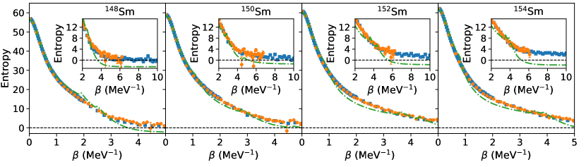
Figure 1: The canonical entropy as a function of inverse temperature $\beta$ for the even-mass samarium isotopes ^{148,150,152,154}Sm. For each isotope, the SPA+RPA entropy (orange circles) is compared with the SMMC entropy (blue squares) and the HFB entropy (green dashed-dotted line). The error bars on the SMMC and SPA+RPA results are statistical errors due to the Monte Carlo sampling. The insets show an expanded scale at large values of $\beta$.

In the SPA+RPA, we calculate the canonical energy $E_{c}$ and heat capacity $C$ with the Monte Carlo method described in Sec. III.1, using Eqs. (37) and (41), respectively. We define a sweep as an update of each of the four integration variables $x$. For each $\beta$ value, we initially carry out 50 sweeps to make sure that the Monte Carlo walk is thermalized, i.e., the walk has reached a representative region of the configuration space according to the weight function $W(x)$. We then calculate the observables every 70 sweeps to ensure that their values are sufficiently decorrelated. In the Supplemental Material repository, we show that these numbers of sweeps yield acceptable thermalization and decorrelation supp . We use $\sim 1000-2000$ samples per $\beta$ value in the calculation of the observables.

From the energy $E_{c}(\beta)$, we calculate $\ln Z_{c}(\beta)$ using Eq. (39) and the canonical entropy $S_{c}(\beta)$ using Eq. (30). We then calculate the state density from Eq. (29). The Monte Carlo results and computer codes used to analyze them are provided in the Supplemental Material repository supp .

Below, we compare the SPA+RPA results with exact (up to statistical errors) SMMC results and with mean-field finite-temperature HFB results. In the SMMC, we calculate the thermal canonical energy as the expectation value of the Hamiltonian $\langle\hat{H}\rangle$ for fixed proton and neutron numbers; for details, see Ref. alhassid_rev . We also calculate the heat capacity using the method of Ref. liu2001 , which reduces significantly the statistical errors. Using the canonical energy and heat capacity, we obtain the entropy and state density using Eqs. (30) and (29), respectively.

For the finite-temperature HFB, we calculate the self-consistent HFB solution at each temperature using the code of Ref. ryssens_hfshell , together with the particle-number-projected partition function using the method of Ref. fanto2017 . We then apply Eqs. (31), (30), (29) to obtain, respectively, the energy, entropy, and state density.

IV.1 Even-mass samarium isotopes

In Fig. 1, we show the canonical entropy $S_{c}$ as a function of inverse temperature $\beta$ for the SPA+RPA (orange circles), SMMC (blue squares), and HFB (green dashed-dotted line) for the even-mass samarium isotopes ^{148,150,152,154}Sm. The SPA+RPA entropies are shown up to values of $\beta$ close to the value above which the approximation breaks down. For each of the isotopes, we find the SPA+RPA entropy to be in excellent agreement with the SMMC entropy. The two kinks in the HFB entropy for ¹⁴⁸Sm indicate the proton and neutron pairing phase transitions, and the additional kink at lower $\beta$ for the other isotopes is due to the shape phase transition from a spherical to a deformed mean-field solution.

At $\beta$ values above the shape transition, the HFB entropy significantly underestimates the SPA+RPA and SMMC entropies because the HFB does not describe the contribution of rotational bands that are built on intrinsic mean-field band heads alhassid2016 . The SPA+RPA restores the rotational symmetry that is broken in the HFB and thus reproduces this rotational enhancement of the entropy. Furthermore, in the pairing phase, the HFB entropy becomes unphysically negative because of the inherent breaking of particle-number conservation in the HFB approximation fanto2017 . In contrast, the SPA+RPA entropy remains nonnegative (within statistical errors) because the SPA+RPA repairs the intrinsic violation of particle-number conservation. Finally, as the neutron number increases, the SPA+RPA and SMMC entropies remain nonzero to increasingly large values of $\beta$, indicating the presence of a rotational enhancement down to lower temperatures in nuclei with larger deformation.

We used the partition function extrapolation method summarized in Sec. III.2 to estimate the ground-state energy from the SPA+RPA partition function above the breakdown temperature of the approximation. For ^148,150Sm, we used the composite formula (45) in the second step of the fit, whereas for ^152,154Sm the back-shift parameter $\Delta$ is negative, and it was simpler to use the BBF formula (46). In Table 1, we compare the SPA+RPA ground-state energy estimates to the SMMC and HFB ground-state energies. We calculated the SMMC ground-state energies by taking a weighted average of the thermal energy at large $\beta$ values ($\beta\approx 8-20$ MeV^-1). Table 1 shows that the SPA+RPA misses at most $\sim$600 keV of ground-state correlation energy, whereas the HFB misses a few MeV of correlation energy in each isotope. The agreement between the SPA+RPA estimate and the SMMC ground-state energy improves with decreasing deformation, and the two agree with each other for the spherical isotope ¹⁴⁸Sm. In Table 2, we show the parameters $a,\Delta,E_{M}$ of the state density formulas obtained from the ground-state energy fits.

Table 1: The ground-state energies (in MeV) for the SMMC, SPA+RPA, and HFB for ^{148,150,152,154}Sm. The SPA+RPA estimates are obtained with the partition function extrapolation method described in Sec. III.2, with errors arising from the $\chi^{2}$ fit to the SPA+RPA partition function data. The SMMC values are obtained by taking a weighted average of the thermal energies at large $\beta$ values.

	SMMC	SPA+RPA	HFB
148Sm	-234.180 $\pm$ 0.016	-234.131 $\pm$ 0.021	-230.979
150Sm	-254.019 $\pm$ 0.014	-253.859 $\pm$ 0.015	-251.127
152Sm	-273.756 $\pm$ 0.010	-273.242 $\pm$ 0.017	-271.153
154Sm	-293.292 $\pm$ 0.010	-292.680 $\pm$ 0.017	-290.449

Table 2: The parameters obtained from the partition function extrapolation method discussed in Sec. III.2 applied to the SPA+RPA. For ^148,150Sm, we used the composite formula (45) in the second step of the fit, while for ^152,154Sm, we used the BBF (46).

	$a$ (MeV-1)	$\Delta$ (MeV)	$E_{M}$ (MeV)
148Sm	17.09 $\pm$ 0.11	1.07 $\pm$ 0.03	1.452
150Sm	18.28 $\pm$ 0.06	0.62 $\pm$ 0.02	0.95
152Sm	19.14 $\pm$ 0.10	-0.17 $\pm$ 0.03	–
154Sm	18.89 $\pm$ 0.13	-0.38 $\pm$ 0.03	–

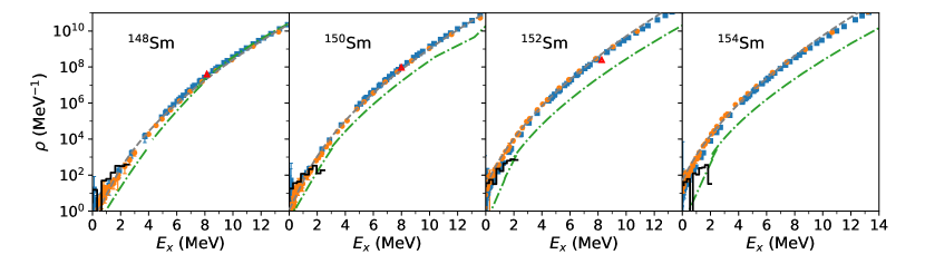
Figure 2: The state density $\rho$ as a function of excitation energy $E_{x}$ for the even-mass samarium isotopes. The SPA+RPA state density (orange circles) is compared with the SMMC density (blue squares) and the HFB density (green dashed-dotted lines) for each isotope. The grey dashed lines show the composite formula (45) for ^148,150Sm and the BBF (46) for ^152,154Sm, with the parameters from Table 2 (see text). Experimental neutron resonance data (red triangles) and low-energy level counting data (black histograms) are also shown. The error bars show statistical errors in the SPA+RPA and SMMC results.

Using the ground-state energies in Table 1, we calculated the SMMC, SPA+RPA, and HFB state densities for ^{148,150,152,154}Sm. Fig. 2 shows these densities, using a similar convention as in Fig. 1. In each isotope, the SPA+RPA state density is in good agreement with the SMMC state density. In contrast, the HFB state density significantly underestimates the SMMC and SPA+RPA densities. As the neutron number increases, the enhancement of the SMMC and SPA+RPA state densities over the HFB state density persists to higher excitation energy. This enhancement originates in the contribution of rotational bands that are included in the SMMC and SPA+RPA densities but are not described by the HFB approximation. We observe an additional enhancement of the SPA+RPA and SMMC state densities over the HFB density at very low excitation energies, which is due to the unphysical negative entropy in the pairing phase of the HFB. This latter enhancement is particularly apparent in the spherical nucleus ¹⁴⁸Sm.

In Fig. 2 we also compare the calculated state densities with experimental state densities obtained from level counting at low excitation energies nndc (black histograms) and the average $s$-wave neutron resonance spacings $D_{0}$ at the neutron threshold ripl (red triangles). We used a spin cutoff model bethe1937 ; ericson1960 with the rigid-body moment of inertia to convert $D_{0}$ values to state densities. The agreement between the data and the SPA+RPA and SMMC state densities is good overall, in particular for ^148,150Sm. In ^152,154Sm, the calculated densities overestimate the experimental data. In contrast, the mean-field HFB densities do not agree well with the experimental data.

In Fig. 2 we also show the phenomenological composite or BBF state densities calculated with the parameters reported in Table 2. We find good agreement between these fitted parameterizations and the SPA+RPA state densities. This agreement demonstrates that the partition function extrapolation method to extract the ground-state energy described in Sec. III.2 is reliable.

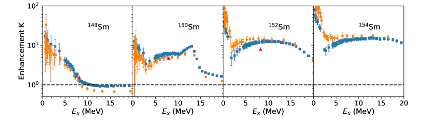
Figure 3: The enhancement factor $K=\rho/\rho_{\rm HFB}$ for the SPA+RPA (orange circles), the SMMC (blue squares), and the neutron resonance data (red triangles) for the even-mass samarium isotopes. The error bars indicate statistical errors from the Monte Carlo sampling.

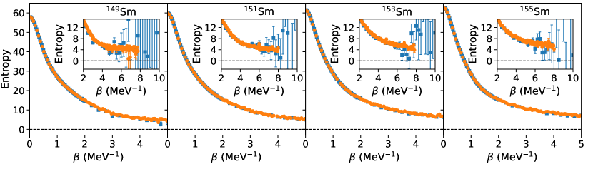
Figure 4: The canonical entropy as a function of inverse temperature $\beta$ for the odd-mass samarium isotopes ^{149,151,153,155}Sm. The SPA+RPA entropy (orange circles) is compared with the SMMC entropy (blue squares) for each isotope. The error bars show statistical errors arising from the Monte Carlo sampling. The insets show an expanded scale at large values of $\beta$.

To demonstrate even more clearly how well the SPA+RPA describes correlations that are missing in the mean-field approximation, we show in Fig. 3 the state density enhancement factor $K=\rho/\rho_{\rm HFB}$ for the SMMC (blue squares) and SPA+RPA (orange circles). The SPA+RPA enhancement factors are in good agreement with the SMMC enhancement factors. In the spherical nucleus ¹⁴⁸Sm, the enhancement factor differs significantly from one only at the lowest excitation energies and is due entirely to the unphysical negative entropy in the pairing phase of the HFB. In the deformed isotopes ^150,152,154Sm, a significant rotational enhancement of $\sim 10$ appears and persists to increasing excitation energy as the neutron number increases. This change in the enhancement factor indicates the crossover from pairing-dominated to rotational collectivity in the chain of samarium isotopes ozen2013 ; gilbreth2018 ; mustonen2018 . Fig. 3 also shows that the SPA+RPA and SMMC results are in good agreement with the neutron resonance data (red triangles) in ^148,150Sm. The calculated enhancement factors somewhat overestimate the neutron resonance data in ¹⁵²Sm.

IV.2 Odd-mass samarium isotopes

Having established the accuracy of the SPA+RPA state densities for the even-mass samarium isotopes, we next benchmark the SPA+RPA state densities for the odd-mass samarium isotopes ^{149,151,153,155}Sm. In Fig. 4, we compare the SPA+RPA canonical entropy (orange circles) with the SMMC canonical entropy (blue squares) for the odd-mass isotopes. In each isotope, the SPA+RPA entropy is in excellent agreement with the SMMC entropy. The odd-mass sign problem leads to large fluctuations of the SMMC entropy at high values of $\beta$, as is shown in the insets of Fig. 4. The SPA+RPA entropy remains reliable to slightly lower temperatures than the SMMC entropy. Both the SPA+RPA and SMMC entropies appear to converge to a nonzero limit, indicating the magnetic degeneracy of the nonzero-spin ground state of the odd-mass system.

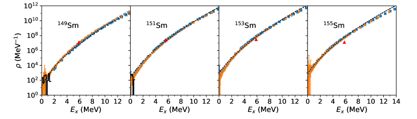
Figure 5: The state density as a function of excitation energy $E_{x}$ calculated with the SPA+RPA (orange circles) and SMMC (blue squares) for the odd-mass samarium isotopes ^{149,151,153,155}Sm. The BBF calculated with parameters obtained from fitting the SPA+RPA ground-state energies (grey dashed lines) and fitting the SMMC ground-state energies (black dotted lines) are also shown. Experimental neutron resonance data (red triangles) and low-energy level counting data (black histograms) are shown as well.

The projection on the odd number of neutrons introduces a Monte Carlo sign problem in the SMMC at low temperatures mukherjee2012 ; alhassid_rev that prevents the ground-state energy from being calculated directly. To obtain the SMMC and SPA+RPA state densities as functions of excitation energy, we used the partition function extrapolation method, which is summarized in Sec. III.2, to determine the ground-state energies $E_{0}$ in both approaches. We used the BBF (46) in the second step of the fits. Table 3 shows the extracted values of $E_{0}$ and the BBF state density parameters $a,\Delta$ for the SMMC and SPA+RPA. The agreement between the SMMC and SPA+RPA ground-state energy estimates is even better than for the even-mass isotopes, with the largest discrepancy of $\sim 300$ keV in ¹⁴⁹Sm.

Table 3: Ground-state energies $E_{0}$ and $a,\Delta$ values from fitting the BBF (46) to the SPA+RPA and SMMC excitation partition functions for the odd-mass samarium isotopes.

		$E_{0}$ (MeV)	$a$ (MeV-1)	$\Delta$ (MeV)
149Sm	SPA+RPA	-242.957 $\pm$ 0.008	18.36 $\pm$ 0.04	-0.13 $\pm$ 0.01
	SMMC	-243.327 $\pm$ 0.019	17.97 $\pm$ 0.04	-0.04 $\pm$ 0.02
151Sm	SPA+RPA	-262.913 $\pm$ 0.006	19.24 $\pm$ 0.07	-0.39 $\pm$ 0.02
	SMMC	-262.909 $\pm$ 0.047	18.63 $\pm$ 0.06	-0.77 $\pm$ 0.05
153Sm	SPA+RPA	-282.384 $\pm$ 0.005	19.57 $\pm$ 0.12	-0.84 $\pm$ 0.02
	SMMC	-282.449 $\pm$ 0.031	18.78 $\pm$ .09	-1.25 $\pm$ 0.05
155Sm	SPA+RPA	-301.949 $\pm$ 0.003	19.07 $\pm$ 0.12	-1.00 $\pm$ 0.03
	SMMC	-302.077 $\pm$ 0.021	18.27 $\pm$ 0.10	-1.39 $\pm$ 0.04

In Fig. 5, we compare the state densities calculated with the SMMC (blue squares) and SPA+RPA (orange circles). The results are in good agreement with each other and with available experimental data from level counting nndc (black histograms) and the average $s$-wave neutron resonance spacings ripl (red triangles). The agreement between the calculated and experimental state densities degrades somewhat as the neutron number increases and is of similar quality to the agreement found in Ref. ozen2015 using an interaction that included contributions from higher-order multipoles. We also show in Fig. 5 the BBF state densities calculated with the parameters tabulated in Table 3. These fitted BBF densities agree well with the calculated state densities.

V Conclusion and outlook

Here we benchmarked state densities calculated with the SPA+RPA in the CI shell model framework against exact (up to controllable statistical errors) SMMC state densities for a chain of samarium isotopes ^148-155Sm. We implemented a Monte Carlo method to calculate the canonical energy and heat capacity in the SPA+RPA, from which we determined the canonical entropy and state density. The SPA+RPA ground-state energy was estimated from the excitation partition function above the SPA+RPA breakdown temperature using the partition function extrapolation method ozen2020 .

We found good agreement between the SPA+RPA state densities and SMMC state densities for all the isotopes considered. For the even-mass samarium isotopes, we also calculated mean-field state densities using the finite-temperature HFB approximation. The main deficiencies of the mean-field approximation arise from the broken rotational symmetry in deformed nuclei and the inherent violation of particle-number conservation in the pairing condensate. Consequently, the mean-field approximation cannot reproduce the contribution of rotational bands that are characteristic of deformed nuclei and yields an unphysical negative entropy in the pairing phase of the HFB. The SPA+RPA resolves these deficiencies of the mean-field approximation. In particular, the SPA+RPA reproduces well the rotational collective enhancement of the state density relative to the mean-field density in deformed nuclei. This enhancement persists to higher excitation energies as the neutron number increases, showing that the importance of rotational collectivity increases with deformation. Overall, our results show that the SPA+RPA provides state densities in the CI shell model framework that are in agreement with exact SMMC densities.

A significant limitation of the SPA+RPA method is the computational cost of diagonalizing the RPA matrix at each sampled configuration of the static fields. The dimension of the RPA matrix scales as $\sim N_{s,p}^{2}+N_{s,n}^{2}$ (where $N_{s,p(n)}$ is the number of proton(neutron) single-particle states), and the cost of diagonalizing this matrix scales as the cubic power of this dimension. Calculating the canonical energy and heat capacity in the SMMC scales as a lower power of the number of single-particle states, specifically as $\sim N_{s}^{4}$ for each particle species. It would therefore be useful to investigate methods for speeding up the calculation of the RPA correction factor. One such method was proposed in Ref. kaneko2005 .

In comparing the SPA+RPA to the SMMC, it is also useful to consider the limits of the applicability of each method. The SPA+RPA method requires that the single-particle Hamiltonian $\hat{h}_{\sigma}$ in Eq. (3) be a Hermitian operator for any configuration $\sigma$ of the static auxiliary fields. This condition is guaranteed if all terms in the Hamiltonian are attractive when written in the separable form $\hat{O}_{\alpha}^{2}$ of Eq. (1), where each operator $\hat{O}_{\alpha}$ is Hermitian. Moreover, this condition guarantees that, at temperatures above the breakdown temperature of the SPA+RPA, the weight function $W(\sigma)$ of the Monte Carlo method discussed in Sec. III.1 and the RPA correction factor $C_{\eta}(\sigma)$ are both positive definite for any static field configuration $\sigma$. Consequently, $W(\sigma)$ can be used as a weight function to sample the static fields, and the Monte Carlo method described in Sec. III.1 will not have a sign problem. In contrast, for the SMMC method to have a good Monte Carlo sign, the Hamiltonian must be invariant under time reversal, and all of its interaction terms must be attractive when written as a sum over terms of the form $\{\hat{O}_{\alpha},\bar{O}_{\alpha}\}$ where $\bar{O}_{\alpha}$ is the time reverse of $\hat{O}_{\alpha}$  alhassid_rev ; lang1993 ; alhassid1994 . It can be shown that the time-reversal and Hermitian conjugate of a tensor one-body density operator are related by a sign. Thus, in some cases, either the SPA+RPA or SMMC would have good sign while the other method would have a sign problem, and the two methods would complement each other. Furthermore, the SPA+RPA can be applied if time-reversal symmetry is broken, e.g., in the presence of a cranking term $-\omega\hat{J}_{i}$ ($i=x,y,z$), which would cause a sign problem in the SMMC.

A method for approximately including repulsive interactions in the SPA+RPA framework was proposed in Ref. canosa1997 . It would be interesting to benchmark this method for realistic nuclear interactions that include repulsive components.

Finally, statistical reaction codes require as input spin- and parity-dependent level densities, rather than just state densities. To calculate these level densities, it is necessary to extend the SPA+RPA formalism to include spin and parity projections.

References

- (1) W. Hauser and H. Feshbach, Phys. Rev. 87, 366 (1952).
- (2) A. J. Koning and D. Rochman, Nucl. Data Sheets 113, 2841 (2012).
- (3) M. Mumpower, R. Surman, G. C. McLaughlin, and A. Aprahamian, Prog. Part. Nucl. Phys. 86, 86 (2016).
- (4) R. Surman, M. Mumpower, R. Sinclair, K. L. Jones, W. R. Hix, and G. C. McLaughlin, AIP Advances 4, 041008 (2014).
- (5) P. Denissenkov, G. Perdikakis, F. Herwig, H. Schatz, C. Ritter, M. Pignatari, S. Jones, S. Nikas, and A. Spyrou, J. Phys. G 45, 055203 (2018).
- (6) J. Carlson et al., Prog. Part. Nucl. Phys. 94, 68 (2017).
- (7) A. Schiller, L. Bergholt, M. Guttormsen, E. Melby, J. Rekstad, and S. Siem, Nucl. Instrum. Methods A 447, 498 (2000).
- (8) A. Voinov, M. Guttormsen, E. Melby, J. Rekstad, A. Schiller, and S. Siem, Phys. Rev. C 63, 044313 (2001).
- (9) A. V. Voinov et al., Phys. Rev. C 99, 054609 (2019).
- (10) A. Spyrou, S. N. Liddick, A. C. Larsen, M. Guttormsen, K. Cooper, A. C. Dombos, D. J. Morrissey, F. Naqvi, G. Perdikakis, and S. J. Quinn, Phys. Rev. Lett. 113, 232502 (2014).
- (11) M. Herman, R. Capote, B. V. Carlson, P. Obložinský, M. Sin, A. Trkov, H. Wienke, and V. Zerkin, Nucl. Data Sheets 108, 2655 (2007).
- (12) S. Hilaire and S. Goriely, Nucl. Phys. A 779, 63 (2006).
- (13) S. Goriely, S. Hilaire, and A. J. Koning, Phys. Rev. C 78, 064307 (2008).
- (14) S. Hilaire, M. Girod, S. Goriely, and A. J. Koning, Phys. Rev. C 86, 064317 (2012).
- (15) Y. Alhassid, L. Fang, and H. Nakada, Phys. Rev. Lett. 101, 082501 (2008).
- (16) C. Özen, Y. Alhassid, and H. Nakada, Phys. Rev. Lett. 110, 042502 (2013).
- (17) M. Bonett-Matiz, A. Mukherjee, and Y. Alhassid, Phys. Rev. C 88, 011302 (2013).
- (18) C Özen, Y. Alhassid, and H. Nakada, Phys. Rev. C 91, 034329 (2015).
- (19) Y. Alhassid, in Emergent Phenomena in Atomic Nuclei from Large-Scale Modeling: a Symmetry-Guided Perspective, ed. K. D. Launey, (World Scientific, Singapore, 2017), pp. 267-298.
- (20) G. H. Lang, C. W. Johnson, S. E. Koonin, and W. E. Ormand, 48, 1518 (1993).
- (21) Y. Alhassid, D. J. Dean, S. E. Koonin, G. Lang, and W. E. Ormand, Phys. Rev. Lett. 72, 613 (1994).
- (22) K. Mon and J. French, Annals of Physics 95, 90 (1975).
- (23) M. Horoi, M. Ghita, and V. Zelevinsky, Phys. Rev. C 69, 041307 (2004).
- (24) R. Sen’kov and V. Zelevinsky, Phys. Rev. C 93, 064304 (2016).
- (25) N. Shimizu, Y. Utsuno, Y. Futamura, T. Sakurai, T. Mizusaki, and T. Otsuka, Phys. Lett. B 753, 13 (2016).
- (26) W. E. Ormand and B. A. Brown, Phys. Rev. C 23, 014315 (2020).
- (27) A. K. Kerman and S. Levit, Phys. Rev. C 24, 1029 (1981).
- (28) B. Lauritzen, P. Arve, and G. F. Bertsch, Phys. Rev. Lett. 61, 2835 (1988).
- (29) G. Puddu, P. F. Bortignon, and R. A. Broglia, Phys. Rev. C 42, R1830 (1990).
- (30) B. Lauritzen, G. Puddu, P. F. Bortignon, and R. A. Broglia, Phys. Lett. B 246, 329 (1990).
- (31) G. Puddu, P. F. Bortignon, and R. A. Broglia, Ann. Phys. 206, 409 (1991).
- (32) G. Puddu, Phys. Rev. C 47, 1067 (1993).
- (33) H. Attias and Y. Alhassid, Nucl. Phys. A 625, 565 (1997).
- (34) R. Rossignoli, N. Canosa, and P. Ring, Phys. Rev. Lett. 80, 1853 (1998).
- (35) K. Kaneko et al., Phys. Rev. C 74, 024325 (2006).
- (36) K. Kaneko and A. Schiller, Phys. Rev. C 75, 044304 (2007).
- (37) K. N. Nesterov and Y. Alhassid, Phys. Rev. B 87, 014515 (2013).
- (38) C. N. Gilbreth, Y. Alhassid, and G. F. Bertsch, Phys. Rev. C 97, 014315 (2018).
- (39) M. T. Mustonen, C. N. Gilbreth, Y. Alhassid, and G. F. Bertsch, Phys. Rev. C 98, 034317 (2018).
- (40) Y. Alhassid and C. Özen, in preparation.
- (41) N. Canosa and R. Rossignoli, Phys. Rev. C 56, 791 (1997).
- (42) J. Hubbard, Phys. Rev. Lett. 3, 77 (1959).
- (43) R. Stratonovich, Dokl. Akad. Nauk. S. S. S. R. 115, 1097 (1957).
- (44) P. Ring, L. M. Robledo, J. L. Egido, and M. Faber, Nucl. Phys. A 419, 261 (1984).
- (45) A. Bohr and B. R. Mottelson, Nuclear Structure, Vol. 1 (Benjamin, New York, 1969).
- (46) Y. Alhassid, G. F. Bertsch, C. N. Gilbreth, and H. Nakada, Phys. Rev. C 93, 044320 (2016).
- (47) Y. Alhassid, G. F. Bertsch, L. Fang, and S. Liu, Phys. Rev. C 72, 064326 (2005).
- (48) R. Rossignoli, Phys. Rev. C 54, 1230 (1996).
- (49) J. Gubernatis, N. Kawashima, and P. Werner, Quantum Monte Carlo Methods: Algorithms for Lattice Models (Cambridge University Press, Cambridge, 2016).
- (50) P. Young, Everything You Wanted to Know About Data Analysis and Fitting but Were Afraid to Ask, SpringerBriefs in Physics (Springer, Cham, 2015).
- (51) The Supplemental Material repository contains further discussion of the Monte Carlo algorithm and analysis method, as well as the data files and computer codes required to reproduce the figures shown. This repository is available upon email request sent to paul.fanto@yale.edu.
- (52) A. Mukherjee and Y. Alhassid, Phys. Rev. Lett. 109, 032503 (2012).
- (53) A. Gilbert and A. G. W. Cameron, Can. J. Phys. 43, 1446 (1965).
- (54) W. Dilg, W. Schantl, H. Vonach, and M. Uhl, Nucl. Phys. A 217, 269 (1973).
- (55) Y. Alhassid, G. F. Bertsch, D. J. Dean, and S. E. Koonin, Phys. Rev. Lett. 77, 1444 (1996).
- (56) S. Liu and Y. Alhassid, Phys. Rev. Lett. 87, 022501 (2001).
- (57) W. Ryssens and Y. Alhassid, in preparation.
- (58) P. Fanto, Y. Alhassid, and G. F. Bertsch, Phys. Rev. C 96, 014305 (2017).
- (59) National Nuclear Data Center, information extracted from the NuDat 2 database, http://www.nndc.bnl.gov/nudat2/
- (60) R. Capote et al., Nucl. Data Sheets 110, 3107 (2009).
- (61) H.A. Bethe, Rev. Mod. Phys. 9, 69 (1937).
- (62) T. Ericson, Advances in Physics 9, 425 (1960).
- (63) K. Kaneko and M. Hasegawa, Phys. Rev. C 72, 061306 (2005).