Switchable Deep Beamformer

Abstract

Recent proposals of deep beamformers for ultrasound imaging (US) using deep neural networks have attracted significant attention as computational efficient alternatives to adaptive and compressive beamformers. Moreover, deep beamformers are versatile in that image post-processing algorithms can be combined with the beamforming. Unfortunately, in the current technology, a separate beamformer should be trained and stored for each application, demanding significant scanner resources. To address this problem, here we propose a switchable deep beamformer that can produce various types of output such as DAS, speckle removal, deconvolution, etc., using a single network with a simple switch. In particular, the switch is implemented through Adaptive Instance Normalization (AdaIN) layers, so that distinct outputs can be generated by merely changing the AdaIN code. Experimental results using B-mode focused ultrasound confirm the flexibility and efficacy of the proposed method for various applications.

I Introduction

Ultrasound (US) is one of the most versatile medical imaging modalities. Thanks to its fast frame rate and radiation free nature, it is the first choice for applications such as fetal imaging, cardiac imaging, etc.

The image generation process in US involves scanning and reconstruction steps. In focused mode, the region of interest (ROI) is scanned in a line-by-line fashion, while in planewave (PW) mode, the full ROI is scanned at once. For the reconstruction, out-of-phased RF signals are accumulated after back-propagation. For example, the basic steps of conventional delay-and-sum (DAS) beamforming pipeline are: (1) time-of-flight correction in which RF measurements are shifted in time, and (2) the summation of the time-corrected signal.

While the DAS beamformer is widely used due to its simplicity and robust reconstruction performance, it often suffers from poor resolution due to signal side-lobes. Moreover, DAS images are usually associated with image artifacts such as speckles, blurring, etc., whose removal have been one of the main research topics in US research. However, existing approaches using adaptive beamforming techniques [1, 2, 3, 4, 5, 6, 7, 8, 9] and compressed sensing [10, 11, 12, 13] are computationally expensive and sensitive to hyperparameters, so a recent trend is using deep learning approaches in the design of beamformers and image processing algorithms [14, 15, 16, 17, 18, 19].

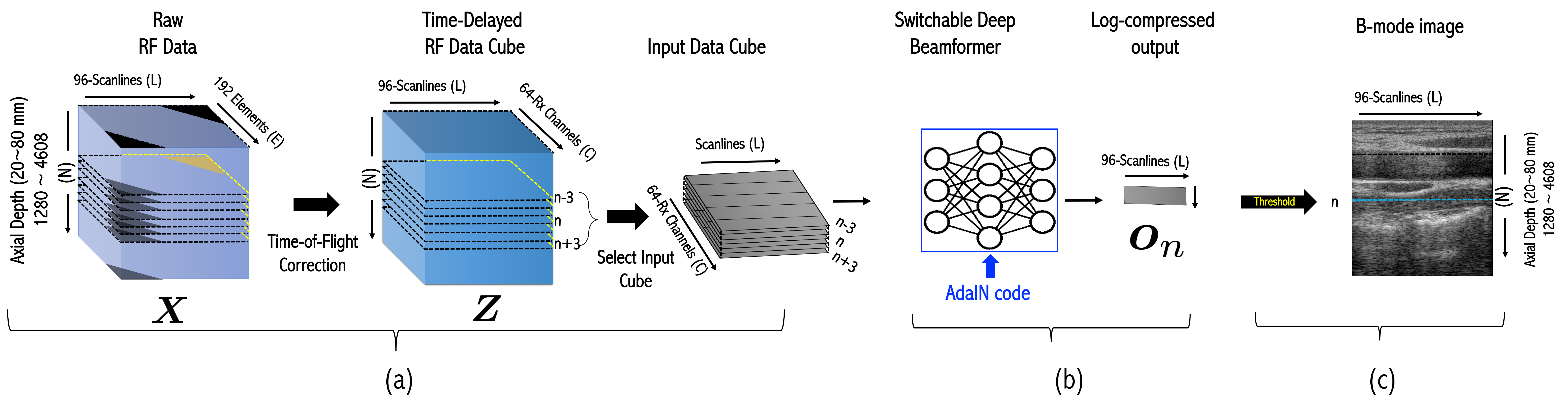
Figure 1: Data processing pipeline for the proposed switchable deep beamformer. (a) Neural network input preparation step, (b) switchable deep beamformer, and (c) thresholding and display step for visualization.

For example, Luchies and Byram [14] proposed a deep learning based frequency domain beamforming method for off-axis scattering suppression. In [16], a beamformer is designed to produce speckle-free images from channel data. A major limitation of these methods [14, 16] is that the training data are usually obtained from simulation phantom and therefore recovery of accurate images is challenging especially for in-vivo data. On the other hand, recent deep beamformers [17, 18, 19] utilizes in vivo data as reference target for supervised training. For example, in the universal deep beamformer [17, 18], neural network is trained to generate high resolution DAS, minimum variance beamformer (MVBF), and deconvolution ultrasound outputs from channel data. In another work [19], a neural network was trained to mimic the output of MV beamformer for fast beamforming.

Although deep beamfomers provide impressive performance and ultra-fast reconstruction, one of the downsides of the deep beamformers is that a distinct model is needed for each type of desired output. For instance, to obtained DAS output, a model is needed which mimics DAS; similarly, for MVBF a separate model is needed. Although the architecture of the model will be the same, separate weight is needed to be stored for each output type. Additionally, to enable a deep beamformer to generate output that matches to several post processing results, such as deblurring or speckle reduction, etc., it further increases the number of models to be stored.

To address this issue, here we propose a novel switchable deep beamformer architecture using adaptive instance normalization (AdaIN) layers. AdaIN was originally proposed as an image style transfer method, in which the mean and variance of the feature vectors are replaced by those of the style reference image [20]. Recently, AdaIN has attracted significant attention as a powerful component to control generative models. For example, in the StyleGAN [21], the network generated various realistic faces with the same inputs by simply adjusting the mean and variance of the feature maps using AdaIN. In StarGANv2 [22], AdaIN plays the key role in converting styles from input images. Furthermore, a recent study [23] has shown that the change of style by AdaIN is not a cosmetic change but a real one thanks to the important link to the optimal transport [24, 25] between the feature vector spaces.

Inspired by the success of AdaIN and its theoretical understanding, one of the most important contributions of this work is to demonstrate that a single deep beamformer with AdaIN layers can learn target images from various styles. Here, a “style” refers to a specific output processing, such as DAS, MVBF, deconvolution image, despeckled images, etc. Once the network is trained, the deep beamformer can then generate various style output by simply changing the AdaIN code. Furthermore, the AdaIN code generation can be easily done with a very light AdaIN code generator, so the additional memory overhead at the training step is minimal. Once the neural network is trained, we only need the AdaIN codes without the generator, which makes the system even simpler. As such, our switchable deep beamformer can be considered as the first, fully adaptive multi-purpose deep beamformer for the reconstruction of high-quality medical ultrasound images.

This paper is organized as follows. The deep beamformer and AdaIN are first reviewed in Section II, after which we explain how these techniques can be synergistically combined to produce a switchable deep beamformer in Section III. Section IV describes the data set and experimental setup. Experimental results are provided in Section V, which is followed by Conclusions in Section VI.

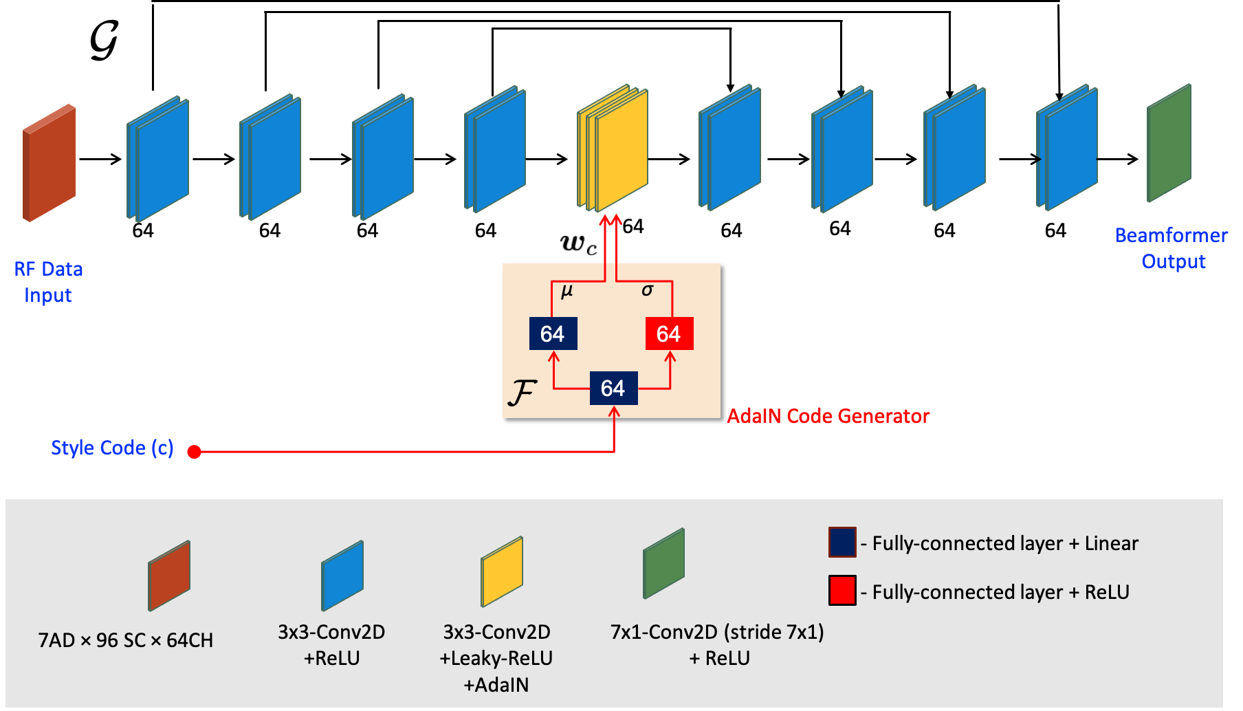
Figure 2: Architecture of our switchable deep beamformer. Adaptive instance normalization (AdaIN) layer is added at the bottleneck layer, for which AdaIN code is generated by a separate AdaIN code generator network.

II Related works

II-A Deep Beamformer

Among the various forms of deep beamformers, here we review the universal deep beamformer (DeepBF) [17, 18] as a representative form of deep beamformer, since our switchable deep beamformer is built upon this architecture.

In US, measured RF data is usually given as a three-dimensional cube ${\bm{X}}\in{\mathbb{R}}^{L\times N\times E}$ as shown in Fig. 1(a), where $L,N,$ and $E$ denote the number of scan lines (or transmit events (TE)), depth planes, and the number of probe elements, respectively. The time-delay corrected data cube ${\bm{Y}}\in{\mathbb{R}}^{L\times N\times E}$ is similarly denoted by ${\bm{Y}}=[{\bm{y}}_{l,n}]_{l,n}$, where

$${\bm{y}}_{l,n}=\begin{bmatrix}y_{l,n}[0]&y_{l,n}[1]&\cdots&y_{l,n}[E-1]\end{bmatrix}^{\top}\in{\mathbb{R}}^{E}$$ (1)

Then, the received channel data can be explicitly modeled as ${\bm{Z}}=[{\bm{z}}_{l,n}]_{l,n}$, where

$${\bm{z}}_{l,n}=\begin{bmatrix}z_{l,n}[0]&z_{l,n}[1]&\cdots&z_{l,n}[{J}-1]\end{bmatrix}^{\top}\in{\mathbb{R}}^{J}$$ (2)

and

$$z_{l,n}[i]=y_{l,n}[i+d_{l}]$$ (3)

where $J$ is the aperture size, and $d_{l}$ denotes the specific detector offset to indicate the active channel elements, which is determined for each scan line index $l$. This implies that the dark triangular regions in ${\bm{X}}$ as shown Fig. 1(a), which correspond to inactive receiver elements, are removed in constructing ${\bm{Z}}$.

The standard delay and sum (DAS) beamformer for the $l$-th scanline at the depth sample $n$ can be expressed as

$${u}_{l,n}=\frac{1}{J}\mathbf{1}^{\top}{\bm{z}}_{l,n}$$ (4)

where $\mathbf{1}$ denotes a $J$-dimensional column-vector of ones. On the other hand, DeepBF [17, 18] generates multiple scan-lines in a depth simultaneously using multiple-depth channel data:

$${\bm{o}}_{n}~{}=\mathcal{G}_{\bm{\Theta}}\left({\bm{Z}}_{n}\right), {\bm{o}}_{n}\in\mathcal{O}$$ (5)

where ${\bm{o}}_{n}$ denotes the output at the depth $n$:

$${\bm{o}}_{n}=\begin{bmatrix}o_{0,n}\\ \vdots\\ o_{L-1,n}\end{bmatrix}$$ (6)

with $o_{l,n}$ referring to the target image at the $l$-th scan line and the depth $n$, and $\mathcal{G}_{\bm{\Theta}}$ is a neural network parameterized by ${\bm{\Theta}}$, ${\bm{Z}}_{n}$ is a channel data collected from, for example, seven depth planes around the depth $n$:

$${\bm{Z}}_{n}=\begin{bmatrix}{\bm{z}}_{n-3}&\cdots&{\bm{z}}_{n}&\cdots&{\bm{z}}_{n+3}\end{bmatrix}\in\mathcal{Z}$$ (7)

where ${\bm{z}}_{n}$ is defined as:

$${\bm{z}}_{n}=\begin{bmatrix}z_{0,n}\\ \vdots\\ z_{L-1,n}\end{bmatrix}$$ (8)

Then, the resulting neural network training is given by

$$\min_{{\bm{\Theta}}}\sum_{t,n}\|{\bm{o}}_{n}^{(t)}-\mathcal{G}_{\bm{\Theta}}({\bm{Z}}_{n}^{(t)})\|_{2}^{2},$$ (9)

where $({\bm{Z}}_{n}^{(t)},{\bm{o}}_{n}^{(t)})$ denotes the input channel data and the target image data at the depth index $n$, and the superscript index $t$ is the training data set index. In fact, the training data can be obtained not only from different experiment data but also from different depth in the same frame [17, 18].

One of the important advantages of the deep beamformer is that depending on the target data ${\bm{o}}_{n}$, the neural network parameter ${\bm{\Theta}}$ is trained accordingly to mimic target data. In [17, 18], the authors used the DAS, minimum variance beamformer (MVBF), and deconvolution images as targets, so that deep beamformer can directly produce target domain images. However, as discussed before, separate network parameter ${\bm{\Theta}}$ should be stored for each target domain, demanding significant amount of scanner resources.

II-B Adaptive Instance Normalization (AdaIN)

AdaIN [20] is an extension of instance normalization [26], which goes beyond the classical role of the normalization methods for image style transfer. The key idea of AdaIN is that latent space exploration is possible by adjusting the mean and variance of the feature map. Specifically, style transfer is performed by matching the mean and variance of the feature map of the input image to those of the style image [20].

More specifically, let a multi-channel feature map be represented by

$${\bm{U}}= \begin{bmatrix}{\bm{u}}_{1}&\cdots&{\bm{u}}_{P}\end{bmatrix}\in{\mathbb{R}}^{HW\times P},$$ (10)

where ${\bm{u}}_{i}\in{\mathbb{R}}^{HW\times 1}$ refers to the $i$-th column vector of ${\bm{U}}$, which represents the vectorized feature map of size of $H\times W$ at the $i$-th channel. Suppose, furthermore, the corresponding feature map for the style reference image is given by

$${\bm{V}}= \begin{bmatrix}{\bm{v}}_{1}&\cdots&{\bm{v}}_{P}\end{bmatrix}\in{\mathbb{R}}^{HW\times P}.$$ (11)

Then, AdaIN changes the feature data for each channel using the following transform:

$${\bm{z}}_{i} =\mathcal{T}({\bm{u}}_{i},{\bm{v}}_{i}),\quad i=1,\cdots,P$$ (12)

where

$$\mathcal{T}({\bm{u}},{\bm{v}}):=\frac{\sigma({\bm{v}})}{\sigma({\bm{u}})}\left({\bm{u}}-\mu({\bm{u}})\bm{1}\right)+\mu({\bm{v}})\bm{1},\quad$$ (13)

where $\bm{1}\in{\mathbb{R}}^{HW}$ is the $HW$-dimensional vector composed of 1, and $\mu({\bm{u}})$ and $\sigma({\bm{u}})$ are the mean and standard deviation (std) for ${\bm{u}}\in{\mathbb{R}}^{HW}$, which are computed by:

$$\mu({\bm{u}})=\frac{1}{HW}\bm{1}^{\top}{\bm{u}},~{} \sigma({\bm{u}})=\sqrt{\frac{1}{HW}\|{\bm{u}}-\mu\bm{1}\|^{2}}$$ (14)

The AdaIN transform in (13) has an important link to optimal transport [24, 25]. Specifically, consider the optimal transport scheme between two probability spaces $\mathcal{U}\subset{\mathbb{R}}^{HW}$ and $\mathcal{V}\subset{\mathbb{R}}^{HW}$, equipped with the Gaussian probability measure $\mu\sim\mathcal{N}({\bm{m}}_{U},{\bm{\Sigma}}_{U})$ and $\nu\sim\mathcal{N}({\bm{m}}_{V},{\bm{\Sigma}}_{V})$, respectively, where ${\bm{m}}_{U}$ and ${\bm{\Sigma}}_{U}$ denote the mean vector and the covariance matrix, respectively. Then, a recent study [23] showed that the optimal transport map from the measure $\mu$ to the measure $\nu$ with respect to Wasserstein-2 distance is given by

$$T_{\mu\rightarrow\nu}({\bm{u}})={\bm{m}}_{V}+{\bm{\Sigma}}_{U}^{-\frac{1}{2}}\left({\bm{\Sigma}}_{U}^{\frac{1}{2}}{\bm{\Sigma}}_{V}{\bm{\Sigma}}_{U}^{\frac{1}{2}}\right)^{\frac{1}{2}}{\bm{\Sigma}}_{U}^{-\frac{1}{2}}({\bm{u}}-{\bm{m}}_{U})$$ (15)

Therefore, if we assume the i.i.d. distribution, i.e.

$${\bm{m}}_{U}=\mu({\bm{u}})\bm{1},{\bm{\Sigma}}_{U}=\sigma({\bm{u}}){\bm{I}}, {\bm{m}}_{V}=\mu({\bm{v}}),{\bm{\Sigma}}_{V}=\sigma({\bm{v}}){\bm{I}}$$ (16)

where ${\bm{I}}$ is the identity matrix, then the optimal transport map in (15) can be simplified to

$$T_{\mu\rightarrow\nu}({\bm{u}})=\mu({\bm{v}})\bm{1}+\frac{\sigma({\bm{v}})}{\sigma({\bm{u}})}({\bm{u}}-\mu({\bm{u}})\bm{1})$$ (17)

which is equivalent to the AdaIN transform in (13). Therefore, the AdaIN transform can be considered the minimal cost transport path when converting one feature map to another under i.i.d. Gaussian feature map assumption.

III Theory

III-A Switchable Deep Beamformer using AdaIN Layers

Inspired by the observation that AdaIN is an optimal transport plan between the feature layers, our goal is to implement multi-purpose deep beamformer using a single baseline network followed by optimal transport layers to specific target distributions. Specifically, we use DeepBF [17, 18] as the baseline network and then use AdaIN transform to transport the features to different domain features.

More specifically, our switchable deep beamformer is formally defined as

$$\mathcal{G}(\cdot;\cdot):\mathcal{Z}\times\mathcal{W}\mapsto\mathcal{O}$$ (18)

where $\mathcal{Z}$ denotes the input RF channel data space composed of elements in (7), $\mathcal{O}$ is the output space for the beamformed data in (5), and $\mathcal{W}$ is the AdaIN code vector space, whose element ${\bm{w}}_{c}\in\mathcal{W}$ is generated by the AdaIN code generator ${\mathcal{F}}:{\mathbb{R}}\mapsto\mathcal{W}$ as

$${\bm{w}}_{c}={\mathcal{F}}(c)$$ (19)

where $c\in{\mathbb{R}}$ is the target style code. AdaIN code generator takes the style code representing a target domain, and generates the style mean and variance vectors required for that domain.

The architecture of the proposed switchable network $\mathcal{G}$ is shown in Fig. 2. In the baseline network, there are nine convolution blocks shown in blue and yellow colors. The blue blocks are composed of two convolution layer with ReLU activation function, while yellow block is composed of convolution, and Leaky ReLU blocks. All convolution layers uses stride value of $(1,1)$, with a 2-dimensional filter that has a dimension of $3\times 3$, expect the last layer shown in green color which uses $(7,1)$, with a 2-dimensional filter that has a dimension of $7\times 1$. As shown in Fig. 2, there exists an AdaIN layer at the bottleneck layer. The AdaIN layers take a mean vector and a variance vector as input. During the training phase, the AdaIN layers take the output vectors from the AdaIN code generator ${\mathcal{F}}$ in Fig. 2, which consists of fully connected layers and is trained together with the baseline neural network. For mean vector generation, a linear activation was used, whereas for the variance generation ReLU activation function was used to impose nonnegativity.

At the inference phase, we only use the baseline network $\mathcal{G}$ with the trained AdaIN codes $\{{\bm{w}}_{c}\}$, as the AdaIN code generator is no more necessary. Then, depending on the specific AdaIN code ${\bm{w}}_{c}$, our switchable deep beamformer output

$${\bm{o}}_{n}(c)=\mathcal{G}({\bm{Z}}_{n};{\bm{w}}_{c})$$

becomes an image with the $c$-style processing. Accordingly, the total memory requirement can be significantly reduced, and multiple processing can be done instanteneously by simply changing the code ${\bm{w}}_{c}$.

III-B Target Image Generations

As for multiple domain target reference data, in addition to DAS, we consider images from three post processing methods: (1) deconvolution (deblurring), (2) despeckle (denoising), and (3) the combination of the two. More details are as follows.

III-B1 DAS

In contrast to [17, 18] where IQ signal was used as target, for proposed switchable deep beamformer, we use the log-compressed absolute value of Hilbert transformed RF-sum as DAS target. Thanks to such changes, all the beamforming process is now learned by the neural network, and only thresholding for specific dynamic range can be performed for visualization as shown in Fig. 1(c). Similar log-compressed domain learning approaches are taken for other processing as follows.

III-B2 Deblurring

Deconvolution method can help reduce the blur to improve spatial resolution of an ultrasonic imaging system. As shown in Fig. 3, in US, a received signal is modeled as a convolution product of tissue reflectivity function (TRF) and point spread function (PSF), where TRF represents scatter’s acoustic properties, while the impulse response of the imaging system is modeled by PSF. The PSF is determined by the detector configurations, focused beam width, etc.

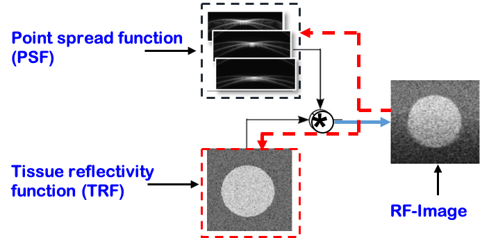
Figure 3: Block diagram of deconvolution ultrasound imaging.

Then, the unknown TRF $x$ is estimated by solving the following $l_{1}$ minimization problem:

$$\hat{x}=\operatorname*{arg\,min}_{x}||y-h\ast x||^{2}+\lambda_{1}||x||_{1}$$ (20)

where $y$ is the Hilbert transformed DAS RF-sum, $h$ is the PSF, $\lambda_{1}=0.02$ is a regularization parameter empirically chosen to control the tradeoff between sparsity and fitting fidelity.

In most practical cases, the complete knowledge of $h$ is not available, and therefore both unknown TRF $x$ and the PSF $h$ have to be estimated together, which is called the blind deconvolution problem. In this paper, we first estimate $h$ from $y$, and then $x$ is estimated based on $h$ [27]. To train the proposed switchable beamformer, a log-compressed absolute value, $20\log_{10}(|\hat{x}|)$, is used as a training reference.

III-B3 Denoising

Speckle noises are the granular patterns appears in US images, which is one of the a major reasons of quality degradation and removal of it can subsequently enhance the structural details in US images [28]. To design a speckle denoising beamformer, the log-absolute value of Hilbert transformed RF-sum was filtered using non-local low-rank (NLLR) method [28] to generate the reference data for supervised training. In NLLR as shown in Fig. 4, the image is pre-processed to generate a guidance map and later non-local filtering operations are performed on the candidate patches that are selected using that guidance map. For further refinement of filtered patches, a truncated nuclear norm (TWNN) and structured sparsity criterion are used [29, 30].

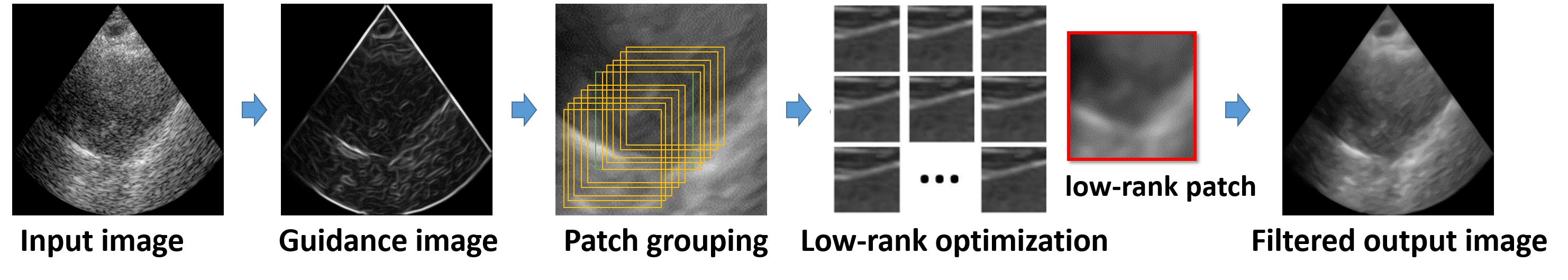
Figure 4: Block diagram of non-local low-rank (NLLR) filtering-based speckle removal method.

III-B4 Deconvolution + Denoising

To generate the deconvolution and despeckle reference images, we applied the NLLR filter on deconvoluted log-absolute RF-sum to generate deconvolution+despeckle output.

III-C Switchable Deep Beamformer Training

Let the data set $\{({\bm{Z}}_{n}^{(t)},{\bm{o}}_{n}^{(t)}(c))\}_{c,n,t}$ denotes the training data set collected across all depth planes $n$ and style $c$, where ${\bm{Z}}_{n}^{(t)}$ is defined in (7) and ${\bm{o}}_{n}(c)$ is the target image for a given style $c$ at the depth $n$. Then, the resulting neural network training for the proposed switchable deep beamformer is given by

$$\min_{\mathcal{G},{\mathcal{F}}}\sum_{c,t,n}\|{\bm{o}}_{n}^{(t)}(c)-\mathcal{G}({\bm{Z}}_{n}^{(t)};{\mathcal{F}}(c))\|_{2}^{2},$$ (21)

For each target style $c$, the AdaIN code generator network ${\mathcal{F}}$ expands the style input to produce desired size AdaIN code ${\bm{w}}_{c}$ with the help of multiple fully-connected layers. In particular, the style code is given by $c\in\{-1,-0.5,0.5,-1\}$ to generate four different AdaIN code vectors representing DAS, Despeckle, Deconvolution, and Deconvolution+Despeckle targets, respectively. Once the neural network is trained and AdaIN codes $\{{\bm{w}}_{c}\}$ are learned, our switchable deep beamformer can generate multiple domain outputs by simply changing the AdaIN code.

IV Method

IV-A Dataset

Three dataset were collected using E-CUBE 12R US system with L3-12H linear array probe. The first dataset was acquired with an operating frequency of 8.5MHz from the carotid/thyroid regions of $10$ volunteers, in which $40$ frames were scanned from four different regions (carotid artery, trachea, thyroid right and left lobes) of each subject providing a set of $400$ images. The second dataset was acquired with an operating of 10MHz from the calf and forearm region of a volunteers, where $50$ frames were acquired from each region resulting in a set of $100$ frames. The last dataset was generated using ATF-539 phantom with an operating frequency of 8.5MHz, 10MHz and 11.5MHz, different regions of phantom were scanned and in total $218$ frames were recorded. The length of the lateral axis for all samples was $38.4mm$, the axial depth (AD) was varied from $20$ to $80mm$ and the focal depth was also adjusted accordingly. For all samples $64$ active channels (CH) were used to acquire $96$ scan-lines (SC/L) using standard single-line-acquisition (SLA) method.

IV-B Network training

The input and output data configurations are shown in Fig. 1(a) and (b), respectively. Similar to the DeepBF[17, 18], herein we use a multi-line, multi-depth approach to form a neural network input. First, a raw RF-signal cube was acquired which is later time-delayed to correct the time-of-flight in out-of-phase signals. The RF data cube depends on the axial depth of the image, for this study, we used variable depths ranges from $20$ to $80mm$ axial depth planes representing $1280\sim 4608$ axial samples. From a time corrected cube a subset of size $7\times 96\times 64$ is selected to produce $1\times 96\times 1$ output.

To train our model using (21), input output pairs composed of channels data cube and targeted depth plane are collected. Specifically, the model was trained using a set of $148,204$ cubes, which are randomly selected from $8$ frames of a subject, which are divided into $140,794$ samples for training and $7,410$ samples for validation. The remaining dataset of $382$ carotid/thyroid and $218$ phantom were used as a test data. In addition, to see the generalization capability of the algorithm, $100$ frame data from totally different anatomical regions (forearm/calf muscles) were used as an independent dataset.

The network was implemented with Python3, using Keras and TensorFlow platform. Specifically, for network training, the parameters were estimated by minimizing the $l_{2}$ norm loss function using Adam stochastic gradient descent. The learning rate started from $10^{-4}$ and exponentially decreased with the $10^{3}$ decay steps at a decay rate of $0.999$ for $100$ epochs. The training was stopped after $69$ epochs using early-stopping method with patience steps of $20$.

IV-C Comparison methods

For the comparative studies of our switchable deep beamformer method, we use standard DAS, and DeepBF method [17, 18]. The DAS is a simple sum of channel data as described in (4). DeepBF [17, 18] was trained to produce deconvolution (Deconv.BF).

For the DeepBF training, the target data was generated as defined in Section III-B. Default configuration of the DeepBF in [17, 18] was used, where $9$ convolution blocks each consisting of a batch-normalization layer, $4$ convolution layers with ReLU activation function and $64$ filters of $(3,3)$ kernel-size was used. The input cube was $64\times 96\times 3$ and target output was $1\times 96\times 2$.

IV-D Performance metrics

To evaluate the performance of our proposed beamforming method, we used three measures of contrast namely contrast-recovery (CR), contrast-to-noise ratio (CNR) and generalized contrast-to-noise ratio (GCNR).

The contrast in ultrasound images can be calculate with the help of two regions of interest defined as target ($R_{t}$) and background ($R_{b}$). Typically binary masks are used to select two regions in an image, and in this study we prepare two separate masks for each image, and the selected regions are highlighted in the B-mode results.

The CR measure is the most common measure of contrast; however, it only considers the mean intensity difference between two regions. Since ultrasound images are naturally prone to noise (especially the speckle noise) which can degrade the visual quality, so a better measure of contrast is CNR. Mathematically the CR and CNR are defined as follows

$${\hbox{CR}}(R_{t},R_{b})=|\mu_{R_{t}}-\mu_{R_{b}}|$$ (22)

$${\hbox{CNR}}(R_{t},R_{b})=\frac{|\mu_{R_{t}}-\mu_{R_{b}}|}{\sqrt{\sigma^{2}_{R_{t}}+\sigma^{2}_{R_{b}}}},$$ (23)

where $\mu$ and $\sigma$ are the local means, and the standard deviations of the target ($R_{t}$) and background ($R_{b}$) [31], respectively.

The CNR works well for most of the cases; however, it is scale-variant and sensitive to the dynamic range, which make it difficult to interpret. Recently a better generalization of contrast statistics was proposed called generalized CNR (GCNR) [32]. The GCNR measure is based on the overlap between two distributions and mathematically it is defined as

$${\hbox{GCNR}}(R_{t},R_{b})=1-\int\min\{p_{R_{t}}(v),p_{R_{b}}(v)\}dv,$$ (24)

where $p_{R_{t}}$, and $p_{R_{t}}$ are the probability distributions of target and background pixel value $v$, respectively. In ideal case, target and background must be statistically independent and there should not be any overlap, resulting in perfect score GCNR=1, while in the worst case when they completely overlap, the GCNR will be $0$.

V Experimental Results

In this study we verified our switchable deep beamformer using three different dataset mentioned in Section IV and compared the results with DAS, and DeepBF [17, 18]. All the figures are scaled in the dynamic range of $-60\sim 0$dB.

V-A Qualitative Comparison

V-A1 Tissue mimicking phantom

To validate the reconstruction performance of the proposed switchable deep beamformer method, in Fig. 5, we showed the results of two phantom images generated from the anechoic and hyper-echoic regions. From the results it can be seen that the proposed model can generate four different types of output depending on the style code. Interestingly, in all cases the visual quality is either comparable or even better than the comparative algorithms. For the given image, two regions of interests shown in red and green colors were selected to calculate the CR, CNR and GCNR statistics.

With a careful observation, we can see that there is speckle noise in DAS, and switchable deep beamformer DAS output, which is further enhanced by deblurring filtration. The deblurring filtration improves the sharpness of the image; however, it also increases the noise, which results in reduced CNR and GNCR. Although the contrast statistics of deconvolution beamformers is not good but the image looks much sharpers. Especially in hyperechoic case where standard methods shows blurry images with washout artifacts.

The speckle noise can be reduced using switchable deep beamformer (Despeckle): as it can be seen in contrast statistics and example image in Fig. 5, the speckle patterns in the background and target are reduced. To obtain noise-free sharp image the switchable deep beamformer can be switched to (Deconv + Despeckle), which makes the output image notably sharper with reduced speckle noise.

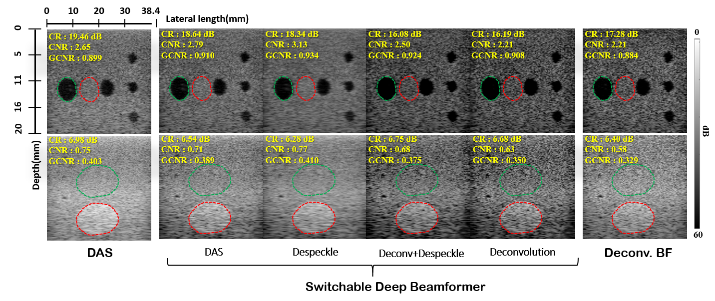
Figure 5: Reconstruction results of standard DAS-BF, Deconv.BF, and the proposed switchable deep beamformer for tissue mimicking phatom data from anechoic and hyperechoic regions.

V-A2 In-vivo test data

In Fig. 6, we compared two in-vivo examples scanned from the carotid and artery regions using $8.5$ MHz center frequency. Here again the proposed switchable deep beamformer achieves better performance compared to DAS and Deconv.BF methods especially in (Deconvolution/DeSpeckle) case which looks much sharper and have relatively less noise.

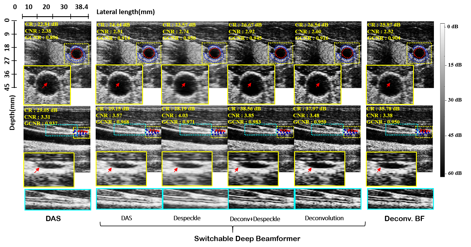
Figure 6: Reconstruction results of standard DAS-BF, Deconv.BF, and the proposed switchable deep beamformer for in-vivo scans from carotid and artery regions.

To further test the reconstruction quality of switchable deep beamformer, we showed four additional results in Fig. 7. From the figures it can be easily seen that the switchable deep beamformer can perform different tasks such as simple image formation, deconvolution, speckle suppression, and noise-suppressed deconvolution effectively.

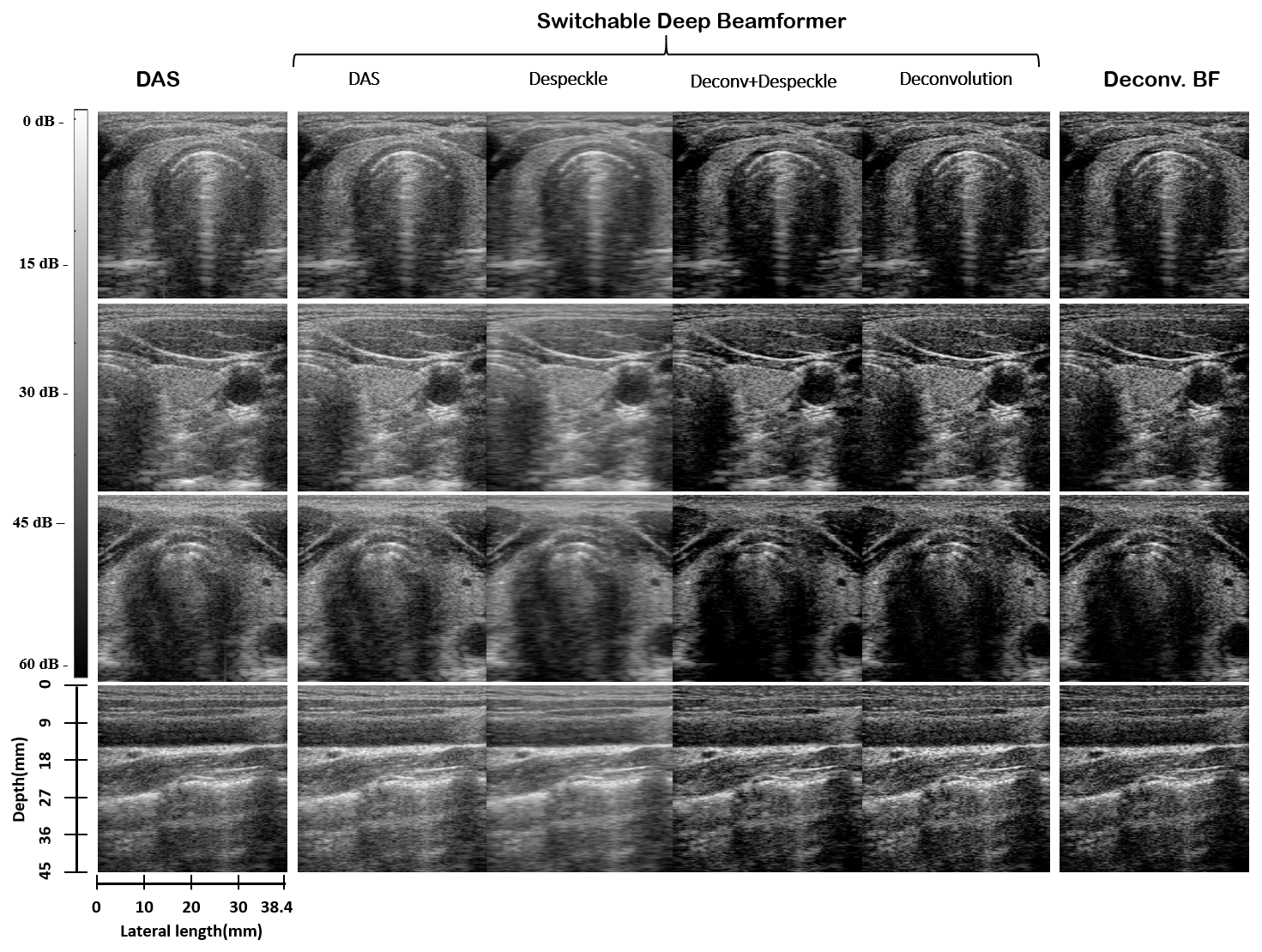
Figure 7: Reconstruction results of standard DAS-BF, Deconv.BF, and the proposed switchable deep beamformer for in-vivo scans from trachea, carotid, thyroid (central lobe), and artery region

V-A3 In-vivo independent data

In this experiment we used a dataset acquired from two completely different body parts scanned using $10$MHz operating frequency. In Fig. 8, we showed the results of two in vivo examples from calf and forearm regions. The images are generated using standard DAS, Deconv.BF, and the proposed switchable deep beamformer method. In Fig. 8, it can be easily seen that our method perform all four tasks effectively using a single model. In despeckle beamformer case, the switchable deep beamformer preserves the structural details while notably reduces the noise level. Interestingly, with combined deconvolution and despeckle, we can achieve two tasks (deblurring and denoising) tasks simultaneously.

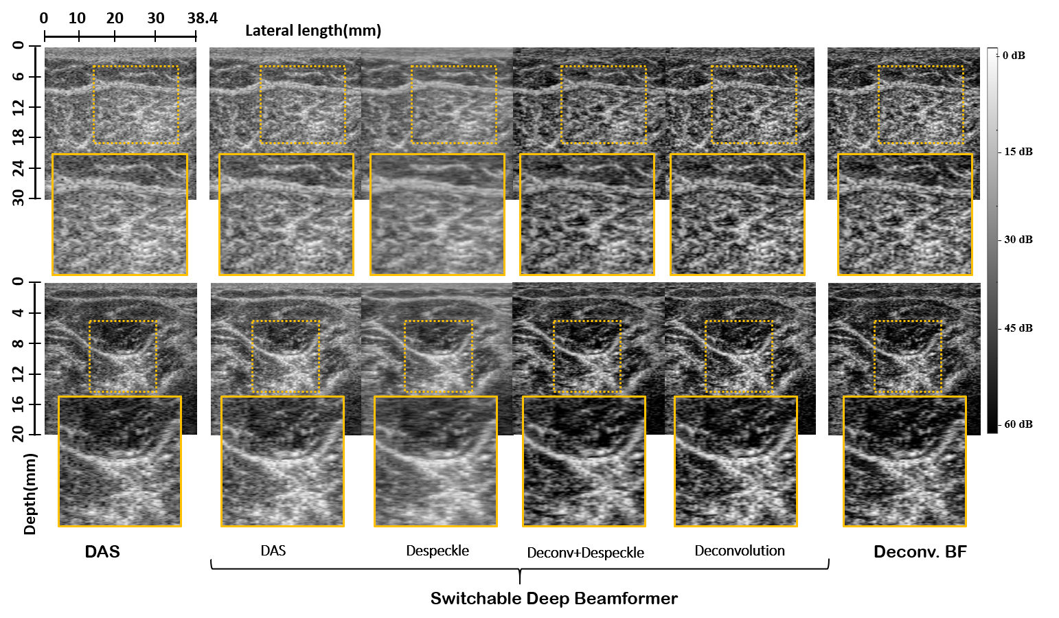
Figure 8: Reconstruction results of standard DAS-BF, Deconv.BF, and the proposed switchable deep beamformer for in-vivo scans from calf and forearm regions.

It is also noteworthy to point-out that the switchable deep beamformer was trained using only a subset of RF-data acquired from $8$ frames of a carotid/thyroid regions of a subject scanned with $8.5$MHz operating frequency. However, the performance in very diverse test scenarios is still remarkable, which clearly shows the generalization power of the proposed method.

V-B Quantitative comparison

To quantify the performance gain we compared the CR, CNR, and GCNR statistics of reconstructed B-mode images for all three datasets. Quantitatively CR, CNR, and GCNR values of switchable deep beamformer were slightly improved compared to the existing methods. Table I shows the comparison of DAS, Deconv.BF and proposed switchable deep beamformer method on all three dataset. In terms of CR, CNR and GCNR, the overall performance of switchable deep beamformer is remarkable. In carotid, thyroid, artery & trachea dataset, switchable deep beamformer for deconvolution produce highest CR among all while maintaining the noise level lower than the Deconv.BF. A similar trend can be seen in other dataset.

As expected the CNR and GCNR statistics of despeckle style switchable deep beamformer are highest as these measures are based on the sum of noise and background noise variance. Since despeckle style switchable beamformer effectively reduces the noise, it produces best statistics for noise based contrast measures. One interesting feature of the proposed method is its simultaneous deblurring and denoising capability. In Deconvolution+Despeckle mode, our method performs two competing tasks of deblurring and denoising, and surprisingly it enhances the CR statistics while maintaining the noise levels.

Interestingly, the proposed switchable beamformer also enhances the quality of B-mode images in DAS mode. In particular, for dataset $a$, $b$, and $c$ the GCNR values of proposed method in DAS mode are $0.02$, $0.011$, and $0.005$ units higher than the conventional DAS, respectively. Similarly, the deconvolution mode of switchable beamformer also outperform the Deconv.BF method. In particular, for dataset $a$ and $b$ it produced $0.016$, and $0.013$ units higher GCNR. While for dataset $c$ the results are quite comparable.

Since the encoder of the proposed switching beamformer was trained to produce a common representation for all types of target output, while the switching function was performed on decoder side, one possible reason for the enhanced performance would be that the network can learn better representation of the channel data through separate paths of forward and skip connections for contrast and speckle patterns, respectively. This may help the decoder to filter particular representation combination depending on the AdaIN encoded output.

TABLE I: Comparison of performance statistics with different beamformers

Beamforming		CR (dB)			CNR			GCNR
Method		a	b	c	a	b	c	a	b	c
DAS		18.53	16.97	24.92	2.29	2.17	2.63	0.824	0.785	0.923
Switchable DeepBF	(DAS)	18.81	15.77	24.71	2.45	2.30	2.63	0.844	0.796	0.928
	(Despeckle)	18.13	15.49	23.95	2.92	2.59	3.02	0.888	0.821	0.958
	(Deconvolution)	20.13	13.70	26.79	2.00	1.82	2.20	0.773	0.790	0.858
	(Deconvolution + Despeckle)	20.02	13.63	26.31	2.29	2.04	2.43	0.822	0.811	0.899
Deconv.BF		19.78	17.27	27.55	1.93	1.92	2.37	0.757	0.777	0.884

^a Test: carotid, thyroid, artery & trachea, ^b Test: tissue mimicking phantom, ^c Independent: calf & forearm

V-C Computational time

One big advantage of proposed switchable deep beamformer method is its reduced complexity, which allows for easily adaptation as only one model is used for various reconstruction tasks. This also allows fast reconstruction of ultrasound images with desired post processing filtration effects. The average reconstruction time for each depth planes is around $0.165$ (milliseconds), which is significantly lower than the conventional beamformer+filtration (deblurring/despeckle) methods. Interestingly, with combined learning of multiple tasks through AdaIN, the proposed model can achieve DAS and Deconv.BF like results with relatively shallower model compared to DeepBF which took around $4.8$ (milliseconds). The implementation method used in current study can be optimized by replacing the fully-connected neural network with fixed style vector values and optimized implementation for parallel reconstruction of multiple depth planes.

VI Conclusion

In this paper, we presented a novel switchable deep beamformer to generate desired quality B-mode ultrasound image directly from channel data with different post filtration effects by simply changing the AdaIN code. The proposed method is purely a data-driven method which harnesses the information in the spatio-temporal dimensions along the scan-line, axial depth and active channels measurement, which help in generating improved quality B-mode images compared to standard beamforming methods. In the proposed method, a single network was trained to produce four types of output including DAS, deconvolution, despeckle and deconvolution + despeckle directly from the channel data. The proposed method improved the contrast of B-modes images by preserving the dynamic range and structural details of the RF signal in both the phantom and in vivo scans, and can effectively perform computationally expensive post filtration task during the beamforming process. This post training adaptivity through AdaIN codes allow easily implementation; and therefore, this method can be an important platform for data-driven ultrasound beamformer.

References

- [1] F. Viola and W. F. Walker, “Adaptive signal processing in medical ultrasound beamforming,” in IEEE Ultrasonics Symposium, 2005., vol. 4, Sep. 2005, pp. 1980–1983.
- [2] J. Capon, “High-resolution frequency-wavenumber spectrum analysis,” Proceedings of the IEEE, vol. 57, no. 8, pp. 1408–1418, Aug 1969.
- [3] F. Vignon and M. R. Burcher, “Capon beamforming in medical ultrasound imaging with focused beams,” IEEE Transactions on Ultrasonics, Ferroelectrics, and Frequency Control, vol. 55, no. 3, pp. 619–628, March 2008.
- [4] K. Kim, S. Park, J. Kim, S. Park, and M. Bae, “A fast minimum variance beamforming method using principal component analysis,” IEEE Transactions on Ultrasonics, Ferroelectrics, and Frequency Control, vol. 61, no. 6, pp. 930–945, June 2014.
- [5] W. Chen, Y. Zhao, and J. Gao, “Improved capon beamforming algorithm by using inverse covariance matrix calculation,” in IET International Radar Conference 2013, April 2013, pp. 1–6.
- [6] C. . C. Nilsen and I. Hafizovic, “Beamspace adaptive beamforming for ultrasound imaging,” IEEE Transactions on Ultrasonics, Ferroelectrics, and Frequency Control, vol. 56, no. 10, pp. 2187–2197, October 2009.
- [7] A. M. Deylami and B. M. Asl, “A fast and robust beamspace adaptive beamformer for medical ultrasound imaging,” IEEE Transactions on Ultrasonics, Ferroelectrics, and Frequency Control, vol. 64, no. 6, pp. 947–958, June 2017.
- [8] A. C. Jensen and A. Austeng, “An approach to multibeam covariance matrices for adaptive beamforming in ultrasonography,” IEEE Transactions on Ultrasonics, Ferroelectrics, and Frequency Control, vol. 59, no. 6, pp. 1139–1148, June 2012.
- [9] ——, “The iterative adaptive approach in medical ultrasound imaging,” IEEE Transactions on Ultrasonics, Ferroelectrics, and Frequency Control, vol. 61, no. 10, pp. 1688–1697, Oct 2014.
- [10] K. H. Jin, Y. S. Han, and J. C. Ye, “Compressive dynamic aperture B-mode ultrasound imaging using annihilating filter-based low-rank interpolation,” in 2016 IEEE 13th International Symposium on Biomedical Imaging (ISBI). IEEE, 2016, pp. 1009–1012.
- [11] Y. H. Yoon, S. Khan, J. Huh, and J. C. Ye, “Efficient B-mode ultrasound image reconstruction from sub-sampled RF data using deep learning,” IEEE transactions on medical imaging, 2018.
- [12] A. Burshtein, M. Birk, T. Chernyakova, A. Eilam, A. Kempinski, and Y. C. Eldar, “Sub-Nyquist sampling and Fourier domain beamforming in volumetric ultrasound imaging,” IEEE Trans. Ultrason., Ferroelectr., Freq. Control, vol. 63, no. 5, pp. 703–716, 2016.
- [13] M. F. Schiffner and G. Schmitz, “Fast pulse-echo ultrasound imaging employing compressive sensing,” in Proc. IEEE Int. Ultrasonics Symposium (IUS), 2011, pp. 688–691.
- [14] A. C. Luchies and B. C. Byram, “Deep neural networks for ultrasound beamforming,” IEEE transactions on medical imaging, vol. 37, no. 9, pp. 2010–2021, 2018.
- [15] A. A. Nair, T. D. Tran, A. Reiter, and M. A. L. Bell, “A deep learning based alternative to beamforming ultrasound images,” in 2018 IEEE International Conference on Acoustics, Speech and Signal Processing (ICASSP). IEEE, 2018, pp. 3359–3363.
- [16] D. Hyun, L. L. Brickson, K. T. Looby, and J. J. Dahl, “Beamforming and speckle reduction using neural networks,” IEEE transactions on ultrasonics, ferroelectrics, and frequency control, vol. 66, no. 5, pp. 898–910, 2019.
- [17] S. Khan, J. Huh, and J. C. Ye, “Deep learning-based universal beamformer for ultrasound imaging,” in International Conference on Medical Image Computing and Computer-Assisted Intervention. Springer, Cham, 2019, pp. 619–627.
- [18] S. Khan, J. Huh, and J. C. Ye, “Adaptive and compressive beamforming using deep learning for medical ultrasound,” IEEE Transactions on Ultrasonics, Ferroelectrics, and Frequency Control, vol. 67, no. 8, pp. 1558–1572, 2020.
- [19] B. Luijten, R. Cohen, F. J. De Bruijn, H. A. Schmeitz, M. Mischi, Y. C. Eldar, and R. J. Van Sloun, “Adaptive ultrasound beamforming using deep learning,” IEEE Transactions on Medical Imaging, 2020.
- [20] X. Huang and S. Belongie, “Arbitrary style transfer in real-time with adaptive instance normalization,” in Proceedings of the IEEE International Conference on Computer Vision, 2017, pp. 1501–1510.
- [21] T. Karras, S. Laine, and T. Aila, “A style-based generator architecture for generative adversarial networks,” in Proceedings of the IEEE conference on computer vision and pattern recognition, 2019, pp. 4401–4410.
- [22] Y. Choi, Y. Uh, J. Yoo, and J.-W. Ha, “StarGAN v2: Diverse image synthesis for multiple domains,” in Proceedings of the IEEE/CVF Conference on Computer Vision and Pattern Recognition, 2020, pp. 8188–8197.
- [23] Y. Mroueh, “Wasserstein style transfer,” arXiv preprint arXiv:1905.12828, 2019.
- [24] G. Peyré, M. Cuturi et al., “Computational optimal transport: With applications to data science,” Foundations and Trends® in Machine Learning, vol. 11, no. 5-6, pp. 355–607, 2019.
- [25] C. Villani, Optimal transport: old and new. Springer Science & Business Media, 2008, vol. 338.
- [26] D. Ulyanov, A. Vedaldi, and V. Lempitsky, “Instance normalization: The missing ingredient for fast stylization,” arXiv preprint arXiv:1607.08022, 2016.
- [27] J. Duan, H. Zhong, B. Jing, S. Zhang, and M. Wan, “Increasing axial resolution of ultrasonic imaging with a joint sparse representation model,” IEEE Transactions on Ultrasonics, Ferroelectrics, and Frequency Control, vol. 63, no. 12, pp. 2045–2056, Dec 2016.
- [28] L. Zhu, C. Fu, M. S. Brown, and P. Heng, “A non-local low-rank framework for ultrasound speckle reduction,” in 2017 IEEE Conference on Computer Vision and Pattern Recognition (CVPR), July 2017, pp. 493–501.
- [29] D. Zhang, Y. Hu, J. Ye, X. Li, and X. He, “Matrix completion by truncated nuclear norm regularization,” in 2012 IEEE Conference on Computer Vision and Pattern Recognition. IEEE, 2012, pp. 2192–2199.
- [30] S. Gu, L. Zhang, W. Zuo, and X. Feng, “Weighted nuclear norm minimization with application to image denoising,” in Proceedings of the IEEE conference on computer vision and pattern recognition, 2014, pp. 2862–2869.
- [31] R. M. Rangayyan, Biomedical Image Analysis, ser. Biomedical Engineering, M. R. Neuman, Ed. Boca Raton, Florida: CRC Press, 2005.
- [32] A. Rodriguez-Molares, O. M. H. Rindal, J. D’hooge, S.-E. Måsøy, A. Austeng, M. A. L. Bell, and H. Torp, “The generalized contrast-to-noise ratio: a formal definition for lesion detectability,” IEEE Transactions on Ultrasonics, Ferroelectrics, and Frequency Control, vol. 67, no. 4, pp. 745–759, 2019.