Uplink Channel Estimation and Signal Extraction Against Malicious IRS in Massive MIMO System

Abstract

This paper investigates effect of malicious intelligence reflecting surface (IRS). The malicious IRS is utilized for performing attack by randomly reflecting data sequences of legitimate users (LUs) to a base station (BS). We find that the data sequences of LUs are correlative to the signals reflected by malicious IRS. The correlation undermines the performance of traditional eigenvalue decomposition (EVD)-based channel estimation (CE) methods. To address this challenge, we propose a empirical-distribution-based channel estimation approach in the presence of malicious IRS. The proposed method works by capturing desired convex hulls from signals disturbed by malicious IRS, on the basis of its empirical distribution. Simulation results show that our proposed approach outperforms traditional EVD-based methods as much as nearly 5 dB in normalized mean square error (NMSE).

I Introduction

Massive multiple-input and multiple-output (MIMO) is a key technology in fifth-generation (5G) communication that can achieve high speed and large capacity [1]. Its advantage depends on trustworthy channel state information (CSI) [2]. However, malicious users (MUs) may exist in 5G networks, and they may actively send interference to disturb channel estimation. As a result, trustworthy CSI cannot be obtained, and false CSI undermines the performance of a massive MIMO system. To obtain trustworthy CSI, it is important to investigate channel estimation under malicious attack [3].

Much work has investigated channel estimation under malicious attack. In[4], legitimate user (LU) and base station (BS) share a secret PS that is unknown to MU. The secret pilot sequence (PS) then enables channel estimation. In[5], all LUs and MUs select random PSs from a well-known pilot codebook that consists of orthogonal PSs. Based on the codebook, the BS firstly estimates the selected PSs, and then estimate channels. In[6], LUs and MUs independently send random symbols. Based on the independence, independent component analysis (ICA) could be invoked for channel estimation.

The above methods are implemented during the pilot phase. Other works estimate channels by employing eigenvalue decomposition (EVD) to signals received through the data phase. Based on the resulting eigenspaces, channels of LUs and MUs can be separated in probability as the number of antennas approaches infinity [7][8]. The transmission power gap between LUs and MUs is assumed and used for channel identification.

The works above assume that the MUs are equipped with traditional transmitters. On the other hand, intelligent reflecting surface (IRS), as a promising device, has attracted much attention. When signals propagate to IRS, the IRS could reflect the signals with programmable phase adjustment. By properly reflecting signals according to predesignated phase adjustment protocols, IRS could cooperate on channels estimation[9], or enlarging secrecy rate [10][11]. It is worth noting that IRS is only assumed to work as collaborator in prior works. However, to authors’ best knowledge, it is sparse to consider that IRS is used for attack.

In this paper, we consider malicious IRS. The IRS reflects pilot or data signals from LUs with unknown phase adjustment. The reflection signals propagate to BS, and interfere signal reception at the BS. Since the IRS is different with traditional active transmitters, existing methods based on active transmitter may be not applicable to combat malicious IRS [4, 5, 6, 7, 8]. To this problem, we propose a channel estimation and signal extraction method in the presence of malicious IRS.

The main contributions of the paper are as follows.

1. We find that there is correlation between the reflecting signal and the legitimate signal. And the correlation degrades the performance of traditional channel estimation methods based on EVD of the received signals[7][8].

2. To combat the attacks caused by the malicious IRSs, we use a geometric argument to develop signal extraction and channel estimation criteria. The geometric argument is robust to attack, but sensitive to noise. To optimize the proposed criteria, we presents an extractor to obtain geometric properties of desired signals from noisy observations. With the help of the extractor, we achieve signal extraction and channel estimation in the presence of attacks by solving two optimization problems.

Notation: Vectors are denoted by lowercase italicized letters, and matrices by uppercase italicized letters. A superscript $(\cdot)^{T}$ indicates a matrix transpose. We use tr(A) to denote the trace of matrix A, and $[\cdot]_{m}$ denotes the $m$th row of an input matrix or vector. $P_{X}$ denotes the stochastic distribution of the random variable $X$, $P_{X}(x)=\Pr(X=x)$. $P_{AB}$ denotes the joint distribution of random variables $A$ and $B$. $\odot$ denotes a dot product. $X\xrightarrow{a.s.}Y$ indicates that $X$ converges to $Y$ almost surely, where $X$ and $Y$ are generic random variables or bounded constants. $\left\|\cdot\right\|_{2}$ denotes the 2-norm.

II System Model

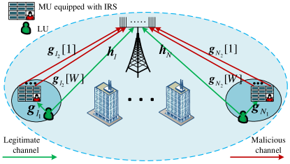
Figure 1: System model including one BS equipped with $M$ antennas and $N$ group users. Each MU is equipped with an IRS that includes $W$ elements. Through the pilot and data phases, the MUs reflect $W$ stream pilot sequences and interference sequences to the BS.

In Fig. 1, we consider system model including a BS equipped with $M$ antennas, $N$ single-antenna LUs, and $N$ MUs, where the $j$th LU is attacked by the $j$th MU, $j=1,2,\cdots,N$. Each MU is equipped with an IRS that includes $W$ elements. The uplink communication between the BS and the LUs takes place in the pilot and data phases, including $L_{p}$ and $n$ instants, respectively. The $j$th MU is assumed to locate close to the $j$th LU, and far away from other LUs. We thus assume that the $j$th MU conducts attack by only reflecting signals from the $j$th LU in the two phases. During the pilot phase, the IRSs of MUs reflect PSs without any phase-shift, and during the data phase, the MUs reflect information data sequences with random phase shift.

To be more precisely, in the pilot phase, the $j$th LU transmits PS $\emph{{x}}_{j}\in\mathbb{C}^{1\times L_{p}}$, which is selected from a public or secret pilot codebook X. The $j$th MU conducts pilot spoof attack, by using a identity matrix $\Phi_{p}=diag(1,\cdots,1)$, $\Phi_{p}\in\mathbb{C}^{W\times W}$, as reflection-coefficient matrix of its IRS. In this way, the MU reflects $\emph{{x}}_{j}$ without any phase adjustment. Then, the reflection signal is same to $\emph{{x}}_{j}$, which constitutes pilot spoof attack even the pilot codebook X is unknown to the MUs.

The received signals $\textbf{\emph{Y}}_{p}\in\mathbb{C}^{M\times L_{p}}$ in the pilot phase can be specified as

$$\footnotesize\textbf{\emph{Y}}_{p}= \footnotesize{\sum_{j=1}^{N}}(\emph{{h}}_{j}\emph{{x}}_{j}+\emph{{G}}_{j_{2}}\Phi_{p}\emph{{g}}_{j_{1}}\emph{{x}}_{j})+\textbf{\emph{N}}_{p}$$

$$= \footnotesize{\sum_{j=1}^{N}}(\emph{{h}}_{j}\emph{{x}}_{j}+{\sum_{w=1}^{W}}\emph{{g}}_{j_{w}}\emph{{x}}_{j})+\textbf{\emph{N}}_{p},$$ (1)

where $\emph{{h}}_{j}$ denotes the channel from the $j$th LU to the BS, $\emph{{h}}_{j}\in\mathbb{C}^{M\times 1}$; $\emph{{g}}_{j_{1}},\emph{{G}}_{j_{2}}$ respectively denote the channels from the $j$th LU to the $j$th MU and from the $j$th MU to the BS, $\emph{{g}}_{j_{1}}=[\emph{{g}}_{j_{1}}(1),\cdots,\emph{{g}}_{j_{1}}(W)]^{T}\in\mathbb{C}^{W\times 1}$, $\emph{{g}}_{j_{1}}(w)\in\mathbb{C}^{1\times 1}$, $\emph{{g}}_{j_{1}}(w)$ denotes the channel from the $j$th LU to the $w$th elememt of the $j$th MU. $\emph{{G}}_{j_{2}}=[\emph{{g}}_{j_{2}}[1],\cdots,\emph{{g}}_{j_{2}}[W]]\in\mathbb{C}^{M\times W}$, $\emph{{g}}_{j_{2}}[w]\in\mathbb{C}^{M\times 1}$, $\emph{{g}}_{j_{2}}[w]$ denotes the channel from the $w$th elements of $j$th MU to the BS; and $\emph{{g}}_{j_{w}}=\emph{{g}}_{j_{2}}[w]\emph{{g}}_{j_{1}}(w)$, denotes the cascaded channels of the $w$th element of IRS, $\emph{{g}}_{j_{w}}\in\mathbb{C}^{M\times 1}$. $\textbf{\emph{N}}_{p}\in\mathbb{C}^{M\times L_{p}}$ are Gaussian noise, and each element follows $\mathcal{CN}(0,\sigma^{2})$.

In the data phase, the $j$th LU transmits $\emph{{a}}_{j}\in\mathbb{C}^{1\times n}$. Due to the IRS of MU with $W$ reflection elements, the MU reflects $W$ stream signal sequences. We further define the diagonal matrix $\Phi_{j}(t)=diag(e^{\mathsf{i}\phi_{j_{1}}(t)},\cdots,e^{\mathsf{i}\phi_{j_{W}}(t)})$, $1\leq t\leq n$, $\Phi_{j}(t)\in\mathbb{C}^{W\times W}$ as the reflection-coefficient matrix of the $j$th IRS, which is randomly set according to $\Pr\{\phi_{j_{w}}(t)=0\}=p_{w}$, $\Pr\{\phi_{j_{w}}(t)=\pi\}=1-p_{w},1\leq w\leq W$. The received signals $\textbf{\emph{y}}(t)\in\mathbb{C}^{M\times 1}$ in the data phase can be specified as

$$\footnotesize\textbf{\emph{y}}(t) =\footnotesize{\sqrt{P}{\sum_{j=1}^{N}}(\emph{{h}}_{j}{\emph{{a}}_{j}}(t)+\emph{{G}}_{j_{2}}\Phi_{j}(t)\emph{{g}}_{j_{1}}{\emph{{a}}_{j}}(t))+\textbf{\emph{N}}}$$

$$=\footnotesize\sqrt{P}{\sum_{j=1}^{N}}(\emph{{h}}_{j}{\emph{{a}}_{j}}(t)+{\sum_{w=1}^{W}}\emph{{g}}_{j_{w}}{\emph{{b}}_{j_{w}}}(t))+\textbf{\emph{n}},1\leq t\leq n$$ (2)

$${\footnotesize\emph{{b}}_{j_{w}}}(t)={\emph{{a}}_{j}}(t)e^{\mathsf{i}\phi_{j_{w}}(t)},$$ (3)

$\emph{{b}}_{j_{w}}\in\mathbb{C}^{1\times n}$, where ${\emph{{a}}_{j}}(t),{\emph{{b}}_{j_{w}}}(t)$ respectively denote the $t$th elements in ${\emph{{a}}_{j}},{\emph{{b}}_{j_{w}}}$. $\textbf{\emph{n}}\in\mathbb{C}^{M\times 1}$ is Gaussian noise, and each element follows $\mathcal{CN}(0,\sigma^{2})$. $P$ is the transmission power.

Remark 1: Although we consider each LU to be attacked by single MU with $W$ elements, the model characterized by (II) and (3) is equivalent the two-MU with each having $\frac{W}{2}$ reflection elements. As such, our proposed technique is extensible for multi-MU model.

III Attack Strategies And Effects

III-A Attack strategies

The malicious IRS may perform deterministic and random reflection. These strategies are characterized by $p_{w}$. The deterministic reflection corresponds with $p_{w}=1$ or $p_{w}=0$. In other words, the IRSs reflect the signals of LUs with same or opposite phase. Then, the conventional EVD-based methods can be used to estimate composite channels ${\emph{{h}}_{j}}\pm{\sum_{w=1}^{W}}{\emph{{g}}_{j_{w}}}$, ${\emph{{a}}_{j}}$ could be decoded based on channel estimation.

The main challenge is brought by the random reflection, wherein $0<p_{w}<1$. The random reflection causes correlation between $\emph{{b}}_{j_{w}}$ and $\emph{{a}}_{j}$. To define this attack strategy mathematically, we assume that $\emph{{a}}_{j}$ is an independent and identically distributed (i.i.d.) sequence. According to (3), ${\emph{{b}}_{j_{w}}}$ is also an i.i.d. sequence. There are random variables $A$ and $B$ having the same stochastic distributions as each element of $\emph{{a}}_{j}$ and $\emph{{b}}_{j_{w}}$, respectively. Let us use $P_{A}$ and $P_{B}$ to denote stochastic distributions of $A$ and $B$, respectively. $\mathcal{A}_{j}$ and $\mathcal{B}_{j_{w}}$ are the alphabets of these two variables, $\mathsf{a}$ and $\mathsf{b}$ denote generic symbols of $\mathcal{A}_{j}$ and $\mathcal{B}_{j_{w}}$, respectively. When BPSK modulation is used by the LUs, it is not hard to obtain that $P_{A}(1)=P_{A}(-1)=\frac{1}{2}$, $P_{B|A}(1|1)=P_{B|A}(-1|-1)=p_{w}$, $P_{B|A}(-1|1)=P_{B|A}(1|-1)=1-p_{w}$. Therefore,

$$\footnotesize P_{A,B}(1,1)=\frac{1}{2}p_{w},P_{A}(1)P_{B}(1)=\frac{1}{4}.$$ (4)

By designing $p_{w}\neq\frac{1}{2}$ in (3), there exists

$$\footnotesize P_{A,B}({\mathsf{a},\mathsf{b}})\neq P_{A}({\mathsf{a}})P_{B}({\mathsf{b}}),\mathsf{a}\in\mathcal{A}_{j},\mathsf{b}\in\mathcal{B}_{j_{w}}.$$ (5)

Eq. (5) shows that ${\emph{{a}}_{j}}$ and ${\emph{{b}}_{j_{w}}}$ are correlative, and we refer the attack characterized by (5) as a correlative attack. We further find that the correlation coefficient between $\emph{{a}}_{j}$ and $\emph{{b}}_{jw}$ is given by $2p_{w}-1$. This indicates that the MU can control the strength of a correlative attack by adjusting its reflection probability $p_{w}$.

In summary, the MUs do not need to explicitly know $\emph{{a}}_{j}$. By setting $p_{w}\neq\frac{1}{2}$, correlative attack can be conducted. We proceed to analyze its effect below.

III-B Detriment of Correlative Attack

In the pilot phase, after receiving $\textbf{\emph{Y}}_{p}$, the BS may estimate channels of the LUs by projecting $\textbf{\emph{Y}}_{p}$ onto X,

$$\footnotesize\begin{split}&\left[\tilde{\emph{{h}}}_{1},\cdots,\tilde{\emph{{h}}}_{N}\right]=\textbf{\emph{Y}}_{p}\emph{{X}}^{H}\\ &=\left[{\emph{{h}}}_{1},\cdots,{\emph{{h}}}_{N}\right]+\left[{\emph{{g}}}_{1_{1}},\cdots,{\emph{{g}}}_{1_{W}},\cdots,{\emph{{g}}}_{N_{1}}\cdots,{\emph{{g}}}_{N_{W}}\right]+\textbf{\emph{N}}_{p}\emph{{X}}^{H},\end{split}$$ (6)

where the second equality relies on the orthogonal property of X. This indicates that the pilot spoof attack causes the channel estimation to combine the legitimate and malicious channels. There is a large estimation error. It is difficult to obtain trustworthy CSI only using $\textbf{\emph{Y}}_{p}$. We propose to use Y received during the data phase for channel estimation.

By collecting all the $\textbf{\emph{y}}(t)$, $1\leq t\leq n$ in a transmission block, the received signal in the data phase can be recast as

$$\footnotesize\textbf{\emph{Y}}=\textbf{\emph{C}}\textbf{\emph{S}}+\textbf{\emph{N}},$$ (7)

where $\footnotesize\textbf{\emph{C}}=\left[\textbf{\emph{H}},\textbf{\emph{G}}\right]$, $\footnotesize\textbf{\emph{S}}=\left[\begin{matrix}\textbf{\emph{A}},\textbf{\emph{B}}\end{matrix}\right]$, Y$=$$\left[\textbf{\emph{y}}(1),\textbf{\emph{y}}(2),\cdots,\textbf{\emph{y}}(n)\right]$,
$\footnotesize\textbf{\emph{H}}=[\emph{{h}}_{1},\emph{{h}}_{2},\cdots,\emph{{h}}_{N}]$, $\footnotesize{\textbf{\emph{A}}=\sqrt{P}\left[\begin{matrix}\emph{{a}}^{T}_{1},\emph{{a}}^{T}_{2},\cdots,\emph{{a}}^{T}_{N}\end{matrix}\right]^{T}}$,
G$=$$\left[{\emph{{g}}}_{1_{1}},\cdots,{\emph{{g}}}_{1_{W}},\cdots,{\emph{{g}}}_{N_{1}},\cdots,{\emph{{g}}}_{N_{W}}\right]$, $\footnotesize{\textbf{\emph{B}}=\sqrt{P}\left[\begin{matrix}\emph{{b}}^{T}_{1_{1}},\cdots,\emph{{b}}^{T}_{1_{W}},\cdots,\emph{{b}}^{T}_{{N_{1}}},\cdots,\emph{{b}}^{T}_{{N_{W}}}\end{matrix}\right]^{T}}$. $\footnotesize\textbf{\emph{Y}}\in\mathbb{C}^{M\times n}$, and each element in $\textbf{\emph{N}}\in\mathbb{C}^{M\times n}$ follows $\mathcal{CN}(0,\sigma^{2})$.

Traditional methods apply EVD to $\frac{1}{Mn}{\emph{{{Y}}}}{\emph{{{Y}}}}^{H}$. The resulting eigenspace is then used for jamming rejection when the jamming and legitimate data sequences are independent, i.e., $\frac{\emph{{{S}}}\emph{{{S}}}^{H}}{n}\xrightarrow{a.s.}{{\emph{{I}}_{N+WN}}}$. However, under correlative attacks, due to (5), we have $\frac{\emph{{{S}}}\emph{{{S}}}^{H}}{n}\xrightarrow{a.s.}R_{s}\in\mathbb{C}^{(N+WN)\times(N+WN)}$, where $R_{s}\neq{{\emph{{I}}_{N+WN}}}$. We find that a correlative attack undermines the performance of an EVD-based method using the received signal Y [7][8].

Proposition 1.

In a large-scale antenna regime, the right singular matrix of $\frac{1}{Mn}{\textbf{{Y}}}{\textbf{{Y}}}^{H}$ is $U_{\textbf{{Y}}}=\frac{1}{\sqrt{M}}[U_{W},\textbf{{C}}{{R}}^{-\frac{1}{2}}U_{s}]$, where $U_{W}\in\mathbb{C}^{M\times(M-N-WN)}$ has orthogonal columns and spans the null space of $[\textbf{{C}}{{R}}^{-\frac{1}{2}}U_{s}]$, $R\in\mathbb{C}^{(N+WN)\times(N+WN)}$ is a diagonal matrix depending on C, $U_{s}\in\mathbb{C}^{(N+WN)\times(N+WN)}$ is an orthogonal matrix, $\Lambda\in\mathbb{C}^{(N+WN)\times(N+WN)}$ is a diagonal matrix, and they are results of eigenvalue decomposition, i.e., $R^{\frac{1}{2}}R_{s}R^{\frac{1}{2}}=U_{s}\Lambda U^{H}_{s}$.

Proof.

Please refer to Appendix B for detailed proof. ∎

Remark 2: Notice that $U_{\emph{{{Y}}}}$ is determined by $\emph{{{C}}}{{R}}^{-\frac{1}{2}}$ and $U_{s}$. $U_{s}$ hinges on the degree of correlation among rows of S. In [7][8], all data streams are independent, i.e. , $U_{s}=\emph{{I}}$. Then $U_{\emph{{{Y}}}}$ is irrelevant to interference data. $U_{\emph{{{Y}}}}$ is thus used to directly eliminate interference from MUs. However, in this paper, due to correlative attacks, $U_{s}\neq\emph{{I}}$. The null space of MUs cannot be found from $U_{\emph{{{Y}}}}$, but the subspaces corresponding to MUs and LUs are united by $U_{\emph{{{Y}}}}$. This indicates that the MUs can directly manipulate $U_{\emph{{{Y}}}}$ by conducting a correlative attack, hence past work no longer applies [7][8].

As shown in (7), the received signals Y are mixtures of S, where the mixing matrix C includes all channel vectors. Every element of noise distortion N follows $\mathcal{CN}(0,\sigma^{2})$, $\textbf{\emph{N}}\in\mathbb{C}^{M\times n}$. This observation motivates us to achieve channel estimation by blind signal separation (BSS) approaches. Nevertheless, due to the attack, there is a correlation between $\emph{{a}}_{j}$ and $\emph{{b}}_{j_{w}}$, and the BS does not know the statistical characteristics of $\emph{{a}}_{j}$ and $\emph{{b}}_{j_{w}}$. Traditional BSS techniques[12][13] do not apply to the attack scenario considered in this paper. We next propose a BSS technique that works well under correlative attacks.

IV Signal Extraction and Channel Estimation

For a correlative attack, we consider a geometric argument that is insensitive to correlation. For instance, the convex hull of uCS [12], where u is the normalized vector combination vector of CS, only depends on the alphabet of uCS, regardless of the correlation of S. $\mathcal{L}\left({\emph{{u}}}\textbf{\emph{C}}\textbf{\emph{S}}\right)$ achieves its minimum when uCS includes only one data stream rather than the mixture of several streams, where $\mathcal{L}\left(\cdot\right)$ denotes the length of the convex hull of its input sequence, i.e., the convex perimeter [12]. Hence, the convex perimeter can be used for signal extraction, which is also the basis of channel estimation. However, the BS receives only the noisy observation of $\boldsymbol{CS}$, i.e., Y, rather than $\boldsymbol{CS}$ itself. The convex perimeter is very sensitive to noise. As seen in Fig. 2, the noise significantly changes the convex hull; hence, it impacts the convex perimeter. Proposition 2 provides an extractor capable of distilling alphabets from noisy observations.

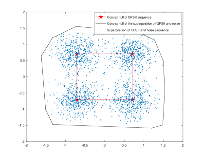
Figure 2: Illustration of the constellation of QPSK sequences (red dots) and QPSK and noise sequences (blue dots). Superimposed are the boundary and vertex of its convex hull; the noise changes the convex hull significantly.

Proposition 2.

Let us denote the alphabet of a discrete and $n$-length i.i.d. sequence $V^{n}$ as $\mathcal{V}$. Another noise sequence $W^{n}$ is independent of $V^{n}$. Then, from $V^{n}+W^{n}$, there exists an extractor $\mathbb{{F}}$, by whose use, i.e., $\mathbb{{F}}(V^{n}+W^{n})$, $\mathcal{V}$ can be extracted in probability as $n$ approaches infinity.

Proof.

Proposition 2 is proved by the proposal of extractor $\mathbb{{F}}$ in Appendix C.

∎

We use the extractor $\mathbb{{F}}$ to distill $\mathcal{V}$ from $V^{n}+W^{n}$. Since $V^{n}$ is a discrete sequence, the convex perimeter of $\mathcal{V}$ is equivalent to that of $V^{n}$. We thus have Corollary 1, which is based on Proposition 2.

Corollary 1.

For a discrete and $n$-length i.i.d. sequence $V^{n}$, there is another noise sequence $W^{n}$, which is independent of $V^{n}$. $\mathcal{L}\{\mathbb{F}\{V^{n}+W^{n}\}\}\rightarrow\mathcal{L}\{V^{n}\}$ in probability as n approaches infinity.

We next use $\mathbb{{F}}$ and $\mathcal{L}$ to extract signals and estimate channels.

IV-A Signal Extraction

Revisiting (7), Y is the superposition of CS and N. Notice that signal extraction corresponds to the minimization of the convex perimeter of uCS [12]. Relying on our proposed extractor $\mathbb{{F}}$ to achieve the convex perimeter, we establish an optimization problem subject to the signal extraction vector, where $\emph{{u}}\in\mathbb{C}^{1\times M}$,

$$\footnotesize\left[\hat{\emph{{u}}}\right] =arg\left\{\min\mathcal{L}\left\{\mathbb{F}\left\{\emph{{u}}\textbf{\emph{Y}}\right\}\right\}\right\}$$ (8)

$$s.t.\left\|\textbf{\emph{u}}\right\|_{2}=1.$$

Since $\emph{{u}}\textbf{\emph{Y}}=\emph{{u}}\textbf{\emph{C}}\textbf{\emph{S}}+\emph{{u}}\textbf{\emph{N}},$ according to Corollary 1, $\mathcal{L}\left\{\mathbb{F}\left\{\emph{{u}}\textbf{\emph{Y}}\right\}\right\}\rightarrow\mathcal{L}\{\emph{{u}}\textbf{\emph{C}}\textbf{\emph{S}}\}$ in probability as $n$ approaches infinity. The signal extraction vector is achieved by minimizing $\mathcal{L}\left\{\mathbb{F}\left\{\emph{{u}}\textbf{\emph{Y}}\right\}\right\}$ [12]. As the contrast function of (8) reduces the impact of noise, problem (8) can be solved by traditional gradient descent [12]. Details can be found in Algorithm 1.

The key difference of our work is the employment of $\mathbb{F}$ to reduce the impact of noise on the calculation of the convex perimeter. Previous work investigated the noiseless scenario, obtaining a signal extraction vector by minimizing the convex perimeter of uY [12]. In our model, due to the existence of noise, we propose $\mathbb{F}$ to obtain the convex perimeter of uCS. Simulations confirm that $\mathbb{F}$ significantly enhances extraction performance in the presence of a correlation attack and noise.

Based on (8), the signal of one user is extracted as

$$\emph{{s}}=\hat{\emph{{u}}}\textbf{\emph{Y}},$$ (9)

where $\emph{{s}}\in\mathbb{C}^{1\times n}$. We next estimate one channel corresponding to the extracted s.

IV-B Channel Estimation

Without loss of generality, we let $\emph{{c}}\in\mathbb{C}^{M\times 1}$ denote the channel corresponding to the extracted s. For $m=1\cdots M$, we let $[\cdot]_{m}$ denote the $m$th row of its input matrix or vector, and rewrite Y and R is the remainder signal.

$$[\textbf{\emph{Y}}]_{m}=[\textbf{\emph{R}}]_{m}+[\emph{{c}}]_{m}\emph{{s}}.$$ (10)

Both $[\textbf{\emph{R}}]_{m}$ and $[\emph{{c}}]_{m}\emph{{s}}$ are noisy observations that include noise and discrete sequences. Thus, $[\textbf{\emph{Y}}]_{m}$ is the noisy mixture of sequences corresponding to $[\textbf{\emph{R}}]_{m}$ and $[\emph{{c}}]_{m}\emph{{s}}$. $\mathcal{L}$ achieves its local minimum value when its input is the alphabet of a single signal rather than any mixture. Therefore, relying on $\mathbb{F}$, c can be estimated by

$$\small[\hat{\emph{{c}}}]_{m}=arg\left\{\min\mathcal{L}\left\{\mathbb{F}\left([\textbf{\emph{Y}}]_{m}-c^{\prime}\emph{{s}}\right)\right\}\right\},c^{\prime}\in\mathbb{C}.$$ (11)

To solve this problem, we also prove that the solution is in a finite and discrete set, which leads to an optimum solution when searching the finite and discrete set.

Proposition 3.

The optimum solution to (11) is included in a finite and discrete set, $\footnotesize{\mathrm{Q_{m}}=\left\{q\>|\>q=\frac{\mathsf{y}-\mathsf{y}^{\prime}}{\mathsf{z}-\mathsf{z}^{\prime}},\mathsf{z}\neq\mathsf{z}^{\prime},\mathsf{y}\neq\mathsf{y}^{\prime},\right.}$ $\left.\mathsf{y},\mathsf{y}^{\prime}\in\mathcal{Y}_{m},\mathsf{z},\mathsf{z}^{\prime}\in\mathcal{Z}\right\}$, where $\mathcal{Y}_{m}=\mathbb{F}\left\{[\textbf{{Y}}]_{m}\right\}$,$\mathcal{Z}=\mathbb{F}\left\{{\textbf{s}}\right\}$.

Proof.

Please refer to Appendix D for detailed proof. ∎

The key feature of (11) is the use of our proposed extractor $\mathbb{F}$ in the contrast function of (11), and in Proposition 3 to locate a solution. Previous work [14] only considers a noiseless scenario and implements no denoising measures.

Based on Proposition 3, we can estimate c as $\hat{\textbf{\emph{c}}}$ from (11). Then, with $\hat{\textbf{\emph{c}}}$ and the extracted c, the contribution of s can be removed from Y. After the deduction of $\hat{\textbf{\emph{c}}}\textbf{\emph{s}}$ from Y, let us repeat the signal extraction and channel estimation, as presented in Algorithm 1, until all channels are estimated.

In Algorithm 1, steps 3$\sim$12 solve the optimization problem (8) by gradient descent. The resulting vector $\hat{\emph{{u}}}$ is used for signal extraction in step 13. In steps 14$\sim$19, optimization problem (11) is solved by searching the discrete solution set given by Proposition 3. After s and $\hat{\textbf{\emph{c}}}$ are obtained, we deduct $\hat{\textbf{\emph{c}}}\textbf{\emph{s}}$ from Y, and iteratively run channel estimation.

% $i$: the $i$th signal extraction and channel estimation;

% $\mathbb{F}$: our proposed extractor given by Algorithm 2 in [Appendix C, [15]];

% $convhull$: the function of getting the convex points of its input sequence;

% $\mathbb{P}$: the function that finds $\emph{{u}}\textbf{\emph{Y}}(p_{1})$, $\emph{{u}}\textbf{\emph{Y}}(p_{2})$, $\emph{{u}}\textbf{\emph{Y}}(\cdots)$, and $\emph{{u}}\textbf{\emph{Y}}(p_{n^{\prime}})$ nearest to $\textbf{\emph{y}}(k_{1})$, $\textbf{\emph{y}}(k_{2})$, $\textbf{\emph{y}}(\cdots)$, and $\textbf{\emph{y}}(k_{n^{\prime}})$, respectively;

Input: Y, $N$, $W$, $M$

Output: signals $\textbf{\emph{s}}_{i}$ and channels $\hat{\textbf{\emph{c}}}_{i}$, for $i=1,2,\cdots,N_{L}+N_{M}$

1

2for $i=1:1:N+WN$ do

3       Initialization: $\emph{{u}}(1)=1$, $\emph{{u}}(2:M)=0$;

4       for iter=1:1:until $\mathcal{L}\left\{\mathbb{F}\left\{\emph{{u}}\textbf{\emph{Y}}\right\}\right\}$ minimum do

5             $\textbf{\emph{y}}=\mathbb{F}(\emph{{u}}\textbf{\emph{Y}})$ % y is the alphabet of uY 

6            $[k_{1},k_{2},\cdots,k_{n^{\prime}}]=convhull(\Re\left\{\textbf{\emph{y}}\right\},\Im\left\{\textbf{\emph{y}}\right\})$ 

7            $\mathcal{L}(\textbf{\emph{y}})=\sum_{i=2}^{n^{\prime}}\left\|\textbf{\emph{y}}(k_{i})-\textbf{\emph{y}}(k_{i-1})\right\|_{2}$ 

8            $[p_{1},p_{2},\cdots,p_{n^{\prime}}]=\mathbb{P}\left\{[k_{1},k_{2},\cdots,k_{n^{\prime}}]\right\}$  

9            $\emph{{Wp}}=\sum_{i=2}^{n^{\prime}}{\left\{\textbf{\emph{Y}}\left(:,p_{i}\right)-\textbf{\emph{Y}}\left(:,p_{i-1}\right)\right\}}$

10             $\quad\quad\quad{\left\{\textbf{\emph{Y}}\left(:,p_{i}\right)-\textbf{\emph{Y}}\left(:,p_{i-1}\right)\right\}^{H}}/(\left\|\textbf{\emph{y}}(k_{i})-\textbf{\emph{y}}(k_{i-1})\right\|_{2})$ 

11            $\emph{{g}}=({\frac{1}{2}\emph{{Wp}}{\emph{{u}}}-\emph{{u}}\mathcal{L}(\textbf{\emph{y}})})/{\left\|\emph{{{u}}}\right\|_{2}}$  

12            $\mu=1/({2{\left\|\emph{{g}}\right\|^{2}_{2}}}$)  

13            $\emph{{u}}=({\emph{{u}}-\mu\emph{{g}}})/{{\left\|\emph{{{u}}}-\mu\emph{{g}}\right\|_{2}}}$  

14       end for

15      

16      $\textbf{\emph{s}}_{i}=\hat{\emph{{u}}}\textbf{\emph{Y}}$ (9)  

17      $\mathcal{Z}_{i}=\mathbb{F}(\textbf{\emph{s}}_{i})$ 

18      for $m=1:1:M$ do

19             $\mathcal{Y}_{m}=\mathbb{F}([\emph{{Y}}]_{m})$  

20            $\mathrm{Q_{m}}=\big{\{}q\>|\>q=\frac{\mathsf{y}-\mathsf{y}^{\prime}}{\mathsf{z}-\mathsf{z}^{\prime}},\mathsf{z}\neq\mathsf{z}^{\prime},\mathsf{y}\neq\mathsf{y}^{\prime},\mathsf{y},\mathsf{y}^{\prime}\in\mathcal{Y}_{m},\mathsf{z},\mathsf{z}^{\prime}\in\mathcal{Z}_{i}\big{\}}$  

21            $[\hat{\textbf{\emph{c}}}_{i}]_{m}=arg\left\{\min\mathcal{L}\left\{\mathbb{F}([\textbf{\emph{Y}}]_{m}-c^{\prime}\textbf{\emph{s}}_{i})\right\}\right\}$, $c^{\prime}\in\mathrm{Q_{m}}$ (8)  

22       end for

23      $\textbf{\emph{Y}}=\textbf{\emph{Y}}-\hat{\textbf{\emph{c}}}_{i}{\textbf{\emph{s}}_{i}}$

24 end for

Algorithm 1 Signal Extraction and Channel Estimation

IV-C Channel Identification

Note that the proposed signal extraction depends on the minimum of $\mathcal{L}\left\{\mathbb{F}\left\{\emph{{u}}\textbf{\emph{Y}}\right\}\right\}$, where $\mathcal{L}\left\{\mathbb{F}\left\{\emph{{u}}\textbf{\emph{Y}}\right\}\right\}$ remains unchanged when the angles of its input are rotated. Optimization problem (8) just indicates that the extracted signal belongs to one user, but it cannot determine which user corresponds to the extracted signal. Hence, order ambiguity exists.

Such ambiguities widely exist in BSS-based work [12] [16]. Previous work [16] assumes that the phase and order ambiguities are resolved perfectly by outdated estimate results. We similarly assume perfect channel identification.

V experimental results

As the system model shows, there are $N$ group users, each group includes one LU and one MU, and each MU is equipped with an IRS with $W$ elements that can randomly reflect $W$ stream signal sequences. The channel is i.i.d. Rayleigh fading, with an $M\times(N+WN)$ channel matrix. Without loss of generality, we consider a massive MIMO system with $M=128$ antennas, and attack scenarios of $N=2$, $W=2$, $N=1$, $W=3$ and $N=1$, $W=1$, as shown in Figs. 3, 4, and 5, respectively. The independent symbols of LUs are drawn from a BPSK constellation, and we assume that the MUs conduct the attack according to (3). When $W=1$, we set $\Pr\{\phi_{j_{1}}=0\}=0.8$, and then the correlation coefficient of $\emph{{a}}_{j}$ and $\emph{{b}}_{j_{1}}$ is $0.6$. When $W=2$, we set $\Pr\{\phi_{j_{1}}=0\}=0.6$, $\Pr\{\phi_{j_{2}}=0\}=0.7$. Then the correlation coefficients of $\emph{{a}}_{j}$ and $\emph{{b}}_{j_{1}}$ and of $\emph{{a}}_{j}$ and $\emph{{b}}_{j_{2}}$ are $0.2$ and $0.4$, respectively. When $W=3$, we set $\Pr\{\phi_{j_{1}}=0\}=0.6$, $\Pr\{\phi_{j_{2}}=0\}=0.7$, $\Pr\{\phi_{j_{3}}=0\}=0.8$. Then the correlation coefficients of $\emph{{a}}_{j}$ and $\emph{{b}}_{j_{1}}$, $\emph{{a}}_{j}$ and $\emph{{b}}_{j_{2}}$, and $\emph{{a}}_{j}$ and $\emph{{b}}_{j_{3}}$ are $0.2$, $0.4$, and $0.6$, respectively. The BS estimates channels and achieves CSI. According to the achieved CSI, BS uses zero forcing (ZF) detection to get the signal-to-interference-and-noise ratio (SINR) of all users. The normalized mean square error (NMSE) of the channel estimation and the bit error rate (BER) of the separation signal are also selected as performance metrics. We simulate and compare the performance of our proposed method and those based on bounded component analysis (BCA) [12] and EVD [7]. We also simulate the performance achieved under perfect CSI. Since we consider multiple users, to evaluate the performance of every user, we use the mean-SINR, min-SINR, max-NMSE, mean-NMSE, and min-NMSE, where “mean”, “min”, and “max” represent the average, worst, and best performance metrics over all users.

Because the EVD-based method depends on the transmission power gap between LUs and MUs to get the separability of eigenspaces, we set the path-losses of MUs less than LUs, that means the interference of MUs in our proposed method is much stronger than that of EVD-based method. We use EVD-0.3 and EVD-0.5 denote the path-losses of MUs are 0.3 and 0.5, respectively.

In Figs. 3, 4, and 5, the path loss of MUs in the proposed method is $1$. Although the interference of MUs in our proposed method was greater than the EVD-based method, the proposed method performs better than the EVD-based method, and our method performs close to the perfect CSI. Specifically, it is observed in Figs. 3, 4, and 5 that as the the correlation coefficient is fixed, the performance of the EVD-based method remains almost unchanged despite an increase in the signal-to-noise ratio (SNR). In contrast, in Fig. 6, we consider $N=1,W=1$, and the performance of the EVD-based method changes significantly when the correlation coefficient of $\emph{{a}}_{j}$ and $\emph{{b}}_{j_{1}}$ increases from $0$ to $0.8$. Fig. 6 presents the performance of $N=1$ and $W=1$ under varying correlation coefficients with an SNR of 16 dB. The proposed method has better performance than the EVD-based method with different correlation coefficients. This is consistent with Proposition 1, indicating that in the presence of a correlative attack, the signals of LUs and MUs no longer lie in distinct eigenspaces of the received signal matrix in the BS. Instead, the subspace of the attack signals overlaps with the eigenspace corresponding to the LUs, thus leading to attack leakage when the EVD-based method employs eigenvectors corresponding to the LUs for the received signal projection.

In our proposed method, we consider reducing the impact of noise and use geometric properties to overcome the impact of a correlative attack. The performance increases as the SNR increases in Figs. 3, 4, and 5, and is unchanged in a certain range as the correlation coefficient increases in Fig. 6. Specifically, in Fig. 6, it is observed that when the correlation coefficient is $0.6$, the SINR of the proposed method is better than that of the EVD-based method by more than $5$ dB. The EVD-based method has better performance when the pass losses of MUs are less. This indicates that the stronger the attack signals, the worse the performance is of the EVD-based method. This could be because the EVD-based method attempts to eliminate attack signals as interference. The proposed method treats attack signals as those of regular users, rather than interference. We also estimate attack signals and channels instead of eliminating them as interference. Thus the proposed method outperforms the EVD-based method under much stronger attacks.

Next, in Figs. 3, 4, and 5, we present the performance of the BCA method, and we see that the proposed method performs much better. For instance, it is observed in Fig. 3 that the mean-SINR and min-SINR of the proposed method are better than those of the BCA method by more than $5$ dB. The NMSE of the proposed method is better than that of the BCA method, especially at low SNRs.

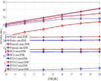
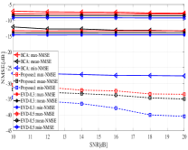
Figure 3: (a) SINR and (b) NMSE of proposed, BCA, and EVD-based methods versus SNR with $N=2$, $W=2$. The correlation between signal sequences of LU and MU are fixed at $0.2$ and $0.4$, respectively.

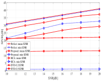
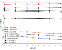
Figure 4: (a) SINR and (b) NMSE of proposed, BCA, and EVD-based methods versus SNR with $N=1$, $W=3$. The correlation between signal sequences of LU and MU are fixed at $0.6$, $0.7$ and $0.8$.

To study the influence of signal correlation on performance, in  Fig. 6, it is observed that the mean-SINR and min-SINR of our proposed method outperform the BCA method by more than $5$ dB, and the NMSE of the proposed method outperforms that of the BCA method. Fig. 7 shows the BER performance of $N=2$, $W=2$; $N=1$, $W=3$; $N=1$, $W=1$ for the proposed method and BCA method. Fig. 7 shows the performance of $N=1$, $W=1$ with different correlation coefficients. The proposed method outperforms the BCA method in any case.

We further discover that the performance of both methods, especially the BCA method, will deteriorate as the correlation coefficient increases. Actually, the BCA method works well in a noiseless scenario. This indicates that the BCA method is sensitive to noise, because it is based on geometric properties of desired signals. The existence of noise changes the shape of the convex hull of desired signals. Consequently, geometric properties cannot be captured exactly in the presence of noise. Therefore, the existence of Gaussian noise damages the performance of the BCA method against a dependence attack. In contrast, the performance of our proposed method changes little as the correlation of users’ symbols increases. Our method considers the reduction of the impact of noise, as mentioned above, thus correlation does not significantly degrade its performance.

In summary, based on our simulation results, the proposed method outperforms the BCA and EVD-based methods in the sense of SINR, NMSE, and BER.

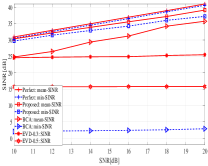
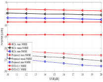
Figure 5: (a) SINR and (b) NMSE of proposed, BCA, and EVD-based methods versus SNR with $N=1$, $W=1$. The correlation between LU and MU is fixed at $0.6$.

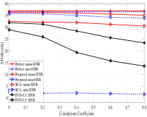
Figure 6: (a) SINR and (b) NMSE of proposed, BCA, and EVD-based methods versus correlation coefficient with $N=1$, $W=1$. The SNR is fixed at 16 dB.

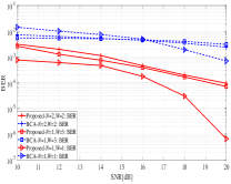
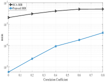
Figure 7: BER of proposed and BCA methods: (a) $N=2$, $W=2$; $N=1$, $W=3$; $N=1$, $W=1$. (b) $N=1$, $W=1$. The SNR is fixed at 16 dB.

VI conclusion

Above all, we focus on channel estimation under a correlative attack with noise. We propose an extractor $\mathbb{F}$ that can distill alphabets from a noisy signal. We apply this extractor to signal extraction and channel estimation. Numerical results show that the proposed method performs better than the BCA and EVD-based methods under a correlative attack in a noisy environment.

Appendix A Proof of correlation coefficient

When BPSK modulation is used by the signal sequence $\emph{{a}}\in\mathbb{C}^{1\times n}$, it is not hard to obtain that $P_{A}(1)=P_{A}(-1)=\frac{1}{2}$. $P_{A}$ denotes the stochastic distribution of a. Due to the IRS, $1\leq t\leq n$, and

$$\emph{{b}}(t)=\emph{{a}}(t)e^{\mathsf{i}\phi},$$ (12)

where $\phi$ denotes the reflection phase of the IRS. It is randomly set according to $\Pr\{\phi=0\}=p$, $\Pr\{\phi=\pi\}=1-p$. ${\emph{{a}}}(t),{\emph{{b}}}(t)$ are the respective $t$th elements in ${\emph{{a}}},{\emph{{b}}}$. Then the transition probability $P_{B|A}({1}|{1})=P_{B|A}({-1}|-1)=p$, $P_{B|A}({-1}|{1})=P_{B|A}({1}|{-1})=1-p$. Then in b,

$$P_{B}(1) =P_{A}(1)P_{B|A}({1}|{1})+P_{A}(-1)P_{B|A}({1}|{-1})$$ (13)

$$=\frac{1}{2}p+\frac{1}{2}(1-p)=\frac{1}{2}.$$

$$P_{B}(-1) =1-P_{B}(1)=\frac{1}{2}.$$ (14)

$P_{B}$ denotes the stochastic distribution of b. $\overline{\emph{{a}}}$ and $\overline{\emph{{b}}}$ are $0$ as $n$ approaches infinity, $\overline{(\cdot)}$ denotes the mean value of its input sequence. Then the correlation coefficient of a and b is

$$\rho_{{\emph{{a}}}{\emph{{b}}}} =\frac{\sum_{t=1}^{n}(\emph{{a}}(t)-\overline{\emph{{a}}})(\emph{{b}}(t)-\overline{\emph{{b}}})}{\sqrt{\sum_{t=1}^{n}(\emph{{a}}(t)-\overline{\emph{{a}}})^{2}}\sqrt{\sum_{t=1}^{n}(\emph{{b}}(t)-\overline{\emph{{b}}})^{2}}}$$ (15)

$$=\frac{\sum_{t=1}^{n}\emph{{a}}(t)\emph{{b}}(t)}{\sqrt{\sum_{t=1}^{n}\emph{{a}}(t)^{2}}\sqrt{\sum_{t=1}^{n}\emph{{b}}(t)^{2}}}=\frac{pn-(1-p)n}{n}$$

$$=2p-1.$$

Appendix B Proof of Proposition 1

According to [[17], Corollary 1], we obtain $\frac{1}{M}\textbf{\emph{H}}^{H}\textbf{\emph{H}}\xrightarrow{a.s.}\frac{1}{M}{\rm{Tr(R_{H})}},\frac{1}{M}\textbf{\emph{G}}^{H}\textbf{\emph{G}}\xrightarrow{a.s.}\frac{1}{M}{\rm{Tr(R_{G})}},\frac{1}{M}\textbf{\emph{G}}^{H}\textbf{\emph{H}}\xrightarrow{a.s.}0,\frac{1}{M}\textbf{\emph{H}}^{H}\textbf{\emph{G}}\xrightarrow{a.s.}0$. Then we have $\frac{1}{M}\textbf{\emph{C}}^{H}\textbf{\emph{C}}\xrightarrow{a.s.}\frac{1}{M}\left[\begin{matrix}\rm{Tr(R_{H})}&0\\ 0&\rm{Tr(R_{G})}\end{matrix}\right]=R$, and $U^{H}_{\textbf{\emph{Y}}}U_{\textbf{\emph{Y}}}\xrightarrow{a.s.}\emph{{I}}_{M}$, and we have $\frac{\textbf{\emph{S}}\textbf{\emph{S}}^{H}}{n}\xrightarrow{a.s.}{{R_{s}}}$. Then we decompose $R_{\emph{{{Y}}}}$ as

$$R_{\emph{{{Y}}}} =\frac{1}{M}{\textbf{\emph{C}}}R_{s}\textbf{\emph{C}}^{H}+\frac{\sigma^{2}}{M}\emph{{I}}_{M}$$ (16)

$$=\frac{1}{M}\textbf{\emph{C}}R^{-\frac{1}{2}}R^{\frac{1}{2}}R_{s}R^{\frac{1}{2}}R^{-\frac{1}{2}}\textbf{\emph{C}}^{H}+\frac{\sigma^{2}}{M}\emph{{I}}_{M}$$

$$\overset{(a)}{=}\frac{1}{M}\textbf{\emph{C}}R^{-\frac{1}{2}}U_{s}\Lambda U^{H}_{s}R^{-\frac{1}{2}}\textbf{\emph{C}}^{H}+\frac{\sigma^{2}}{M}\emph{{I}}_{M}$$

$$\xrightarrow{a.s.}\frac{1}{M}\textbf{\emph{C}}R^{-\frac{1}{2}}U_{s}\Lambda U^{H}_{s}R^{-\frac{1}{2}}\textbf{\emph{C}}^{H}+\frac{\sigma^{2}}{M}U_{\emph{{{Y}}}}U^{H}_{\emph{{{Y}}}}$$

$$=\frac{1}{M}\textbf{\emph{C}}R^{-\frac{1}{2}}U_{s}\Lambda U^{H}_{s}R^{-\frac{1}{2}}\textbf{\emph{C}}^{H}+\frac{\sigma^{2}}{M}U_{W}U^{H}_{W}+$$

$$\frac{\sigma^{2}}{M}\textbf{\emph{C}}R^{-\frac{1}{2}}U_{s}U^{H}_{s}R^{-\frac{1}{2}}\textbf{\emph{C}}^{H}$$

$$=U_{\textbf{\emph{Y}}}diag\{\sigma^{2}\textbf{I}_{M-N-WN},\Lambda+\sigma^{2}\textbf{I}_{N+WN}\}U^{H}_{\textbf{\emph{Y}}}.$$

As long as $n$ is sufficiently large, $R_{\emph{{{Y}}}}$ can be approached by $\frac{1}{Mn}\emph{{{Y}}}\emph{{{Y}}}^{H}$. The convergence follows $U_{\textbf{\emph{Y}}}U^{H}_{\textbf{\emph{Y}}}\xrightarrow{a.s.}\emph{{I}}_{M}$, and the equation ($a$) follows $R^{\frac{1}{2}}R_{s}R^{\frac{1}{2}}=U_{s}\Lambda U^{H}_{s}$.

Appendix C Proof of Proposition 2

Due to space limitations, we sketch the proof of Proposition 2 and present an algorithm to implement it. We use $L^{n}$ to denote $V^{n}+Q^{n}$. Note that $L^{n}$, $V^{n}$, $Q^{n}$ are i.i.d. random sequences. Let $V$ denote a generic random variable with the same stochastic distribution as each element of $V^{n}$. Similarly, we use generic random variables $Q$ and $L$ following stochastic distributions identical to those of elements of $Q^{n}$ and $L^{n}$, respectively. Furthermore, note that $Q^{n}$ and $V^{n}$ are independent of each other. As a consequence, $W$ is independent of $V$. Since $L^{n}=V^{n}+Q^{n}$, we specify $L$ by $L=V+Q$. Let $F_{{L}}$, $F_{{V}}$, and $F_{Q}$ denote the distributions of $L$, $V$, and $Q$, respectively. Then, because $V$ and $Q$ are independent of each other, we have

$$\Phi_{F_{L}}(\boldsymbol{f})=\Phi_{F_{V}}(\boldsymbol{f})\Phi_{F_{Q}}(\boldsymbol{f}),$$ (17)

where $\Phi_{F}(\boldsymbol{f})$ denotes the characteristic function (CF) of the distribution $F$, and $\boldsymbol{f}$ is the frequency vector. Note that the noise variance parameter $\sigma_{Q}^{2}$ is a characteristic of the receiver circuitry and can be measured a priori. We may assume that its value is known; hence, $\Phi_{F_{Q}}(\boldsymbol{f})=\exp\left\{-2{\sigma_{Q}^{2}}\pi^{2}\left|\boldsymbol{f}\right|^{2}\right\}$ is also known. Therefore, according to (17), $F_{V}$ is achieved by

$$F_{V}=\Phi^{-1}\left(\frac{\Phi_{F_{L}}(\boldsymbol{f})}{\exp\left\{-2{\sigma_{Q}^{2}}\pi^{2}\left|\boldsymbol{f}\right|^{2}\right\}}\right),$$ (18)

where $\Phi^{-1}\left(\cdot\right)$ denotes the inverse CF of its input. It is worth noting that in (18), $F_{V}$ is perfectly obtained from $L$, even though $L$ includes noise $Q$ with arbitrary average power $\sigma_{Q}^{2}$. $V$ has a discrete alphabet $\mathcal{V}$ that can be achieved by finding points $\mathsf{v}$ that make $F_{V}\left(\mathsf{v}\right)>0$. As a result, the extractor given by (18) satisfies our goal of extracting alphabets from noisy observations. However, in practice, to implement (18) is a challenge for two reasons.

1. Due to attack, $F_{L}$ is unknown. The lack of $F_{L}$ leads the inability to obtain $\Phi_{F_{L}}(\boldsymbol{\omega})$ exactly.

2. $\Phi\left(\cdot\right)$ and $\Phi^{-1}\left(\cdot\right)$ correspond to a continuous Fourier transform (CFT) and inverse CFT, respectively. The transforms over a continuous domain may give rise to issues of implementation.

Motivated by these two challenges, we propose an extractor according to (18) by using a quantized empirical distribution of $L^{n}$ to approach $F_{L}$ according to the law of large numbers (LLN), and using a discrete Fourier transform (DFT) and inverse DFT to approach $\Phi\left(\cdot\right)$ and $\Phi^{-1}\left(\cdot\right)$, respectively. According to LLN and the Nyquist sampling theorem, the approximation of $\Phi_{F_{L}}(\boldsymbol{f})$ becomes more accurate as the quantization level and number of observations increase. In this sense, on the basis of (18), Proposition 2 has been proved. Furthermore, we provide an algorithm to implement (18) by sequential quadratic programming (SQP). To be more precise, notice that (18) is equivalent to

$$F_{V}\left(v\right)=\underset{\hat{F}_{V}}{\arg\min}\iint\left|\Phi_{F_{L}}(\boldsymbol{f})-\Phi_{\hat{F}_{V}}(\boldsymbol{f})\Phi_{F_{Q}}(\boldsymbol{f})\right|^{2}d\boldsymbol{f},$$ (19)

where $\hat{F}_{V}$ is a stochastic distribution function. To approximate $\Phi_{F_{L}}(\boldsymbol{f})$, we quantize $L$ and achieve an empirical distribution,

$$\varPi_{\widehat{L}^{n}}\left(n_{1},n_{2}\right)=\frac{1}{n}\sum_{i=1}^{n}\mathtt{1}\left\{\Re\left\{L_{i}\right\}\in\mathcal{B}\left(n_{1}\right)\right\}\mathtt{1}\left\{\Im\left\{L_{i}\right\}\in\mathcal{B}\left(n_{2}\right)\right\},$$ (20)

where $L_{i}$ is the $i$-th variable of $L^{n}$; $\Re\left\{\cdot\right\}$ and $\Im\left\{\cdot\right\}$ denote the real and imaginary parts, respectively, of its input; and $\mathtt{1}\left\{\cdot\right\}$ is an indicator function. $\mathcal{B}\left(n_{1}\right)=\left[-d_{1}+n_{1}\triangle,-d_{1}+\left(n_{1}+1\right)\triangle\right]$, $\triangle=\frac{2d_{1}}{n_{1}}$, $d_{1}=\sqrt{n_{1}}$. For $\boldsymbol{f}=\left[f_{r},\>f_{i}\right]$, $\Phi_{F_{L}}(\boldsymbol{f})$ could be approached by

$$\Phi_{F_{L}}(\boldsymbol{f})=\int F_{L}\left({l}\right)\exp\left\{-\mathsf{i}2\pi\boldsymbol{f}\left[\begin{array}[]{c}\Re\left({l}\right)\\ \Im\left({l}\right)\end{array}\right]\right\}d{l}$$ (23)

$$\overset{N,n\rightarrow\infty}{\rightarrow}\triangle^{2}\exp\left\{\mathsf{i}2\pi\left(f_{r}+f_{i}\right)d_{1}\right\}$$

$$\times\sum_{n_{1}=1}^{N}\sum_{n_{2}=1}^{N}\varPi_{\widehat{L}^{n}}\left(n_{1},n_{2}\right)\exp\left\{-\mathsf{i}2\pi n_{1}\triangle f_{r}\right\}\exp\left\{-\mathsf{i}2\pi n_{2}\triangle f_{i}\right\}.$$

Sampling $\Phi_{F_{L}}(\boldsymbol{f})$ across $\left(k_{1}f,\>k_{2}f\right)$, $k_{1},k_{2}=1,\ldots,N_{f}$, $f=\frac{1}{\triangle N_{f}}$, we have

$$\Phi_{F_{L}}(k_{1}f,\>k_{2}f)\overset{N,n\rightarrow\infty}{\rightarrow}\tilde{\Phi}_{F_{L}}(k_{1}f,\>k_{2}f)$$

$$=\triangle^{2}\exp\left\{\mathsf{i}2\pi\left(\frac{k_{1}}{\triangle N_{f}}+\frac{k_{2}}{\triangle N_{f}}\right)d_{1}\right\}$$

$$\times\underbrace{\sum_{n_{1}=1}^{N}\sum_{n_{2}=1}^{N}\varPi_{\widehat{L}^{n}}\left(n_{1},n_{2}\right)\exp\left\{-\mathsf{i}2\pi\frac{n_{1}k_{1}}{N_{f}}\right\}\exp\left\{-\mathsf{i}2\pi\frac{n_{2}k_{1}}{N_{f}}\right\}}_{\left[\mathbb{DFT}\left\{\varPi_{\widehat{L}^{n}}\right\}\right]_{k_{1},k_{2}}},$$

where $\tilde{\Phi}_{F_{L}}(k_{1}f,\>k_{2}f)$ can be obtained from the DFT of $\varPi_{\widehat{L}^{n}}$, denoted by $\mathbb{DFT}\left\{\varPi_{\widehat{L}^{n}}\right\}$, which is an $N_{f}\times N_{f}$ matrix whose $(k_{1},k_{2})$-th element corresponds to the value of $\mathbb{DFT}\left\{\varPi_{\widehat{L}^{n}}\right\}$ in the $(k_{1},k_{2})$-th frequency. Hence, we approximate $\Phi_{F_{L}}(\boldsymbol{f})$ by an $N_{f}\times N_{f}$ matrix $\mathbf{L}$ whose $(k_{1},k_{2})$-th element is

$$\left[\mathbf{L}\right]_{k_{1},k_{2}}=\triangle^{2}\exp\left\{\mathsf{i}2\pi\left(\frac{k_{1}}{\triangle N_{f}}+\frac{k_{2}}{\triangle N_{f}}\right)d_{1}\right\}\left[\mathbb{DFT}\left\{\varPi_{\widehat{L}^{n}}\right\}\right]_{k_{1},k_{2}}.$$ (24)

Similarly, $\Phi_{{F}_{V}}(\boldsymbol{f})$ can be approximated by an $N_{f}\times N_{f}$ matrix $\mathbf{V}$ whose $(k_{1},k_{2})$-th element is

$$\left[\mathbf{V}\right]_{k_{1},k_{2}}=\triangle^{2}\exp\left\{\mathsf{i}2\pi\left(\frac{k_{1}}{\triangle N_{f}}+\frac{k_{2}}{\triangle N_{f}}\right)d_{1}\right\}\left[\mathbb{DFT}\left\{\varPi_{\widehat{V}^{n}}\right\}\right]_{k_{1},k_{2}}.$$ (25)

$\varPi_{\widehat{V}^{n}}$ is the empirical distribution of the quantized sequence of $V^{n}$, similar to $\varPi_{\widehat{L}^{n}}$ (20). Furthermore, according to the definition of DFT, we extend $\mathbb{DFT}\left\{\varPi_{\widehat{V}^{n}}\right\}$ by

$$\mathbb{DFT}\left\{\varPi_{\widehat{V}^{n}}\right\}=\mathbf{F}\varPi_{\widehat{V}^{n}}\mathbf{F}^{T},$$ (26)

where $\mathbf{F}\in\mathbb{C}^{N_{f}\times N}$, $\left[\mathbf{F}\right]_{i,j}=\exp\left(-j2\pi(i-1)(j-1)/N_{f}\right)$, $i=1,\cdots,N$, $j=1,2,\cdots,N_{f}$. Substituting (26) in (25), we have

$$\mathbf{V}=\mathbf{R}_{V}\odot\left\{\mathbf{F}\varPi_{\widehat{V}^{n}}\mathbf{F}^{T}\right\},$$ (27)

where $\mathbf{R}_{V}\in\mathbb{C}^{N_{f}\times{N_{f}}}$, $\left[\mathbf{R}_{V}\right]_{k_{1},k_{2}}=\triangle^{2}\exp\left\{\mathsf{i}2\pi\left(\frac{k_{1}}{\triangle N_{f}}+\frac{k_{2}}{\triangle N_{f}}\right)d_{1}\right\}$, $k_{1},k_{2}=1,\ldots,N_{f}$, and $\odot$ denotes the dot product. Notice that $\Phi_{F_{L}}(\boldsymbol{f})$ and $\Phi_{F_{V}}(\boldsymbol{f})$ can be approximated by $\mathbf{L}$ and $\mathbf{V}$, respectively. Based on (17), we have

$$\mathbf{L}\approx\mathbf{R}_{Q}\odot\mathbf{R}_{V}\odot\left\{\mathbf{F}\varPi_{\widehat{V}^{n}}\mathbf{F}^{T}\right\},$$ (28)

where $\mathbf{R}_{Q}\in\mathbb{C}^{N_{f}\times{N_{f}}}$ samples $\Phi_{F_{Q}}(\boldsymbol{f})$, $\left[\mathbf{R}_{Q}\right]_{k_{1},k_{2}}=\exp\left\{-2{\sigma_{Q}^{2}}\pi^{2}\left|k_{1}^{2}+k_{2}^{2}\right|f^{2}\right\}$. Then (17) further indicates that (19) can be transformed to a matrix form,

$$\widetilde{F}_{V}=\underset{\hat{F}_{V}}{\arg\min}\left|\mathbf{L}-\mathbf{R}_{Q}\odot\mathbf{R}_{V}\odot\left\{\mathbf{F}\hat{F}_{V}\mathbf{F}^{T}\right\}\right|^{2},$$ (29)

where $\hat{F}_{V}\in\mathbb{C}^{N\times N}$ is a stochastic matrix to characterize the distribution over a complex domain. We use SQP to solve (29). The points making $\widetilde{F}_{V}$ achieve local maxima are extracted as the estimate of $\mathcal{V}$. As $n$, $N$, and $N_{f}$ increase, (29) approximates (19) more accurately. As a beneficial result, the extracted points from $\widetilde{F}_{V}$ converge to $\mathcal{V}$ in probability. We define the proposed extractor as $\mathbb{{F}}$, whose steps are summarized by Algorithm 2, which can be run several times to achieve convergence.

1:Get $\varPi_{\widehat{L}^{n}}$ from $L^{n}$ according to (20)

2:Get $\mathbf{L}$ according to (24)

3:Set up optimization problem (29) $\widetilde{F}_{V}=\underset{\hat{F}_{V}}{\arg\min}\left|\mathbf{L}-\mathbf{R}_{Q}\odot\mathbf{R}_{V}\odot\left\{\mathbf{F}\hat{F}_{V}\mathbf{F}^{T}\right\}\right|^{2}$

4:Invoking SQP method to solve (29)

5:Based on $\widetilde{F}_{V}$, find the local maximum points for extracting alphabet.

Algorithm 2 $\mathbb{F}$: Extraction of Alphabets from a Noisy Sequence $L^{n}$

Appendix D Proof of Proposition 3

We notice that the optimized signal extraction vector $\hat{\emph{{u}}}$ only extracts the signal of one user, s. Further, estimate the corresponding channel c. Then we rewrite Y as

$$\textbf{\emph{Y}}=\textbf{\emph{R}}+\textbf{\emph{c}}\textbf{\emph{s}},$$ (30)

where R is the remainder signal. More precisely, we choose the $m$th row of Y, where $[\cdot]_{m}$ denotes the $m$th row of its input matrix or vector,

$$[\textbf{\emph{Y}}]_{m}=[\textbf{\emph{R}}]_{m}+[\textbf{\emph{c}}]_{m}\textbf{\emph{s}}.$$ (31)

Since the noise exists, we use the extractor $\mathbb{F}$ to distill alphabets and obtain the alphabets of (31) as

$$\mathcal{Y}_{m}=\left\{\mathsf{y}|\mathsf{y}=\gamma+[\textbf{\emph{c}}]_{m}\mathsf{z},\mathsf{z}\in\mathcal{Z},\gamma\in\mathcal{R}\right\},$$ (32)

where $\mathcal{Y}_{m}=\mathbb{F}\left\{[\textbf{\emph{Y}}]_{m}\right\}$, $\mathcal{Z}=\mathbb{F}\left\{\textbf{\emph{s}}\right\}$, and $\mathcal{R}=\mathbb{F}\left\{[\textbf{\emph{R}}]_{m}\right\}$. We discover that all the different pairwise elements $(\mathsf{y}-\mathsf{y}^{\prime})$ chosen from $\mathcal{Y}_{m}$ must contain the element $[\textbf{\emph{c}}]_{m}(\mathsf{z}-\mathsf{z}^{\prime})$. Finally, we can obtain the finite set of $[\textbf{\emph{c}}]_{m}$ as

$$\mathrm{Q_{m}}=\left\{q\>|\>q=\frac{\mathsf{y}-\mathsf{y}^{\prime}}{\mathsf{z}-\mathsf{z}^{\prime}},\mathsf{z}\neq\mathsf{z}^{\prime},\mathsf{y}\neq\mathsf{y}^{\prime},\mathsf{y},\mathsf{y}^{\prime}\in\mathcal{Y}_{m},\mathsf{z},\mathsf{z}^{\prime}\in\mathcal{Z}\right\}.$$ (33)

References

• [1] M. Jordão and N. B. Carvalho, “Massive mimo antenna transmitting characterization,” in 2018 IEEE MTT-S International Microwave Workshop Series on 5G Hardware and System Technologies (IMWS-5G), pp. 1–3, Aug 2018.
• [2] Q. Xiong, Y. Liang, K. H. Li, Y. Gong, and S. Han, “Secure transmission against pilot spoofing attack: A two-way training-based scheme,” IEEE Transactions on Information Forensics and Security, vol. 11, pp. 1017–1026, May 2016.
• [3] Y. Wu, A. Khisti, C. Xiao, G. Caire, K. Wong, and X. Gao, “A survey of physical layer security techniques for 5g wireless networks and challenges ahead,” IEEE Journal on Selected Areas in Communications, vol. 36, pp. 679–695, April 2018.
• [4] T. T. Do, E. Björnson, E. G. Larsson, and S. M. Razavizadeh, “Jamming-resistant receivers for the massive mimo uplink,” IEEE Transactions on Information Forensics and Security, vol. 13, pp. 210–223, Jan 2018.
• [5] H. Wang, K. Huang, and T. A. Tsiftsis, “Multiple antennas secure transmission under pilot spoofing and jamming attack,” IEEE Journal on Selected Areas in Communications, vol. 36, pp. 860–876, April 2018.
• [6] F. Bai, P. Ren, Q. Du, and L. Sun, “A hybrid channel estimation strategy against pilot spoofing attack in miso system,” in 2016 IEEE 27th Annual International Symposium on Personal, Indoor, and Mobile Radio Communications (PIMRC), pp. 1–6, Sep. 2016.
• [7] Y. Wu, C. Wen, W. Chen, S. Jin, R. Schober, and G. Caire, “Data-aided secure massive mimo transmission under the pilot contamination attack,” IEEE Transactions on Communications, vol. 67, pp. 4765–4781, July 2019.
• [8] W. Wang, N. Cheng, K. C. Teh, X. Lin, W. Zhuang, and X. Shen, “On countermeasures of pilot spoofing attack in massive mimo systems: A double channel training based approach,” IEEE Transactions on Vehicular Technology, vol. 68, pp. 6697–6708, July 2019.
• [9] C. You, B. Zheng, and R. Zhang, “Channel estimation and passive beamforming for intelligent reflecting surface: Discrete phase shift and progressive refinement,” IEEE Journal on Selected Areas in Communications, pp. 1–1, 2020.
• [10] M. Cui, G. Zhang, and R. Zhang, “Secure wireless communication via intelligent reflecting surface,” IEEE Wireless Communications Letters, vol. 8, no. 5, pp. 1410–1414, 2019.
• [11] Z. Chu, W. Hao, P. Xiao, and J. Shi, “Intelligent reflecting surface aided multi-antenna secure transmission,” IEEE Wireless Communications Letters, vol. 9, no. 1, pp. 108–112, 2020.
• [12] S. Cruces, “Bounded component analysis of linear mixtures: A criterion of minimum convex perimeter,” IEEE Transactions on Signal Processing, vol. 58, pp. 2141–2154, April 2010.
• [13] A. T. Erdogan, “A class of bounded component analysis algorithms for the separation of both independent and dependent sources,” IEEE Transactions on Signal Processing, vol. 61, pp. 5730–5743, Nov 2013.
• [14] P. Aguilera, S. Cruces, I. Durán-Díaz, A. Sarmiento, and D. P. Mandic, “Blind separation of dependent sources with a bounded component analysis deflationary algorithm,” IEEE Signal Processing Letters, vol. 20, pp. 709–712, July 2013.
• [15] X. Zheng, R. Cao, and L. Ma, “Uplink channel estimation and signal extraction against malicious irs in massive mimo system,” https://arxiv.org/abs/2008.13400, 2020.
• [16] J. K. Tugnait, “Pilot spoofing attack detection and countermeasure,” IEEE Transactions on Communications, vol. 66, pp. 2093–2106, May 2018.
• [17] J. Evans and D. N. C. Tse, “Large system performance of linear multiuser receivers in multipath fading channels,” IEEE Transactions on Information Theory, vol. 46, no. 6, pp. 2059–2078, 2000.