A priori error analysis for a mixed VEM discretization of the spectral problem for the Laplacian operator.

Abstract

The aim of the present work is to derive a error estimates for the Laplace eigenvalue problem in mixed form, by means of a virtual element method. With the aid of the theory for non-compact operators, we prove that the proposed method is spurious free and convergent. We prove optimal order error estimates for the eigenvalues and eigenfunctions. Finally, we report numerical tests to confirm the theoretical results together with a rigorous computational analysis of the effects of the stabilization in the computation of the spectrum.

1 Introduction

In the recent years, the virtual element method (VEM), which is a generalization of the classic finite element method to polygonal meshes, has shown important breakthroughs in the numerical resolution of partial differential equations.

The eigenvalue problems are a subject of study where the classic numerical methods provided by the finite element method (FEM) has been plenty developed in different contexts, as for example, acoustic interactions, elastoacustic problems, elasticity problems, vibrations of structures, fluid stability, etc. Due the importance of knowing the natural vibration frequencies of the mentioned problems, is relevant to have numerical tools that improve the accuracy in the approximation of solutions, with reduced computational costs. Is in this sense where the VEM presents important features in comparison with FEM, that makes it attractive for mathematicians and engineers.

A priori error estimates for spectral problems implementing VEM has been developed in the past years, with important results. We mention [8, 14, 17, 18, 25, 26, 28, 29, 30], only to mention a few. Although, in the literature is possible to find several studies on the implementation of VEM methods for mixed formulations like, [2, 5, 7, 9, 12, 13, 19, 20]. On the other hand, the first work related to spectral problems with mixed formulations is presented in [27] where a VEM for the mixed formulation of the Laplace eigenvalue problem has been analyzed. For the analysis, the authors lie in the well developed theory of [10] and take advantage of the compact solution operator in order to obtain convergence of the eigenvalues and eigenfunctions of the Laplace eigenproblem, and therefore, error estimates, using the classic theory of [3]. Moreover, in this references have analyzed as VEM for virtual spaces BDM-type, where the local spaces are defined for polynomial of degree $k\geq 1$, which have an additional cost compared with the VEM spaces similar to Raviart-Thomas elements (i.e, for $k\geq 0$).

We are interested in mixed formulations for eigenvalue problems and as corner stone for more challenging mixed formulations, we begin with the mixed formulation for the Laplace eigenvalue problem in two dimensions. In one hand, we present a rigorous mathematical analysis for the proposed VEM method, which is based the general theory of non-compact operators of [15] in first place, in order to prove convergence of our method. The error estimates for the eigenfunctions and eigenvalues will be derived by adapting the results of [16] for the VEM framework and the VEM spaces that we will analyze are of the Raviart-Thomas-type, where the cost of implementation is less than the BDM-type spaces. With this choice of VEM spaces, we will prove that our method is convergent, spurious free and delivers the optimal double order of convergence for the eigenvalues.

On the other hand, it is well known from the literature that some numerical methods that depend on some particular stabilizations may introduce spurious eigenvalues for certain choices of this parameter. Recently for DG methods based in interior penalization, applied in spectral problems, this phenomena has been studied in [23, 24] and also for VEM methods in [8, 29]. Since our mixed formulation also depends on a stabilization, which is intrinsic in the VEM framework, we will also study from a numerical point of view how this stabilization affects the computation of the spectrum in different polygonal meshes in order to obtain a threshold in which our method works perfectly.

Also, we will discuss our proposed VEM for a more general Laplace eigenproblem, where the boundary can be splitted in two parts: a Dirichlet and Neumann boundary. This mixed boundary conditions are relevant for our purposes, since the regularity of the solution is clearly affected for this nature of the splitted boundary and hence, the computation of the spectrum may introduce spurious modes, which needs to be controlled by means of the stabilization term of our VEM.

The paper is organized as follows: In section 2 we present the Laplace eigenvalue problem, the mixed formulation for the problem, and we recall important properties of this problem, as the spectral characterization and regularity results. In section 3 we introduce the standard hypothesis for the mesh that the VEM framework requires, the virtual spaces, degrees of freedom and hence, the discrete bilinear forms that are considered for the discrete mixed formulation. Finally, in section 5, we report some numerical tests that illustrates the performance of the method and confirms the theoretical results obtained in the previous sections together with a computational analysis of the effects of the stabilization in the computation of the spectrum in a domain with mixed boundary conditions.

2 The spectral problem

Let $\Omega\subset\mathbb{R}^{2}$ be an open bounded domain with Lipschitz boundary $\Gamma$. The Laplace eigenvalue problem reads as follows:

Problem 1.

Find $(\lambda,u)\in{\mathbb{R}}\times{\mathrm{H}^{1}(\Omega)}$, $u\neq 0$, such that

$$\left\{\begin{array}[]{l}-\Delta u=\lambda u\quad\text{in }\Omega,\\[2.84544pt] u=0\,\,\,\quad\quad\text{ on }\Gamma.\end{array}\right.$$ (2.1)

In order to obtain a mixed variational formulation of (2.1), we introduce the additional unknown $\boldsymbol{\sigma}=\nabla u$. Then, replacing this new unknown in (2.1), multiplying with suitable test functions, integrating by parts, and using the boundary condition, we obtain the following equivalent mixed weak formulation:

Problem 2.

Find $(\lambda,\boldsymbol{\sigma},u)\in{\mathbb{R}}\times\mathrm{H}(\mathop{\mathrm{div}}\nolimits,\Omega)\times\mathrm{L}^{2}(\Omega)$, $(\boldsymbol{\sigma},u)\neq(\boldsymbol{0},0)$, such that

$$\begin{split}\int_{\Omega}\boldsymbol{\sigma}\cdot\boldsymbol{\tau}+\int_{\Omega}\mathop{\mathrm{div}}\nolimits\boldsymbol{\tau}u=&0\qquad\forall\boldsymbol{\tau}\in\mathrm{H}(\mathop{\mathrm{div}}\nolimits,\Omega),\\ \int_{\Omega}\mathop{\mathrm{div}}\nolimits\boldsymbol{\sigma}v=&-\lambda\int_{\Omega}uv\qquad\forall v\in\mathrm{L}^{2}(\Omega).\end{split}$$

We define the spaces $\mathcal{V}:=\mathrm{H}(\mathop{\mathrm{div}}\nolimits,\Omega)$ and $\mathcal{Q}=\mathrm{L}^{2}(\Omega)$. Let us remark that these spaces will be endowed with the usual norms which we denote by $\|\cdot\|_{\mathcal{V}}$ and $\|\cdot\|_{\mathcal{Q}}$, respectively, and the product space $\mathcal{V}\times Q$ will be endowed with the natural norm of product spaces which we denote by $\|\cdot\|_{\mathcal{V}\times\mathcal{Q}}$.

With these definitions at hand, we introduce the bilinear forms $a:\mathcal{V}\times\mathcal{V}\rightarrow\mathbb{R}$ and $b:\mathcal{V}\times\mathcal{Q}\rightarrow\mathbb{R}$, defined as follows

$$a(\boldsymbol{\sigma},\boldsymbol{\tau}):=\int_{\Omega}\boldsymbol{\sigma}\cdot\boldsymbol{\tau},\quad\boldsymbol{\sigma},\boldsymbol{\tau}\in\mathcal{V},\quad b(\boldsymbol{\tau},v):=\int_{\Omega}v\mathop{\mathrm{div}}\nolimits\boldsymbol{\tau},\qquad\boldsymbol{\tau}\in\mathcal{V},\,v\in\mathcal{Q}.$$

Then, if $(\cdot,\cdot)_{\mathcal{Q}}$ denotes the usual $\mathcal{Q}$ inner-product, we rewrite Problem 2 as follows:

Problem 3.

Find $(\lambda,\boldsymbol{\sigma},u)\in{\mathbb{R}}\times\mathcal{V}\times\mathcal{Q}$, $(\boldsymbol{\sigma},u)\neq(\boldsymbol{0},0)$, such that

$$a(\boldsymbol{\sigma},\boldsymbol{\tau})+b(\boldsymbol{\tau},u) =0\qquad\qquad\,\,\forall\boldsymbol{\tau}\in\mathcal{V},$$

$$b(\boldsymbol{\sigma},v) =-\lambda(u,v)_{\mathcal{Q}}\qquad\forall v\in\mathcal{Q}.$$

We remark that each of the previous bilinear forms are bounded and symmetric.

Let $\mathcal{K}$ be the kernel of bilinear form $b(\cdot,\cdot)$ defined as follows:

$$\mathcal{K}:=\{\boldsymbol{\tau}\in\mathcal{V}\,:\,\,b(\boldsymbol{\tau},v)=0\quad\forall v\in\mathcal{Q}\}=\{\boldsymbol{\tau}\in\mathcal{V}\,:\,\,\mathop{\mathrm{div}}\nolimits\boldsymbol{\tau}=0\,\,{\textrm{i}n}\,\,\Omega\}.$$

Is is well-known that bilinear form $a(\cdot,\cdot)$ is elliptic in $\mathcal{K}$ and that $b(\cdot,\cdot)$ satisfies the following inf-sup condition (see [11])

$$\sup_{\boldsymbol{0}\neq\boldsymbol{\tau}\in\mathcal{V}}\frac{b(\boldsymbol{\tau},v)}{\|\boldsymbol{\tau}\|_{\mathcal{V}}}\geq\beta\|v\|_{\mathcal{Q}}\qquad\forall v\in\mathcal{Q},$$ (2.2)

where $\beta$ is a positive constant.

Remark 2.1.

The eigenvalues of Problem 3 are positive. Indeed, taking $\boldsymbol{\tau}=\boldsymbol{\sigma}$ and $v=u$ in Problem 3 and adding the resulting forms, we have obtain

$$\lambda=\frac{a(\boldsymbol{\sigma},\boldsymbol{\sigma})}{\|u\|_{\mathcal{Q}}^{2}}\geq 0.$$

In addition, $\lambda=0$ implies $(\boldsymbol{\sigma},u)=(\boldsymbol{0},0)$.

To analyze Problem 3, we introduce the following linear solution operator $T$

$$T:\;\mathcal{Q} \longrightarrow\mathcal{Q},$$

$$f \longmapsto Tf:=\widetilde{u},$$

where $(\tilde{\boldsymbol{\sigma}},\tilde{u})\in\mathcal{V}\times\mathcal{Q}$ is the solution of the corresponding source problem:

$$\left\{\begin{array}[]{rcc}a(\widetilde{\boldsymbol{\sigma}},\boldsymbol{\tau})+b(\boldsymbol{\tau},\widetilde{u})&=0\qquad\qquad\,\,\forall\boldsymbol{\tau}\in\mathcal{V},\\ b(\widetilde{\boldsymbol{\sigma}},v)&=-(f,v)_{\mathcal{Q}}\qquad\forall v\in\mathcal{Q},\end{array}\right.$$ (2.3)

which is the variational formulation of the following problem

$$\left\{\begin{array}[]{l}\widetilde{\boldsymbol{\sigma}}=\nabla\widetilde{u}\quad\text{in }\Omega,\\[2.84544pt] \mathop{\mathrm{div}}\nolimits\widetilde{\boldsymbol{\sigma}}=-f\quad\text{in }\Omega,\\[2.84544pt] \widetilde{u}=0\,\,\,\quad\quad\text{ on }\Gamma.\end{array}\right.$$ (2.4)

From the fact that $a(\cdot,\cdot)$ is $\mathcal{K}$-elliptic and (2.2), it is well known that problem (2.3) admits a unique solution $(\widetilde{\boldsymbol{\sigma}},\widetilde{u})\in\mathcal{V}\times\mathcal{Q}$ and there exists a positive constant $C$ such that

$$\|(\widetilde{\boldsymbol{\sigma}},\widetilde{u})\|_{\mathcal{V}\times\mathcal{Q}}\leq C\|f\|_{Q}.$$ (2.5)

As a consequence, we have that $T$ is well defined, self-adjoint with respect to $(\cdot,\cdot)_{\mathcal{Q}}$ and compact. Moreover, if $(\lambda,(\boldsymbol{\sigma},u))\in{\mathbb{R}}\times\mathcal{V}\times\mathcal{Q}$ solves Problem 2 if and only if $(1/\lambda,u)$ is an eigenpair of $T$, i.e, if

$$Tu=\mu u,\quad\text{ with }\mu:=\frac{1}{\lambda}.$$

According to [1], the regularity for the solution of (2.3) is the following: there exists a constant $r>1/2$ depending on $\Omega$ such that the solution $\widetilde{u}\in\mathrm{H}^{1+r}(\Omega)$, where $r$ is at least 1 if $\Omega$ is convex and $r$ is at least $\pi/\omega-\varepsilon$, for any $\varepsilon>0$ for a non-convex domain, with $\omega<2\pi$ being the largest reentrant angle of $\Omega$.

Hence we have the following additional regularity result for the solution of problem (2.3).

Lemma 2.1.

There exist a positive constant $C$ such that

$$\|\widetilde{\boldsymbol{\sigma}}\|_{r,\Omega}+\|\widetilde{u}\|_{1+r}\leq C\|f\|_{\mathcal{Q}}.$$

On the other hand, since $T$ is a self-adjoint compact operator, we have the following spectral characterization result (see [3]).

Lemma 2.2.

The spectrum of $T$ satisfies $\mathop{\mathrm{sp}}\nolimits(T)=\{0\}\cup\{\mu_{n}\,:\,n\in\mathbb{N}\}$, where $\{\mu_{n}\}_{n\in\mathbb{N}}$ is a sequence of positive eigenvalues which converge to zero with the multiplicity of each non-zero eigenvalue being finite. In addition, the following additional regularity result holds true for eigenfunctions

$$\|\boldsymbol{\sigma}\|_{\widetilde{r},\Omega}+\|u\|_{1+\widetilde{r}}\leq C\|u\|_{\mathcal{Q}},$$

with $\widetilde{r}>1/2$ and $C>0$ depending on the eigenvalue.

Now we are in position to introduce our approximation scheme.

3 The virtual element method

3.1 Mesh assumptions and virtual spaces

We begin this section establishing the framework in which we will operate. The VEM method needs particular assumptions for the construction of the meshes, which are well established in [4]. Let $\left\{\mathcal{T}_{h}\right\}$ be a family of decompositions of $\Omega$ into polygons $\mathrm{K}$. Let $h_{\mathrm{K}}$ denote the diameter of the element $\mathrm{K}$ and $h:=\max_{\mathrm{K}\in\Omega}h_{\mathrm{K}}$.

For the analysis, we make the following assumptions on the meshes as in [5, 9]: there exists a positive real number $C_{\mathcal{T}}$ such that, for every $\mathrm{K}\in\mathcal{T}_{h}$ and for every $\mathcal{T}_{h}$,

• $\mathbf{A_{1}}$: the ratio between the shortest edge and the diameter of $\mathrm{K}$ is larger than $C_{\mathcal{T}}$;
  

• $\mathbf{A_{2}}$: $\mathrm{K}$ is star-shaped with respect to every point of a ball of radius $C_{\mathcal{T}}h_{\mathrm{K}}$.

For any subset $S\subseteq{\mathbb{R}}^{2}$ and any non-negative integer $k$, we indicate by $\mathbb{P}_{k}(S)$ the space of polynomials of degree up to $k$ defined on $S$. To keep the notation simpler, we denote by $\boldsymbol{n}$ a generic normal unit vector; in each case, its precise definition will be clear from the context.

We consider now a polygon $\mathrm{K}$ and, for any fixed non-negative integer $k$, we define the following finite dimensional space (inspired in [9, 5]):

$$\mathcal{V}_{h}^{\mathrm{K}}:=\Big{\{}\boldsymbol{\tau}_{h}\in\mathrm{H}(\mathop{\mathrm{div}}\nolimits;\mathrm{K}):\ \left(\boldsymbol{\tau}_{h}\cdot\boldsymbol{n}\right)\in\mathbb{P}_{k}(e)\ \,\forall e\subset\partial\mathrm{K},\ \mathop{\mathrm{div}}\nolimits\boldsymbol{\tau}_{h}\in\mathbb{P}_{k}(\mathrm{K}),\ \text{rot}\boldsymbol{\tau}_{h}=0\text{ in }\mathrm{K}\Big{\}}.$$

We define the following degrees of freedom for functions $\boldsymbol{\tau}_{h}$ in $\mathcal{V}_{h}^{\mathrm{K}}$:

$$\int_{e}\left(\boldsymbol{\tau}_{h}\cdot\boldsymbol{n}\right)q\,ds \qquad\forall q\in\mathbb{P}_{k}(e),\quad\forall\text{ edge }e\subset\partial\mathrm{K},$$ (3.1)

$$\int_{\mathrm{K}}\boldsymbol{\tau}_{h}\cdot\nabla q \qquad\forall q\in\mathbb{P}_{k}(\mathrm{K})/\mathbb{P}_{0}(\mathrm{K}).$$ (3.2)

These degrees of freedom are unisolvent, as is stated in [8, Proposition 1].

For each decomposition $\mathcal{T}_{h}$ of $\Omega$ into polygons $\mathrm{K}$, we define

$$\mathcal{V}_{h}:=\left\{\boldsymbol{\tau}_{h}\in\mathrm{H}(\mathop{\mathrm{div}}\nolimits,\Omega):\ \boldsymbol{\tau}_{h}|_{\mathrm{K}}\in\mathcal{V}_{h}^{\mathrm{K}}\right\}.$$

In agreement with the local choice, we choose the following global degrees of freedom:

$$\int_{e}\left(\boldsymbol{\tau}_{h}\cdot\boldsymbol{n}\right)q\,ds \qquad\forall q\in\mathbb{P}_{k}(e),\quad\text{for each internal edge }e\not\subset\Gamma,$$

$$\int_{\mathrm{K}}\boldsymbol{\tau}_{h}\cdot\nabla q \qquad\forall q\in\mathbb{P}_{k}(\mathrm{K})/\mathbb{P}_{0}(\mathrm{K}),\quad\text{for each element }\mathrm{K}\in\mathcal{T}_{h}.$$

Additionally we introduce the following finite dimensional space:

$$\mathcal{Q}_{h}:=\{v_{h}\in\mathcal{Q}:v_{h}|_{\mathrm{K}}\in\mathbb{P}_{k}(\mathrm{K}),\quad\forall\,\mathrm{K}\in\mathcal{T}_{h}\}.$$

As is customary in the VEM framework, the bilinear forms $a(\cdot,\cdot)$ and $b(\cdot,\cdot)$ are written elementwise as follows

$$a(\boldsymbol{\sigma},\boldsymbol{\tau}) =\sum_{\mathrm{K}\in\mathcal{T}_{h}}a^{\mathrm{K}}(\boldsymbol{\sigma},\boldsymbol{\tau})=\sum_{\mathrm{K}\in\mathcal{T}_{h}}\int_{\mathrm{K}}\boldsymbol{\sigma}\cdot\boldsymbol{\tau}\qquad\boldsymbol{\sigma},\boldsymbol{\tau}\in\mathcal{V}_{h},$$

$$b(\boldsymbol{\sigma},v) =\sum_{\mathrm{K}\in\mathcal{T}_{h}}b^{\mathrm{K}}(\boldsymbol{\sigma},\boldsymbol{\tau})=\sum_{\mathrm{K}\in\mathcal{T}_{h}}\int_{\mathrm{K}}v\mathop{\mathrm{div}}\nolimits\boldsymbol{\sigma}\qquad\boldsymbol{\sigma}\in\mathcal{V},\,\,v\in\mathcal{Q}.$$

Observe that with the degrees of freedom that we are operating, $a^{\mathrm{K}}(\cdot,\cdot)$ is not explicitly computable, contrary of $b(\cdot,\cdot)$. For this reason we need to introduce a projection operator to circumvent this drawback.

First, we define for each polygon $\mathrm{K}$ the space

$$\widehat{\mathcal{V}}_{h}^{\mathrm{K}}:=\nabla(\mathbb{P}_{k+1}(\mathrm{K}))\subset\mathcal{V}_{h}^{\mathrm{K}}.$$

Then, we define the $[\mathrm{L}^{2}(\mathrm{K})]^{2}$-orthogonal projector $\boldsymbol{\Pi}_{h}^{\mathrm{K}}:\;[\mathrm{L}^{2}(\mathrm{K})]^{2}\longrightarrow\widehat{\mathcal{V}}_{h}^{\mathrm{K}}$ by

$$\int_{\mathrm{K}}\boldsymbol{\Pi}_{h}^{\mathrm{K}}\boldsymbol{\tau}\cdot\widehat{\boldsymbol{u}}_{h}=\int_{\mathrm{K}}\boldsymbol{\tau}\cdot\widehat{\boldsymbol{u}}_{h}\qquad\forall\widehat{\boldsymbol{u}}_{h}\in\widehat{\mathcal{V}}_{h}^{\mathrm{K}}.$$

Let $S^{\mathrm{K}}(\cdot,\cdot)$ be any symmetric positive definite (and computable) bilinear form to be chosen as to satisfy

$$c_{0}\,a^{\mathrm{K}}(\boldsymbol{\tau}_{h},\boldsymbol{\tau}_{h})\leq S^{\mathrm{K}}(\boldsymbol{\tau}_{h},\boldsymbol{\tau}_{h})\leq c_{1}\,a^{\mathrm{K}}(\boldsymbol{\tau}_{h},\boldsymbol{\tau}_{h})\qquad\forall\,\mathcal{V}_{h}\in\boldsymbol{\tau}_{h}^{\mathrm{K}},$$ (3.3)

for some positive constants $c_{0}$ and $c_{1}$ depending only on the constant $C_{\mathcal{T}}$ from mesh assumptions $\mathbf{A_{1}}$ and $\mathbf{A_{2}}$. Then, we define on each element $\mathrm{K}$ the bilinear form

$$a_{h}^{\mathrm{K}}(\boldsymbol{\sigma}_{h},\boldsymbol{\tau}_{h}):=\int_{\mathrm{K}}\boldsymbol{\Pi}_{h}^{\mathrm{K}}\boldsymbol{\sigma}_{h}\cdot\boldsymbol{\Pi}_{h}^{\mathrm{K}}\boldsymbol{\tau}_{h}+S^{\mathrm{K}}\big{(}\boldsymbol{\sigma}_{h}-\boldsymbol{\Pi}_{h}^{\mathrm{K}}\boldsymbol{\sigma}_{h},\boldsymbol{\tau}_{h}-\boldsymbol{\Pi}_{h}^{\mathrm{K}}\boldsymbol{\tau}_{h}\big{)},\qquad\boldsymbol{\sigma}_{h},\boldsymbol{\tau}_{h}\in\mathcal{V}_{h}^{\mathrm{K}},$$

and, in a natural way,

$$a_{h}(\boldsymbol{\sigma}_{h},\boldsymbol{\tau}_{h}):=\sum_{\mathrm{K}\in\mathcal{T}_{h}}a_{h}^{\mathrm{K}}(\boldsymbol{\sigma}_{h},\boldsymbol{\tau}_{h}),\qquad\boldsymbol{\sigma}_{h},\boldsymbol{\tau}_{h}\in\mathcal{V}_{h}.$$

The following two properties of the bilinear form $a_{h}^{\mathrm{K}}(\cdot,\cdot)$ are easily derived by repeating in our case the arguments from [9, Proposition 4.1].

• Consistency:

  $$a_{h}^{\mathrm{K}}(\boldsymbol{u}_{h},\boldsymbol{\tau}_{h})=\int_{\mathrm{K}}\boldsymbol{u}_{h}\cdot\boldsymbol{\tau}_{h}\qquad\forall\boldsymbol{u}_{h}\in\widehat{\mathcal{V}}_{h}^{\mathrm{K}},\quad\forall\boldsymbol{\tau}_{h}\in\mathcal{V}_{h}^{\mathrm{K}},\quad\forall\,\mathrm{K}\in\mathcal{T}_{h}.$$

• Stability: There exist two positive constants $\alpha_{*}$ and $\alpha^{*}$, independent of $\mathrm{K}$, such that:

  $$\alpha_{*}\int_{\mathrm{K}}\boldsymbol{\tau}_{h}\cdot\boldsymbol{\tau}_{h}\leq a_{h}^{\mathrm{K}}(\boldsymbol{\tau}_{h},\boldsymbol{\tau}_{h})\leq\alpha^{*}\int_{\mathrm{K}}\boldsymbol{\tau}_{h}\cdot\boldsymbol{\tau}_{h}\qquad\forall\boldsymbol{\tau}_{h}\in\mathcal{V}_{h}^{\mathrm{K}},\quad\forall E\in\mathcal{T}_{h}.$$ (3.4)

Now we are in a position to introduce the virtual element discretization of Problem 2.

3.2 The discrete eigenvalue problem

With the VEM spaces and degrees of freedom defined above, we introduce the discretization of Problem 3 as follows

Problem 4.

Find $(\lambda_{h},\boldsymbol{\sigma}_{h},u_{h})\in{\mathbb{R}}\times\mathcal{V}_{h}\times\mathcal{Q}_{h}$, $(\boldsymbol{\sigma}_{h},u_{h})\neq(\boldsymbol{0},0)$, such that

$$a_{h}(\boldsymbol{\sigma}_{h},\boldsymbol{\tau}_{h})+b(\boldsymbol{\tau}_{h},u_{h}) =0\qquad\qquad\,\,\,\,\,\,\,\,\,\,\forall\boldsymbol{\tau}_{h}\in\mathcal{V}_{h},$$

$$-b(\boldsymbol{\sigma}_{h},v_{h}) =\lambda_{h}(u_{h},v_{h})_{\mathcal{Q}}\qquad\forall v_{h}\in\mathcal{Q}_{h}.$$

Let $\mathcal{K}_{h}$ be the discrete kernel of bilinear form $b(\cdot,\cdot)$ defined as follows:

$$\mathcal{K}_{h}:=\{\boldsymbol{\tau}_{h}\in\mathcal{V}_{h}\,:\,\,b(\boldsymbol{\tau}_{h},v_{h})=0\quad\forall\,v_{h}\in\mathcal{Q}_{h}\}.$$

We observe that by virtue of (3.4), the bilinear form $a_{h}(\cdot,\cdot)$ is bounded. Moreover, as is shown in the following lemma, it is also uniformly elliptic.

Lemma 3.1.

There exists a constant $\beta>0$, independent of $h$, such that

$$a_{h}(\boldsymbol{\tau}_{h},\boldsymbol{\tau}_{h})\geq\alpha\left\|\boldsymbol{\tau}_{h}\right\|_{\mathcal{V}}^{2}\qquad\forall\,\boldsymbol{\tau}_{h}\in\mathcal{K}_{h}.$$

Proof.

Thanks to (3.4), the above inequality holds with $\alpha:=\min\left\{\alpha_{*},1\right\}$. ∎

Also, the following discrete inf-sup condition holds.

Lemma 3.2.

There exists $\widehat{\beta}>0$, independent of $h$, such that

$$\sup_{\boldsymbol{0}\neq\boldsymbol{\tau}_{h}\in\mathcal{V}_{h}}\frac{b(\boldsymbol{\tau}_{h},v_{h})}{\|\boldsymbol{\tau}_{h}\|_{\mathcal{V}_{h}}}\geq\widehat{\beta}\|v_{h}\|_{\mathcal{Q}_{h}}\qquad\forall v_{h}\in\mathcal{Q}_{h}.$$

Proof.

The proof is straightforward by adapting the arguments of [12, Lemma 5.3]. ∎

The next step is to introduce the discrete version of the operator $T$:

$$T_{h}:\;\mathcal{Q}_{h} \longrightarrow\mathcal{Q}_{h},$$

$$f_{h} \longmapsto T_{h}f_{h}:=\widetilde{u}_{h},$$

where $(\widetilde{\boldsymbol{\sigma}}_{h},\widetilde{u}_{h})\in\mathcal{V}_{h}\times\mathcal{Q}_{h}$ is the solution of the corresponding discrete source problem:

$$\left\{\begin{array}[]{rcc}a_{h}(\widetilde{\boldsymbol{\sigma}}_{h},\boldsymbol{\tau}_{h})+b(\boldsymbol{\tau}_{h},\widetilde{u}_{h})&=0\qquad\qquad\,\,\forall\boldsymbol{\tau}_{h}\in\mathcal{V}_{h},\\ -b(\widetilde{\boldsymbol{\sigma}}_{h},v_{h})&=(f_{h},v_{h})_{\mathcal{Q}}\qquad\forall v_{h}\in\mathcal{Q}_{h}.\end{array}\right.$$ (3.5)

In what follows, we state some auxiliar results about the approximation properties of this interpolant (see [8]). The first one concerns approximation properties of $\mathop{\mathrm{div}}\nolimits\boldsymbol{v}_{I}$ and follows from a commuting diagram property for this interpolant, which involves the $\mathrm{L}^{2}(\Omega)$-orthogonal projection

$$P_{k}:\;\mathrm{L}^{2}(\Omega)\longrightarrow\left\{q\in\mathrm{L}^{2}(\Omega):q|_{\mathrm{K}}\in\mathbb{P}_{k}(\mathrm{K})\quad\forall\,\mathrm{K}\in\mathcal{T}_{h}\right\}.$$

For $P_{k}$ we have the following approximation estimate (see [5]): if $0\leq s\leq k+1$, it holds

$$\|v-P_{k}(v)\|_{0,\Omega}\leq Ch^{s}\|v\|_{s,\Omega}\qquad\forall s\in\mathrm{H}^{s}(\Omega)\cap\mathcal{Q}.$$ (3.6)

Lemma 3.3.

Let $\boldsymbol{\tau}\in\mathcal{V}$ be such that $\boldsymbol{\tau}\in[{\mathrm{H}^{t}(\Omega)}]^{2}$ with $t>1/2$. Let $\boldsymbol{\tau}_{I}\in\mathcal{V}_{h}$ be its interpolant defined by (3.1)–(3.2). Then,

$$\mathop{\mathrm{div}}\nolimits\boldsymbol{\tau}_{I}=P_{k}(\mathop{\mathrm{div}}\nolimits\boldsymbol{\tau})\quad\text{ in }\Omega.$$

Consequently, for all $\mathrm{K}\in\mathcal{T}_{h}$, $\left\|\mathop{\mathrm{div}}\nolimits\boldsymbol{\tau}_{I}\right\|_{0,\mathrm{K}}\leq\left\|\mathop{\mathrm{div}}\nolimits\boldsymbol{\tau}\right\|_{0,\mathrm{K}}$ and, if $\mathop{\mathrm{div}}\nolimits\boldsymbol{\tau}|_{\mathrm{K}}\in{\mathrm{H}^{r}(\mathrm{K})}$ with $r\geq 0$, then

$$\left\|\mathop{\mathrm{div}}\nolimits\boldsymbol{\tau}-\mathop{\mathrm{div}}\nolimits\boldsymbol{\tau}_{I}\right\|_{0,\mathrm{K}}\leq Ch_{\mathrm{K}}^{\min\{r,k+1\}}\left|\mathop{\mathrm{div}}\nolimits\boldsymbol{\tau}\right|_{r,\mathrm{K}}.$$

Proof.

See [8, Appendix]. ∎

The second result concerns the $\mathrm{L}^{2}(\Omega)$ approximation property of $\boldsymbol{\tau}_{I}$.

Lemma 3.4.

Let $\boldsymbol{\tau}\in\mathcal{V}$ be such that $\boldsymbol{\tau}\in[{\mathrm{H}^{t}(\Omega)}]^{2}$ with $t>1/2$. Let $\boldsymbol{\tau}_{I}\in\mathcal{V}_{h}$ be its interpolant defined by (3.1)–(3.2). Let $\mathrm{K}\in\mathcal{T}_{h}$. If $1\leq t\leq k+1$, then

$$\left\|\boldsymbol{\tau}-\boldsymbol{\tau}_{I}\right\|_{0,\mathrm{K}}\leq Ch_{\mathrm{K}}^{t}\left|\boldsymbol{\tau}\right|_{t,\mathrm{K}},$$

whereas, if $1/2<t\leq 1$, then

$$\left\|\boldsymbol{\tau}-\boldsymbol{\tau}_{I}\right\|_{0,\mathrm{K}}\leq C\left(h_{\mathrm{K}}^{t}\left|\boldsymbol{\tau}\right|_{t,\mathrm{K}}+h_{\mathrm{K}}\left\|\mathop{\mathrm{div}}\nolimits\boldsymbol{\tau}\right\|_{0,\mathrm{K}}\right).$$

Proof.

See [8, Appendix]. ∎

The end this section by recalling the following technical result.

Lemma 3.5.

There exists a constant $C>0$ such that, for every $p\in{\mathrm{H}^{1+t}(\Omega)}$ with $1/2<t\leq k+1$, there holds

$$\left\|\nabla p-\boldsymbol{\Pi}_{h}(\nabla p)\right\|_{0,\Omega}\leq Ch^{t}\left\|\nabla p\right\|_{t,\Omega},$$

where $\left(\boldsymbol{\Pi}_{h}\boldsymbol{v}\right)|_{\mathrm{K}}:=\boldsymbol{\Pi}_{h}^{\mathrm{K}}(\boldsymbol{v}|_{\mathrm{K}})\quad\text{ for all }\mathrm{K}\in\mathcal{T}_{h}.$

Proof.

See [8, Lemma 8]. ∎

4 Spectral approximation

In what follows, we will prove that convergence properties for the numerical method proposed in Section 3. We begin this section by recalling some definitions of spectral theory.

Let $\mathcal{X}$ be a generic Hilbert space and let $\mathbf{S}$ be a linear bounded operator defined by $\boldsymbol{S}:\mathcal{X}\rightarrow\mathcal{X}$. If $\boldsymbol{I}$ represents the identity operator, the spectrum of $\boldsymbol{S}$ is defined by $\mathop{\mathrm{sp}}\nolimits(\boldsymbol{S}):=\{z\in\mathbb{C}:\,\,(z\boldsymbol{I}-\boldsymbol{S})\,\,\text{is not invertible}\}$ and the resolvent is its complement $\rho(\mathbf{S}):=\mathbb{C}\setminus\mathop{\mathrm{sp}}\nolimits(\boldsymbol{S})$. For any $z\in\rho(\boldsymbol{S})$, we define the resolvent operator of $\boldsymbol{S}$ corresponding to $z$ by $R_{z}(\boldsymbol{S}):=(z\boldsymbol{I}-\boldsymbol{S})^{-1}:\mathcal{X}\rightarrow\mathcal{X}$.

Despite to the fact that $T$ is compact, since the discrete solution operator is defined from $\mathcal{Q}_{h}$ onto itself, the non-compact theory of [15] is suitable for this setting.

We introduce the following definition

$$\|T\|_{h}:=\sup_{0\neq f_{h}\in\mathcal{Q}_{h}}\frac{\|Tf_{h}\|_{\mathcal{Q}}}{\|f_{h}\|_{\mathcal{Q}}}.$$

No we recall properties P1 and P2 of [15].

• P1: $\|T-T_{h}\|_{h}\rightarrow 0$ as $h\rightarrow 0$;

• P2: $\forall\boldsymbol{\tau}\in\mathcal{Q}$, $\displaystyle\inf_{\boldsymbol{\tau}_{h}\in\mathcal{Q}_{h}}\|\boldsymbol{\tau}-\boldsymbol{\tau}_{h}\|_{\mathcal{Q}}\rightarrow 0$ as $h\rightarrow 0$.

Our task consists into prove properties P1 and P2 in order to ensure the spectral convergence. We observe that P2 is an immediate consequence from the fact that the smooth functions are dense in $\mathcal{Q}$. Hence, only remains to prove property P1.

Lemma 4.1.

There exists $C>0$ such that, for all $f_{h}\in\mathcal{Q}_{h}$, if $\widetilde{u}=Tf_{h}$ and $\widetilde{u}_{h}=T_{h}f_{h}$, then

$$\left\|\left(T-T_{h}\right)f_{h}\right\|_{h}=\left\|\widetilde{u}-\widetilde{u}_{h}\right\|_{h}\leq Ch^{r}.$$

Proof.

Let $f\in\mathcal{Q}_{h}$ sucht that $\widetilde{u}=Tf_{h}$, $\widetilde{u}_{h}=T_{h}f_{h}$ and $\widetilde{\boldsymbol{\sigma}}_{I}\in V_{h}$. From triangular inequality we have,

$$\|\widetilde{\boldsymbol{\sigma}}-\widetilde{\boldsymbol{\sigma}}_{h}\|_{0,\Omega}\leq\|\widetilde{\boldsymbol{\sigma}}-\widetilde{\boldsymbol{\sigma}}_{I}\|_{0,\Omega}+\|\widetilde{\boldsymbol{\sigma}}_{I}-\widetilde{\boldsymbol{\sigma}}_{h}\|_{0,\Omega}.$$

We set $\boldsymbol{\tau}_{h}:=\widetilde{\boldsymbol{\sigma}}_{I}-\widetilde{\boldsymbol{\sigma}}_{h}$, thanks to Lemma 3.3, equations (2.3) and (3.5), we have $\mathop{\mathrm{div}}\nolimits\widetilde{\boldsymbol{\sigma}}_{I}=P_{k}(\mathop{\mathrm{div}}\nolimits\widetilde{\boldsymbol{\sigma}})=f_{h}=\mathop{\mathrm{div}}\nolimits\widetilde{\boldsymbol{\sigma}}_{h}$, then $\mathop{\mathrm{div}}\nolimits\boldsymbol{\tau}_{h}=0$. Hence $\boldsymbol{\tau}_{h}\in\mathcal{K}_{h}\subset\mathcal{K}$. Therefore, we have

$$\alpha\left\|\boldsymbol{\tau}_{h}\right\|^{2}_{0,\Omega} =\alpha\left\|\boldsymbol{\tau}_{h}\right\|^{2}_{\mathcal{V}}\leq a_{h}(\widetilde{\boldsymbol{\sigma}}_{I},\boldsymbol{\tau}_{h})-a_{h}(\widetilde{\boldsymbol{\sigma}}_{h},\boldsymbol{\tau}_{h})=a_{h}(\widetilde{\boldsymbol{\sigma}}_{I},\boldsymbol{\tau}_{h})+b(\boldsymbol{\tau}_{h},u_{h})$$

$$=\sum_{\mathrm{K}\in\mathcal{T}_{h}}\left[a_{h}^{\mathrm{K}}(\widetilde{\boldsymbol{\sigma}}_{I}-\boldsymbol{\Pi}_{h}^{\mathrm{K}}\widetilde{\boldsymbol{\sigma}},\boldsymbol{\tau}_{h})+a^{\mathrm{K}}(\boldsymbol{\Pi}_{h}^{\mathrm{K}}\widetilde{\boldsymbol{\sigma}}-\widetilde{\boldsymbol{\sigma}},\boldsymbol{\tau}_{h})\right]+a(\widetilde{\boldsymbol{\sigma}},\boldsymbol{\tau}_{h})$$

$$=\sum_{\mathrm{K}\in\mathcal{T}_{h}}\left[a_{h}^{\mathrm{K}}(\widetilde{\boldsymbol{\sigma}}_{I}-\boldsymbol{\Pi}_{h}^{\mathrm{K}}\widetilde{\boldsymbol{\sigma}},\boldsymbol{\tau}_{h})+a^{\mathrm{K}}(\boldsymbol{\Pi}_{h}^{\mathrm{K}}\widetilde{\boldsymbol{\sigma}}-\widetilde{\boldsymbol{\sigma}},\boldsymbol{\tau}_{h})\right]$$

$$\leq C\sum_{\mathrm{K}\in\mathcal{T}_{h}}\left(\|\widetilde{\boldsymbol{\sigma}}-\widetilde{\boldsymbol{\sigma}}_{I}\|_{0,\mathrm{K}}+\|\widetilde{\boldsymbol{\sigma}}-\boldsymbol{\Pi}_{h}^{\mathrm{K}}\widetilde{\boldsymbol{\sigma}}\|_{0,\mathrm{K}}\right)\|\boldsymbol{\tau}_{h}\|_{0,\Omega}.$$

Therefore, we obtain

$$\|\widetilde{\boldsymbol{\sigma}}-\widetilde{\boldsymbol{\sigma}}_{h}\|_{0,\Omega}\leq C\left(\sum_{\mathrm{K}\in\mathcal{T}_{h}}\left(\|\widetilde{\boldsymbol{\sigma}}-\widetilde{\boldsymbol{\sigma}}_{I}\|_{0,\mathrm{K}}+\|\widetilde{\boldsymbol{\sigma}}-\boldsymbol{\Pi}_{h}^{\mathrm{K}}\widetilde{\boldsymbol{\sigma}}\|_{0,\mathrm{K}}\right)\right).$$ (4.1)

The next step is to control $\|\left(T-T_{h}\right)f_{h}\|_{0,\Omega}$. Again, using triangle inequality we obtain

$$\|\left(T-T_{h}\right)f_{h}\|_{0,\Omega}=\|\widetilde{u}-\widetilde{u}_{h}\|_{0,\Omega}\leq\|\widetilde{u}-P_{k}(\widetilde{u})\|_{0,\Omega}+\|P_{k}(\widetilde{u})-\widetilde{u}_{h}\|_{0,\Omega}.$$ (4.2)

Now, adapting the arguments of [12, Lemma 5.3], we deduce that there exists $\widehat{\boldsymbol{\sigma}}_{h}\in\mathcal{V}_{h}$ such that

$$\mathop{\mathrm{div}}\nolimits\widehat{\boldsymbol{\sigma}}_{h}=P_{k}(\widetilde{u})-\widetilde{u}_{h}\qquad\text{and}\qquad\|\widehat{\boldsymbol{\sigma}}_{h}\|_{\mathcal{V}}\leq c\|P_{k}(\widetilde{u})-\widetilde{u}_{h}\|_{0,\Omega}.$$ (4.3)

Hence,

$$\|P_{k}(\widetilde{u})-\widetilde{u}_{h}\|_{0,\Omega}^{2} =\int_{\Omega}\left(P_{k}(\widetilde{u})-\widetilde{u}_{h}\right)\mathop{\mathrm{div}}\nolimits\widehat{\boldsymbol{\sigma}}_{h}=\int_{\Omega}\left(\widetilde{u}-\widetilde{u}_{h}\right)\mathop{\mathrm{div}}\nolimits\widehat{\boldsymbol{\sigma}}_{h}$$

$$=b(\widehat{\boldsymbol{\sigma}}_{h},\widetilde{u})-b(\widehat{\boldsymbol{\sigma}}_{h},\widetilde{u}_{h})=a_{h}(\widetilde{\boldsymbol{\sigma}}_{h},\widehat{\boldsymbol{\sigma}}_{h})-a(\widetilde{\boldsymbol{\sigma}},\widehat{\boldsymbol{\sigma}}_{h})$$

$$=\sum_{\mathrm{K}\in\mathcal{T}_{h}}\left[a_{h}^{\mathrm{K}}(\widetilde{\boldsymbol{\sigma}}_{h}-\boldsymbol{\Pi}_{h}^{\mathrm{K}}\widetilde{\boldsymbol{\sigma}},\widehat{\boldsymbol{\sigma}}_{h})-a^{\mathrm{K}}(\widetilde{\boldsymbol{\sigma}}-\boldsymbol{\Pi}_{h}^{\mathrm{K}}\widetilde{\boldsymbol{\sigma}},\widehat{\boldsymbol{\sigma}}_{h})\right]$$

$$\leq C\sum_{\mathrm{K}\in\mathcal{T}_{h}}\left(\|\widetilde{\boldsymbol{\sigma}}_{h}-\widetilde{\boldsymbol{\sigma}}\|_{0,\mathrm{K}}+\|\widetilde{\boldsymbol{\sigma}}-\boldsymbol{\Pi}_{h}^{\mathrm{K}}\widetilde{\boldsymbol{\sigma}}\|_{0,\mathrm{K}}\right)\|\widehat{\boldsymbol{\sigma}}_{h}\|_{\mathcal{V}}$$

It follows of the above estimate, (4.1), (4.3) and (4.2)

$$\|\left(T-T_{h}\right)f_{h}\|_{0,\Omega} \leq C\left(\|\widetilde{u}-P_{k}(\widetilde{u})\|_{0,\Omega}+\sum_{\mathrm{K}\in\mathcal{T}_{h}}\left(\|\widetilde{\boldsymbol{\sigma}}-\widetilde{\boldsymbol{\sigma}}_{I}\|_{0,\mathrm{K}}+\|\widetilde{\boldsymbol{\sigma}}-\boldsymbol{\Pi}_{h}^{\mathrm{K}}\widetilde{\boldsymbol{\sigma}}\|_{0,\mathrm{K}}\right)\right)$$ (4.4)

Now, we need to estimate the three terms on the right-hand side above. For the first term, invoking (3.6) we obtain

$$\|\widetilde{u}-P_{k}(\widetilde{u})\|_{0,\Omega}\leq Ch_{\mathrm{K}}^{1+r}\|\widetilde{u}\|_{1+r,\Omega}.$$ (4.5)

For the second term, we using Lemma 3.3 and 3.4, we have

$$\sum_{\mathrm{K}\in\mathcal{T}_{h}}\|\widetilde{\boldsymbol{\sigma}}-\widetilde{\boldsymbol{\sigma}}_{I}\|_{0,\mathrm{K}}\leq C\left(\sum_{\mathrm{K}\in\mathcal{T}_{h}}\left(h_{\mathrm{K}}^{r}|\widetilde{\boldsymbol{\sigma}}|_{r,\mathrm{K}}+h_{\mathrm{K}}\|\mathop{\mathrm{div}}\nolimits\widetilde{\boldsymbol{\sigma}}\|_{0,\mathrm{K}}\right)\right)\leq$$

Finally for the third term, using $\widetilde{\boldsymbol{\sigma}}=\nabla(\widetilde{u})$ (see (2.4)) and Lemma 3.5, we obtain

$$\sum_{\mathrm{K}\in\mathcal{T}_{h}}\|\widetilde{\boldsymbol{\sigma}}-\boldsymbol{\Pi}_{h}^{\mathrm{K}}\widetilde{\boldsymbol{\sigma}}\|_{0,\mathrm{K}}=\sum_{\mathrm{K}\in\mathcal{T}_{h}}\|\nabla(\widetilde{u})-\boldsymbol{\Pi}_{h}^{\mathrm{K}}\nabla(\widetilde{u})\|_{0,\mathrm{K}}\leq C\sum_{\mathrm{K}\in\mathcal{T}_{h}}h_{\mathrm{K}}^{r}|\widetilde{\boldsymbol{\sigma}}|_{r,\mathrm{K}}$$ (4.6)

Substituting (4.5)–(4.6) in (4.4) and using (2.5), we have

$$\|\left(T-T_{h}\right)f_{h}\|_{0,\Omega}\leq Ch^{r}\left(\|\widetilde{u}\|_{1+r,\Omega}+\|\widetilde{\boldsymbol{\sigma}}\|_{r,\Omega}+\|\mathop{\mathrm{div}}\nolimits\widetilde{\boldsymbol{\sigma}}\|_{0,\Omega}\right)\leq Ch^{r}\|f_{h}\|_{0,\Omega}.$$

Hence we conclude the proof. ∎

As a consequence of P1, we have the following results (see [15, Lemma 1 and Theorem 1]).

The first of these results establishes that the discrete resolvent is bounded.

Lemma 4.2.

Assume that P1 hold. Let $F\subset\rho(T)$ be closed. Then, there exist positive constants $C$ and $h_{0}$, independent of $h$, such that for $h<h_{0}$

$$\sup_{v_{h}\in\mathcal{Q}_{h}}\|R_{z}(T_{h})v_{h}\|_{\mathcal{Q}}\leq C\|v_{h}\|_{\mathcal{Q}}\qquad\forall z\in F.$$

The following results establishes that the numerical method does not introduce spurious eigenvalues.

Theorem 4.1.

Let $U\subset\mathbb{C}$ be an open set containing $\mathop{\mathrm{sp}}\nolimits(T)$. Then, there exists $h_{0}>0$ such that $\mathop{\mathrm{sp}}\nolimits(T_{h})\subset U$ for all $h<h_{0}$.

As a consequence of the previous results is that the proposed numerical method does not introduces spurious eigenvalues. Moreover, according to [15, Section 2] we have the spectral convergence of $T_{h}$ to $T$ as $h$ goes to zero. In fact, if $\mu\in(0,1)$ is an isolated eigenvalue of $T$ with multiplicity $m$ and $\mathcal{C}$ is an open circle on the complex plane centered at $\mu$ with boundary $\gamma$, we have that $\mu$ is the only eigenvalue of $T$ lying in $\mathcal{C}$ and $\gamma\cap\mathop{\mathrm{sp}}\nolimits(T)=\emptyset$. Also, invoking [15, Section 2], we deduce that for $h$ small enough there exist $m$ eigenvalues $\mu_{h}^{1},\ldots,\mu_{h}^{m}$ of $T_{h}$ (according to their respective multiplicities) that lie in $\mathcal{C}$ and hence, the eigenvalues $\mu_{h}^{i}$, $i=1,\ldots,m$ converge to $\mu$ as $h$ goes to zero.

4.1 Error estimates

As a direct consequence of Lemma 4.1, standard results about spectral approximation (see [22], for instance) show that isolated parts of $\mathop{\mathrm{sp}}\nolimits(T)$ are approximated by isolated parts of $\mathop{\mathrm{sp}}\nolimits(T_{h})$. More precisely, let $\mu\in(0,1)$ be an isolated eigenvalue of $T$ with multiplicity $m$ and let $\mathcal{E}$ be its associated eigenspace. Then, there exist $m$ eigenvalues $\mu^{(1)}_{h},\dots,\mu^{(m)}_{h}$ of $T_{h}$ (repeated according to their respective multiplicities) which converge to $\mu$. Let $\mathcal{E}_{h}$ be the direct sum of their corresponding associated eigenspaces.

We recall the definition of the gap $\widehat{\delta}$ between two closed subspaces $\mathcal{X}$ and $\mathcal{Y}$ of $\mathrm{L}^{2}(\Omega)$:

$$\widehat{\delta}(\mathcal{X},\mathcal{Y}):=\max\left\{\delta(\mathcal{X},\mathcal{Y}),\delta(\mathcal{Y},\mathcal{X})\right\},\qquad\text{where}\quad\delta(\mathcal{X},\mathcal{Y}):=\sup_{x\in\mathcal{X}:\ \left\|x\right\|_{\mathcal{Q}}=1}\left(\inf_{y\in\mathcal{Y}}\left\|x-y\right\|_{\mathcal{Q}}\right).$$

We define

$$B_{h}:=T_{h}P_{k}:\mathcal{Q}\rightarrow\mathcal{Q},$$

such that $B_{h}$ and $T_{h}$ have the same non-zero eigenvalues and corresponding eigenfunctions.

Let $E:\mathcal{Q}\rightarrow\mathcal{Q}$ be the spectral projector of $T$ corresponding to the isolated eigenvalue $\mu$, namely

$$E:=\frac{1}{2\pi i}\int_{\gamma}R_{z}(T)dz.$$

On the other, we define $F_{h}:\mathcal{Q}\rightarrow\mathcal{Q}$ as the spectral projector of $T_{h}$ corresponding to the isolated eigenvalue $\mu_{h}$, namely

$$F_{h}:=\frac{1}{2\pi i}\int_{\gamma}R_{z}(B_{h})dz.$$

From [15, Lemma 1] we have the following result.

Lemma 4.3.

There exist strictly positive constants $h_{0}$ and $C$ such that

$$\|R_{z}(B_{h})\|\leq C\qquad\forall h<h_{0},\quad\forall z\in\gamma.$$

The following result will be used to prove the convergence between the continuous and discrete eigenspaces.

Lemma 4.4.

There exist positive constants $C$ and $h_{0}$ such that, for all $h<h_{0}$, the following estimates hold

$$\|(E-F_{h})|_{E(\mathcal{Q})}\|\leq C\|(T-B_{h})|_{E(\mathcal{Q})}\|\leq Ch^{\min\{\widetilde{r},k\}},$$

where $\widetilde{r}>1/2$ is such that $\mathcal{E}\subset[H^{\widetilde{r}}(\Omega)]$ (cf. Lemma 2.2).

Proof.

The first estimate is straightforward from [16, Lemma 3] and Lemma 4.2. For the second estimate we procede as follows: Let $u\in E(\mathcal{Q})$. Then

$$\|(T-B_{h})u\|_{\mathcal{Q}} \leq\|(T-TP_{k})u\|_{\mathcal{Q}}+\|(TP_{k}-B_{h})u\|_{\mathcal{Q}}$$

$$=\|T(I-P_{k})u\|_{\mathcal{Q}}+\|(T-T_{h})P_{k}u\|_{\mathcal{Q}}$$

$$\leq\|T\|\|(I-P_{k})u\|_{\mathcal{Q}}+\|T-T_{h}\|\|P_{k}u\|_{\mathcal{Q}}\leq Ch^{\min\{\widetilde{r},k\}}\|u\|_{\mathcal{Q}},$$

where we have used triangular inequality, Lemma 4.1, the fact that $T$ is bounded and that $P_{k}$ is the $\mathrm{L}^{2}$-projection. This concludes the proof. ∎

The following error estimates for the approximation of eigenvalues and eigenfunctions hold true.

Theorem 4.2.

There exists a strictly positive constant $C$ such that

$$\widehat{\delta}(F_{h}(\mathcal{Q}),E(\mathcal{Q})) \leq C\xi_{h},$$

$$\left|\mu-\mu_{h}^{(i)}\right| \leq C\xi_{h},\qquad i=1,\dots,m,$$

where

$$\xi_{h}:=\sup_{f\in E(\mathcal{Q}):\ \left\|f\right\|_{\mathcal{Q}}=1}\left\|(T-T_{h})f\right\|_{\mathcal{Q}}.$$

Proof.

The proof runs identically as in [16, Theorem 1]. ∎

The next step is to show an optimal order estimate for this term.

Theorem 4.3.

For all $r\in{\color[rgb]{1,0,1}(}\frac{1}{2},r_{\Omega})$, there exists a positive constant $C$ such that

$$\left\|(T-T_{h})f\right\|_{\mathcal{Q}}\leq Ch^{\min\left\{\widetilde{r},k\right\}}\left\|f\right\|_{\mathcal{Q}}\qquad\forall f\in\mathcal{E}$$

and, consequently,

$$\xi_{h}\leq Ch^{\min\left\{\widetilde{r},k\right\}}.$$

Proof.

The proof is identical to that of Lemma 4.1, but using now the additional regularity from Lemma 2.1. ∎

The error estimate for the eigenvalue $\mu\in(0,1)$ of $T$ leads to an analogous estimate for the approximation of the eigenvalue $\lambda=\frac{1}{\mu}$ of Problem 2 by means of the discrete eigenvalues $\lambda_{h}^{(i)}:=\frac{1}{\mu_{h}^{(i)}}$, $1\leq i\leq m$, of Problem 4. However, the order of convergence in Theorem 4.2 is not optimal for $\mu$ and, hence, not optimal for $\lambda$ either. Our next goal is to improve this order.

Theorem 4.4.

For all $r\in{\color[rgb]{1,0,1}(}\frac{1}{2},r_{\Omega})$, there exists a strictly positive constant $C$ such that

$$\ \left|\lambda-\lambda_{h}^{(i)}\right|\leq Ch^{2\min\{\widetilde{r},k\}}.$$

Proof.

Let $(\boldsymbol{\sigma}_{h},u_{h})$ be such that $(\lambda_{h},(\boldsymbol{\sigma}_{h},u_{h}))$ is a solution of Problem 4 with $\|u_{h}\|_{\mathcal{Q}}=1$. Also, according to Theorems 4.2 and 4.3, there exists a solution of Problem 2 that satisifies

$$\|\boldsymbol{\sigma}-\boldsymbol{\sigma}_{h}\|_{\mathcal{V}}+\|u-u_{h}\|_{\mathcal{Q}}\leq Ch^{\min\{r,k\}}.$$ (4.7)

Let us rewrite Problems 3 and 4 as follows:

$$A\big{(}(\boldsymbol{\sigma},u);(\boldsymbol{\tau},v)\big{)} =-\lambda(u,v)_{\mathcal{Q}}\qquad\,\,\,\,\,\,\forall(\boldsymbol{\tau},v)\in\mathcal{V}\times\mathcal{Q},$$

$$A_{h}\big{(}(\boldsymbol{\sigma}_{h},u_{h});(\boldsymbol{\tau}_{h},v_{h})\big{)} =-\lambda(u_{h},v_{h})_{\mathcal{Q}}\qquad\forall(\boldsymbol{\tau}_{h},v_{h})\in\mathcal{V}_{h}\times\mathcal{Q}_{h},$$

where the bilinear forms $A:\mathcal{V}\times\mathcal{Q}\rightarrow\mathbb{R}$ and $A:\mathcal{V}_{h}\times\mathcal{Q}_{h}\rightarrow\mathbb{R}$ are defined by

$$A\big{(}(\boldsymbol{\sigma},u);(\boldsymbol{\tau},v)\big{)}:=a(\boldsymbol{\sigma},\boldsymbol{\tau})+b(\boldsymbol{\tau},u)+b(\boldsymbol{\sigma},v),$$

and

$$A_{h}\big{(}(\boldsymbol{\sigma}_{h},u_{h});(\boldsymbol{\tau}_{h},v_{h})\big{)}:=a_{h}(\boldsymbol{\sigma}_{h},\boldsymbol{\tau}_{h})+b(\boldsymbol{\tau}_{h},u_{h})+b(\boldsymbol{\sigma}_{h},v_{h}).$$

With these definitions at hand, we have

$$A\big{(}(\boldsymbol{\sigma}-\boldsymbol{\sigma}_{h},u-u_{h}); (\boldsymbol{\sigma}-\boldsymbol{\sigma}_{h},u-u_{h})\big{)}+\lambda(u-u_{h},u-u_{h})_{\mathcal{Q}}$$

$$=A\big{(}(\boldsymbol{\sigma}_{h},u_{h});(\boldsymbol{\sigma}_{h},u_{h})\big{)}+\lambda(u_{h},u_{h})_{\mathcal{Q}}$$

$$=A\big{(}(\boldsymbol{\sigma}_{h},u_{h});(\boldsymbol{\sigma}_{h},u_{h})\big{)}+\lambda(u_{h},u_{h})_{\mathcal{Q}}+\lambda_{h}(u_{h},u_{h})_{\mathcal{Q}}-\lambda_{h}(u_{h},u_{h})_{\mathcal{Q}}$$

$$=A\big{(}(\boldsymbol{\sigma}_{h},u_{h});(\boldsymbol{\sigma}_{h},u_{h})\big{)}+\lambda_{h}(u_{h},u_{h})_{\mathcal{Q}}+\lambda(u_{h},u_{h})_{\mathcal{Q}}-\lambda_{h}(u_{h},u_{h})_{\mathcal{Q}}$$

$$=A\big{(}(\boldsymbol{\sigma}_{h},u_{h});(\boldsymbol{\sigma}_{h},u_{h})\big{)}-A_{h}\big{(}(\boldsymbol{\sigma}_{h},u_{h});(\boldsymbol{\sigma}_{h},u_{h})\big{)}+(\lambda-\lambda_{h})(u_{h},u_{h})_{\mathcal{Q}}.$$

Then, we arrive to the following identity

$$(\lambda-\lambda_{h})(u_{h},u_{h})_{\mathcal{Q}} =\underbrace{A\big{(}(\boldsymbol{\sigma}-\boldsymbol{\sigma}_{h},u-u_{h});(\boldsymbol{\sigma}-\boldsymbol{\sigma}_{h},u-u_{h})\big{)}+\lambda(u-u_{h},u-u_{h})_{\mathcal{Q}}}_{\textbf{I}}$$

$$+\underbrace{A_{h}\left((\boldsymbol{\sigma}_{h},u_{h});(\boldsymbol{\sigma}_{h},u_{h})\right)-A((\boldsymbol{\sigma}_{h},u_{h});(\boldsymbol{\sigma}_{h},u_{h}))}_{\textbf{II}}.$$

The aim now is to estimate terms I and II. For I we have

$$|\textbf{I}| =\left|A\big{(}(\boldsymbol{\sigma}-\boldsymbol{\sigma}_{h},u-u_{h});(\boldsymbol{\sigma}-\boldsymbol{\sigma}_{h},u-u_{h})\big{)}-\lambda(u-u_{h},u-u_{h})_{\mathcal{Q}}\right|$$

$$\leq\left|A\big{(}(\boldsymbol{\sigma}-\boldsymbol{\sigma}_{h},u-u_{h});(\boldsymbol{\sigma}-\boldsymbol{\sigma}_{h},u-u_{h})\big{)}\right|+\left|\lambda(u-u_{h},u-u_{h})_{\mathcal{Q}}\right|$$

$$\leq\|\boldsymbol{\sigma}-\boldsymbol{\sigma}_{h}\|^{2}_{\mathcal{V}}+\|u-u_{h}\|^{2}_{\mathcal{Q}}\leq Ch^{2\min\{\widetilde{r},k\}}.$$

Let $\boldsymbol{\sigma}_{h}\in\mathrm{L}^{2}(\Omega)$ be such that $\boldsymbol{\sigma}_{\pi}|_{\mathrm{K}}\in\mathbb{P}_{k}(E)$, for all $\mathrm{K}\in\mathcal{T}_{h}$. From the definition of $A(\cdot,\cdot)$, $A_{h}(\cdot,\cdot)$ and $a_{h}(\cdot,\cdot)$, triangular inequality and (3.3), the term II is controlled as follows:

$$|\textbf{II}| =|a_{h}(\boldsymbol{\sigma}_{h},\boldsymbol{\sigma}_{h})-a(\boldsymbol{\sigma}_{h},\boldsymbol{\sigma}_{h})|$$

$$=\left|\sum_{\mathrm{K}\in\mathcal{T}_{h}}a_{h}^{\mathrm{K}}(\boldsymbol{\sigma}_{h},\boldsymbol{\sigma}_{h})-a^{\mathrm{K}}(\boldsymbol{\sigma}_{h},\boldsymbol{\sigma}_{h})\right|$$

$$=\left|\sum_{\mathrm{K}\in\mathcal{T}_{h}}a_{h}^{\mathrm{K}}(\boldsymbol{\sigma}_{h}-\boldsymbol{\Pi}_{h}^{\mathrm{K}}\boldsymbol{\sigma},\boldsymbol{\sigma}_{h}-\boldsymbol{\Pi}_{h}^{\mathrm{K}}\boldsymbol{\sigma})-a^{\mathrm{K}}(\boldsymbol{\sigma}_{h}-\boldsymbol{\Pi}_{h}^{\mathrm{K}}\boldsymbol{\sigma},\boldsymbol{\sigma}_{h}-\boldsymbol{\Pi}_{h}^{\mathrm{K}}\boldsymbol{\sigma})\right|$$

$$\leq C\sum_{\mathrm{K}\in\mathcal{T}_{h}}\left\|\boldsymbol{\sigma}_{h}-\boldsymbol{\Pi}_{h}^{\mathrm{K}}\boldsymbol{\sigma}\right\|_{0,\mathrm{K}}^{2}\leq C\sum_{\mathrm{K}\in\mathcal{T}_{h}}\left(\left\|\boldsymbol{\sigma}_{h}-\boldsymbol{\sigma}\right\|_{0,\mathrm{K}}^{2}+\left\|\boldsymbol{\sigma}-\boldsymbol{\Pi}_{h}^{\mathrm{K}}\boldsymbol{\sigma}\right\|_{0,\mathrm{K}}^{2}\right)\leq Ch^{2\min\{\widetilde{r},k\}},$$

where we have used (4.7) and the properties of the projection. This concludes the proof.

∎

5 Numerical results

In this section we report some numerical tests which allows us to assess the performance of the method. Following the ideas proposed in [6], we have implemented in a MATLAB code a lowest-order VEM ($k=0$) on arbitrary polygonal meshes. A natural choice for $S^{\mathrm{K}}(\cdot,\cdot)$ is given by

$$S^{\mathrm{K}}(\boldsymbol{\sigma}_{h},\boldsymbol{\tau}_{h}):=w_{\mathrm{K}}\sum_{k=1}^{N_{\mathrm{K}}}\left(\int_{e_{k}}\boldsymbol{\sigma}_{h}\cdot\boldsymbol{n}\right)\left(\int_{e_{k}}\boldsymbol{\tau}_{h}\cdot\boldsymbol{n}\right)$$ (5.1)

where $N_{\mathrm{K}}$ represents the number of edges in the polygon $\mathrm{K}$ and $w_{\mathrm{K}}$ is the so-called stability constant which will be taken of the order of unity, see [8, Section 5] for more details.

We report in this section a couple of numerical tests which allowed us to assess the theoretical results proved above.

We begin with some numerical tests to asses the performance of the proposed virtual element method. More precisely, we are interested, first, in the computation of convergence orders to confirm the theoretical results of the analysis.

With this goal in mind, we present three scenarios in which we will prove our method: the first is to compute the eigenvalues and convergence rates in the unitary square, the second will correspond to a non-convex domain and the last one considers a square with mixed boundary conditions.

5.0.1 Test 1: unit square

In this test, the domain is the unit square $\Omega=(0,1)^{2}$. Due the simplicity of this domain, the exact solutions are known. Indeed, the eigenvalues for this problem are

$$\lambda=(m^{2}+n^{2})\pi^{2},\qquad m,n\in\mathbb{N},\,\,m,n\neq 0,$$ (5.2)

with the associated eigenfunctions

$$u(x,y)=\sin(m\pi x)\sin(n\pi y),\qquad m,n\in\mathbb{N},\,\,m,n\neq 0.$$

For our numerical tests, we have used four different families of meshes which we describe in the following list:

• $\mathcal{T}_{h}^{1}$: triangular meshes;

• $\mathcal{T}_{h}^{2}$: square meshes;

• $\mathcal{T}_{h}^{3}$: square meshes with $N$ nodes per side then it perturbs all nodes but the central one and the boundary ones

• $\mathcal{T}_{h}^{4}$: trapezoidal meshes which consist of partitions of the domain into $N\times N$ congruent trapezoids, all similar to the trapezoid with vertices $(0,0)$, $(\frac{1}{2},0)$, $(\frac{1}{2},\frac{2}{3})$, $(0,\frac{2}{3})$.

The refinement parameter $N$, used to label each mesh, represents the number of elements intersecting each edge. In the unit square, the eigenfunctions of problem (2.1) are smooth and hence, the approximation orders for our method are optimal. In Table 1 we report the first six eigenvalues computed with our method. In the row ’Order’ we present the convergence rates for each eigenvalue. These order have been computed respect to the exact eiegenvalues provided by (5.2).

Table 1: Test 1. The lowest computed eigenvalues $\lambda_{hi}$, $1\leq i\leq 6$ for different $\mathcal{T}_{h}$.

$\mathcal{T}_{h}$	$N$	$\lambda_{h1}$	$\lambda_{h2}$	$\lambda_{h3}$	$\lambda_{h4}$	$\lambda_{h5}$	$\lambda_{h6}$
	8	19.2126	46.0629	46.2998	71.0656	86.7093	86.9136
	16	19.6065	48.5605	48.5691	76.9474	95.6175	95.6228
$\mathcal{T}_{h}^{1}$	32	19.7047	49.1402	49.1409	78.4259	97.8534	97.8615
	64	19.7309	49.2955	49.2961	78.8238	98.4859	98.4886
	Order	1.9881	1.9825	1.9541	1.9591	1.9372	1.9364
	Exact	19.7392	49.3480	49.3480	78.9568	98.6960	98.6960
	8	18.7724	42.0875	42.0875	65.4027	69.7660	69.7660
	16	19.4886	47.2890	47.2890	75.0894	89.3259	89.3259
$\mathcal{T}_{h}^{2}$	32	19.6760	48.8153	48.8153	77.9546	96.1656	96.1656
	64	19.7234	49.2137	49.2137	78.7039	98.0505	98.0505
	Order	1.9781	1.9218	1.9218	1.9180	1.8346	1.8346
	Exact	19.7392	49.3480	49.3480	78.9568	98.6960	98.6960
	8	18.7419	41.9133	42.0552	65.5365	69.0829	70.2747
	16	19.4846	47.2780	47.2843	74.9461	89.3402	89.4316
$\mathcal{T}_{h}^{3}$	32	19.6745	48.8119	48.8146	77.9310	96.1702	96.1818
	64	19.7230	49.2130	49.2131	78.6981	98.0522	98.0529
	Order	1.9727	1.8968	1.8866	1.8548	1.7757	1.7494
	Exact	19.7392	49.3480	49.3480	78.9568	98.6960	98.6960
	8	18.6654	41.8949	42.2913	64.0705	70.1566	71.6883
	16	19.4595	47.2477	47.3714	74.6558	89.6327	90.2307
$\mathcal{T}_{h}^{4}$	32	19.6685	48.8055	48.8384	77.8372	96.2649	96.4358
	64	19.7215	49.2112	49.2196	78.6739	98.0769	98.1212
	Order	1.9746	1.9256	1.9295	1.9094	1.8478	1.8567
	Exact	19.7392	49.3480	49.3480	78.9568	98.6960	98.6960

It is clear from Table 1 the double order of convergence for the eigenvalues due the smoothness of the eigenfunctions. Also, no spurious eigenvalues are observed in these test, which confirms the accuracy and stability of the proposed mixed method. Also In Figure 1 we present plots for the first four eigenfunctions.

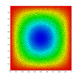
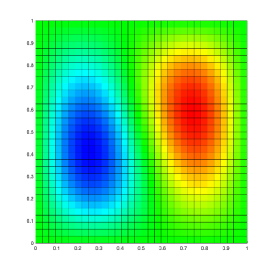
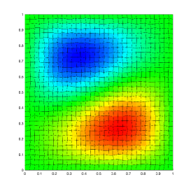
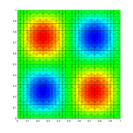
Figure 1: Test 1. Plots of the first four eigenfunctions for$\mathcal{T}_{h}^{1}$(top left) ,$\mathcal{T}_{h}^{2}$(top right), $\mathcal{T}_{h}^{3}$(bottom left) and $\mathcal{T}_{h}^{4}$(bottom right) with $N=32$

5.1 Effect of the stability constant

The aim of this test is to analyze the influence of the stability (see (5.1)) on the computed spectrum, to know whether the quality of the computations can be affected by this constant. We will consider the same geometrical configuration of the previous test. We will compute the lowest eigenvalue for different values $w_{\mathrm{K}}$ using the family of meshes $\mathcal{T}_{h}^{2}$ .

Table 2: Test 1. The lowest eigenvalue $\lambda_{h1}$ for $w_{\mathrm{K}}=0$ and $w_{\mathrm{K}}=4^{-k}$ with $-6\leq k\leq 6$ and $\mathcal{T}_{h}^{2}$.

$N$	$w_{\mathrm{K}}=4^{6}$	$w_{\mathrm{K}}=4^{5}$	$w_{\mathrm{K}}=4^{4}$	$w_{\mathrm{K}}=4^{3}$	$w_{\mathrm{K}}=4^{2}$	$w_{\mathrm{K}}=4^{1}$	$w_{\mathrm{K}}=4^{0}$
8	0.0623	0.2470	0.9530	3.3404	8.9395	15.3873	18.7724
16	0.2469	0.9521	3.3296	8.8625	15.1606	18.4360	19.4886
32	0.9519	3.3269	8.8434	15.1048	18.3535	19.3965	19.6760
64	3.3262	8.8386	15.0909	18.3330	19.3735	19.6524	19.7234
128	8.8374	15.0874	18.3279	19.3678	19.6465	19.7174	19.7352
256	15.0865	18.3266	19.3664	19.6450	19.7160	19.7338	19.7382
​​Order​​	0.3746	0.7304	1.1463	1.5302	1.8027	1.9400	1.9885
$\lambda_{1}$	19.7392	19.7392	19.7392	19.7392	19.7392	19.7392	19.7392
$N$	$w_{\mathrm{K}}=4^{-1}$	$w_{\mathrm{K}}=4^{-2}$	$w_{\mathrm{K}}=4^{-3}$	$w_{\mathrm{K}}=4^{-4}$	$w_{\mathrm{K}}=4^{-5}$	$w_{\mathrm{K}}=4^{-6}$	$w_{\mathrm{K}}=0$
8	19.8649	20.1582	20.2328	20.2516	20.2563	20.2575	20.2579
16	19.7708	19.8427	19.8607	19.8652	19.8664	19.8666	19.8667
32	19.7471	19.7650	19.7695	19.7706	19.7709	19.7709	19.7710
64	19.7412	19.7457	19.7468	19.7470	19.7471	19.7471	19.7471
128	19.7397	19.7408	19.7411	19.7412	19.7412	19.7412	19.7412
256	19.7393	19.7396	19.7397	19.7397	19.7397	19.7397	19.7397
​​Order​​	1.9978	2.0039	2.0049	2.0052	2.0052	2.0052	2.0052
$\lambda_{1}$	19.7392	19.7392	19.7392	19.7392	19.7392	19.7392	19.7392

It can be seen from Table 2 despite to the fact that the different stabilization numbers do not introduce spurious eigenvalues in the method, the order of convergence is affected when the stabilization constant is large.

5.2 Test 2: L-shaped domain

In this stage, we consider the classic non-convex domain called L-shaped domain. The non-convexity fo this geometry leads to obtain non-smooth eigenfunctions due the singularity and hence, non optimal order of convergence. Contrary to the square domain, for this test we do not have analytical solutions. Hence, we obtain the eigenvalues for different meshes and different refinement levels and compute the order of convergence respect to an extrapolated value, which is reported in the row ’Extrap.’ of Table 3. These extrapolated values have been computed by means of a least-square fitting.

In this test we have used four different families of meshes (see Fig. 2):

• $\mathcal{T}_{h}^{5}$: non-structured hexagonal meshes made of convex hexagons;

• $\mathcal{T}_{h}^{6}$: triangular meshes;

• $\mathcal{T}_{h}^{7}$: square meshes;

In Table 3 we report the first six eigenvalues of (2.1) computed with our mixed method in the L-shaped domain.

Table 3: Test 2. The lowest computed eigenvalues $\lambda_{hi}$, $1\leq i\leq 6$ for different $\mathcal{T}_{h}$.

$\mathcal{T}_{h}$	$N$	$\lambda_{h1}$	$\lambda_{h2}$	$\lambda_{h3}$	$\lambda_{h4}$	$\lambda_{h5}$	$\lambda_{h6}$
	18	37.7081	59.7051	76.6486	113.201	119.976	155.366
	38	38.3107	60.5558	78.4827	117.017	125.714	163.376
$\mathcal{T}_{h}^{5}$	54	38.4262	60.6812	78.7317	117.587	126.701	164.712
	70	38.4735	60.7270	78.8254	117.797	127.079	165.205
	90	38.4999	60.7511	78.8784	117.909	127.284	165.454
	Order	1.65	2.04	2.13	2.02	1.82	1.89
	Extrap.	38.5625	60.7943	78.9530	118.109	127.721	166.000
$\mathcal{T}_{h}$	$N$	$\lambda_{h1}$	$\lambda_{h2}$	$\lambda_{h3}$	$\lambda_{h4}$	$\lambda_{h5}$	$\lambda_{h6}$
	10	35.6472	56.2124	71.8313	102.1495	105.329	133.136
	20	37.6435	59.5705	77.0532	113.680	121.000	155.988
$\mathcal{T}_{h}^{6}$	30	38.0916	60.2398	78.0999	116.088	124.487	161.234
	50	38.3550	60.5895	78.646	117.359	126.413	164.123
	60	38.4064	60.6502	78.7409	117.580	126.763	164.641
	Order	1.68	1.90	1.89	1.84	1.73	1.70
	Extrap.	38.5495	60.8048	78.9882	118.184	127.800	166.259
$\mathcal{T}_{h}$	$N$	$\lambda_{h1}$	$\lambda_{h2}$	$\lambda_{h3}$	$\lambda_{h4}$	$\lambda_{h5}$	$\lambda_{h6}$
	20	37.1216	58.8887	76.4390	111.187	117.648	148.894
	40	38.0961	60.2981	78.3125	116.279	124.824	161.043
$\mathcal{T}_{h}^{7}$	60	38.3168	60.5690	78.6692	117.276	126.3007	163.633
	80	38.4047	60.6648	78.7948	117.629	126.846	164.582
	100	38.4497	60.7094	78.8530	117.793	127.110	165.034
	Order	1.66	1.94	1.96	1.92	1.83	1.79
	Extrap.	38.5476	60.7943	78.9613	118.111	127.635	166.007

From Table 3 we observe that the order of convergence for the first eigenvalue is not optimal. This is expectable due the non-convexity of the chosen domain. In the other hand, the rest of the eigenvalues converge to the extrapolated ones with double order, since in these cases, the singularity does not deteriorate the smoothness of the associated eigenfunctions.

In Figure 2 we present plots for the first two eigenfunctions of the Laplace eigenproblem in the L-shaped domain, computed with different type of meshes.

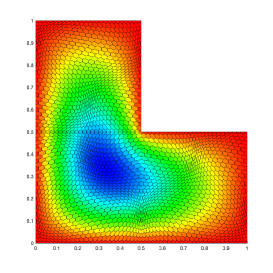
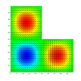
Figure 2: Test 2. Plots of the first two eigenfunctions for $\mathcal{T}_{h}^{5}$ (left) and $\mathcal{T}_{h}^{6}$ (right).

5.3 Square with mixed boundary conditions.

Let us mention the natural extension of system (2.1) to the mixed boundary conditions case. Let $\Omega\subset\mathbb{R}^{2}$ be an open bounded domain with Lipschitz boundary $\Gamma$. We assume that this boundary is splitted in two parts $\Gamma_{D}$ and $\Gamma_{N}$ such that $\Gamma:=\Gamma_{D}\cup\Gamma_{N}$. The Laplace eigenvalue problem reads as follows:

Problem 5.

Find $(\lambda,u)\in{\mathbb{R}}\times{\mathrm{H}^{1}(\Omega)}$, $u\neq 0$, such that

$$\left\{\begin{array}[]{l}-\Delta u=\lambda u\quad\text{in }\Omega,\\[2.84544pt] u=0\,\,\,\quad\quad\text{ on }\Gamma_{D}.\\ u\cdot\boldsymbol{n}=0\quad\text{ on }\Gamma_{N},\end{array}\right.$$ (5.3)

where $\boldsymbol{n}$ denotes the outward unitary vector respect to $\Gamma_{N}$. A mixed variational formulation of (5.3) is the following: Find $(\lambda,\boldsymbol{\sigma},u)\in{\mathbb{R}}\times\mathrm{H}_{0}(\mathop{\mathrm{div}}\nolimits,\Omega)\times\mathrm{L}^{2}(\Omega)$, $(\boldsymbol{\sigma},u)\neq(\boldsymbol{0},0)$, such that

$$\begin{split}\int_{\Omega}\boldsymbol{\sigma}\cdot\boldsymbol{\tau}+\int_{\Omega}\mathop{\mathrm{div}}\nolimits\boldsymbol{\tau}u=&0\qquad\forall\boldsymbol{\tau}\in\mathrm{H}_{0}(\mathop{\mathrm{div}}\nolimits,\Omega),\\ \int_{\Omega}\mathop{\mathrm{div}}\nolimits\boldsymbol{\sigma}v=&-\lambda\int_{\Omega}uv\qquad\forall v\in\mathrm{L}^{2}(\Omega).\end{split}$$

where the condition $u\cdot\boldsymbol{n}$ is imposed in the space $\mathrm{H}(\mathop{\mathrm{div}}\nolimits,\Omega)$. The analysis of this variational formulations is analogous to the Dirichlet boundary condition case considered before. The main difference lies on the regularity of the solution $u$, which is affected due the mixed boundary conditions (see [21]).

If the $\Omega$-domain is convex, the analysis of convergence and error estimates holds with no major changes. However, for non-convex domains the analysis is more complex and this will be studied in a future work.

In the present test we consider as computational domain the square $\Omega:=(-1,1)^{2}$. The boundary conditions provided in (2.1) are imposed as follows: the condition $u=0$ (i.e., condition on $\Gamma_{D}$) is considered in the top and bottom of the square, meanwhile the condition on $\Gamma_{N}$ is considered on the other two sides of the square.

We begin with the analysis of the effects of the stabilization $w_{\mathrm{K}}$ in the computation of the spectrum. Since we have mixed boundary conditions, which is obviously different compared with our already presented experiments only for the boundary condition $u=0$, it is expectable that spurious modes can arise for certain stabilizations. The following tables report computed eigenvalues for two different meshes: one of triangles ($\mathcal{T}_{h}^{1}$) and the other of squares ($\mathcal{T}_{h}^{2}$). We present this two choices only for simplicity. We mention that for other polygonal meshes the results are similar.

For the experiments, we fix $\mathcal{T}_{h}^{1}$ and $\mathcal{T}_{h}^{2}$ in $N=10$. In tables 4 and 5 we report the first ten eigenvalues computed with our method, considering the meshes mentioned before and for different values of $w_{\mathrm{K}}$. The numbers in boxes represent spurious eigenvalues and the last column present the exact eigenvalues of the problem, which we compare with the computed ones.

Table 4: Test 3. Computed lowest eigenvalues for different values of $w_{\mathrm{K}}$ with $N=10$.

$\mathcal{T}_{h}^{1}$
$w_{\mathrm{K}}=0$	$w_{\mathrm{K}}=\frac{1}{100}$	$w_{\mathrm{K}}=\frac{1}{10}$	$w_{\mathrm{K}}=\frac{1}{4}$	$w_{\mathrm{K}}=\frac{1}{2}$	$\lambda_{hi}$
2.4718	2.4716	2.4691	2.4650	2.4582	2.4674
4.9502	4.9490	4.9385	4.9212	4.8925	4.9348
9.9277	9.9230	9.8810	9.8118	9.6984	9.8701
12.4172	12.4101	12.3466	12.2403	12.0572	12.3373
12.4407	12.4329	12.3634	12.2511	12.0779	12.3374
20.0183	19.9999	19.8354	19.5668	19.1338	19.7404
22.5181	22.4946	22.2854	21.9447	21.3974	22.2094
25.0231	24.9958	24.7517	24.3525	23.6593	24.6753
25.1170	25.0863	24.8131	24.3723	23.7235	24.6757
32.6591	32.6124	32.1980	31.5263	30.4107	32.0801
$w_{\mathrm{K}}=1$	$w_{\mathrm{K}}=1.5$	$w_{\mathrm{K}}=2$	$w_{\mathrm{K}}=5$	$w_{\mathrm{K}}=10$	$\lambda_{hi}$
2.4447	2.4314	2.4182	2.3416	2.2236	2.4674
4.8362	4.7810	4.7270	4.4256	3.9962	4.9348
9.4787	9.2680	9.0657	8.0046	6.6680	9.8701
11.6989	11.3597	11.0385	9.4235	7.5451	12.3373
11.7524	11.4439	11.1505	9.6523	7.8569	12.3374
18.3195	17.5672	16.8702	13.5654	10.0645	19.7404
20.3747	19.4378	18.5765	14.5876	10.5526	22.2094
22.3529	21.1738	20.1051	15.3520	10.9359	24.6753
22.5443	21.4719	20.4918	16.0154	11.5723	24.6757
28.2992	26.4446	24.8059	17.9568	12.0748	32.0801

Table 5: Test 3. Computed lowest eigenvalues for different values of $w_{\mathrm{K}}$ with $N=10$.

$\mathcal{T}_{h}^{2}$
$w_{\mathrm{K}}=0$	$w_{\mathrm{K}}=\frac{1}{100}$	$w_{\mathrm{K}}=\frac{1}{10}$	$w_{\mathrm{K}}=\frac{1}{4}$	$w_{\mathrm{K}}=\frac{1}{2}$	$\lambda_{hi}$
2.5086	2.5073	2.4960	2.4775	2.4472	2.4674
5.0171	5.0146	4.9921	4.9550	4.8943	4.9348
10.5573	10.5350	10.3390	10.0279	9.5492	9.8701
13.0658	13.0423	12.8350	12.5054	11.9963	12.3373
13.0658	13.0423	12.8350	12.5054	11.9963	12.3374
21.1146	21.0701	20.6780	20.0559	19.0983	19.7404
25.9616	25.8275	24.6801	22.9788	20.6107	22.2094
28.4702	28.3348	27.1762	25.4563	23.0579	24.6753
28.4702	28.3348	27.1762	25.4563	23.0579	24.6757
36.5189	36.3626	35.0191	33.0067	30.1599	32.0801
$w_{\mathrm{K}}=1$	$w_{\mathrm{K}}=1.5$	$w_{\mathrm{K}}=2$	$w_{\mathrm{K}}=5$	$w_{\mathrm{K}}=10$	$\lambda_{hi}$
2.3887	2.3330	2.2798	2.0055	1.6705	2.4674
4.7774	4.6660	4.5596	4.0110	3.3409	4.9348
8.7168	8.0179	7.4227	5.1355	3.3930	9.8701
11.1055	10.3509	9.7025	7.1410	4.1925	12.3373
11.1055	10.3509	9.7025	7.1410	4.5674	12.3374
17.0886	14.5946	12.7359	7.2193	4.7619	19.7404
17.4335	16.0357	14.8455	8.4073	4.8714	22.2094
19.4774	16.9276	15.0157	9.0909	4.9359	24.6753
19.4774	16.9276	15.0157	9.2247	4.9737	24.6757
25.6777	20.4314	16.9652	9.2247	4.9937	32.0801

We observe from tables 4 and 5 that the behaviour of the spurious eigenvalues clearly depend on the choice of $w_{\mathrm{K}}$. Notice that when $w_{\mathrm{K}}$ is close to zero (even for the case $w_{\mathrm{K}}=0$) the spurious vanish, meanwhile when $w_{\mathrm{K}}$ increases, the spurious eigenvalues appear, for both $\mathcal{T}_{h}^{1}$ and $\mathcal{T}_{h}^{2}$, from $w_{\mathrm{K}}=5$ in forward. Moreover, we observe that the method do not introduce spurious for $w_{\mathrm{K}}<2$. This phenomenon is analogous for other meshes.

We remark that the appearance of spurious eigenvalues is not visible for the domain with the Dirichlet boundary condition, which leads to conclude that the mixed boundary is also a relevant factor at the moment to compute the spectrum of the Laplace eigenvalue problem.

Now we are interested to observe if the refinement of the meshes influence the appearance of spurious eigenvalues when we choose a value of $w_{\mathrm{K}}$ that introduces pollution of the spectrum. To do this task, we chose $w_{\mathrm{K}}=10$ (since with this value of $w_{E}$ several spurious eigenvalues are observed) and refine the meshes $\mathcal{T}_{h}^{1}$ and $\mathcal{T}_{h}^{2}$ that we have used in the previous tests.

Table 6: Test 3. Computed lowest eigenvalues for $w_{\mathrm{K}}=10$.

$\mathcal{T}_{h}^{1}$
$\lambda_{hi}$	$N=10$	$N=20$	$N=30$	$N=40$
2.4674	2.2236	2.4071	2.4399	2.4520
4.9348	3.9962	4.6921	4.8230	4.8729
9.8701	6.6680	8.9636	9.4461	9.6299
12.3373	7.5451	10.9239	11.6687	11.9544
12.3373	7.8569	10.9440	11.6810	11.9617
19.7404	10.0645	16.4216	18.0867	18.8010
22.2094	10.5526	18.0007	20.1514	21.0296
24.6753	10.9359	19.5387	22.0980	23.1650
24.6757	11.5723	19.8019	22.1888	23.2291
32.0801	12.0748	23.9208	27.8445	29.5927
$\mathcal{T}_{h}^{2}$
$\lambda_{hi}$	$N=10$	$N=20$	$N=30$	$N=40$
2.4674	1.6705	2.2045	2.3432	2.3960
4.9348	3.3409	4.4090	4.6864	4.7919
9.8701	3.3930	6.6819	8.1431	8.8180
12.3373	4.1925	8.8864	10.4863	11.2139
12.3373	4.5674	8.8864	10.4863	11.2139
19.7404	4.7619	10.7096	15.0342	17.5084
22.2094	4.8714	12.9141	16.2862	17.6359
24.6753	4.9359	12.9141	17.3774	19.9043
24.6757	4.9737	13.3637	17.3774	19.9043
32.0801	4.9937	13.5721	21.3607	26.3263

From table 6 we observe that the spurious eigenvalues disappear when the meshes are refined, which is expectable, since the accuracy of the VEM is improved when the meshes are refined. Similar results have been obtained for other numerical methods that depend on some particular stabilization parameter (for instance, the DG method [24, 23]).

In table 7 we report the first six eigenvalues computed with our method considering different polygonal meshes and $w_{\mathrm{K}}=1$. It is clear that the double order of convergence is obtained with this configuration of the geometry, as is expected.

Table 7: Test 3. The lowest computed eigenvalues $\lambda_{hi}$, $1\leq i\leq 6$ for different $\mathcal{T}_{h}$.

$\mathcal{T}_{h}$	$N$	$\lambda_{h1}$	$\lambda_{h2}$	$\lambda_{h3}$	$\lambda_{h4}$	$\lambda_{h5}$	$\lambda_{h6}$
	8	2.4343	4.8005	9.3442	11.4928	11.5519	17.7203
	16	2.4592	4.9004	9.7437	12.1144	12.1295	19.2004
$\mathcal{T}_{h}^{1}$	32	2.4653	4.9263	9.8362	12.2820	12.2839	19.6013
	64	2.4669	4.9327	9.8613	12.3237	12.3239	19.7054
	Order	2.0200	1.9600	2.0800	1.9100	1.9100	1.8900
	Extr.	2.4673	4.9351	9.8670	12.3406	12.3391	19.7470
	8	2.3465	4.6931	8.1753	10.5219	10.5219	16.3507
	16	2.4361	4.8722	9.3862	11.8223	11.8223	18.7724
$\mathcal{T}_{h}^{2}$	32	2.4595	4.9190	9.7443	12.2038	12.2038	19.4886
	64	2.4654	4.9308	9.8380	12.3034	12.3034	19.6760
	Order	1.9400	1.9400	1.7900	1.8000	1.8000	1.7900
	Extr.	2.4676	4.9353	9.8822	12.3496	12.3496	19.7644
	8	2.3474	4.6887	8.1662	10.4683	10.5147	16.3106
	16	2.4363	4.8705	9.3909	11.8172	11.8204	18.7349
$\mathcal{T}_{h}^{3}$	32	2.4596	4.9186	9.7456	12.2024	12.2029	19.4837
	64	2.4654	4.9308	9.8383	12.3032	12.3032	19.6746
	Order	1.9500	1.9300	1.8100	1.8300	1.8000	1.7400
	Extr.	2.4675	4.9354	9.8811	12.3473	12.3495	19.7787
	8	2.3575	4.6664	8.3096	10.4737	10.5728	16.0176
	16	2.4390	4.8649	9.4302	11.8119	11.8429	18.6639
$\mathcal{T}_{h}^{4}$	32	2.4603	4.9171	9.7561	12.2014	12.2096	19.4593
	64	2.4656	4.9304	9.8410	12.3028	12.3049	19.6685
	Order	1.9500	1.9300	1.8100	1.8100	1.8200	1.7700
	Extr.	2.4676	4.9355	9.8799	12.3491	12.3477	19.7701

Finally, in figure 3 we present plots of the first four eigenfunctions for the Laplace eigenvalue problem with mixed boundary conditions, obtained with different polygonal meshes.

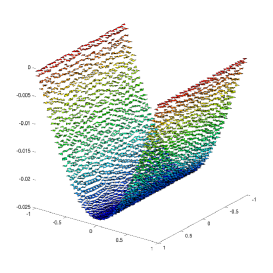
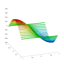
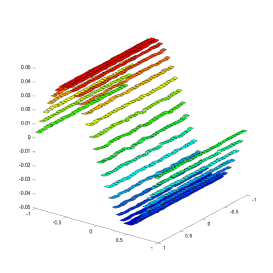
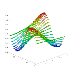
Figure 3: Test 3. Plots of the first four eigenfunctions for $\mathcal{T}_{h}^{1}$ (top left), $\mathcal{T}_{h}^{2}$ (top right), $\mathcal{T}_{h}^{3}$ (bottom left) and $\mathcal{T}_{h}^{4}$ (bottom right) computed with different meshes and $N=32$.

References

• [1] S. Agmon, Lectures on Elliptic Boundary Value Problems, Van Nostrand Mathematical Studies, No. 2. D (B. F. Jones Jr & G. W. Batten Jr, eds.). Princeton, NJ; Toronto-London: Van Nostrand, (1965).
• [2] P. F. Antonietti, L. Beirão da Veiga, D. Mora, and M. Verani, A stream virtual element formulation of the Stokes problem on polygonal meshes, SIAM J. Numer. Anal., 52 (2014), pp. 386–404.
• [3] I. Babuška and J. Osborn, Eigenvalue problems, in Handbook of Numerical Analysis, Vol. II, P.G. Ciarlet and J.L. Lions, eds., North-Holland, Amsterdam, 1991, pp. 641–787.
• [4] L. Beirão da Veiga, F. Brezzi, A. Cangiani, G. Manzini, L. D. Marini and A. Russo, Basic principles of virtual element methods, Math. Models Methods Appl. Sci., 23 (2013), pp. 199–214.
• [5] L. Beirão da Veiga, F. Brezzi, L. D. Marini and A. Russo, Mixed virtual element methods for general second order elliptic problems on polygonal meshes. ESAIM Math. Model. Numer. Anal., 50 (2016), pp. 727–747.
• [6] L. Beirão da Veiga, F. Brezzi, L. D. Marini and A. Russo, The Hitchhiker’s guide to the virtual element method, Math. Models Methods Appl. Sci., 24 (2014), pp. 1541–1573.
• [7] L. Beirão da Veiga, C. Lovadina and G. Vacca, Divergence free virtual elements for the Stokes problem on polygonal meshes, ESAIM Math. Model. Numer. Anal., 51, (2017), pp. 509–535.
• [8] L. Beirão da Veiga, D. Mora, G. Rivera and R. Rodríguez, A virtual element method for the acoustic vibration problem, Numer. Math., 136 (2017), pp. 725–763.
• [9] F. Brezzi, R. S. Falk and L. D. Marini, Basic principles of mixed virtual element methods. ESAIM Math. Model. Numer. Anal. 48, 1227–1240 (2014).
• [10] D. Boffi, Finite element approximation of eigenvalue problems, Acta Numerica, 19 (2010), pp. 1–120.
• [11] D. Boffi, F. Brezzi and M. Fortin, Mixed Finite Element Methods and applications. Springer Series in Computational Mathematics, 44. Springer, Heidelberg (2013).
• [12] E. Cáceres and G. N. Gatica, A mixed virtual element method for the pseudostress-velocity formulation of the Stokes problem, IMA J. Numer. Anal., 37, pp. 296–331 (2017).
• [13] E. Cáceres, G. N. Gatica and F. A. Sequeira, A mixed virtual element method for the Brinkman problem, Math. Models Methods Appl. Sci., 27 (2017), pp. 707–743.
• [14] O. Čertík, F. Gardini, G. Manzini, L. Mascotto and G. Vacca, The p- and hp-versions of the virtual element method for elliptic eigenvalue problems, Comput. Math. Appl., 79, (2020), pp. 2035–2056.
• [15] J. Descloux, N. Nassif, and J. Rappaz, On spectral approximation. part 1. the problem of convergence, ESAIM: Mathematical Modelling and Numerical Analysis-Modélisation Mathématique et Analyse Numérique, 12 (1978), pp. 97–112.
• [16] J. Descloux, N. Nassif, and J. Rappaz, On spectral approximation. part 2. error estimates for the Galerkin method, RAIRO. Analyse numérique, 12 (1978), pp. 113–119.
• [17] F. Gardini, G. Manzini, and G. Vacca, The nonconforming virtual element method for eigenvalue problems, ESAIM Math. Model. Numer. Anal., 53, (2019), pp. 749–774.
• [18] F. Gardini and G. Vacca, Virtual element method for second-order elliptic eigenvalue problems, IMA J. Numer. Anal. 38, (2018), pp. 2026-2054.
• [19] G.N. Gatica, M. Munar and F. A. Sequeira, A mixed virtual element method for a nonlinear Brinkman model of porous media flow, Calcolo, 55, (2018), article:21.
• [20] G. N. Gatica, M. Munar and F. A. Sequeira A mixed virtual element method for the Navier-Stokes equations, Mathematical Models and Methods in Applied Sciences, 28, (2018), pp. 2719–2762.
• [21] P. Grisvard, Problèmes aux limites dans les polygones. Mode d’emploi, EDF Bull. Direction Études Rech. Sér. C Math. Inform., (1986), pp. 3, 21–59.
• [22] T. Kato, Perturbation Theory for Linear Operators, Springer Verlag, Berlin, 1995.
• [23] F. Lepe, S. Meddahi, D. Mora and R. Rodríguez, Mixed discontinuous Galerkin approximation of the elasticity eigenproblem, Numer. Math., 142 (2019), pp. 749–786.
• [24] F. Lepe and D. Mora, Symmetric and nonsymmetric discontinuous Galerkin methods for a pseudo stress formulation of the Stokes spectral problem, SIAM J. Sci. Comput., 42, 2, pp. A698–A722, (2020).
• [25] F. Lepe, D. Mora, G. Rivera and I. Velásquez, A virtual element method for the Steklov eigenvalue problem allowing small edges, Preprint, arXiv:2006.09573 [math.NA] (2020).
• [26] J. Meng and L. Mei, A linear virtual element method for the Kirchhoff plate buckling problem, Appl. Math. Lett., 103, (2020), 106188, 8 pp.
• [27] J. Meng, Y. Zhang, and L. Mei, A virtual element method for the Laplacian eigenvalue problem in mixed form, Appl. Numer. Math., 156 (2020), pp. 1–13.
• [28] D. Mora and G. Rivera, A priori and a posteriori error estimates for a virtual element spectral analysis for the elasticity equations, IMA J. Numer. Anal., 40 (2020), pp. 322–357.
• [29] D. Mora, G. Rivera and R. Rodríguez, A virtual element method for the Steklov eigenvalue problem, Math. Models Methods Appl. Sci., 25, (2015), pp. 1421–1445.
• [30] D. Mora and I. Velásquez, Virtual element for the buckling problem of Kirchhoff-Love plates, Comput. Methods Appl. Mech. Engrg., 360, (2020), 112687, 22 pp.