Charge regulation of colloidal particles in aqueous solutions

Abstract

We study charge regulation of colloidal particles inside aqueous electrolyte solutions. To stabilize colloidal suspension against precipitation, colloidal particles are synthesized with either acidic or basic groups on their surface. In contact with water these surface groups undergo proton transfer reaction, resulting in colloidal surface charge. The charge is determined by the condition of local chemical equilibrium between hydronium ions inside the solution and at the colloidal surface. We use a model of Baxter sticky spheres to explicitly calculate the equilibrium dissociation constants and to construct a theory which is able to quantitatively predict the effective charge of colloidal particles with either acidic or basic surface groups. The predictions of the theory for the model are found to be in excellent agreement with the results of Monte Carlo simulations. The theory is further extended to treat colloidal particles with a mixture of both acidic and basic surface groups.

I Introduction

Aqueous solutions are of great importance in biology and chemistry ro1997 ; ANDELMAN1995 ; Messina_2009 ; Abrashkin . In many cases such solutions are ionic. The long-range Coulomb interaction between charged particles is the mains source of difficulty for exploring the thermodynamics of such systems levin ; shen2017electrostatic ; smith2016electrostatic ; adar2018dielectric ; Krishnan3 ; Frydeloettel ; walker2011 . Because of organic functional groups many surfaces and membranes acquire surface charge when placed in water. From their interaction with water and acid or base these functional groups can either lose or gain a proton, becoming charged alexander1984 ; trizac2002 . The amount of charge gained in this process depends on the pH of solution adamson ; Dawei and the process is known as charge regulation (CR) bakhshandeh2019 ; podgornik2018 ; frydel2019 ; avni2019charge ; lind ; majee2019 ; Yael2018 ; chan71white ; pericet2004 ; VONGRUNBERG1999339 ; ozcelik2019electric ; Podgornikexpansion ; van2018solution ; Markovich_2016 ; avni2019charge ; Krishnan1 ; Krishnan2 ; Hartvig . CR is of great importance in colloidal science, biology, and chemistry prieve1976 ; carnie1993 ; netz2002 ; Majee ; hallett ; lowen1 ; monica1 ; monica2 ; ZANDI2020 ; roshal2019ph ; javidpour2019role ; Zahler ; PodgornikpH ; Mikaellund ; SHEN200592 ; Biesheuvel ; Narahari ; Burak ; Kumar ; Fleck ; Lund2013 ; Grant2001 ; Elcock2001 ; Lund2005 ; Mason2008 ; Aguilar2010 ; Stahlberg1996 ; Tsao2000 ; Philippe , and is responsible for the stability of many different systems Markovich_2017 ; podgornik1991 ; leckband ; Borkovecl2016 ; Maarten ; Jyh-Ping ; WOLTERINK200613 ; Ionel ; Gong ; Holger1999 .

The concept of charge regulation was first described by Linderstrøm-Lang and later developed by many other researchers lind ; kirkwood1952 ; marcus1955 ; lifson1957 ; PodgornikA2014 ; SMITH2020 ; safinya_h . The first quantitative implementation of charge regulation was done by Ninham and Parsegian (NP) ninham1971 who combined the idea of the local chemical equilibrium with the Poisson-Boltzmann theory introduced by Gouy and Chapman sixty years earlier chapman19 ; gouy1910 . The fundamental assumption of the NP theory is that the bulk association constants can be used to study proton transfer reactions with the surface adsorption sites. Within the NP approach the bulk concentration of hydronium ions is replaced by the local density determined self consistently by the Boltzmann distribution,

$$c_{\ch{H+}}^{surf}=c_{\ch{H_{3}O+}}^{bulk}\exp({-\beta\phi_{0}}),$$ (1)

where $\beta=1/k_{B}T$ and $\phi_{0}$ the electrostatic surface potential.

The NP theory relies on Poisson-Boltzmann equation with the CR implemented as a new boundary condition. The two parameters that determine the boundary condition are the equilibrium constant of the chemical reaction taking place at the surface, and the surface density of the chemical groups. Within the NP model, the surface is homogeneous, therefore, the model ignores the discrete structure of surface chemical groups. Another assumption is that the equilibrium constant is defined in terms of the concentrations of the reacting species rather than their activities. The validity of this assumption needs to be tested, since the concentration of hydronium ions can be quite large near a charged surface. Finally, the value of the equilibrium constant at the surface is assumed to be the same as for the reaction in the bulk. This is clearly far from obvious.

In this paper we will focus on spherical colloidal particles with acidic and basic surface groups. If a colloidal particle has $N_{site}$ basic functional groups on its surface then the effective surface charge within the NP theory is found to be

$$\sigma=\frac{K_{Bulk}N_{site}q~{}c_{a}~{}\mathrm{e}^{-\beta\phi_{0}}}{4~{}\pi~{}(a+r_{ion})^{2}(1+K_{Bulk}~{}c_{a}~{}\mathrm{e}^{-\beta\phi_{0}})},$$ (2)

where $a$ is the colloidal radius and $c_{a}$ is the bulk concentration of strong acid. On the other hand if the surface has $N_{site}$ acidic groups, the effective surface charge is

$$\sigma=-\frac{N_{site}~{}q}{4\pi(a+r_{ion})^{2}}+\frac{K_{Bulk}N_{site}q~{}c_{a}~{}\mathrm{e}^{-\beta\phi_{0}}}{4~{}\pi~{}(a+r_{ion})^{2}(1+K_{Bulk}~{}c_{a}~{}\mathrm{e}^{-\beta\phi_{0}})},$$ (3)

where $K_{Bulk}$ is the bulk equilibrium association constant, which is the inverse of the acid dissociation constant $K_{a}$, and $q$ is the elementary proton charge. The electrostatic surface potential $\phi_{0}$ must be calculated self-consistently by combining these expressions with the mean-field Poisson-Boltzmann equation.

The fundamental ingredient of the NP theory is the equilibrium constant. In the original approach the equilibrium constant for the active sites on the colloidal surface was assumed to be the same as for the bulk solution, however, in the latter works the equilibrium constant was treated as a fitting parameter. Clearly this is not very satisfactory, since it does not allow us to explicitly probe the validity of the theory. Although, the NP theory was a pioneering first step in understanding charge regulation in colloidal systems, in the absence of an explicit model on which the theory could be tested, the validity of the underlying approximations of the theory remains unclear. A different approach was recently advocated by Bakhshandeh et al. in which a specific model of of association was used to calculate exactly the bulk equilibrium constant for acid bakhshandeh2019 . The same acidic groups where then placed on top of a spherical colloidal particle and the density profiles for hydronium cations and corresponding anions were calculated exactly – within this model – using Monte Carlo simulations. Knowledge of the exact equilibrium constant allowed us to explicitly compare the results of simulations with the NP theory. It was found that NP approach deviated significantly from the predictions of simulations. For the specific case of acidic surface groups Ref. bakhshandeh2019 then introduced an alternative approach which was found to be in excellent agreement with the Monte Carlo simulations. The objective of this paper is to extend the results of bakhshandeh2019 to colloidal particles with basic surface groups, as well to the particles containing a mixtures of basic and acidic surface groups.

We should note that the present theory applies directly only to the specific model of chemical association described below. There are two levels of approximation that we use: 1 – the microscopic model of acid-base association in terms of the Baxter sticky spheres, and 2 – the approximations used to theoretically solve the model. The advantage of this two step approach is that the theory can be tested against an “exact” solution of the microscopic model obtained using the computer simulations. This allows us to separate the possible shortfalls of the theory from those of the microscopic model. If the theory agrees with the “exact” solution of the model, any shortfalls can then be attributed to the microscopic model of association and not to the approximations which had to be made to solve the model. The disadvantage of such approach is that the theory that we develop applies only to the specific microscopic model of acid/base equilibrium and is not generally universal. This, however, is the problem with any microscopic theory which does not explicitly take into account all the quantum effects associated with the charge transfer at the interface. In the absence of such “complete” theory, we expect that the approach advocated in the present paper will help to shed interesting new light on the mechanisms of charge regulation of nanoparticles and colloidal suspensions, and in particular on applicability of mean-field theories to study this intrinsically strong-coupling problem.

There are several possibilities for colloidal surface to acquire charge. The acidic functional groups, such as carboxyl COOH, can become dissociated due to the following reaction

$$\ch{HA}+\ch{H_{2}O}\rightleftarrows\ch{H_{3}O+}+\ch{A-},$$ (4)

resulting in a negatively charged surface. Alternatively, basic functional groups, which originally are not charged, can gain protons from hydronium ions and acquire a positive charge,

$$\ch{B}+\ch{H_{3}O+}\rightleftarrows\ch{H_{2}O}+\ch{HB+}.$$ (5)

One example of such functional group is amine NH2.

The paper is organized as follows. In section II, we introduce a model of a colloidal particles with sticky sites and present the details of Monte Carlo simulations. In section III we show how the equilibrium association constant can be calculated for sticky ions. In section IV we present a model for a uniformly sticky colloidal particle. In Section V this model is extended to account for discrete basic surface groups, and in Section VI and VII to discrete acidic groups. In Section VIII we consider particles with a mixture of both basic and acidic surface groups and in Section IX we present our conclusions.

II Theoretical background and Monte Carlo simulations details

II.1 Theoretical background

To study charge regulation of a colloidal surface we use a model of Baxter sticky spheres baxter ; frydel2019 ; frydel2019_2 . The sticky potential was previously used to study gelation in globular proteins Frenkel2003 ; Foffi2005 , chemical association in weak acid-base reactions Herrera , and sticky-charged wall model Blum ; Huckaby ; Jeffery ; Greathouse . In our model, sticky interactions take on a physical interpretation of a chemical bond between proton and acid/base groups. This is not the first time that a sticky interaction is used to model a chemical bond, to capture some aspect of quantum mechanics in an otherwise classical description. The idea has been around for some time and reaches back to 1980 in particular, the work of Blum and Herrera Blum ; Herrera , and Werthaim Wertheim1986 for directional chemical bonding. Sticky interactions continue to this day being an important part of soft-matter modeling Wang2012 . In the present work sticky interactions, and their quantum-chemical interpretation, will be used to study charge regulation of nanoparticles with surface acid and base groups. The results obtained, therefore, are only valid within the specific microscopic model. The model, of course, can be extended and modified to represent a different charge regulated system. For example, directional chemical bonding could be introduced by making a sphere sticky in limited regions. The size and shape of an absorbing molecule could be changed. These alternatives are not explored in the present work.

The hydronium ion can become adsorbed on an acidic or basic functional group to form a molecule H^+A^- or H^+B, respectively. To model the binding between H+ and A^- or B we use an attractive square well potential with a repulsive hard core frydel2019 ; bakhshandeh2019 . The first component of the interaction potential is the hard-core repulsion,

$$u_{hs}(r)=\begin{cases}\infty,&r<d,\\ 0,&r>d,\end{cases}$$ (6)

where $d$ is the diameter of particles. The second component is a narrow attractive well,

$$u_{well}(r)=\begin{cases}0,&r<d,\\ -\varepsilon,&d<r<d+\Delta,\\ 0,&r>d+\Delta.\end{cases}$$ (7)

To generalize the model, we also include a soft potential $u_{sf}(r>d)$, so that the total pair potential becomes $u_{tot}=u_{hs}+u_{well}+u_{sf}$,

$$u_{tot}(r)=\begin{cases}\infty,&r<d,\\ -\varepsilon+u_{sf}(r),&d<r<d+\Delta,\\ u_{sf}(r),&r>d+\Delta.\end{cases}$$ (8)

We note that the soft potential $u_{sf}(r)$ is effective from $r=d$, as illustrated in Fig. (1).

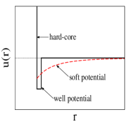
Figure 1: Schematic representation of the sticky-hard-sphere potential plus soft interaction. The sticky part is represented as a narrow well potential; (a) depicts hard-core plus attractive well and soft potential separately, and (b) as a combination. An important observation is that the soft interaction is active within the attractive well.

For illustration, we consider a very simple scenario comprised of two particles interacting via a pair potential in Eq. (8) and confined to a spherical region of radius $R$. To make the demonstration even simpler, one particle is fixed at the origin and only a second particle is free. The resulting partition function has two parts,

$$\cal{Z} =4\pi\int_{d}^{R}r^{2}e^{-\beta[u_{well}(r)+u_{sf}(r)]}dr=$$ (9)

$$4\pi e^{\beta\varepsilon}\int_{d}^{d+\Delta}r^{2}e^{-\beta u_{sf}(r)}dr+4\pi\int_{d+\Delta}^{R}r^{2}e^{-\beta u_{sf}(r)}dr.$$

Assuming a small $\Delta$, we can expand $\cal{Z}$ in $\Delta$, yielding

$$\cal{Z} = 4\pi d^{2}e^{\beta\varepsilon}e^{-\beta u_{sf}(d)}\bigg{[}\Delta\bigg{(}1-e^{-\beta\varepsilon}\bigg{)}$$ (10)

$$~{}+~{}\bigg{(}\frac{1}{d}-\frac{1}{2}\frac{d\beta u_{sf}(r)}{dr}\bigg{|}_{r=d}\bigg{)}\Delta^{2}+\dots\bigg{]}$$

$$~{}+~{}4\pi\int_{d}^{R}r^{2}e^{-\beta u_{sf}(r)}dr.$$

In the limit $\Delta\to 0$ only the last term does not vanish. However, if, at the same time as $\Delta\to 0$, $\varepsilon\to\infty$, then some of the expansion terms must also be retained. The correct way to carry out the limit is to require that $\Delta e^{\beta\varepsilon}=\rm{const}$, which is referred to as the Baxter limit baxter , and yields

$${\lim_{\begin{subarray}{c}\Delta\to 0\\ \varepsilon\to\infty\end{subarray}}}{\cal{Z}}=4\pi d^{2}l_{g}e^{-\beta u_{sf}(d)}+4\pi\int_{d}^{R}r^{2}e^{-\beta u_{sf}(r)}dr,$$ (11)

where we introduced the “sticky length” defined as

$$l_{g}=\lim_{\begin{subarray}{c}\varepsilon\to\infty\\ \Delta\to 0\end{subarray}}\Delta e^{\beta\varepsilon}.$$ (12)

Of great concern for simulations is the width $\Delta$ of the well potential, since in practice the exact Baxter limit cannot be attained and $\Delta$ must remain finite. To estimate what is sufficiently small value of $\Delta$, we consider the previous simple system with $u_{sf}=0$, for which the exact partition function is

$${\cal{Z}}=4\pi d^{2}l_{g}\bigg{[}1+\frac{\Delta}{d}+\frac{1}{3}\bigg{(}\frac{\Delta}{d}\bigg{)}^{2}\bigg{]}+\frac{4\pi R^{3}}{3}\bigg{[}1-\bigg{(}\frac{d+\Delta}{R}\bigg{)}^{3}\bigg{]}.$$ (13)

If we ignore the second term in square brackets, assuming $R\gg d$, we conclude that the well potential becomes sticky if $\Delta/d\ll 1$. In practice, we find that $\Delta/d\approx 0.01$ is sufficiently small to suppress most contributions of finite $\Delta$.

The Baxter sticky potential may appear analogous to a delta function potential often used in quantum mechanics. This, however, is misleading. The well potential in Eq. (7) transforms into the delta function in the limits $\Delta\to 0$ and $\varepsilon\to\infty$, while the product $\Delta\varepsilon$ is held fixed. On the other hand, the Baxter limit, requires that $\Delta e^{\beta\varepsilon}$ remains constant. To see this more clearly frydel2019 we define

$$f(r)=\begin{cases}\frac{1}{\Delta},&d\leq r\leq d+\Delta,\\ 0,&r<d~{}\text{or }~{}r>d+\Delta.\end{cases}$$ (14)

The Boltzmann factor then can be written as

$$e^{-\beta u_{well}(r)}=1+\Delta(\mathrm{e}^{\beta\epsilon}-1)f(r),$$ (15)

which in the Baxter limit reduces to

$$\lim_{\begin{subarray}{c}\varepsilon\to\infty\\ \Delta\to 0\end{subarray}}e^{-\beta u_{well}(r)}=1+l_{g}\delta(r-d),$$ (16)

with the sticky length given by $l_{g}\equiv\Delta(\mathrm{e}^{\beta\epsilon}-1)$. In the Baxter limit the $-1$ in the definition of $l_{g}$ can be neglected, however, in the simulations with finite $\Delta$ we will use the exact expression for $l_{g}$. The sticky potential itself is then

$$\beta u_{well}(r)=-\ln\bigg{[}1+l_{g}\delta(r-d)\bigg{]},$$ (17)

which shows that it is weaker than the delta function potential. Indeed, a delta function potential would result in an irreversible association between the sticky spheres. Finally, we note that if the expression (16) is used in the partition function Eq. (9), we will arrive directly at the Eq. (11).

II.2 Monte Carlo simulations details

We are now in a position to implement numerical simulations. The simulations are performed inside a spherical Wigner-Seitz (WS) cell of radius $R$. A spherical colloidal particle of radius $a$ is placed in the center of the WS cell. The radius of the cell is determined by the colloidal volume fraction of the suspension, $\varphi_{c}=a^{3}/R^{3}$. The motivation for using WS is that for small salt concentration colloidal system may crystallize, in which case thermodynamics will be very well described by the WS cell model, with a Donnan potential used to control the charge neutrality. In fact, even for the disordered state the WS approach to thermodynamics is found to lead to osmotic pressures in excellent agreement with experiments tamashirodonnan . In a sense, the many body colloid-colloid interactions in the grand-canonical ensemble are all included through the boundary condition of vanishing electric field at the WS cell boundary.

The colloidal particle has $N_{site}$ adsorption sites randomly distributed over its surface. Each adsorption site is a sphere of diameter $d$, see Fig. 2. If an active site is basic – has zero charge — it interacts with the hydronium ions through the hard core and the Baxter sticky potential, Eq.(8). On the other had if the site is acidic — has charge $-q$, where $q$ is the proton charge — in addition to the Baxter and hard core interactions, there is also a long range Coulomb potential between the adsorption site and all the ions inside simulation cell. In this work all the ions and the adsorption sites have diameter $4$ Å  and the colloidal particle has radius of $a=100$ Å.

The system is connected to a reservoir of strong acid at concentration $10^{-pH}$, and a reservoir of 1:1 strong electrolyte at concentration $c_{s}$.

Figure 2: The Baxter’s sticky spherical sites on the colloidal surface.

The solvent is considered to be a uniform dielectric of permittivity $\epsilon_{w}=80\epsilon_{0}$ and the Bjerrum length is $\lambda_{B}=q^{2}/\epsilon_{w}k_{B}T=7.2$Å. The total interaction potential is

$$\begin{split}U=\sum_{i>j}\frac{q_{i}~{}q_{j}}{\epsilon_{w}|\mathbb{r}_{i}-\mathbb{r}_{j}|}+\sum{}^{{}^{\prime}}u_{well}(\mathbb{r}_{i}),\end{split}$$ (18)

where the first sum is over all the charged particles, including the adsorption sites, and the second sum is for the sticky interaction between the hydronium ions and the adsorption sites. The hardcore interaction between ions, sites, and colloidal surface is implicit. The restriction on the second sum indicated by the prime is due to the fact that each functional site can adsorb at most one hydronium ion. This is the case for carboxyl or amine groups. Therefore, once there is a hydronium ion within the distance $\Delta$ of the adsorption site, the short range sticky potential of this site with other hydronium ions is switched off. In this paper we will not consider more complicated metal oxide ions which can adsorb more than one proton. To perform simulations we used Metropolis algorithm metropolis . For large WS cells, when a system establishes a well defined bulk concentration far from the colloidal surface, we can use canonical Monte Carlo simulations Frenkel . For large colloidal volume fractions, when WS is small and bulk concentration is not reached inside the cell, we use the grand canonical Monte Carlo simulations Frenkel . This is done in order to have a well defined reservoir concentrations of acid $c_{a}$ and salt $c_{s}$, which are necessary to compare the theory with the simulations. In both types of simulations we have used $5\times 10^{6}$ MC steps for equilibration and $10^{4}$ steps for production.

We first check the convergence of MC results to the Baxter sticky limit by studying systems with different values of $\Delta$ and $\epsilon$, while keeping fixed the sticky length $l_{g}$. Fig. 3, shows the rapid convergence to the Baxter limit, with decreasing value of $\Delta$.

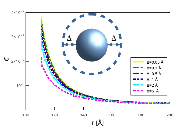
Figure 3: The density profiles of ions for different size $\Delta$ and fixed $l_{g}$=109.9Å. The density is plotted in terms of the number of particles per ų.

III Equilibrium constant for particles interacting via a pair potential

To connect the simulations presented in the previous section with the NP theory we must relate the sticky length with the bulk association constant.

III.1 Neutral pairs

We first consider a general two-component system of sticky spheres. To avoid confusion with previous labels, we designate the “atoms” of each species as X and Y. The interaction between atoms of the same species is

$$u_{xx}(r)=u_{yy}(r)=u_{hs}(r)+u_{sf1}(r),$$ (19)

and between the atoms of different species is

$$u_{xy}(r)=u_{hs}(r)+u_{sf2}(r)+u_{well}(r),$$ (20)

This is the, so called, “physical picture”, in which only atoms exist. Alternatively, we can regard two atoms $X$ and $Y$ in contact to form a molecule $XY$. This corresponds to the “chemical picture”, see Fig. (4) for illustration. In the chemical picture, we have free atoms $X$ and $Y$, and molecules $XY$ which are in “chemical” equilibrium hill ,

$$\ch{X}+\ch{Y}\rightleftharpoons\ch{XY}.$$ (21)

At most two atoms X and Y are permitted to interact via a sticky potential. Without this restriction, one has to account for the presence of triplets XYX, quartets XYXY, and other higher order formations, together with their corresponding chemical reactions.

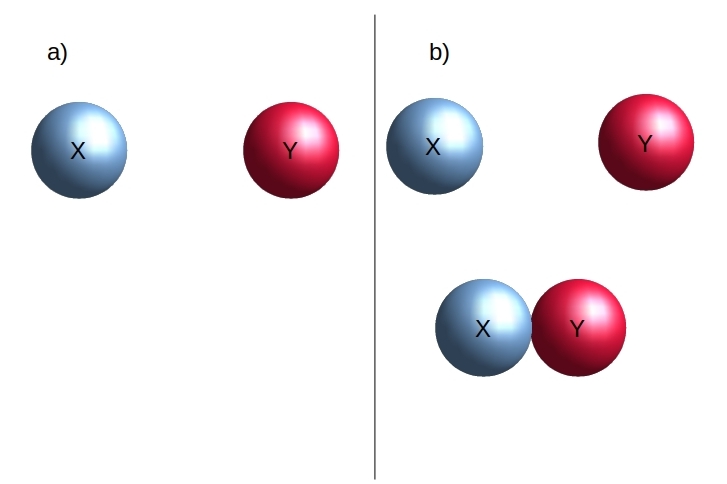
Figure 4: The two representations correspond to a) a physical and b) a chemical interpretation.

To obtain the equilibrium constant for the chemical reaction in Eq. (21) we compare the equations of state calculated using the physical and the chemical pictures. Clearly the osmotic pressure calculated using the two interpretations of the same physical reality has to be same.

Within the physical interpretation, the system is comprised of two types of atoms, X and Y, and the formation of pairs XY is devoid of any special meaning. The virial expansion of the osmotic pressure up to second order in bulk concentration $c_{i}$ is mcquarrie

$$\beta P_{phys}=c_{x}+c_{y}+B_{xx}c_{x}^{2}+B_{yy}c_{y}^{2}+2B_{xy}c_{x}c_{y}+\dots,$$ (22)

where $B_{ij}$ are the second virial coefficients defined as

$$B_{ij}=2\pi\int_{0}^{\infty}\Big{(}1-\mathrm{e}^{-\beta u_{ij}(r)}\Big{)}\,r^{2}dr,$$ (23)

and whose various contributions are

$$~{}~{}~{}~{}~{}~{}~{}~{}~{}~{}~{}~{}B_{xx}=B_{yy}=B_{hs}+B_{sf1},$$

$$~{}~{}~{}~{}~{}~{}~{}~{}~{}~{}~{}~{}B_{xy}=B_{hs}+B_{st}+B_{sf2},$$ (24)

which, after evaluation, become

$$~{}~{}~{}~{}~{}~{}~{}~{}~{}~{}~{}~{}B_{hs}=\frac{2\pi d^{3}}{3},$$

$$~{}~{}~{}~{}~{}~{}~{}~{}~{}~{}~{}~{}B_{st}=-2\pi l_{g}d^{2}e^{-\beta u_{sf2}(d)},$$

$$~{}~{}~{}~{}~{}~{}~{}~{}~{}~{}~{}~{}B_{sf1}=2\pi\int_{d}^{\infty}\Big{(}1-\mathrm{e}^{-\beta u_{sf1}(r)}\Big{)}\,r^{2}dr,$$

$$~{}~{}~{}~{}~{}~{}~{}~{}~{}~{}~{}~{}B_{sf2}=2\pi\int_{d}^{\infty}\Big{(}1-\mathrm{e}^{-\beta u_{sf2}(r)}\Big{)}\,r^{2}dr,$$

(25)

where $B_{st}$ was evaluated using the Boltzmann factor in Eq. (16). Inserting these contributions into the expansion in Eq. (22) yields

$$\beta P_{phys} = c_{x}+c_{y}$$ (26)

$$+ B_{hs}\big{(}c_{x}+c_{y}\big{)}^{2}+B_{sf1}\big{(}c_{x}^{2}+c_{y}^{2}\big{)}+2B_{sf2}c_{x}c_{y}$$

$$+ 2B_{st}c_{x}c_{y}+\dots,$$

where the first line is the ideal-gas contribution, the second line is the second order correction due to hard-core and soft interactions, and the third line is the second order correction due to the sticky potential.

To formulate the equation of state within the chemical picture, we need to define the concentrations of free atoms X, Y, and of molecules XY, designated by the superscript *:

$$~{}~{}~{}~{}~{}~{}~{}~{}~{}~{}~{}~{}~{}~{}~{}~{}~{}~{}~{}~{}~{}~{}~{}c^{*}_{x}=c_{x}-c^{*}_{xy},$$

$$~{}~{}~{}~{}~{}~{}~{}~{}~{}~{}~{}~{}~{}~{}~{}~{}~{}~{}~{}~{}~{}~{}~{}c^{*}_{y}=c_{y}-c^{*}_{xy},$$

$$~{}~{}~{}~{}~{}~{}~{}~{}~{}~{}~{}~{}~{}~{}~{}~{}~{}~{}~{}~{}~{}~{}~{}c^{*}_{xy}=K_{Bulk}{c_{x}^{*}}c_{y}^{*},$$ (27)

where the last equation was obtained using the definition of the equilibrium constant of the reaction in Eq. (21),

$$K_{Bulk}=\frac{c^{*}_{xy}}{c^{*}_{x}c^{*}_{y}},$$ (28)

valid in the dilute limit where activities are approximated by concentrations. To second order in concentrations $c_{i}$, Eq. (27) can be written as

$$~{}~{}~{}~{}~{}~{}~{}~{}~{}~{}~{}~{}~{}~{}~{}~{}c^{*}_{x}=c_{x}-K_{Bulk}{c_{x}}c_{y}+\dots,$$

$$~{}~{}~{}~{}~{}~{}~{}~{}~{}~{}~{}~{}~{}~{}~{}~{}c^{*}_{y}=c_{y}-K_{Bulk}{c_{x}}c_{y}+\dots,$$

$$~{}~{}~{}~{}~{}~{}~{}~{}~{}~{}~{}~{}~{}~{}~{}~{}c^{*}_{xy}=K_{Bulk}{c_{x}}c_{y}+\dots.$$ (29)

In the chemical picture, the interactions between free atoms X and Y do not include sticky interaction,

$$u^{\prime}_{xy}(r)=u_{hs}(r)+u_{sf2}(r).$$

which acts only within a molecule XY. Without the sticky interaction, the modified second virial coefficient in the chemical interpretation is

$$B^{\prime}_{xy}=B_{hs}+B_{sf2}.$$ (30)

The osmotic pressure up to second order in concentrations $c_{i}$ is then

$$\beta P_{chem}=c_{x}^{*}+c_{y}^{*}+c_{xy}^{*}+B_{xx}c_{x}^{*2}+B_{yy}c_{y}^{*2}+2B^{\prime}_{xy}c_{x}^{*}c_{y}^{*}+\dots.$$ (31)

The terms

$$2B_{x,xy}c_{x}^{*}c_{xy}^{*}+2B_{y,xy}c_{y}^{*}c_{xy}^{*}+B_{xy,xy}c_{xy}^{*2},$$ (32)

that are second order in $c_{i}^{*}$ are omitted since, due to $c_{xy}^{*}\approx K_{Bulk}{c_{x}}c_{y}$ in Eq. (29), they are of higher order in $c_{i}$. Using formulas in Eq. (29), and substituting for the coefficients $B_{ij}$, Eq. (31) becomes

$$\beta P_{chem} = c_{x}+c_{y}$$ (33)

$$+ B_{hs}\big{(}c_{x}+c_{y}\big{)}^{2}+B_{sf1}\big{(}c_{x}^{2}+c_{y}^{2}\big{)}+2B_{sf2}c_{x}c_{y}$$

$$- K_{Bulk}c_{x}c_{y}+\dots,$$

Setting $P_{phys}=P_{chem}$, and matching the terms of the same order yields

$$K_{Bulk}=-2B_{st}=4\pi l_{g}{d}^{2}e^{-\beta u_{sf2}(d)},$$ (34)

We note that the above derivation assumes a dilute limit, where the definition of $K_{Bulk}$ in Eq. (28) and the second order expansion of $\beta P$ are valid. The result in Eq. (34), however, is exact for any concentration. This is because the quantity $K_{Bulk}$ itself is independent of concentrations. We simply took advantage of this fact and chose the limit where all the expressions are the simplest.

If we set $u_{fs2}=0$ , the equilibrium constant becomes

$$K_{Bulk}=4\pi l_{g}{d}^{2},$$ (35)

which is appropriate for the pair formation between bases and hydronium ions. On the other hand, as we will see in the following section, Eq. (34) with $u_{sf2}$ corresponding to the Coulomb potential will be appropriate for weak acid-hydronium equilibrium constant.

III.2 Charged pairs

In bulk, acid “molecule” dissociates resulting in a hydronium ion and a corresponding anion:

$$\ch{HA}\rightleftarrows\ch{H^{+}}+\ch{A^{-}},$$ (36)

The thermodynamics of bulk electrolytes, even without covalent bonding between the ions, is complicated by the divergence of the virial expansion due to the long range nature of the Coulomb interaction. Instead a certain class of perturbative diagrams must be summed together to obtain a finite result mcquarrie . This leads to a non-analytic term in the density expansion of the osmotic pressure which scales with electrolyte concentration as $c^{3/2}$. The next order term which scales as $c^{2}$ can be interpreted as the result of Bjerrum anion-cation pair formation. In the case of purely electrostatic interactions, the equilibrium constant for such cluster formation was derived by Ebeling eblingo68 considering the exact density expansion of the equation of state up to $\mathcal{O}\left(c^{5/2}\right)$ Falkenhagen . The Ebeling equilibrium constant is:

$$\begin{split}K_{Eb}=8\pi d^{3}\left\{\frac{1}{12}b^{3}\right.\left[\mathrm{Ei}\left(b\right)-\mathrm{Ei}\left(-b\right)\right]-\frac{1}{3}\cosh{b}-\\ \frac{1}{6}b\sinh{b}-\left.\frac{1}{6}b^{2}\cosh{b}+\frac{1}{3}+\frac{1}{2}b^{2}\right\},\end{split}$$ (37)

where $b=\frac{\lambda_{B}}{d}$. For large values of $b$ (strong coupling limit), the equilibrium constant can be expanded asymptotically to give:

$$K_{Eb}=4\pi a^{3}\frac{\mathrm{e}^{b}}{b}\left(1+\frac{4}{b}+\frac{4\times 5}{b^{2}}+\frac{4\times 5\times 6}{b^{3}}+...\right)\,.$$ (38)

This may be compared with the Bjerrum phenomenological association constant for formation of anion-cation pairs

$$K_{Bj}=4\pi\int_{d}^{R_{Bj}}\mathrm{e}^{\frac{\lambda_{B}}{r}}r^{2}dr,$$ (39)

where $R_{Bj}=\lambda_{B}/2$ is the Bjerrum cutoff. In the strong coupling limit (low temperatures), $K_{Bj}$ is completely insensitive to the precise value of cutoff $R_{Bj}$ levin . Furthermore, the low temperature expansions for $K_{Eb}$ and $K_{Bj}$ are found to be identical levin . One can then interpret the Ebeling equilibrium constant as the analytic continuation of $K_{Bj}$ over the full temperature range. With this observation it becomes easy to obtain the equilibrium constant for sticky electrolytes. In the spirit of Bjerrum, we then write

$$K_{Bulk}=4\pi\int_{d}^{R_{Bj}}\mathrm{e}^{-\beta u_{st}(r)+\frac{\lambda_{B}}{r}}r^{2}dr.$$ (40)

Using Eq.(16) we obtain

$$K_{Bulk}=4\pi\int_{d}^{R_{Bj}}\left[(1+l_{g}\delta(r-d)\right]\mathrm{e}^{\frac{\lambda_{B}}{r}}r^{2}dr\,,$$ (41)

which after integration yields,

$$K_{Bulk}=4\pi d^{2}l_{g}\mathrm{e}^{b}+\int_{d}^{R_{Bj}}\mathrm{e}^{\frac{\lambda_{B}}{r}}r^{2}dr\,.$$ (42)

The validity of the above equation is extended beyond the strong coupling limit by replacing the integral with $K_{Eb}$. In the case of weak acids, large $l_{g}$, the first term will dominate Eq. (42), so that the bulk equilibrium constant for a weak acid can be approximated by

$$K_{Bulk}=4\pi d^{2}l_{g}\mathrm{e}^{b},$$ (43)

which is similar to Eq. (34) of the previous section.

IV Uniformly sticky colloid

To build a theory of charge regularization of colloidal particles we start with the simplest possible model in which the whole of colloidal surface is sticky. Colloidal particle of radius $a$ is placed at the center of a spherical WS cell of radius $R$. The density profiles of ions, then, satisfy the modified Poisson-Boltzmann (mPB) equation:

$$\nabla^{2}\phi(r)=-\frac{4\pi}{\epsilon_{w}}\sigma_{0}\delta(r-a-r_{ion})-\frac{4\pi q}{\epsilon_{w}}\left[c_{\ch{H^{+}}}(r)+c_{+}(r)-c_{-}(r)\right],$$ (44)

where $\sigma_{0}=0$ if the surface groups are basic, and $\sigma_{0}=-N_{sites}q/4\pi(a+r_{ion})^{2}$ if all the groups are acidic. The ionic concentrations are defined as:

$$c_{\ch{H^{+}}}(r)=c_{a}~{}\mathrm{e}^{-\beta\left(u(r)+q\phi(r)\right)}$$ (45)

$$c_{+}(r)=c_{s}~{}\mathrm{e}^{-\beta q\phi(r)}$$ (46)

$$c_{-}(r)=(c_{a}+c_{s})~{}\mathrm{e}^{\beta q\phi(r)},$$ (47)

where $u(r)$ is the sticky potential between the colloidal surface and a hydronium ion, $c_{a}=10^{-pH}$ is the reservoir concentration of acid, and $c_{s}$ is the reservoir concentration of 1:1 salt. We assume that both acid and salt in the reservoir are strong electrolytes and are fully dissociated. Using Eq. 16 we obtain $\mathrm{e}^{-\beta\left(u(r)+q\phi(r)\right)}=(1-l_{g}\delta(r-a-r_{ion}))\mathrm{e}^{-\beta q\phi(r)}$, which means that the surface density of adsorbed hydronium ions is bakhshandeh2019 :

$$\begin{split}\sigma_{su}=qc_{a}l_{g}\mathrm{e}^{-\beta q\phi_{0}},\end{split}$$ (48)

where $\phi_{0}=\phi(a+r_{ion})$. The net surface charge density is then

$$\sigma_{net}=\sigma_{0}+\sigma_{su}.$$ (49)

To calculate the ionic density profiles and the number of condensed hydronium ions we must now solve the PB equation

$$\nabla^{2}\phi(r)=\frac{8\pi q}{\epsilon_{w}}\left(c_{a}+c_{s}\right)\sinh[\beta\phi(r)],$$ (50)

with the boundary conditions $\phi^{\prime}(R)=0$ and $\phi^{\prime}(a+r_{ion})=4\pi\sigma_{net}/\epsilon_{w}$. The calculation can be performed numerically using the 4th order Runge-Kutta, in which the value of the surface potential $\phi(a+r_{ion})=\phi_{0}$ is adjusted based on the Newton-Raphson algorithm to obtain zero electric field at the cell boundary.

In realty, however, the whole of colloidal surface is not uniformly sticky and hydronium ions can only adsorb on special sites jho2012 . We now explicitly consider the modifications that must be made to the above theory in order to account for the discrete nature of adsorption sites.

V Neutral functional groups

We first consider a colloidal particle with $N_{site}$ neutral basic groups (sticky spheres) uniformly distributed on its surface. To simplify the geometry we will map the spherical sticky sites onto circular sticky patches of the same effective contact area. Since both hydronium and the adsorption sites are modeled by spheres of the same diameter $d$, the hard core repulsion between the colloidal surface and the hydronium ion restricts the effective contact area to $2\pi d^{2}$. Therefore, the patch radius must be

$$\begin{split}r_{patch}=\sqrt{2}~{}d,\end{split}$$ (51)

Compared to the situation discussed in the previous section in which the whole of colloidal surface was sticky, the effective area on which hydronium ions can become adsorbed is significantly reduced in the case of discrete adsorption sites bakhshandeh2019 . Nevertheless, we can still use the same approach as in Section IV, if the sticky length is rescaled as $l_{g}^{eff}=l_{g}\alpha_{eff}$, to account for the reduced adsorption area, where

$$\alpha_{eff}=\frac{N_{site}^{act}\pi r_{patch}^{2}}{4\pi(a+r_{ion})^{2}},$$ (52)

is the fraction of the surface area occupied by the active sticky patches. Note that if hydronium is adsorbed to a patch, this patch becomes inactive, preventing more than one hydronium ion from being adsorbed. The number of adsorbed hydronium ion is given by Eq. (48) with $l_{g}$ replaced by $l_{g}^{eff}$. As the process of adsorption progresses, the number of active sites decreases in such a way as

$$N_{site}^{act}=N_{site}-4\pi(a+r_{ion})^{2}c_{a}l_{g}^{eff}~{}\mathrm{e}^{-\beta\phi_{0}},$$ (53)

resulting in a self-consistent equation for $l_{g}^{eff}$ . Solving Eqs. (52) and (53), the effective sticky length is found to be

$$l_{g}^{eff}=\frac{l_{g}N_{site}r_{patch}^{2}}{4(a+r_{ion})^{2}\left(1+l_{g}c_{a}\mathrm{e}^{-\beta\phi_{0}}\pi r_{patch}^{2}\right)}.$$ (54)

The effective surface charge density which must be used as the boundary condition for PB equation is then

$$\sigma_{eff}=qc_{a}l_{g}^{eff}\mathrm{e}^{-\beta\phi_{0}}=\frac{qK_{Surf}N_{site}c_{a}\mathrm{e}^{-\beta\phi_{0}}}{4\pi(a+r_{ion})^{2}\left(1+K_{Surf}c_{a}\mathrm{e}^{-\beta\phi_{0}}\right)},$$ (55)

where $K_{Surf}=2\pi l_{g}d^{2}=K_{Bulk}/2$, where the bulk association constant is the same as in Eq. 35.

We stress again that the bulk equilibrium constant $K_{Bulk}$ is exact for the model of sticky hard spheres and does not depend on the density of the reactants. The higher order terms of the virial expansion, however, will modify the activity coefficients, so that in the law of mass action the concentrations will have to be replaced by the activities. Nevertheless, since the PB equation does not take into account ionic correlations, to remain consistent, the activity coefficients must also be set to unity. Solving Eq. 50, with the boundary conditions $\phi^{\prime}(R)=0$ and $\phi^{\prime}(a+r_{ion})=4\pi\sigma_{net}/\epsilon_{w}$ we are able to obtain the density profile of ions around the colloidal particle.

To explore the range of validity of the theory we will compare it with the results of Monte Carlo simulations. We first consider colloidal particles with $300$ and $600$ active neutral basic sites and concentration of HCl set to $50$ mM. In Figs. 5 and  6 we show the comparison between the simulation data, NP theory, and the present work, For these parameters the difference between the new theory and the NP approach is not very large, nevertheless it is clear that the simulation results are in a much better agreement with the theory developed in the present paper. The figures show that the density of free hydronium ions decreases near the colloidal surface. This is not surprising, since once some of the hydroniums have adsorbed to the neutral basic groups, colloidal surface becomes positively charged and repels other cations. A more curious behavior is found for the anion Cl-, the concentration of which shows a peak close to the surface, but then diminishes on further approach. The reason for this is that anions prefer to stay close to the adsorbed cations H+, which in turn want to minimize the repulsive electrostatic energy between themselves, as well as to maximize entropy. This favors the hydronium ions to be located at about $~{}3~{}r_{ion}$ from the colloidal surface. This is precisely the position of the peak found in the density profile of anions. This fine detail, however, is beyond the scope of the present theory. Nevertheless the fact that the density profiles away from colloidal surface are perfectly described by the present theory implies that the prediction for the total number of adsorbed hydronium ions is correct, in spite of the fine structure of ionic density profiles near the surface.

Figure 5: Density profiles of hydronium and Cl- measured in particles per ų . Symbols are the simulation data and solid (green) and dashed (blue) lines are the predictions of the NP theory and of the theory developed in the present work, respectively. The parameters are $a=100$ Å, $R=200$ Å, and $l_{g}=109.97$Å. The colloidal particle has $300$ neutral basic sites on its surface. The concentration of HCl is $50$ mM. a)Density profile of Cl- and b) Density profile of hydronium.

Figure 6: Density profiles of hydronium and Cl- measured in particles per ų . Symbols are the simulation data and solid (green) and dashed (blue) lines are the predictions of the NP theory and of the theory developed in the present work, respectively. The parameters are $a=100$ Å, $R=200$ Å, and $l_{g}=109.97$Å. The colloidal particle has $600$ basic sites on its surface. The concentration of HCl is $50$ mM. a)Density profile of Cl- and b) Density profile of hydronium.

We next consider the effect of 1:1 salt on the charge regulation. We study a colloidal particle with $200$ basic sites in the presence of HCl and NaCl, both at concentration $10$ mM. We assume that both acid and salt are completely ionized. The results of the theory and simulations are shown in Fig. 7.

Figure 7: Density profiles of hydronium, Cl-, and Na+ measured in particles per ų . Symbols are the simulation data and solid (green) and dashed (blue) lines are the predictions of the NP theory and of the theory developed in the present work, respectively. The parameters are $a=100$ Å, $R=200$ Å, and $l_{g}=109.97$Å. The colloidal particle has $200$ basic sites on its surface. The concentration of HCl and NaCl is $10$ mM. The density C is in units of particles per ų.

Once again we see a very good agreement between the present theory and the MCs simulations.

In experiments, Zeta potential is more easily available than the effective charge. Definition of Zeta potential, however, requires knowledge of the position of the slip plain. Nevertheless we expect that Zeta potential will behave similarly to the electrostatic contact surface potential. In Figs. 8 and 9 we show the behavior of the surface potential and the effective charge $Z_{eff}$ in unit of charge $q$ as a function of pH, for the present theory and NP theory, respectively and in Fig 10, the behavior of the two as a function of salt concentration. We observe that addition of 1:1 electrolyte diminishes the contact potential. This, in turn, lowers the electrostatic energy penalty for bringing hydronium ions to colloidal surface, thus favoring their association with the active sites. Indeed, Fig 10b shows that the effective charge of colloidal particle increases with increasing salt concentration.

Figure 8: Contact potential as a function of pH for the present theory and NP theory, respectively. The colloidal particle has $300$ basic functional group on it surface. The parameters are $a=100$ Å, $R=200$ Å, and $l_{g}=109.97$Å. There is no added salt.

Figure 9: Effective charge of colloidal particle in unit of $q$ as a function of pH for the present theory and NP theory, respectively. The colloidal particle has $300$ basic active functional group on it surface. The parameters are $a=100$ Å, $R=200$ Å, and $l_{g}=109.97$Å. There is no added salt.

Figure 10: (a) Contact potential and (b) the effect charge of colloidal particle in unit of $q$ as a function of salt concentration $c_{s}$ (M) for different pH. The colloidal particle has $300$ basic functional group. The parameters are $a=100$ Å, $R=200$ Å, and $l_{g}=109.97$Å.

VI Charged functional groups

We next consider a colloidal particle with $N_{site}$ acidic surface groups each carrying a charge $-q$. If all the groups would be ionized, the particle would acquire a net charge $Q_{0}=-N_{site}q$. The chemical equilibrium between hydronium and acid groups, however, reduces this value to $Q_{eff}=Q_{0}+Q_{con}$, where

$$Q_{con}=4\pi(a+r_{ion})^{2}qc_{a}l_{g}^{eff}\mathrm{e}^{-\beta q\varphi_{0}}$$ (56)

is the number of associated hydronium ion and $\varphi_{0}$ is the potential of mean force (PMF) — the work required to bring an ion from the bulk to contact with one of the acidic groups. The PMF can be separated into a mean-field electrostatic potential $\phi_{0}$ and a contribution from the discrete nature of surface charge groups $\mu^{qq}_{c}$,

$$\varphi_{0}=\phi_{0}+\mu^{qq}_{c}\,.$$ (57)

The value of $l_{g}^{eff}$ is given by Eq. (54) with the mean-field potential replaced by the PMF, $\phi_{0}\rightarrow\varphi_{0}$. The effective surface charge density then reduces to

$$\sigma_{eff}=-\frac{N_{site}q}{4\pi\left(a+r_{ion}\right)^{2}}+\frac{qK_{Surf}^{a}N_{site}c_{a}\mathrm{e}^{-\beta\phi_{0}}}{4\pi(a+r_{ion})^{2}\left(1+K_{Surf}^{a}c_{a}\mathrm{e}^{-\beta\phi_{0}}\right)}$$ (58)

where

$$K_{Surf}^{a}=\frac{K_{Bulk}^{a}}{2}\mathrm{e}^{-b-\beta\mu^{qq}_{c}},$$ (59)

and the bulk acid association constant $K_{Bulk}^{a}$ is given by Eq. (43). The term $\mathrm{e}^{-b}$ in Eq. 59 discounts the direct Coulomb interaction between the hydronium ion and its adsorption site, which is already accounted for in the $\mu^{qq}_{c}$.

VII The effect of discrete charges

It is well known that the PB equation is very accurate for systems containing only 1:1 electrolyte. The mean-field nature of this equation is manifested by the complete neglect of ionic correlations, which are found to be small for aqueous solutions of monovalent ions levin . However, in the case of acidic groups, hydronium ions will condense directly onto charged sites and discrete nature of hydronium ions and surface sites can not be neglected for the associated ions. The free ions, however, can still be treated at the mean-field level.

To account for the discrete nature of surface groups, we add and subtract a uniform neutralizing background to the colloidal surface. The negative of the background can be combined with the mean-field electrostatic potential produced by the ions to yield the total mean-field electrostatic potential $\phi(r)$. The potential produced by the discrete surface charge and their neutralizing background, on the other hand, correspond to $\mu^{qq}_{c}$ defined in Eq.(57). To calculate $\mu^{qq}_{c}$ we will ignore the curvature of the colloidal surface. Furthermore, we will suppose that the adsorption sites are uniformly distributed, forming a triangular lattice of spacing $L$.

We start by calculating the electrostatic potential produced by an infinite planar triangular array of charges, see Fig. 11. This potential must satisfy the Poisson equation

$$\nabla^{2}G(\boldsymbol{r})=-\frac{4\pi q}{\epsilon_{w}}\sum_{n,m}\delta(z)\delta(\boldsymbol{\rho}-n\boldsymbol{a}_{1}-m\boldsymbol{a}_{2}),$$ (60)

Figure 11: The triangular lattice used to evaluate $\mu^{qq}_{c}$ and $\mu^{qq}_{n}$.

where $z$ and $\boldsymbol{\rho}=x\boldsymbol{\hat{x}}+y\boldsymbol{\hat{y}}$ are the transverse and longitudinal directions, respectively, and the lattice vectors are given by

$$\begin{split}\boldsymbol{a}_{1}=L~{}\boldsymbol{\hat{x}},\\ \boldsymbol{a}_{2}=\frac{1}{2}L~{}\boldsymbol{\hat{x}}+\frac{\sqrt{3}}{2}L\boldsymbol{\hat{y}}.\end{split}$$ (61)

The area of the unit cell of triangular lattice is

$$\begin{split}\left|\gamma\right|=\left|\boldsymbol{a}_{1}\times\boldsymbol{a}_{2}\right|=\frac{\sqrt{3}}{2}L^{2}\end{split}$$ (62)

The reciprocal lattice vectors $\boldsymbol{b}_{i}$ are defined as $\boldsymbol{a}_{j}\cdot\boldsymbol{b}_{j}=2\pi\delta_{ij}$, and are given by

$$\begin{split}\boldsymbol{b}_{1}=\frac{2\pi}{d}\left(\boldsymbol{\hat{x}}-\frac{\boldsymbol{\hat{y}}}{\sqrt{3}}\right).\\ \boldsymbol{b}_{2}=\frac{2\pi}{d}\left(\frac{2\boldsymbol{\hat{y}}}{\sqrt{3}}\right).\end{split}$$ (63)

The periodic delta function can be written as

$$\begin{split}\sum_{n,m}\delta(\boldsymbol{\rho}-n\boldsymbol{a}_{1}-m\boldsymbol{a}_{2})=\\ \frac{1}{\gamma}\sum_{n,m}\mathrm{e}^{i\boldsymbol{b}_{1}\cdot\boldsymbol{\rho}n+i\boldsymbol{b}_{2}\cdot\boldsymbol{\rho}m}\end{split}$$ (64)

and the Green function as SaGi17

$$\begin{split}G(\boldsymbol{r})=\frac{1}{\gamma}\sum_{n,m}g_{n,m}(z)\mathrm{e}^{i\boldsymbol{b}_{1}\cdot\boldsymbol{\rho}n+i\boldsymbol{b}_{2}\cdot\boldsymbol{\rho}m},\end{split}$$ (65)

where $g_{n,m}(z)$ is a function of $z$ coordinate only. Substituting Eq. (65) into Eq. (60) we obtain

$$\begin{split}\frac{\partial^{2}g_{n,m}(z)}{\partial z^{2}}-k^{2}g_{n,m}(z)=-\frac{4\pi q}{\epsilon_{w}}\delta(z),\\ k=\sqrt{\frac{4\pi^{2}}{L^{2}}\left(n^{2}+\left(\frac{2m}{\sqrt{3}}-\frac{n}{\sqrt{3}}\right)^{2}\right)},\end{split}$$ (66)

which has a solution of the form

$$g_{n,m}(z)=\begin{cases}A~{}\mathrm{e}^{-kz},&z>0,\\ A~{}\mathrm{e}^{kz},&z<0,\end{cases}$$ (67)

Integrating Eq. (66) once, we see that the derivative of $g(z)$ is discontinuous at $z=0$ with

$$g^{\prime}_{n,m}(0^{+})-g^{\prime}_{n,m}(0^{-})=-\frac{4\pi q}{\epsilon_{w}},$$ (68)

from which we determine $A=2\pi q/\epsilon_{w}k$,. The Green function can then be written as

$$\begin{split}G(\boldsymbol{r})=\frac{2\pi q}{\gamma\epsilon_{w}}\sum_{n=-\infty}^{n=\infty}\sum_{m=-\infty}^{m=\infty}\\ \frac{\mathrm{e}^{-k\left|z\right|}}{k}\cos{\frac{2\pi}{L}\left(nx+\frac{1}{\sqrt{3}}(2ym-yn)\right)}.\end{split}$$ (69)

The $(n=0,m=0)$ term of $G(\boldsymbol{r})$ diverges. Indeed, if we take the limit $k\rightarrow 0$ of the summation and in Eq. (69) we will obtain an infinite constant and a finite term which grows as $\left|z\right|$. This is nothing more than the potential of a uniformly charged plane. Therefore, if we introduce a neutralizing background, we will cancel precisely this term, eliminating the divergence. The electrostatic potential produced by a triangular array of charges on a neutralizing background is then

$$\begin{split}\bar{G}(\boldsymbol{r})=\frac{2\pi q}{\gamma\epsilon_{w}}\sum_{n=-\infty}^{n=\infty\prime}\sum_{m=-\infty}^{m=\infty\prime}\frac{\mathrm{e}^{-k\left|z\right|}}{k}\\ \cos{\frac{2\pi}{L}\left(nx+\frac{1}{\sqrt{3}}(2ym-yn)\right)},\end{split}$$ (70)

where the prime on the sums indicates that we have removed the term $(n=0,m=0)$. Bringing an ion of opposite charge into contact with one of the adsorption sites then yield

$$\begin{split}\mu^{qq}_{c}=-\frac{2\pi q^{2}}{\gamma\epsilon_{w}}\sum_{n=-\infty}^{n=\infty\prime}\sum_{m=-\infty}^{m=\infty\prime}\frac{\mathrm{e}^{-2kr_{ion}}}{k}.\end{split}$$ (71)

Even if sites are not perfectly ordered on the colloidal surface, we still expect that $\mu^{qq}_{c}$ derived in Eq. (71) will provide a reasonably accurate account of the discreteness effects assuming that the average separation between $Z$ acid sites is such that the area per site is $\gamma=4\pi(a+r_{ion})^{2}/Z$, where $\gamma$ is given by Eq. 62. The average separation between acid groups is then $L=(a+r_{ion})\sqrt{8\pi/\sqrt{3}Z}$

We first consider a colloidal particles with $600$ acid surface groups with $l_{g}=109.97$ Å, in a solution of pH = $2$. The ionic density profiles are presented in Fig. 12. We see that the theory is in excellent agreement with simulations, while NP approach shows significant deviation. Next we consider particles with $300$ charged sites inside an acid solution containing 1:1 salt. Once gain there is a good agreement between theory and simulations, see Fig. 13.

Figure 12: Comparison between the present theory (solid lines), NP theory (dashed lines) and simulations (symbols), for colloidal particles with $Z=600$ and $l_{g}=109.97$Å  functional groups. The densities are in units of particles per ų

Figure 13: Comparison between the present theory (solid lines), NP theory (dashed lines) and simulations (symbols), for colloidal particles with $Z=300$ charged functional group with $l_{g}=109.97$Å. Solution is at pH $=3$ and has $10$mM bulk $1:1$ salt concentration. The densities are in units of particles per ų.

In Fig. 14 we show the behavior of the effective charge and contact potential of colloidal particle as a function of 1:1 salt concentration for different pH values.

Figure 14: Modulus of the effective charge in unit of $q$ and contact potential of colloidal particle as a function of 1:1 salt concentration   $C_{s}$ for different values of pH. The colloidal particle has $300$ charged functional group on it surface. The parameters are $a=100$ Å, $R=200$ Å, and $l_{g}=109.97$Å. The densities are in units of particles per ų

The figure shows that increase of salt concentration leads to increase of the modulus of the effective charge. This, again, is a consequence of electrostatic screening produced by salt on the Coulomb interaction between hydronium ions and the negatively charged adsorption sites — making the association of a hydronium with an active site less energetically favorable. In Fig. 15 we compare the effective charge and contact potential calculated using the present theory and the values predicted by the NP theory, for nanoparticles with $300$ charged groups. As can be seen, neglect of discrete charge effects in the NP theory leads to smaller modulus of the contact potential and of the effective charge. We also note that at large pH the effective charge saturates at the value smaller than the bare charge. This is a consequence of the overall charge neutrality of the colloidal suspension. Even if the reservoir has a very small concentration of acid – large pH, in the absence of other cations inside the suspension, there must be enough hydronium ions to compensate all the colloidal charge. Some of these hydronium ions will then associate with the surface groups, leading to the saturation of the effective colloidal charge.

Figure 15: The modulus of the effective charge in units of $q$ and the contact potential of a nanoparticle as a function of pH in the acid reservoir, predicted by the NP and the present theories. The colloidal particle has $300$ charged functional group on it surface. The parameters are $a=100$ Å, $R=200$ Å, and $l_{g}=109.97$Å. The system is salt-free.

We now perform the same calculation, but in the present of a reservoir with $10$ mM monovalent salt. As can be seen in Fig. 16, in the presence of salt, for high pH both NP and our theory predict that the effective charge approaches the bare charge. This is should be contrasted with the no-salt system. When the system is connected to both the salt and acid reservoirs, at large pH the hydronium ions inside the system are replaced by the salt cations, which then control the overall charge neutrality of the colloidal suspension. Since in our model salt cations do not react with the surface groups, for reservoir at large pH very few hydronium ions will be present inside the suspension. Therefore, all the surface groups will become ionized, and the effective colloidal charge will approach the value of the bare charge.

Figure 16: The modulus of the effective charge in units of $q$ and the contact potential of a nanoparticle as a function of pH in the acid reservoir, predicted by the NP and the present theories. The colloidal particle has $300$ charged functional group on it surface. The suspension is in a contact with a monovalent salt reservoir at concentration of $10$ mM. The parameters are $a=100$ Å, $R=200$ Å, and $l_{g}=109.97$Å.

VIII Mixture of functional groups

As a final example we consider a colloidal particle with a mixture of acidic and basic surface groups. Following the same approach introduced in the previous sections we find that the effective surface charge is

$$\begin{split}\sigma_{eff}=-\frac{N_{acid}q}{4\pi(a+r_{ion})^{2}}+q(l^{eff}_{gc}~{}c_{a}~{}e^{-\beta\varphi_{0}^{c}}+l^{eff}_{gn}~{}c_{a}~{}e^{-\beta\varphi_{0}^{n}}),\\ l_{gc}^{eff}=\frac{l_{gc}~{}N_{acid}~{}r_{patch}^{2}}{4(a+r_{ion})^{2}\left(1+l_{gc}c_{a}\mathrm{e}^{-\beta\varphi_{0}^{c}}\pi r_{patch}^{2}\right)},\\ l_{gn}^{eff}=\frac{l_{gn}~{}N_{base}~{}r_{patch}^{2}}{4(a+r_{ion})^{2}\left(1+l_{gn}c_{a}\mathrm{e}^{-\beta\varphi_{0}^{n}}\pi r_{patch}^{2}\right)},\\ \end{split}$$ (72)

where $N_{acid}$ is the number of acidic groups and $N_{base}=N_{site}-N_{acid}$ is the number of basic groups. The effective sticky length for acidic (charged) and basic (neutral) groups are: $l^{eff}_{gc}$ and $l^{eff}_{gn}$, respectively. The discreteness effects will manifest themselves in different ways for hydronium ions condensing on acidic and basic groups,

$$\begin{split}\beta\varphi_{0}^{c}=\beta\phi_{0}^{c}+\mu^{qq}_{c},\\ \beta\varphi_{0}^{n}=\beta\phi_{0}^{n}+\mu^{qq}_{n},\\ \end{split}$$ (73)

Since the values $\mu^{qq}_{c,n}$ depend only on the electrostatic interaction between the hydronium ion and the charged (acid) sites, the value of $\mu^{qq}_{c}$ will be the same as in Eq. (71), depending only on the average separation between the acidic groups. We will suppose that the basic groups are also uniformly distributed on the colloidal surface on a dual hexagonal lattice with vertexes at the center of each triangle composed of acidic sites. In this case the position of one of the basic groups will be at $x_{0}=d/2$,$y_{0}=\sqrt{3d}/4$. Using Eq. (70) we obtain $\mu^{qq}_{n}$

$$\begin{split}\mu_{n}^{qq}=-\frac{2\pi q^{2}}{\gamma\epsilon_{w}}\sum_{n=-\infty}^{n=\infty\prime}\sum_{m=-\infty}^{m=\infty\prime}\frac{\mathrm{e}^{-2kr_{ion}}}{k}\cos{\pi\left(m+\frac{n}{2}\right)}\end{split}$$ (74)

The effective surface charge density can now be written as

$$\sigma_{eff} = -\frac{N_{acid}~{}q}{4\pi\left(a+r_{ion}\right)^{2}}+\frac{qK_{Surf}^{a}~{}N_{acid}~{}c_{a}\mathrm{e}^{-\beta\phi_{0}}}{4\pi(a+r_{ion})^{2}\left(1+K_{Surf}^{a}c_{a}\mathrm{e}^{-\beta\phi_{0}}\right)}+$$ (75)

$$\frac{qK_{Surf}^{b}N_{base}c_{a}\mathrm{e}^{-\beta\phi_{0}}}{4\pi(a+r_{ion})^{2}\left(1+K_{Surf}^{b}c_{a}\mathrm{e}^{-\beta\phi_{0}}\right)}$$

where

$$K_{Surf}^{a}=\frac{K_{Bulk}^{a}}{2}\mathrm{e}^{-b-\beta\mu^{qq}_{c}},$$ (76)

and

$$K_{Surf}^{b}=\frac{K_{Bulk}^{b}}{2}\mathrm{e}^{-\beta\mu^{qq}_{n}}.$$ (77)

The bulk equilibrium constants for acid and base, $K_{Bulk}^{a}$ and $K_{Bulk}^{b}$, are given by Eqs. (43) and (35), respectively. To test our theory for mixture of basic and acidic surface groups we, once again, compare it with MC simulations. We consider a colloidal particle with $500$ adsorption sites with different number of acidic groups $N_{acid}$. The sticky lengths — $l_{gc}$ and $l_{gn}$ — are $109.97$ and $1099.7$, respectively. These values correspond to the equilibrium constants $K_{eq}=$ $0.012$ and $0.00125$ M, respectively. The concentration of strong acid, HCl, in the reservoir is fixed at $10$ mM. We note that as the value of the sticky length $l_{g}$ increases, it becomes progressively more difficult to equilibrate the simulations. For this reason we have chosen values of $l_{g}$ that are not too large. This, however, has no implication for the theory, which remains valid for arbitrary values of $l_{g}$ and $K_{eq}$.

Since the theory is completely general, the values of $l_{g}$ are arbitrarily and one can, in practice, choose the depth and the width of the sticky potential and calculated the sticky length. There is, however, an additional constraint. The equilibration of the simulations becomes progressively more difficult with increase of sticky length. To have a good test of the theory we, therefore, need to chose sufficiently large sticky length to have a significant association of hydronium ions with the adsorption sites, while keeping a reasonable equilibration CPU time. Furthermore, to better test the validity of the theory, we should choose very different sticky lengths for acid and base sites. This is the reason for a factor of $10$ difference between the values of $l_{g}$ of acidic and basic groups. In Table. 1 we show the values of $\mu^{qq}_{c}$ and $\mu^{qq}_{n}$, calculated using Eqs. (71) and (74), respectively – for a colloidal particle with the total of $N_{site}=500$ adsorption sites, $N_{acid}$ of which are acidic (charged) and the rest are basic.

$N_{acid}$	500	450	300	200	50
$\mu^{qq}_{c}$	-0.6278	-0.6653	-0.8073	-0.94227	-1.31329
$\mu^{qq}_{n}$	———	0.14311	0.1519	0.1529	0.119273

Table 1: Different values of $\mu^{qq}_{c}$ and$\mu^{qq}_{n}$ for mixture of charged sites. The total number of adsorption sites is $500$

Fig. 17 shows that for small number of basic sites, the theory remains very accurate. This is also the case if the number of basic sites is significantly larger than the number of acidic sites. The worst agreement is found when $N_{acid}\approx N_{base}$ in which case the surface of colloid becomes strongly heterogeneous, with positive, negative, and neutral domains present, leading to the breakdown of assumptions used to calculate $\mu^{qq}_{c,n}$.

From the obtained results, we conclude that the theory works very well if colloidal particle has either basic or acidic adsorption sites. The discrete charge effects are embedded in the $\mu^{qq}_{c}$ and $\mu^{qq}_{n}$, which are calculated using a regular arrangement of adsorption sites, even though in the simulations the sites are randomly distributed. If the number of acid and base sites is approximately equal, then after the adsorption, we will end up with large domains composed of $-1$,$0$,$+1$ charges, and our assumptions for calculating $\mu^{qq}_{c}$ and $\mu^{qq}_{n}$ will break down. Nevertheless the theory is found to work quite well, as long as the number of acidic and basic sites is not the same. Addition of salt to the system results in even better agreement between theory and simulations. Therefore, the salt free case, provides the most stringent test of the theoretical approach.

Figure 17: Density profile of ions around colloidal particle with different number of charged and neutral functional groups. The total number of sites is $N_{site}=500$, the of the reservoir is pH = $2$ and there is no additional salt. Symbols are the results of MC simulations and the lines are predictions of the theory. The densities are in units of particles per ų

IX Conclusion

In this work, we used a sticky sphere model to mimic chemical reaction on a colloidal surface. Within our theory, the discrete charge effects come only from acid surface sites, since ions are treated at the mean field Poisson-Boltzmann level. This is the reason why the surface equilibrium constant is dependent only on the value of $\mu^{qq}$. In the previous work we studied colloidal particles with only acidic surface groups bakhshandeh2019 . In that approach we used one component plasma model (OCP), to account for the electrostatic corrections due to discrete surface groups. While the approach in Ref. bakhshandeh2019 was sufficiently accurate for colloidal particles with only acidic groups, the OCP does not take into account ionic radius, which prevented us from extending this approach to colloidal particles with a mixture of acidic and basic surface groups. In the present study, we have developed a completely different method to account for discrete surface effects using periodic Green functions. The fact that theory works well even for very small nanoparticles of $10$ nm radius shows the robustness of our approach.

The microscopic model presented in the paper permits us to study the same chemical reaction taking place in bulk and at the interface. In the case of neutral basic surface groups our theory reduces to the NP approach with the bulk equilibrium constant replaced by the surface equilibrium constant,

$$K_{Surf}^{b}\to\frac{1}{2}K_{Bulk}^{b}.$$ (78)

The difference between surface and bulk equilibrium constants is a consequence of steric repulsion, which restricts the overall surface area of the adsorption sites available for interaction with hydronium ions.

For colloidal particles with acidic surface groups the situation is significantly more complex. In this case our theory reduces to the NP approach with an effective surface equilibrium constant only for weak acidic groups. For such systems we find the surface equilibrium constant to be

$$K_{Surf}^{a}=\frac{K_{Bulk}^{a}}{2}\mathrm{e}^{-b-\beta\mu^{qq}_{c}},$$ (79)

where $\mu^{qq}_{c}$ accounts for the discreteness of surface charge. For colloidal particles with a mixture of acidic and basic surface groups, the respective surface equilibrium constants are given by Eqs. (76) and (77).

It is important to stress that Eqs. (78) and (79) are not universal, and in general will depend on the details of the system. These details may include molecular geometry, modified electronic structure of surface functional groups, water structure, etc. Nevertheless the model of sticky adsorption sites demonstrates that there is a mapping between the bulk and the surface equilibrium constants which allows one to use the Poisson-Boltzmann framework to accurately account for the charge regulation in colloidal systems. Any deviations from experiment can therefore be attributed to the shortfall of the model and not to the theoretical method used to solve it.

In this work our primary goal was to explore the extent of validity of the mean-field NP approach by applying it to an exactly solvable model. Clearly the microscopic model that we used for spherically symmetric hydronium, uniform dielectric water, sticky interactions for covalent binding, etc., is a very rough approximation to the physical reality. The advantage is that we can solve this model exactly using computer simulations. Applying the NP approach to the same model we can then test the extent of validity of the mean-field approximations. We should stress that the NP theory does not give us any information whatsoever about the surface equilibrium constant and assumes it to be the same as the bulk association constant. We find, on the there hand, that sticky interactions result in a breakdown of the mean-field approximations. Surprisingly, however, we find that all the discreteness effects can be included in a renormalized surface association constant, which our theory predicts explicitly. For our microscopic model the correlations and steric effects lead to lower surface association constant $K_{Surf}$, compared to the bulk association constant for the same acid or base, $K_{Bulk}$. This means that fewer hydronium ions will bind to surface groups, implying that surface p$K_{a}$ will be smaller than bulk p$K_{a}$. Within the present model, there are two contributions which account for the decrease of the association constant at the surface. First, is the steric repulsion from the colloidal surface, which diminishes the access of hydronium to acid and base groups. Within our model the accessible area for the charge transfer reaction is lowered by a factor of two, which accounts for the factor of $1/2$ which appears in the surface binding constant. The second contribution comes from the discrete nature of surface charged groups, which we also find to lower the effective binding constant. On the other hand, the experiments indicate that the surface binding constant, $K_{Surf}$, that one needs to use in the NP theory is actually larger than $K_{Bulk}$. This means that the surface p$K_{a}$ is larger than the p$K_{a}$ of the bulk acid Behrens . Since our model already takes into account all the steric and electrostatic effects at the dielectric continuum level, we must conclude that in order to account for the experimental results we must included additional effects into the model, such dielectric discontinuity across the colloidal structure, water ordering, quantum nature of proton transfer, etc. The approach that we have developed should allow us to explore these additional effects in order to understand the mechanisms that lead to the increase of p$K_{a}$ at colloidal surface. This will be the subject of the future work.

X ACKNOWLEDGMENT

This work was partially supported by the CNPq.

References

- (1) C. Rønne, L. Thrane, P.-O. Åstrand, A. Wallqvist, K. V. Mikkelsen, and S. R. Keiding, “Investigation of the temperature dependence of dielectric relaxation in liquid water by thz reflection spectroscopy and molecular dynamics simulation,” The Journal of Chemical Physics, vol. 107, no. 14, pp. 5319–5331, 1997.
- (2) D. Andelman, “Chapter 12 - electrostatic properties of membranes: The poisson-boltzmann theory,” in Structure and Dynamics of Membranes (R. Lipowsky and E. Sackmann, eds.), vol. 1 of Handbook of Biological Physics, pp. 603 – 642, North-Holland, 1995.
- (3) R. Messina, “Electrostatics in soft matter,” Journal of Physics: Condensed Matter, vol. 21, p. 113102, feb 2009.
- (4) A. Abrashkin, D. Andelman, and H. Orland, “Dipolar poisson-boltzmann equation: Ions and dipoles close to charge interfaces,” Phys. Rev. Lett., vol. 99, p. 077801, Aug 2007.
- (5) Y. Levin, “Electrostatic correlations: from plasma to biology,” Reports on progress in physics, vol. 65, no. 11, p. 1577, 2002.
- (6) K. Shen and Z.-G. Wang, “Electrostatic correlations and the polyelectrolyte self energy,” The Journal of Chemical Physics, vol. 146, no. 8, p. 084901, 2017.
- (7) A. M. Smith, A. A. Lee, and S. Perkin, “The electrostatic screening length in concentrated electrolytes increases with concentration,” The journal of physical chemistry letters, vol. 7, no. 12, pp. 2157–2163, 2016.
- (8) R. M. Adar, T. Markovich, A. Levy, H. Orland, and D. Andelman, “Dielectric constant of ionic solutions: Combined effects of correlations and excluded volume,” The Journal of Chemical Physics, vol. 149, no. 5, p. 054504, 2018.
- (9) M. I. Bespalova, S. Mahanta, and M. Krishnan, “Single-molecule trapping and measurement in solution,” Current Opinion in Chemical Biology, vol. 51, pp. 113 – 121, 2019. Chemical Genetics and Epigenetics • Molecular Imaging.
- (10) D. Frydel, S. Dietrich, and M. Oettel, “Charge renormalization for effective interactions of colloids at water interfaces,” Phys. Rev. Lett., vol. 99, p. 118302, 2007.
- (11) D. A. Walker, B. Kowalczyk, M. O. de La Cruz, and B. A. Grzybowski, “Electrostatics at the nanoscale,” Nanoscale, vol. 3, no. 4, pp. 1316–1344, 2011.
- (12) S. Alexander, P. Chaikin, P. Grant, G. Morales, P. Pincus, and D. Hone, “Charge renormalization, osmotic pressure, and bulk modulus of colloidal crystals: Theory,” The Journal of Chemical Physics, vol. 80, no. 11, pp. 5776–5781, 1984.
- (13) E. Trizac, L. Bocquet, and M. Aubouy, “Simple approach for charge renormalization in highly charged macroions,” Physical review letters, vol. 89, no. 24, p. 248301, 2002.
- (14) A. Adamson and A. Gast, Chemistry of Surfaces. John Wiley & Sons, New York, NY, USA,, 1997.
- (15) D. Wang, R. J. Nap, I. Lagzi, B. Kowalczyk, S. Han, B. A. Grzybowski, and I. Szleifer, “How and why nanoparticle’s curvature regulates the apparent pka of the coating ligands,” Journal of the American Chemical Society, vol. 133, no. 7, pp. 2192–2197, 2011.
- (16) A. Bakhshandeh, D. Frydel, A. Diehl, and Y. Levin, “Charge regulation of colloidal particles: Theory and simulations,” Physical Review Letters, vol. 123, no. 20, p. 208004, 2019.
- (17) R. Podgornik, “General theory of charge regulation and surface differential capacitance,” The Journal of Chemical Physics, vol. 149, no. 10, p. 104701, 2018.
- (18) D. Frydel, “General theory of charge regulation within the poisson-boltzmann framework: Study of a sticky-charged wall model,” The Journal of Chemical Physics, vol. 150, no. 19, p. 194901, 2019.
- (19) Y. Avni, D. Andelman, and R. Podgornik, “Charge regulation with fixed and mobile charged macromolecules,” Curr Opin Electrochem, vol. 13, pp. 70–77, 2019.
- (20) K. Linderstrøm-Lang, “On the ionization of proteins,” CR Trav. Lab. Carlsberg, vol. 15, no. 7, pp. 1–29, 1924.
- (21) A. Majee, M. Bier, R. Blossey, and R. Podgornik, “Charge regulation radically modifies electrostatics in membrane stacks,” Physical Review E, vol. 100, no. 5, p. 050601, 2019.
- (22) Y. Avni, T. Markovich, R. Podgornik, and D. Andelman, “Charge regulating macro-ions in salt solutions: screening properties and electrostatic interactions,” Soft Matter, vol. 14, pp. 6058–6069, 2018.
- (23) D. Chan, J. PerTam, L. White, and T. Healy, “Regulation of surface potential at amphoteric surfaces during partiele-particle interaction,” J. Chem. Soc. Faraday Trans, vol. 71, pp. 1046–1057, 1975.
- (24) R. Pericet-Camara, G. Papastavrou, S. H. Behrens, and M. Borkovec, “Interaction between charged surfaces on the poisson- boltzmann level: The constant regulation approximation,” The Journal of Physical Chemistry B, vol. 108, no. 50, pp. 19467–19475, 2004.
- (25) H. von Grünberg, “Chemical charge regulation and charge renormalization in concentrated colloidal suspensions,” Journal of Colloid and Interface Science, vol. 219, no. 2, pp. 339 – 344, 1999.
- (26) H. G. Ozcelik and M. Barisik, “Electric charge of nanopatterned silica surfaces,” Physical Chemistry Chemical Physics, vol. 21, no. 14, pp. 7576–7587, 2019.
- (27) A. Lošdorfer Božič and R. Podgornik, “Anomalous multipole expansion: Charge regulation of patchy inhomogeneously charged spherical particles,” The Journal of Chemical Physics, vol. 149, no. 16, p. 163307, 2018.
- (28) F. B. van Swol and D. N. Petsev, “Solution structure effects on the properties of electric double layers with surface charge regulation assessed by density functional theory,” Langmuir, vol. 34, no. 46, pp. 13808–13820, 2018.
- (29) T. Markovich, D. Andelman, and R. Podgornik, “Charge regulation: A generalized boundary condition?,” EPL (Europhysics Letters), vol. 113, p. 26004, jan 2016.
- (30) M. Krishnan, “A simple model for electrical charge in globular macromolecules and linear polyelectrolytes in solution,” The Journal of Chemical Physics, vol. 146, no. 20, p. 205101, 2017.
- (31) M. Krishnan, “Electrostatic free energy for a confined nanoscale object in a fluid,” The Journal of Chemical Physics, vol. 138, no. 11, p. 114906, 2013.
- (32) R. A. Hartvig, M. van de Weert, J. Østergaard, L. Jorgensen, and H. Jensen, “Protein adsorption at charged surfaces: The role of electrostatic interactions and interfacial charge regulation,” Langmuir, vol. 27, no. 6, pp. 2634–2643, 2011.
- (33) D. C. Prieve and E. Ruckenstein, “The surface potential of and double-layer interaction force between surfaces characterized by multiple ionizable groups,” Journal of Theoretical biology, vol. 56, no. 1, pp. 205–228, 1976.
- (34) S. L. Carnie and D. Y. Chan, “Interaction free energy between plates with charge regulation: a linearized model,” Journal of colloid and interface science, vol. 161, no. 1, pp. 260–264, 1993.
- (35) R. Netz, “Charge regulation of weak polyelectrolytes at low-and high-dielectric-constant substrates,” Journal of Physics: Condensed Matter, vol. 15, no. 1, p. S239, 2002.
- (36) A. Majee, M. Bier, and R. Podgornik, “Spontaneous symmetry breaking of charge-regulated surfaces,” Soft Matter, vol. 14, pp. 985–991, 2018.
- (37) J. E. Hallett, D. A. Gillespie, R. M. Richardson, and P. Bartlett, “Charge regulation of nonpolar colloids,” Soft matter, vol. 14, no. 3, pp. 331–343, 2018.
- (38) M. Heinen, T. Palberg, and H. Löwen, “Coupling between bulk- and surface chemistry in suspensions of charged colloids,” The Journal of Chemical Physics, vol. 140, no. 12, p. 124904, 2014.
- (39) C.-Y. Leung, L. C. Palmer, S. Kewalramani, B. Qiao, S. I. Stupp, M. Olvera de la Cruz, and M. J. Bedzyk, “Crystalline polymorphism induced by charge regulation in ionic membranes,” Proceedings of the National Academy of Sciences, vol. 110, no. 41, pp. 16309–16314, 2013.
- (40) G. S. Longo, M. Olvera de la Cruz, and I. Szleifer, “Molecular theory of weak polyelectrolyte gels: The role of ph and salt concentration,” Macromolecules, vol. 44, no. 1, pp. 147–158, 2011.
- (41) R. Zandi, B. Dragnea, A. Travesset, and R. Podgornik, “On virus growth and form,” Physics Reports, 2020.
- (42) D. Roshal, O. Konevtsova, A. L. Božič, R. Podgornik, and S. Rochal, “ph-induced morphological changes of proteinaceous viral shells,” Scientific reports, vol. 9, no. 1, p. 5341, 2019.
- (43) L. Javidpour, A. L. Božič, R. Podgornik, and A. Naji, “Role of metallic core for the stability of virus-like particles in strongly coupled electrostatics,” Scientific reports, vol. 9, no. 1, p. 3884, 2019.
- (44) C. T. Zahler and B. F. Shaw, “What are we missing by not measuring the net charge of proteins?,” Chemistry – A European Journal, vol. 25, no. 32, pp. 7581–7590, 2019.
- (45) A. L. Božič and R. Podgornik, “ph dependence of charge multipole moments in proteins,” Biophysical Journal, vol. 113, no. 7, pp. 1454 – 1465, 2017.
- (46) M. Lund, T. Åkesson, and B. Jönsson, “Enhanced protein adsorption due to charge regulation,” Langmuir, vol. 21, no. 18, pp. 8385–8388, 2005.
- (47) H. Shen and D. D. Frey, “Effect of charge regulation on steric mass-action equilibrium for the ion-exchange adsorption of proteins,” Journal of Chromatography A, vol. 1079, no. 1, pp. 92 – 104, 2005.
- (48) P. M. Biesheuvel and A. Wittemann, “A modified box model including charge regulation for protein adsorption in a spherical polyelectrolyte brush,” The Journal of Physical Chemistry B, vol. 109, no. 9, pp. 4209–4214, 2005.
- (49) N. S. Pujar and A. L. Zydney, “Charge regulation and electrostatic interactions for a spherical particle in a cylindrical pore,” Journal of Colloid and Interface Science, vol. 192, no. 2, pp. 338 – 349, 1997.
- (50) Y. Burak and R. R. Netz, “Charge regulation of interacting weak polyelectrolytes,” The Journal of Physical Chemistry B, vol. 108, no. 15, pp. 4840–4849, 2004.
- (51) R. Kumar, B. G. Sumpter, and S. M. Kilbey, “Charge regulation and local dielectric function in planar polyelectrolyte brushes,” The Journal of Chemical Physics, vol. 136, no. 23, p. 234901, 2012.
- (52) C. Fleck, R. R. Netz, and H. H. von Grünberg, “Poisson–boltzmann theory for membranes with mobile charged lipids and the ph-dependent interaction of a dna molecule with a membrane,” Biophysical Journal, vol. 82, no. 1, pp. 76 – 92, 2002.
- (53) M. Lund and B. Jönsson, “Charge regulation in biomolecular solution,” Quarterly Reviews of Biophysics, vol. 46, pp. 265–281, aug 2013.
- (54) M. L. Grant, “Nonuniform charge effects in protein-protein interactions,” Journal of Physical Chemistry B, vol. 105, pp. 2858–2863, apr 2001.
- (55) A. H. Elcock and J. A. McCammon, “Calculation of weak protein-protein interactions: The pH dependence of the second virial coefficient,” Biophysical Journal, vol. 80, pp. 613–625, feb 2001.
- (56) M. Lund and B. Jönsson, “On the Charge Regulation of Proteins,” Biochemistry, vol. 44, no. 15, pp. 5722–5727, 2005.
- (57) A. C. Mason and J. H. Jensen, “Protein-protein binding is often associated with changes in protonation state,” Proteins: Structure, Function, and Bioinformatics, vol. 71, pp. 81–91, apr 2008.
- (58) B. Aguilar, R. Anandakrishnan, J. Z. Ruscio, and A. V. Onufriev, “Statistics and physical origins of pK and ionization state changes upon protein-ligand binding,” Biophysical Journal, vol. 98, pp. 872–880, mar 2010.
- (59) J. Ståhlberg and B. Jönsson, “Influence off charge regulation in electrostatic interaction chromatography of proteins,” Analytical Chemistry, vol. 68, no. 9, pp. 1536–1544, 1996.
- (60) H. K. Tsao, “Electrostatic interaction of an assemblage of charges with a charged surface: the charge-regulation effect,” Langmuir, vol. 16, pp. 7200–7209, sep 2000.
- (61) A. Kubincová, P. H. Hünenberger, and M. Krishnan, “Interfacial solvation can explain attraction between like-charged objects in aqueous solution,” The Journal of Chemical Physics, vol. 152, no. 10, p. 104713, 2020.
- (62) T. Markovich, D. Andelman, and R. Podgornik, “Complex fluids with mobile charge-regulating macro-ions,” EPL (Europhysics Letters), vol. 120, p. 26001, oct 2017.
- (63) R. Podgornik and V. Parsegian, “An electrostatic-surface stability interpretation of the “hydrophobic” force inferred to occur between mica plates in solutions of soluble surfactants,” Chemical physics, vol. 154, no. 3, pp. 477–483, 1991.
- (64) D. Leckband and J. Israelachvili, “Intermolecular forces in biology,” Quarterly reviews of biophysics, vol. 34, no. 2, pp. 105–267, 2001.
- (65) G. Trefalt, S. H. Behrens, and M. Borkovec, “Charge regulation in the electrical double layer: Ion adsorption and surface interactions,” Langmuir, vol. 32, no. 2, pp. 380–400, 2016.
- (66) P. M. Biesheuvel, M. van der Veen, and W. Norde, “A modified poisson-boltzmann model including charge regulation for the adsorption of ionizable polyelectrolytes to charged interfaces, applied to lysozyme adsorption on silica,” The Journal of Physical Chemistry B, vol. 109, no. 9, pp. 4172–4180, 2005.
- (67) J.-P. Hsu and B.-T. Liu, “Stability of colloidal dispersions: Charge regulation/adsorption model,” Langmuir, vol. 15, no. 16, pp. 5219–5226, 1999.
- (68) J. K. Wolterink, L. Koopal, M. C. Stuart, and W. V. Riemsdijk, “Surface charge regulation upon polyelectrolyte adsorption, hematite, polystyrene sulfonate, surface charge regulation: Theoretical calculations and hematite-poly(styrene sulfonate) system,” Colloids and Surfaces A: Physicochemical and Engineering Aspects, vol. 291, no. 1, pp. 13 – 23, 2006.
- (69) I. Popa, G. Papastavrou, and M. Borkovec, “Charge regulation effects on electrostatic patch-charge attraction induced by adsorbed dendrimers,” Phys. Chem. Chem. Phys., vol. 12, pp. 4863–4871, 2010.
- (70) P. Gong, J. Genzer, and I. Szleifer, “Phase behavior and charge regulation of weak polyelectrolyte grafted layers,” Phys. Rev. Lett., vol. 98, p. 018302, Jan 2007.
- (71) S. H. Behrens and M. Borkovec, “Exact Poisson-Boltzmann solution for the interaction of dissimilar charge-regulating surfaces,” Phys. Rev. E, vol. 60, pp. 7040–7048, Dec 1999.
- (72) J. G. Kirkwood and J. B. Shumaker, “The influence of dipole moment fluctuations on the dielectric increment of proteins in solution,” Proceedings of the National Academy of Sciences of the United States of America, vol. 38, no. 10, p. 855, 1952.
- (73) R. Marcus, “Calculation of thermodynamic properties of polyelectrolytes,” The Journal of Chemical Physics, vol. 23, no. 6, pp. 1057–1068, 1955.
- (74) S. Lifson, “Potentiometric titration, association phenomena, and interaction of neighboring groups in polyelectrolytes,” The Journal of Chemical Physics, vol. 26, no. 4, pp. 727–734, 1957.
- (75) N. Adžić and R. Podgornik, “Field-theoretic description of charge regulation interaction,” The European Physical Journal E, vol. 37, p. 49, Jun 2014.
- (76) A. M. Smith, M. Borkovec, and G. Trefalt, “Forces between solid surfaces in aqueous electrolyte solutions,” Advances in Colloid and Interface Science, vol. 275, p. 102078, 2020.
- (77) C. Safinya and J. Radler, Handbook of Lipid Membranes: Molecular, Functional, and Materials Aspects. Taylor & Francis, 2014.
- (78) B. W. Ninham and V. A. Parsegian, “Electrostatic potential between surfaces bearing ionizable groups in ionic equilibrium with physiologic saline solution,” Journal of Theoretical biology, vol. 31, no. 3, pp. 405–428, 1971.
- (79) D. L. Chapman, “Li. a contribution to the theory of electrocapillarity,” The London, Edinburgh, and Dublin philosophical magazine and journal of science, vol. 25, no. 148, pp. 475–481, 1913.
- (80) M. Gouy, “Sur la constitution de la charge électrique à la surface d’un électrolyte,” Anniue Physique(Paris), vol. 9, pp. 457–468, 1910.
- (81) R. Baxter, “Percus-Yevick equation for hard spheres with surface adhesion,” The Journal of Chemical Physics, vol. 49, no. 6, pp. 2770–2774, 1968.
- (82) D. Frydel, “One-dimensional coulomb system in a sticky wall confinement: Exact results,” Phys. Rev. E, vol. 100, p. 042113, Oct 2019.
- (83) M. A. Miller and D. Frenkel, “Competition of percolation and phase separation in a fluid of adhesive hard spheres,” Phys. Rev. Lett., vol. 90, p. 135702, Apr 2003.
- (84) G. Foffi, C. D. Michele, F. Sciortino, and P. Tartaglia, “Scaling of dynamics with the range of interaction in short-range attractive colloids,” Phys. Rev. Lett., vol. 94, p. 078301, Feb 2005.
- (85) J. N. Herrera and L. Blum, “Sticky electrolyte mixtures in the Percus-Yevick/mean spherical approximation,” The Journal of Chemical Physics, vol. 94, no. 7, pp. 5077–5082, 1991.
- (86) L. Blum, M. L. Rosinberg, and J. P. Badiali, “Contact theorems for models of the sticky electrode,” The Journal of Chemical Physics, vol. 90, no. 2, pp. 1285–1286, 1989.
- (87) D. A. Huckaby and L. Blum, “Exact results for the adsorption of a dense fluid onto a triangular lattice of sticky sites,” The Journal of Chemical Physics, vol. 92, no. 4, pp. 2646–2649, 1990.
- (88) J. A. Greathouse and D. A. McQuarrie, “Conventional hypernetted chain force calculations for charged plates with adsorbing counterions,” Journal of Colloid and Interface Science, vol. 181, no. 1, pp. 319 – 325, 1996.
- (89) J. A. Greathouse and D. A. McQuarrie The Journal of Physical Chemistry, vol. 100, no. 5, pp. 1847–1851, 1996.
- (90) M. S. Wertheim, “Fluids with highly directional attractive forces. IV. Equilibrium polymerization,” Journal of Statistical Physics, vol. 42, pp. 477–492, feb 1986.
- (91) Y. Wang, Y. Wang, D. R. Breed, V. N. Manoharan, L. Feng, A. D. Hollingsworth, M. Weck, and D. J. Pine, “Colloids with valence and specific directional bonding,” Nature, vol. 491, pp. 51–55, nov 2012.
- (92) M. N. Tamashiro, Y. Levin, and M. C. Barbosa, “Donnan equilibrium and the osmotic pressure of charged colloidal lattices,” The European Physical Journal B-Condensed Matter and Complex Systems, vol. 1, no. 3, pp. 337–343, 1998.
- (93) N. Metropolis, A. W. Rosenbluth, M. N. Rosenbluth, A. H. Teller, and E. Teller, “Equation of state calculations by fast computing machines,” The Journal of Chemical Physics, vol. 21, no. 6, pp. 1087–1092, 1953.
- (94) D Frenkel and B Smith, Understanding Molecular Simulation. New York: Academic Press, 1996.
- (95) T. Hill, Statistical Mechanics: Principles and Selected Applications Dover Publications Inc. New York, 1987.
- (96) D. A. McQuarrie, Statistical Mechanics. Harper’s Chemistry Series, New York: HarperCollins Publishing, Inc., 1976.
- (97) W. Ebeling, “Zur theorie der bjerrumschen ionenassoziation in elektrolyten,” Zeitschrift für Physikalische Chemie, vol. 238, no. 1, pp. 400–402, 1968.
- (98) H. Falkenhagen and W. Ebeling, Equilibrium Properties of Ionized Dilute Electrolytes. Academic Press, New York, 1971.
- (99) Y. S. Jho, S. A. Safran, M. In, and P. A. Pincus, “Effect of charge inhomogeneity and mobility on colloid aggregation,” Langmuir, vol. 28, no. 22, pp. 8329–8336, 2012.
- (100) A. P. dos Santos, M. Girotto, and Y. Levin, “Simulations of coulomb systems confined by polarizable surfaces using periodic green functions,” The Journal of Chemical Physics, vol. 147, no. 18, p. 184105, 2017.
- (101) S. H. Behrens, D. I. Christl, R. Emmerzael, P. Schurtenberger, and M. Borkovec, “Charging and aggregation properties of carboxyl latex particles:experiments versus dlvo theory,” Langmuir, vol. 16, no. 6, pp. 2566–2575, 2000.