Thermostat for a relativistic gas
Abstract
In memory of Dietrich Stauffer
Molecular dynamics simulations of a three dimensional relativistic gas with a soft potential are conducted with different interactions and particle masses. For all cases the velocity distribution agrees numerically with the Jüttner distribution. We show how the relativistic gas can be coupled to a thermostat to simulate the canonical ensemble at a given temperature . The behaviour of the thermostat is investigated as a function of the thermal inertia and its appropriate range is determined by evaluating the kinetic energy fluctuations.
I Introduction
The velocity distribution of a gas is classically described by the Maxwell-Boltzmann distribution. However, this distribution does not hold in special relativity as can be seen from the fact that there would be a finite probability for particles to exceed the speed of light. This problem becomes more severe for higher temperatures.
Jüttner generalised the Maxwell-Boltzmann distribution in 1911 to relativistic gases [1]. Maximizing the entropy, he derived the following velocity distribution:
| (1) |
where is the temperature, the Boltzmann constant, the mass of the particles, the number of particles, the Lorentz factor and the speed of light. is a normalising factor. The distribution is isotropic since it only depends on the absolute value of the velocity . It is straightforward to obtain the distribution function of the absolute velocity through integration over the solid angle. One obtains:
| (2) |
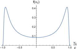
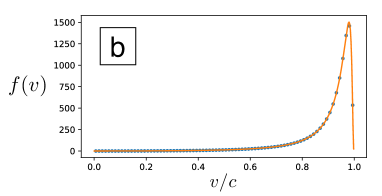
For low temperatures the Jüttner distribution in terms of resembles the Maxwell-Boltzmann distribution but for high temperatures a sharp peak right below the light speed arises reflecting the fact that no particle can exceed the speed of light (see Fig. 1).
In 2007 Cubero et al. conducted simulations in one dimension using collisional dynamics [2]. Their simulation results agree very well with the Jüttner distribution and they could rule out another proposed covariant distribution introduced in Ref. [3]. The same result was found using two dimensional collisional dynamics in a paper by Ghodrat and Montakhab [4]. There a stochastic thermostat was used to simulate the canonical ensemble.
A problem concerning the Jüttner distribution is its non-Lorentz invariance: It depends on the energy of the particle and on whereas a Lorentz invariant distribution would have to be dependent on [5]. To overcome this problem, in Ref. [5] another covariant distribution was proposed that depends on the rapidity instead of the velocities. The rapidity depends on the square of the velocities of the particles relative to each other which is a Lorentz invariant quantity.
Applications of the Jüttner distribution can be found in astrophyics and cosmology, for example in reconstructing the thermal history of the universe [6]. A recent paper investigated a special property of the Jüttner distribution in solid state physics [7]: At high temperatures the Jüttner distribution in terms of a single coordinate exhibits two peaks, one close to and one close to (see fig. 1). This differs from the low temperature regime (and from the Maxwell-Boltzmann distribution) which only broadens when the temperature is increased. In Ref. [7] a critical temperature (with and d the dimension) is found at which the distribution changes from a single peaked function to a double-peaked one. Since at the Dirac point of graphene electrons behave like a relativistic gas, effects of this transition could be measured in graphene when changing the Fermi energy [7].
Here, we will introduce a deterministic relativistic thermostat to simulate the canonical ensemble and verify its properties with three-dimensional simulations using the relativistic equations of motion.
Temperature of a relativistic gas
For a classical ideal gas, the following well-known relation between temperature and kinetic energy holds:
| (3) |
with the particle number. If we include interactions between the particles (i.e. a potential energy ) must be substituted by its time-average for the formula to hold. To see what happens in the case of special relativity, the equipartition theorem can be applied:
where is the Hamiltonian and the momentum of particle .
Using this leads for every particle to
| (4) |
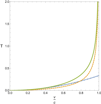
with meaning the square of the norm of the 3-dimensional momentum vector of particle . In the ultrarelativistic limit where this yields the relation
| (5) |
where .
As can be seen in fig. (2) the temperature in special relativity deviates significantly from the classical ideal gas law if the particles approach the speed of light.
II Molecular Dynamics simulation
We simulate a system of particles interacting with a short-ranged soft potential in three dimensions. The trajectories of the particles evolve according to the relativistic equations of motion:
| (6) |
where is the 3-dimensional position of particle and the momentum respectively.
The force is then calculated from . For , the well-known Lennard-Jones potential is used, centered at each particle. It reads in terms of the particle distance
| (7) |
where is the distance between particles and and are parameters.
The accuracy of the method is checked by evaluating the energy
| (8) |
which needs to be conserved. The potential is truncated at . To avoid discontinuities in the potential and its derivative (i.e. the force) at , the potential is further modified by two terms:
| (9) |
Since and its derivative are small quantities at this does not change much the overall shape of the potential. By employing the linked-cell method the complexity can be reduced to [8].
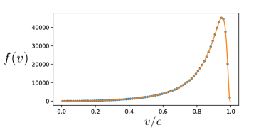
First, only the repelling part of the Lennard-Jones potential (7) proportional to is considered. A histogram is constructed by dividing the range of absolute particle velocities into intervals of equal length. The temperature is calculated using Eq. (4). As can be seen in fig. 3 the obtained data fits the Jüttner distribution very well.
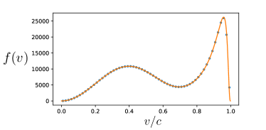
A system of two different sorts of particles with different masses was simulated. In this case both sorts of particles should equilibrate to the same temperature. The theoretical distribution is the sum of two Jüttner distributions for different masses but at the same temperature and normalised with the corresponding particle numbers and :
| (10) |
As can be seen in fig. 4 the particles are indeed fitted well with the sum of two Jüttner distributions at the same temperature according to Eq. (10).
Also a system was considered where the masses of the particles are randomly sampled from a Gaussian distribution . In this case the theoretical Jüttner distribution is a convolution
| (11) |
with being the Jüttner distribution of particles with mass . And also in this case the velocity distribution is well-fitted by the Jüttner distribution of Eq. (11).
III Relativistic thermostat
Because the Hamiltonian equations of motion conserve the energy, the molecular dynamics simulations of the previous chapter simulate the microcanonical statistical ensemble which is defined through constant total energy. Such a system is closed in the sense that there is no energy exchange with an environment. This situation is described by the microcanonical partition function
| (12) |
It is however more natural to allow the system to interact with its environment since experiments are normally conducted at constant temperature and not at constant energy [9]. This situation is statistically described by the canonical ensemble. Here, the system is coupled to an infinite heat bath at a constant temperature which allows the system the exchange of energy. The canonical partition function is:
| (13) |
The temperature of the system can be controlled using a thermostat.
Relativistic simulations with a stochastic thermostat have been conducted in Ref. [4]. A thermostat that is both deterministic and samples from the canonical ensemble is the Nosé-Hoover method [9]. Here a new degree of freedom is introduced that represents the heat bath by adding a term proportional to to the Hamiltonian. After applying Hamilton’s equations of motion, a time transformation needs to be done in order to arrive at the equations in real time which makes the system non-Hamiltonian. This gives rise to a friction parameter in the equations of motion for the momenta.
| (14) |
Here we use the Nosé-Poincaré formalism proposed in Ref. [10] in which the Hamiltonian does not require a time transformation and the usual equations of motion and are directly valid. According to this formalism a new Hamiltonian is introduced:
| (15) |
is the original relativistic Hamiltonian (Eq. 8) but as in the original Nosé-Hoover method the momenta are rescaled by a factor of . The next two terms are responsible for the dynamics of the variable such that the canonical distribution is correctly sampled. is the conjugate momentum of the heat bath. The constant is chosen such that is zero at zero temperature. Finally, the Hamiltonian is multiplied by such that the equations of motion are obtained in real-time.
The Nosé-Poincaré thermostat applied to the relativistic Hamiltonian of Eq. 8 yields:
| (16) |
We will now show that the microcanonical partition function of this extended Hamiltonian is equivalent to the canonical partition function for the relativistic Hamiltonian:
Introducing the substitution and using the properties of the -function yields:
Up to the constant factor from the last integral the canonical distribution function is obtained as we wanted to show. The equations of motion are derived in the usual way through Hamilton’s equations:
After reapplying the transformation they take the following form:
| (17) | ||||
| (18) | ||||
| (19) |
| (20) | ||||
Equation (17) is just the usual relativistic momentum-velocity relation. Eq. (18) is of the form of Eq. (14).
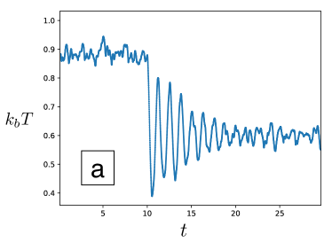
In Fig. 5a the behaviour of the instantaneous temperature (measured by evaluating Eq. (4)) of a system coupled to such a thermostat is shown. The simulation was conducted with particles. Here we did not simulate larger systems, because we want to study in the following statistical fluctuations. The system first had temperature and at time a different temperature was applied to the thermostat. In Fig. 5b we see that the correct Jüttner distribution of the particle velocities is obtained.
The behaviour of the thermostat depends on the choice of the thermal inertia . As can be seen from Eqs. (18), (19) and (20), the thermostat provides a feedback mechanism to control the temperature: If the temperature, represented by the first term of the right hand side in Eq. (20) deviates from the chosen temperature, changes its value and thus following Eq. (18) slows down or speeds up the particles. If is small the ”friction” term in Eq. (18) proportional to changes fast and thus the feedback mechanism is very sensitive. On the other hand, if is very large, the effect of the thermostat disappears.
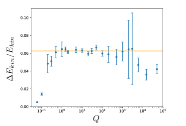
A good choice of is characterised by the fact that canonical energy fluctuations are obtained [11]. The theoretical fluctuations in the canonical ensemble are estimated by calculating . The relative fluctuations should be proportional to where is the number of particles. The behaviour of the kinetic energy fluctuations for a simulation with and is shown in fig. 6. The error bars represent the standard deviation.
In Ref. [12] the effects of different for a classical Nosé-Hoover thermostat were analyzed: If is set correctly, the thermostat couples to the particle motion and the system samples the canonical distribution. However, if the value of is too small or too large the variable oscillates periodically (with quick oscillations if is too small and slow oscillations if is too large). For very high one actually simulates the microcanonical ensemble [12].
For the thermostatted relativistic system a very similar result as in Ref. [12] is obtained. In a medium range of , the canonical fluctuations are reproduced (represented by the orange line in fig. 6); if exceeds this range, the variance of the fluctuations increases and for very large the fluctuations become smaller. If is chosen very small, the kinetic energy fluctuations also become smaller, however the kinetic energy oscillates with a high frequency. In fig. 6 canonical energy fluctuations are observed for .
For small values of Nosé approximated the oscillations of the thermostat with a harmonic oscillator [11]. With a similar procedure this can also be done for the relativistic thermostat: Starting from Eqs. (18) and (19), it is assumed that the motion of the particles is dominated by the thermostat. So we can neglect the dependence of the force , so that all now have the same equation of motion and thus we omit the index and and write . This yields:
| (21) |
Eq. (20) becomes:
| (22) |
and are then linearly approximated around an equilibrium (time-independent) solution and . The zero order solution is
| (23) | ||||
| (24) |
The first order solution yields:
| (25) | ||||
| (26) |
Taking the derivative of Eq. (26) and inserting it in Eq. (25) yields (using Eq. (23)):
| (27) |
which is the equation for a harmonic oscillator from which the frequency can be inferred:
| (28) |
Because of Eq. (26) oscillates with the same frequency.
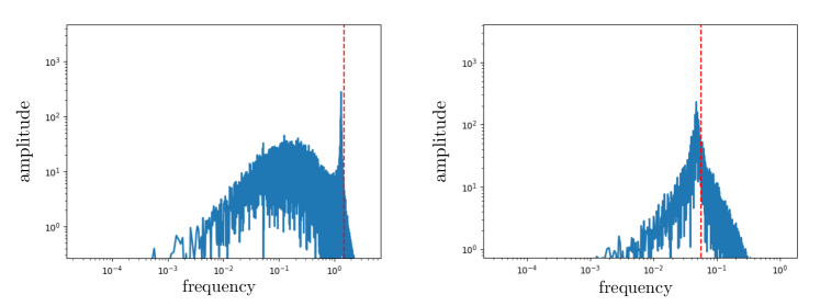
The thermostat should be in resonance with the system’s fluctuations [9]. In Fig. (7) a spectral analysis is shown of the time series of for and with a relativistic temperature and . The red line is the thermostat mode calculated from Eq. (28). There, the spectrum has a clear peak. The other frequencies come from the particle system. For small values of the peak is sharper and the thermostat is separated from the system. The thermostat mode should mix with the system’s modes and therefore a situation at the left of fig. 7 is desirable. In that case (), canonical energy fluctuations are observed as can be seen in fig. 6.
IV Conclusion
Summarizing, the numerical experiments in three dimensions confirmed that the Jüttner distribution is a very good generalisation of the Maxwell-Boltzmann distribution to special relativity. The results are independent of the particle masses.
The temperature was determined from the momenta of the particles using the equipartition theorem. From the fact that we employed periodic boundary conditions arises the uniqueness of this definition: We have a special frame of reference (the boundaries) and the temperature is determined from the momenta as measured in this frame.
Despite of the Jüttner function not being Lorentz invariant, it gives the correct distribution in this frame of reference. To investigate this further, one could generate histograms with constant rapidity bins as proposed in Ref. [5] and compare them to a three dimensional generalisation of the Lorentz invariant distribution function that was derived in their paper.
The interaction between particles was assumed to happen instantaneously which is theoretically not consistent with special relativity. In order to overcome this problem one could introduce fields and calculate the force from a retarded potential. However, since the potential is short-ranged it can be assumed that this effect will not result in a different velocity distribution. Whether this has an effect on other quantities beside the velocity distribution, e.g. the heat capacity, could be investigated in further simulations.
A Nosé-Poincaré thermostat was coupled to a relativistic particle system. This allowed to control the temperature simulating the canonical ensemble. The appropriate range for the thermal inertia could be determined by monitoring the kinetic energy fluctuations. The behaviour of those fluctuations is similar to that of a thermostatted classical system [12] and in that regime they should fulfill the fluctuation - dissipation theorem. The thermostat itself exhibits a frequency that is visible in the spectrum of (which represents the friction parameter in the equations of motion). If is in the appropriate range, the thermostat mode mixes with the frequencies of the particle system and thus the thermostat couples to the particles and canonical energy fluctuations are obtained.
References
- Jüttner [1911] F. Jüttner, Das Maxwellsche Gesetz der Geschwindigkeitsverteilung in der Relativtheorie, Annalen der Physik 339, 856 (1911).
- Cubero et al. [2007] D. Cubero, J. Casado-Pascual, J. Dunkel, P. Talkner, and P. Hänggi, Thermal equilibrium and statistical thermometers in special relativity, Physical Review Letters 99, 10.1103/physrevlett.99.170601 (2007).
- Dunkel et al. [2007] J. Dunkel, P. Talkner, and P. Hänggi, Relative entropy, haar measures and relativistic canonical velocity distributions, New Journal of Physics 9, 144 (2007).
- Ghodrat and Montakhab [2011] M. Ghodrat and A. Montakhab, Molecular dynamics simulation of a relativistic gas: Thermostatistical properties, Computer Physics Communications 182, 1909 (2011).
- Curado et al. [2016] E. M. Curado, F. T. Germani, and I. D. Soares, Search for a Lorentz invariant velocity distribution of a relativistic gas, Physica A: Statistical Mechanics and its Applications 444, 963 (2016).
- Chacón-Acosta et al. [2010] G. Chacón-Acosta, L. Dagdug, and H. Morales-Tecotl, On the manifestly covariant Juttner distribution and equipartition theorem, Physical review. E, Statistical, nonlinear, and soft matter physics 81, 021126 (2010).
- Mendoza et al. [2012] M. Mendoza, N. A. M. Araújo, S. Succi, and H. J. Herrmann, Transition in the equilibrium distribution function of relativistic particles, Scientific Reports 2, 611 (2012).
- Allen and Tildesley [1990] M. P. Allen and D. J. Tildesley, Computer Simulation of Liquids (Clarendon Press, Oxford, 1990).
- Shuichi [1991] N. Shuichi, Constant Temperature Molecular Dynamics Methods, Progress of Theoretical Physics Supplement 103, 1 (1991), https://academic.oup.com/ptps/article-pdf/doi/10.1143/PTPS.103.1/5351100/103-1.pdf .
- Bond et al. [1999] S. D. Bond, B. J. Leimkuhler, and B. B. Laird, The Nosé–Poincaré method for constant temperature molecular dynamics, Journal of Computational Physics 151, 114 (1999).
- Nosé [1984] S. Nosé, A molecular dynamics method for simulations in the canonical ensemble, Molecular Physics 52, 255 (1984), https://doi.org/10.1080/00268978400101201 .
- Valenzuela et al. [2014] G. Valenzuela, J. Saavedra, R. E. Rozas, and P. Toledo, Analysis of energy and friction coefficient fluctuations of a Lennard-Jones liquid coupled to the Nosé–Hoover thermostat, Molecular Simulation 41, 1 (2014).