Extending solid-state calculations to ultra long-range length scales

Abstract

We present a method which enables solid-state density functional theory calculations to be applied to systems of almost unlimited size. Computations of physical effects up to the micron length scale but which nevertheless depend on the microscopic details of the electronic structure, are made possible. Our approach is based on a generalization of the Bloch state which involves an additional sum over a finer grid in reciprocal space around each ${\bf k}$-point. We show that this allows for modulations in the density and magnetization of arbitrary length on top of a lattice-periodic solution. Based on this, we derive a set of ultra long-range Kohn-Sham equations. We demonstrate our method with a sample calculation of bulk LiF subjected to an arbitrary external potential containing nearly 3500 atoms. We also confirm the accuracy of the method by comparing the spin density wave state of bcc Cr against a direct super-cell calculation starting from a random magnetization density. Furthermore, the spin spiral state of $\gamma$-Fe is correctly reproduced and the screening by the density of a saw-tooth potential over 20 unit cells of silicon is verified.

I Introduction

Density functional theory (DFT) Hohenberg and Kohn (1964) has had a tremendous impact on solid-state physics and is, due to its computational efficiency, at the heart of modern computer based material research. Since its original proposal, further developing DFT has been an ongoing process. Extensions to DFT typically include extra densities in addition to the charge density, such as the magnetization von Barth and Hedin (1972), current density Vignale and Rasolt (1987) or the superconducting order-parameter Oliveira et al. (1988). Another fundamental extension of DFT was the generalization to time-dependent systems Runge and Gross (1984) enabling accurate calculations of dynamical properties of molecules and solids. While these extensions allowed for a more in-depth understanding of microscopic properties, not much progress has been made in applying DFT to effects in solids occurring on larger, mesoscopic length scales. Such effects include long-ranged quasiparticles, magnetic domains or spatially dependent electric fields. As DFT is a formally exact theory, the underlying physics for such phenomena are readily at hand, yet actual calculations remain very difficult. In a typical calculation, a single unit cell is solved with periodic boundary conditions, thus effects extending far beyond the size of a single unit cell are lost. While it is, in principle, possible to use ever larger super-cells, in practice one quickly reaches the limit of computational viability. This is mostly due to the poor scaling with the number of atoms, $\sim\mathcal{O}(N_{\rm atom}^{3})$, which plagues all computer programs with a systematic basis set and limits calculations to systems containing a maximum of $\sim 1000$ atoms. Recent progress based on linear scaling approaches Goedecker (1999) was able to increase the computable system size considerably. Linear scaling approaches, however, require a “nearsightedness” of the system. While this might be fulfilled for effects strictly related to the charge density, this is certainly not fulfilled for large magnetic systems, such as magnetic domains.

In this work we propose a fundamentally different approach to drastically extend the length scale of DFT calculations without significantly increasing the computational cost. Our approach relies on altered Bloch states and can be understood as a generalization of the spin-spiral ansatzSandratskii (1986), which emerges as a special case of our ansatz. In the spin-spiral ansatz, a momentum-dependent phase is added to the normal Bloch state. It then becomes possible to compute a large, extended spiraling magnetic moment with a single unit cell. While this is computationally very efficient, it is, at the same time, the biggest limitation of the spin-spiral ansatz: It allows only for a change in the direction of the magnetization while the magnitude of the magnetization and the charge density remain unaltered. We overcome this limitation by introducing an additional sum in the Bloch states over a finer grid in reciprocal space around each ${\bf k}$-point. The resulting densities then become a Fourier series with a controllable periodicity, which may extend far beyond the length scale of a single unit cell.

II Ultra long-range ansatz

The systems we will focus on in this article are described by the Kohn-Sham (KS) Hamiltonian of spin-density functional theory (atomic units are used throughout):

$$\hat{H}_{0}=-\frac{\nabla^{2}}{2}+v_{s}({\bf r})+{\bf B}_{s}({\bf r})\cdot\bm{\sigma}.$$ (1)

The KS potential $v_{s}({\bf r})=v_{\rm ext}({\bf r})+v_{\rm H}({\bf r})+v_{\rm xc}({\bf r})$ consists of an external potential $v_{\rm ext}$, a Hartree potential $v_{\rm H}$ and an exchange-correlation (xc) potential $v_{\rm xc}$. Similarly, the KS magnetic field ${\bf B}_{s}({\bf r})=\frac{1}{2c}{\bf B}_{\rm ext}({\bf r})+{\bf B}_{\rm xc}({\bf r})$ can be decomposed into an external field ${\bf B}_{\rm ext}$ and an xc-field ${\bf B}_{\rm xc}$.

We will start off by extending the KS wave functions. From that we will derive altered charge and magnetization densities. Finally we will derive a long-range Hamiltonian and the matrix elements associated with it.

II.1 Wave function and densities

Bloch states of the form $\varphi_{i{\bf k}}({\bf r})=u_{i{\bf k}}({\bf r})e^{i{\bf k}\cdot{\bf r}}$, where $u_{i{\bf k}}$ is a lattice-periodic spinor function, are used in standard solid-state calculations. The central idea of our approach is a generalization of this Bloch state to include long-range fluctuations. A similar idea was put forward with the spin-spiral ansatzSandratskii (1986), where a momentum-dependent phase is applied to the normal Bloch spinor state. Our ultra long-range ansatz employs, in addition, momentum-dependent expansion coefficients which allow for changes in magnitude of the densities from cell to cell. For a fixed ${\bf k}$-vector our new Bloch-like state reads:

$$\Phi_{\alpha}^{{\bf k}}({\bf r}) =\frac{1}{\sqrt{N_{u}}}\sum_{i\bm{\kappa}}c^{\alpha}_{i{\bf k}+\bm{\kappa}}\begin{pmatrix}u_{i{\bf k}}^{\uparrow}({\bf r})\\ u_{i{\bf k}}^{\downarrow}({\bf r})\end{pmatrix}e^{i({\bf k}+\bm{\kappa})\cdot{\bf r}}$$ (2)

where $u_{i{\bf k}}^{\uparrow\downarrow}$ are the normalized orbitals of a lattice-periodic system, $i$ is a band index and ${\bf k}$ a reciprocal space vector, $c^{\alpha}_{i{\bf k}+\bm{\kappa}}$ are complex coefficients to be determined variationally (or by propagating in time) and $\alpha$ labels a particular long-range state. The vectors $\bm{\kappa}$ live on a finer grid around each ${\bf k}$-point in reciprocal space (Fig. 1(a)), which we use to sample long-range effects. Finally $N_{u}$ is a normalization factor which is equal to the number of unit cells on which $\Phi_{\alpha}^{{\bf k}}$ is periodic. Note that we have used the lattice periodic parts of the orbitals at ${\bf k}$ and not ${\bf k}+\bm{\kappa}$. In principle, both are complete basis sets capable of expanding any lattice-periodic function. In practice, the choice of using $u_{i{\bf k}}^{\uparrow\downarrow}$ over $u^{\uparrow\downarrow}_{i{\bf k}+\bm{\kappa}}$ is more efficient for determining the density, magnetization and Hamiltonian matrix elements.

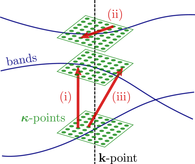
(a)

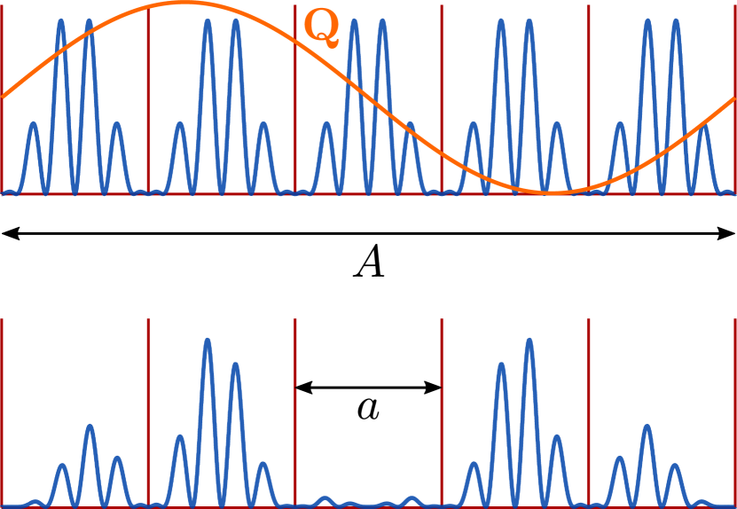
(b)

Figure 1: (a) Schematic of the $\bm{\kappa}$-point grid. For each ${\bf k}$-point (black dashed line) all bands (blue) are augmented with a fine grid of $\bm{\kappa}$-points (green). Three different types of couplings between $\bm{\kappa}$-points corresponding to different length scales are possible. (i) A coupling between two identical $\bm{\kappa}$-points but with different band indices (ii) a coupling between different $\bm{\kappa}$-points sharing the same band index, and (iii) a coupling between different $\bm{\kappa}$-points with different band indices. The maximum length scale of the calculation may be chosen by adjusting the $\bm{\kappa}$-point grid. (b) A schematic of the long range approach. The red lines indicate unit cells. The lattice periodic density $\rho_{{\bf Q}}$ (blue) is altered by a ${\bf Q}$-dependent modulation (orange) with a different periodicity. The result (lower graph) depends on both, the long-range modulation and the lattice periodic solution. $a$ is the lattice constant of a unit cell and $A$ is the lattice constant of the ultracell, which is the smallest cell that contains the full long-range solution.

From this wave function, we can construct a charge and magnetization density:

$$\rho({\bf r})=\frac{1}{N_{k}}\sum_{{\bf k},\alpha}f_{\alpha}^{{\bf k}}\Phi_{\alpha}^{{\bf k}\dagger}({\bf r})\Phi_{\alpha}^{{\bf k}}({\bf r})$$ (3)

$${\bf m}({\bf r})=\frac{1}{N_{k}}\sum_{{\bf k},\alpha}f_{\alpha}^{{\bf k}}\Phi_{\alpha}^{{\bf k}\dagger}({\bf r})\bm{\sigma}\Phi_{\alpha}^{{\bf k}}({\bf r})$$ (4)

with the number of ${\bf k}$-points $N_{{\bf k}}$ and the ultra long-range occupation numbers $f_{\alpha}^{{\bf k}}$ associated with the orbitals $\Phi_{\alpha}^{{\bf k}}$. The charge and magnetization density obtained from this wave function take the form

$$\begin{split}\rho({\bf r})&=\sum_{{\bf Q}}\rho_{{\bf Q}}({\bf r})e^{i{\bf Q}\cdot{\bf r}},\\ {\bf m}({\bf r})&=\sum_{\bf Q}{\bf m}_{\bf Q}({\bf r})e^{i{\bf Q}\cdot{\bf r}}\end{split}$$ (5)

with ${\bf Q}=\bm{\kappa}-\bm{\kappa^{\prime}}$. The partial densities $\rho_{{\bf Q}}$ and ${\bf m}_{{\bf Q}}$ in Eq. (5) are complex in general and act as lattice-periodic Fourier coefficients. The resulting real-space densities $\rho({\bf r})$ and ${\bf m}({\bf r})$ are real functions, which, depending on the values of ${\bf Q}$, will have a periodicity larger than the length scale of a unit cell (Fig. 1(b)). By adjusting the underlying $\bm{\kappa}$-lattice, it is therefore possible to change the ${\bf Q}$-vectors and hence allow for variations of arbitrary length in the system. The ${\bf Q}=0$ term deserves special mention, as it corresponds to the full lattice-periodic solution. We emphasize that there is no restriction on the magnitude of $\rho_{{\bf Q}},{\bf m}_{{\bf Q}}$ and we are thus able to expand arbitrary modulations in the charge and magnetization densities. This is a key difference compared to the spin-spiral ansatz Sandratskii (1986).

The Fourier coefficients $\rho_{{\bf Q}}$ and ${\bf m}_{{\bf Q}}$ can be calculated efficiently by first calculating the wave function in Eq. (2) for a subset of unit cells given by a set of real-space lattice vectors $\{{\bf R}_{i}\}$. We choose the ${\bf R}_{i}$-vectors to be the conjugate real-space vectors of the ${\bf Q}$-vectors. The wave function in a single unit cell is then given by a sum over $n$ and a fast Fourier transform in $\bm{\kappa}$ of the coefficients $c^{\alpha}_{n{\bf k}+\bm{\kappa}}$:

$$\Phi_{\alpha}^{{\bf k}}({\bf r}+{\bf R}_{i})\approx e^{i{\bf k}\cdot({\bf r}+{\bf R}_{i})}\sum_{n}\begin{pmatrix}u_{n{\bf k}}^{\uparrow}({\bf r})\\ u_{n{\bf k}}^{\downarrow}({\bf r})\end{pmatrix}\sum_{\bm{\kappa}}c^{\alpha}_{n{\bf k}+\bm{\kappa}}e^{i\bm{\kappa}\cdot{\bf R}_{i}}$$ (6)

where ${\bf r}$ is restricted to a single unit cell and we have assumed that $|\bm{\kappa}\cdot{\bf r}|\ll 1$. Note also that the normalization constant $1/\sqrt{N_{u}}$ has been removed. This ensures that observables such as charge and energy are calculated per unit cell rather than per ultracell. From this, we compute the charge and magnetization densities on the same grid, i.e. $\rho_{i}=\rho({\bf r}+{\bf R}_{i})$ and ${\bf m}_{i}={\bf m}({\bf r}+{\bf R}_{i})$. This set can then be partially (fast) Fourier transformed to reciprocal space to obtain $\rho_{{\bf Q}}({\bf r})$ and ${\bf m}_{{\bf Q}}({\bf r})$:

$$\begin{split}\rho_{\bf Q}({\bf r})&=\frac{1}{N_{{\bf R}}}\sum_{i}\rho({\bf r}+{\bf R}_{i})\,e^{-i{\bf Q}\cdot{\bf R}_{i}}\\ {\bf m}_{\bf Q}({\bf r})&=\frac{1}{N_{{\bf R}}}\sum_{i}{\bf m}({\bf r}+{\bf R}_{i})\,e^{-i{\bf Q}\cdot{\bf R}_{i}}\end{split}$$ (7)

Here $N_{{\bf R}}$ denotes the number of ${\bf R}$-vectors chosen. With the densities at hand, we will now focus on generalizing the Hamiltonian such that meaningful, non-trivial values for the expansion coefficients $c^{\alpha}_{n{\bf k}+\bm{\kappa}}$ in Eq. (2) are obtained.

II.2 Long-range Hamiltonian

The ultra long-range Hamiltonian retains the full lattice periodic KS Hamiltonian $\hat{H}_{0}$ given in Eq. (1), but also has an additional “modulation” term

$$\hat{H}=\hat{H}_{0}+\sum_{{\bf Q}}\hat{H}_{{\bf Q}}({\bf r})e^{i{\bf Q}\cdot{\bf r}}.$$ (8)

The total Hamiltonian $\hat{H}$ is thus decomposed in the same way as the charge and magnetization densities in Eq. (5). For a KS system like Eq. (1), our “modulation” Hamiltonian reads

$$\hat{H}_{{\bf Q}}\left({\bf r}\right)=V_{{\bf Q}}({\bf r})+{\bf B}_{{\bf Q}}({\bf r})\cdot\bm{\sigma},$$ (9)

where $V_{{\bf Q}}({\bf r})$ and ${\bf B}_{{\bf Q}}({\bf r})$ are again complex, lattice periodic Fourier coefficients and contribute to long-ranged versions of the scalar potential and the magnetic field, respectively. In the following we will discuss these coefficients and how to compute them in more detail. We will start with the scalar potential, which can again be decomposed into an external potential $V_{{\bf Q}}^{\rm ext}({\bf r})$, a Hartree potential $V^{\rm H}_{{\bf Q}}({\bf r})$ and an xc-potential $V^{\rm xc}_{{\bf Q}}({\bf r})$. The coefficients $V_{{\bf Q}}^{\rm ext}({\bf r})$ of an external, long-ranged potential can be freely chosen. The coefficients for the long-ranged Hartree potential $V^{\rm H}_{{\bf Q}}({\bf r})$ are obtained from the long-range density in Eq. (5):

$$V^{\rm H}_{{\bf Q}}({\bf r})=\int d^{3}r^{\prime}\frac{\rho_{{\bf Q}}({\bf r^{\prime}})}{\left|{\bf r}-{\bf r^{\prime}}\right|}e^{-i{\bf Q}\cdot({\bf r}-{\bf r}^{\prime})}.$$ (10)

This may be performed efficiently by further Fourier transforming $\rho_{{\bf Q}}({\bf r})$ to $\rho_{{\bf Q}}({\bf G})$ where ${\bf G}$ is a reciprocal lattice vector. The Hartree potential is then determined directly via $V^{\rm H}_{{\bf Q}}({\bf G})=4\pi\rho_{{\bf Q}}({\bf G})/|{\bf G}+{\bf Q}|^{2}$ and can be subsequently Fourier transformed back to real-space. This is easily extended to the case of the augmented plane wave basis by using the method of Weinert Weinert (1981).

Next we will determine the coefficients associated with the xc-interaction. An important difference compared to the Hartree potential is that the xc-functional is inherently non-linear, therefore the naive approach $V_{{\bf Q}}^{\rm xc}=V_{\rm xc}[\rho_{{\bf Q}}]$ may introduce a mixing of the real and imaginary part of $\rho_{{\bf Q}}$. Instead we first Fourier transform the density to real-space, $\rho_{{\bf R}_{i}}({\bf r})$, and then evaluate the xc-potential separately for each ${\bf R}$-vector. The inverse Fourier transform is then applied to obtain

$$V_{{\bf Q}}^{\rm xc}({\bf r})=\frac{1}{N_{{\bf R}}}\sum_{i}V_{\rm xc}\left[\rho_{{\bf R}_{i}}\right]({\bf r})e^{-i{\bf Q}\cdot{\bf R}_{i}}.$$ (11)

It is worth noting that defining the long-range xc-functional this way does not change how local an xc-functional inherently is, it is merely a Fourier interpolation.

The magnetic field ${\bf B}_{{\bf Q}}$ in Eq. (9) consists of an external field, an xc-field and a dipole-dipole field:

$${\bf B}_{{\bf Q}}({\bf r})=\frac{1}{2c}{\bf B}_{{\bf Q}}^{\rm ext}({\bf r})+{\bf B}_{{\bf Q}}^{\rm xc}({\bf r})+\frac{1}{2c}{\bf B}_{{\bf Q}}^{\rm D}({\bf r}).$$ (12)

Again, the external magnetic field may be chosen arbitrarily and the xc-field can be computed analogously to the xc-potential

$${\bf B}_{{\bf Q}}^{\rm xc}\left({\bf r}\right)=\frac{1}{N_{{\bf R}}}\sum_{i}{\bf B}_{\rm xc}\left[\rho_{{\bf R}_{i}},{\bf m}_{{\bf R}_{i}}\right]({\bf r})e^{-i{\bf Q}\cdot{\bf R}_{i}}.$$ (13)

The last term in Eq. (12) corresponds to the magnetic field associated with the magnetostatic dipole-dipole interaction

$${\bf B}_{{\bf Q}}^{\rm D}\left({\bf r}\right)=\frac{1}{2c}\int d^{3}r^{\prime}\,\frac{3\,{\bf e}_{{\bf r}-{\bf r^{\prime}}}\left({\bf m}_{{\bf Q}}({\bf r^{\prime}})\cdot{\bf e}_{{\bf r}-{\bf r^{\prime}}}\right)-{\bf m}_{{\bf Q}}({\bf r^{\prime}})}{\left|{\bf r}-{\bf r}^{\prime}\right|^{3}}e^{-i{\bf Q}\cdot({\bf r}-{\bf r}^{\prime})},$$ (14)

where ${\bf e}_{{\bf r}-{\bf r^{\prime}}}$ is the unit vector along the direction ${\bf r}-{\bf r^{\prime}}$. The contribution of the dipole-dipole interaction is typically neglected in DFT calculations as it is usually small in comparison with ${\bf B}^{\rm xc}$, which originates from the Coulomb exchange interaction. As the coulomb exchange interaction is inherently short ranged, the magnetic dipole-dipole interaction is expected to have a significant contribution at larger length scales. We therefore include this term in the “modulation” Hamiltonian. The derivation of a truly non-local, ${\bf Q}$-dependent xc-potential is beyond the scope of this article but has been addressed by Pellegrini, et. alPellegrini et al. (2020) for the dipole interaction.

We conclude this section with a remark on the kinetic energy. The kinetic energy operator ${\bf\hat{p}}^{2}/2$ does not explicitly depend on the periodicity of the problem at hand. As the kinetic energy operator is already included in $\hat{H}_{0}$ (Eqs. (1), (8)), it should not be added to $\hat{H}_{{\bf Q}}$. It is important to note, however, that the kinetic energy is sensitive to the shifts in reciprocal space of the wave function (Eq. (2)) ${\bf k}\rightarrow{\bf k}+\bm{\kappa}$ which should be taken into account.

II.3 Hamiltonian Matrix Elements

We will now focus on diagonalizing the long-range Hamiltonian in Eq. (8). For that we compute the matrix elements for a fixed ${\bf k}$-point in the orbital basis of Eq. (2) to evaluate

$$\left\langle\varphi_{i{\bf k}+\bm{\kappa}}\right|\hat{H}_{0}+\hat{H}_{{\bf Q}}\left|\varphi_{j{\bf k}+\bm{\kappa^{\prime}}}\right\rangle=\delta_{\bm{\kappa},\bm{\kappa^{\prime}}}\left(O_{{\bf k}+\bm{\kappa},{\bf k}}^{{\dagger}}\epsilon_{{\bf k}+\bm{\kappa}}^{0}O_{{\bf k}+\bm{\kappa},{\bf k}}\right)_{ij}+\left\langle\varphi_{i{\bf k}+\bm{\kappa}}\right|\hat{H}_{{\bf Q}}\left|\varphi_{j{\bf k}+\bm{\kappa^{\prime}}}\right\rangle.$$ (15)

Here ${\bf Q}=\bm{\kappa}-\bm{\kappa^{\prime}}$, $\epsilon_{{\bf k}+\bm{\kappa}}^{0}$ is the diagonal matrix of eigenvalues of $\hat{H}_{0}$ at ${\bf k}+\bm{\kappa}$ and $O_{{\bf k}+\bm{\kappa},{\bf k}}$ is the unitary overlap matrix between the orbitals at ${\bf k}$ and ${\bf k}+\bm{\kappa}$, i.e.

$$\left(O_{{\bf k}+\bm{\kappa},{\bf k}}\right)_{ij}=\sum_{s}\int d^{3}r\,\varphi_{is{\bf k}+\bm{\kappa}}^{*}({\bf r})\exp(i\bm{\kappa}\cdot{\bf r})\varphi_{js{\bf k}}({\bf r}).$$ (16)

This overlap matrix is required because our chosen basis is the set of orbitals at ${\bf k}$ and not those at ${\bf k}+\bm{\kappa}$. The overlap matrix $O_{{\bf k}+\bm{\kappa},{\bf k}}$ may however not be strictly unitary in practice. This may be because of numerical inaccuracies but also because the basis is finite and there could be bands of a particular character at some $({\bf k}+\bm{\kappa})$-points but not at others. Unitarity is necessary for preserving the eigenvalues $\epsilon_{{\bf k}+\bm{\kappa}}^{0}$ and we ensure this by first performing a singular value decomposition $O_{{\bf k}+\bm{\kappa},{\bf k}}=U\Sigma T^{{\dagger}}$ and then making the substitution $O_{{\bf k}+\bm{\kappa},{\bf k}}\rightarrow UT^{{\dagger}}$. One can show that this new matrix is the closest (in the sense of the Frobenius norm) unitary matrix to the original.

What remains to be done is the calculation of the matrix elements of $\hat{H}_{{\bf Q}}$ in Eq. (9). We start with the the scalar potential and find:

$$\left\langle\varphi_{n{\bf k}}^{\bm{\kappa}}\right|\hat{V}_{{\bf Q}}\left|\varphi_{n^{\prime}{\bf k}}^{\bm{\kappa^{\prime}}}\right\rangle=\sum_{s}\int_{\rm unit}d^{3}r\,u_{ns{\bf k}}^{*}({\bf r})u_{n^{\prime}s{\bf k}}({\bf r})V_{{\bf Q}}\left({\bf r}\right),$$ (17)

where $s=\uparrow,\downarrow$ is a spin index. Here we have defined $\varphi_{n{\bf k}}^{\bm{\kappa}}({\bf r})\equiv\varphi_{n{\bf k}}({\bf r})e^{i\bm{\kappa}\cdot{\bf r}}$. In the first step we converted the integral over the ultracell into an integral over a unit cell and a sum over all unit cells in the ultracell $\int_{\rm ultra}d^{3}r\to\sum_{{\bf R}_{u}}\int_{\rm unit}d^{3}r$ and made use of the lattice periodicity of $u_{n{\bf k}}({\bf r})$. In the second step we then carried out the sum over ${\bf R}_{u}$ followed by the sum over ${\bf Q}$. The matrix elements for the ultracell can thus be expressed by a simple unit cell integration. Similarly we find for the magnetic field contribution:

$$\begin{split}\left\langle\varphi_{n{\bf k}}^{\bm{\kappa}}\right|\hat{\bf B}_{\bf Q}\cdot\bm{\sigma}\left|\varphi_{n^{\prime}{\bf k}}^{\bm{\kappa^{\prime}}}\right\rangle=\int_{\rm unit}d^{3}r\,&u_{\uparrow n{\bf k}}^{*}({\bf r})u_{\downarrow n^{\prime}{\bf k}}({\bf r})\left(B_{\bf Q}^{x}({\bf r})-iB_{\bf Q}^{y}({\bf r})\right)\\ +&u_{\downarrow n{\bf k}}^{*}({\bf r})u_{\uparrow n^{\prime}{\bf k}}({\bf r})\left(B_{\bf Q}^{x}({\bf r})+iB_{\bf Q}^{y}({\bf r})\right)\\ +&\left(u_{\uparrow n{\bf k}}^{*}({\bf r})u_{\uparrow n^{\prime}{\bf k}}({\bf r})-u_{\downarrow n{\bf k}}^{*}({\bf r})u_{\downarrow n^{\prime}{\bf k}}({\bf r})\right)B_{\bf Q}^{z}({\bf r}).\end{split}$$ (18)

III Numerical implementation

In this section we will address how to implement the ultra long-range ansatz in practice. The discussions in this section are based on our implementation in the Elk electronic structure code elk , which is an all-electron code using the full potential linearized augmented plane wave (FP-LAPW) method.

III.1 Self-consistent solution

$\hat{H}$ in Eq. (8) is a KS system in which the potentials are functionals of the partial densities $\rho_{\bf Q}({\bf r})$ and ${\bf m}_{\bf Q}({\bf r})$ in Eq. (7), which in turn depend on the orbitals $\Phi_{\alpha}^{\bf k}({\bf r})$ from Eq. (2). Equation (8) thus needs to be solved self-consistently. We employ an iteration scheme as it is usually done when solving KS systems:

1. Solve the lattice periodic ground state, Eq. (1) and obtain the spinor orbitals $\begin{pmatrix}u_{n{\bf k}}^{\uparrow}({\bf r})\\ u_{n{\bf k}}^{\downarrow}({\bf r})\end{pmatrix}$ as well as all Eigen energies $\epsilon^{0}_{n{\bf k}+\bm{\kappa}}$ associated with the ${\bf k}+\bm{\kappa}$-points. 2. Initialize the external long-range potentials via $V_{\bf Q}$ and ${\bf B}_{\bf Q}$ and the occupation numbers $f^{\bf k}_{\alpha}$. 3. (a) Compute the matrix elements of $\hat{H}_{\bf Q}$ in Eq. (9). Diagonalize $\hat{H}$ in Eq. (8) to obtain the expansion coefficients $c^{\alpha}_{n{\bf k}+\bm{\kappa}}$ as well as the long-range Eigen-energies $\epsilon^{\bf k}_{\alpha}$ for each ${\bf k}$-point. (b) Concurrently with the step above, accumulate the long-range densities $\rho_{\bf Q}({\bf r})$ and ${\bf m}_{\bf Q}({\bf r})$ from Eqs. (3) and (4). This is performed most efficiently by first calculating the long-range orbitals explicitly in real-space: $\Phi_{\alpha}^{{\bf k}}({\bf r}+{\bf R}_{i})$. 4. Calculate the new occupation numbers $f^{\bf k}_{\alpha}$. 5. Calculate new long-range potentials $V_{\bf Q}^{\prime}$ and ${\bf B}_{\bf Q}^{\prime}$. Mix the new potentials with the potentials from the previous iteration. Monitor the relative change in the potentials. 6. Repeat steps 3 to 5 until the change in the potentials is sufficiently small.

We will discuss two steps in this self-consistent cycle in more detail.

First we will explain the order of calculating the energies $\epsilon^{\bf k}_{\alpha}$ first, the densities $\rho_{\bf Q}({\bf r})$ and ${\bf m}_{\bf Q}({\bf r})$ second and the occupation numbers $f_{\alpha}^{\bf k}$ third. This seems counter-intuitive, as the densities depend on the occupation numbers (Eqs. (3) and (4)). However, as we are performing a self-consistent cycle, the occupation numbers will converge to the correct value as self-consistency is achieved. Computing the occupation numbers last enables us to parallelize step 3 over the ${\bf k}$-point set in a single loop: For each ${\bf k}$-point, we diagonalize $\hat{H}^{\bf k}=\hat{H}^{\bf k}_{0}+\hat{H}^{\bf k}_{\bf Q}$ and simultaneously compute $\rho^{\bf k}_{\bf Q}({\bf r})$ and ${\bf m}^{\bf k}_{\bf Q}({\bf r})$. These are added to the total density and magnetization. The central computational gain is that this ordering is much less demanding when it comes to memory: the coefficients $c^{\alpha}_{n{\bf k}+\bm{\kappa}}$ do not have to be stored but can be calculated and used on-the-fly instead.

Second, we note that some care has to be taken during the mixing. We choose to mix the complex Fourier coefficients $V_{\bf Q}({\bf r})$ and ${\bf B}_{\bf Q}({\bf r})$ rather than their real-space counterparts. We also want to emphasize that in a typical calculation a rather slow mixing should be applied. The Coulomb interaction in a large system will react very strongly to any external perturbation because of the divergence of $1/Q^{2}$. This can lead to substantial charge sloshing during convergence necessitating the use of a small mixing parameter. This is an aspect of the method which would benefit from further investigation and improvement. One possibility is to use a screened Coulomb interaction to remove the divergence. This screening could be slowly reduced to zero during the self-consistent loop to improve the rate of convergence.

III.2 ${\bf k}$-point grids

The underlying grids have to be chosen carefully in order to avoid computational artifacts and to achieve a most efficient calculation. Ideally, the smallest distance between ${\bf k}$-points should be greater than the largest distance between $\bm{\kappa}$-points, i.e. $\left|\bm{\kappa}-\bm{\kappa^{\prime}}\right|<\left|{\bf k}-{\bf k^{\prime}}\right|$. This will ensure that the set ${\bf k}+\bm{\kappa}$ does not overlap for any two ${\bf k}$-points, which may lead to double counting and an over-complete basis set. Physically speaking, the length scales in the system should be well separated, i.e. the modulation should be far larger than the size of a unit cell. If $\left|\bm{\kappa}-\bm{\kappa^{\prime}}\right|\approx\left|{\bf k}-{\bf k}^{\prime}\right|$, however, the system tends to have a size which can and should be solved with a super-cell instead.

Many Fourier transformations need to be carried out during each self-consistent step: with $e^{-i\bm{\kappa}\cdot{\bf R}_{i}}$ when calculating the wave function in Eq. (6), and with $e^{-i{\bf Q}\cdot{\bf R}}$ when calculating the densities in Eqs. (3) and (4); and the xc-potential and -field, Eqs. (11) and (13). This constitutes a major part of the computational effort and it is therefore highly beneficial to carry out all Fourier transformations via a Fast Fourier Transform (FFT). This requires the underlying grid to be FFT compatible (having, in our case, radices 2, 3, 5 and 7). Owing to ${\bf Q}=\bm{\kappa}-\bm{\kappa^{\prime}}$ the ${\bf Q}$-point and the $\bm{\kappa}$-point grids are dependent on one another. The number of ${\bf Q}$-points $n_{\bf Q}$ along a given direction $i$ is $n_{\bf Q}^{i}=2n_{\bm{\kappa}}^{i}-1$. In our implementation, we ensure that the input ${\bf Q}$-grid snaps to the next FFT compatible grid. We then choose the $\bm{\kappa}$-point grid such that $2n_{\bm{\kappa}}^{i}-1\leq n^{i}_{\bf Q}$. This grid choice can sometimes result in unmatched ${\bf Q}$-points, e.g. if $n_{\bf Q}=20$ and $n_{\bm{\kappa}}=10$ then the ${\bf Q}$-vectors are not symmetric around zero. While the unmatched ${\bf Q}$-point is “dead-weight” and remains zero throughout the calculation, the speed up obtained by using a FFT outweighs having additional ${\bf Q}$-points.

III.3 Computation of the Hartree and dipole interaction

We will briefly address how to calculate the complex integrals appearing in the scalar potential, Eq. (10), and the magnetic field, Eq. (14). When computing the Hartree-potential in Eq. (10), we solve Poisson’s equation using the method by WeinertWeinert (1981), which can be generalized to complex densities relatively easily.

The dipole interaction, Eq. (14), can be solved for in a similar way by evaluating Poisson’s equation component-wise for the vector potential. From classical electrodynamics, the vector potential associated with a magnetization is given by:

$${\bf A}^{\rm dip}({\bf r})=\frac{1}{c}\int d^{3}r^{\prime}\frac{\nabla\times{\bf m}\left({\bf r^{\prime}}\right)}{\left|{\bf r}-{\bf r^{\prime}}\right|}$$ (19)

We partially Fourier transform both sides and obtain:

$$\sum_{\bf Q}{\bf A}^{\rm dip}_{\bf Q}\left({\bf r}\right)e^{i{\bf Q}\cdot{\bf r}}=\frac{1}{c}\int d^{3}r^{\prime}\,\frac{\nabla\times\sum_{\bf Q}{\bf m}_{\bf Q}({\bf r^{\prime}})e^{i{\bf Q}\cdot{\bf r}^{\prime}}}{\left|{\bf r}-{\bf r}^{\prime}\right|}.$$ (20)

We thus obtain for the coefficients of the vector potential:

$$A_{{\bf Q},j}^{\rm dip}({\bf r})=\frac{1}{c}\sum_{kl}\epsilon_{jkl}\int d^{3}r^{\prime}\,e^{-i{\bf Q}\cdot\left({\bf r}-{\bf r}^{\prime}\right)}\frac{\partial_{k}m_{{\bf Q},l}({\bf r}^{\prime})+iQ_{k}m_{{\bf Q},l}({\bf r}^{\prime})}{\left|{\bf r}-{\bf r}^{\prime}\right|}$$ (21)

Here $j,k,l$ indicate vector components and $\epsilon_{jkl}$ is the Levi-Civita symbol. The coefficients ${\bf A}_{\bf Q}^{\rm dip}({\bf r})$ now have the same form as the Hartree potential, Eq. (10), and can also be computed by a complex version of Weinert’s method Weinert (1981). From this it is easy to obtain the magnetic field of the dipole interaction via ${\bf B}^{\rm dip}({\bf r})=\nabla\times{\bf A}^{\rm dip}({\bf r})$. We find for the coefficients:

$$B_{{\bf Q},j}^{\rm dip}=\sum_{kl}\epsilon_{jkl}\left[\partial_{k}A_{{\bf Q},l}^{\rm dip}({\bf r})+iQ_{k}A_{{\bf Q},l}^{\rm dip}({\bf r})\right].$$ (22)

We point out that if we were to consider an exact theory for the current density, the dipole vector potential, Eq. (19), should be included in the Hamiltonian, corresponding to a Lorentz force generated by the dipole-dipole interaction.

IV Results

Three calculations for which the ultracell is small enough to be amenable to super-cell calculations so that a detailed comparison is possible. We also performed a calculation which would be considered too large to be treated as a super-cell.

IV.1 Spin-spirals in $\gamma$-Fe

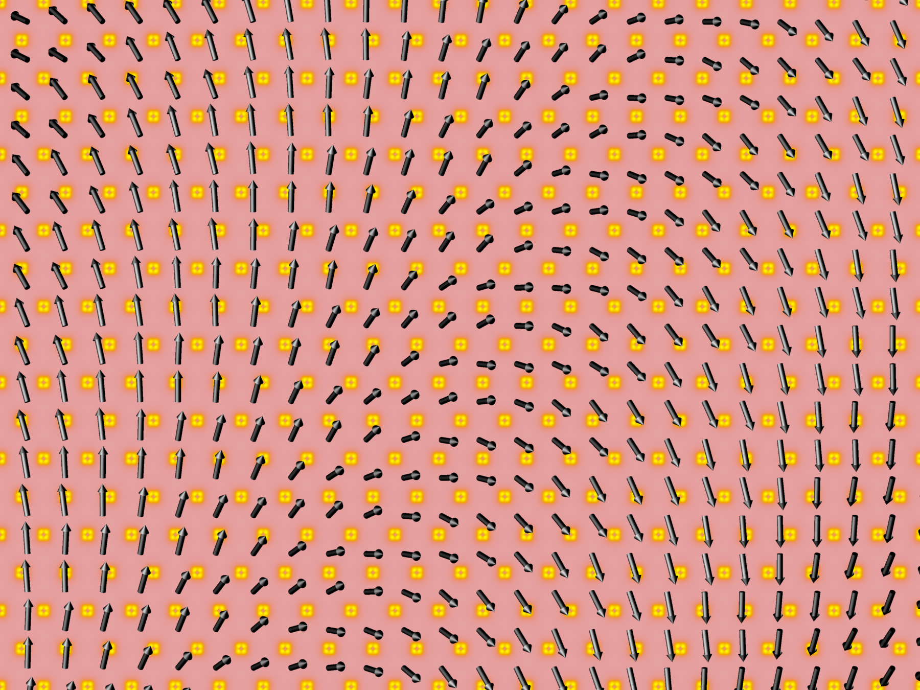
(a)

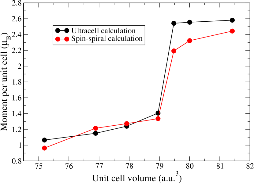
(b)

Figure 2: (a) Ultra long-range magnetization density of $\gamma$-Fe plotted in the plane perpendicular to $[001]$. The color indicates the magnitude of the magnetization and the arrows indicate direction. The modulation encompasses 32 unit cells in the $[100]$ direction. (b) Plot of moment against unit cell volume for both the long-range and spin-spiral ansatz.

The first numerical test deals with the so called $\gamma$ phase of Fe. Previous calculationsSjöstedt and Nordström (2002) have shown that the spin-spiral state has the lowest energy compared to several commensurate ferromagnetic and anti-ferromagnetic structures. The ultra long-range method allows us to address the question whether the much larger variation freedom associated with ultra-cell still yields the spin-spiral as ground state. We performed a traditional spin-spiral calculation and an ultra-cell calculation for this materials. The parameters used are as follows: Ultracell ${\bf k}$-point grid: $1\times 12\times 12$, ${\bf Q}$-point grid: $32\times 1\times 1$, ultracell: $32\times 1\times 1$ unit cells. A single unit cell was used for the spin-spiral calculation with a $12\times 12\times 12$ ${\bf k}$-point grid and a ${\bf Q}$-vector of $1/32$.

An initial magnetic field is required to break the spin symmetry. To ensure an unbiased calculation, we applied a random field to the ultracell calculation and subsequently reduced it to zero. Throughout the calculation, we enforced the constraint $\int_{\rm unit}d^{3}r\,{\bf m}_{{\bf Q}=0}({\bf r})=0$. This ensures that the system is not drawn to a lattice-periodic ferromagnetic solution. The magnetization converged to an ordered state where the magnitude was constant over the ultracell and only the direction varied (Fig. 2(a)). This corresponds precisely to the spin-spiral state i.e. the ultra-cell calculations shows that the spin-spiral state is still the lowest energy solution. The overall magnitude of the magnetization is sensitive to the lattice parameter and undergoes a transition from $\sim 1\mu_{B}$ to $\sim 2.5\mu_{B}$ for this relatively small ${\bf Q}$-vector. As may be seen in Fig. 2(b), this behavior is observed for both the ultracell and spin-spiral calculations.

IV.2 Spin density wave in bcc Cr

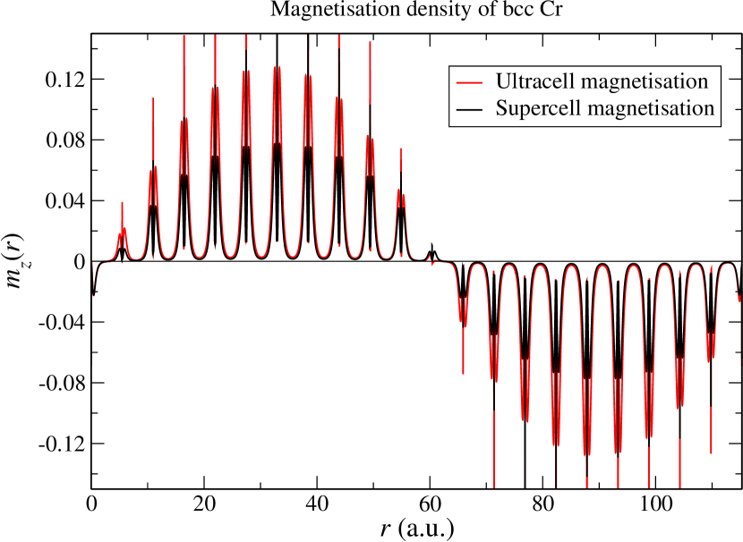
(a)

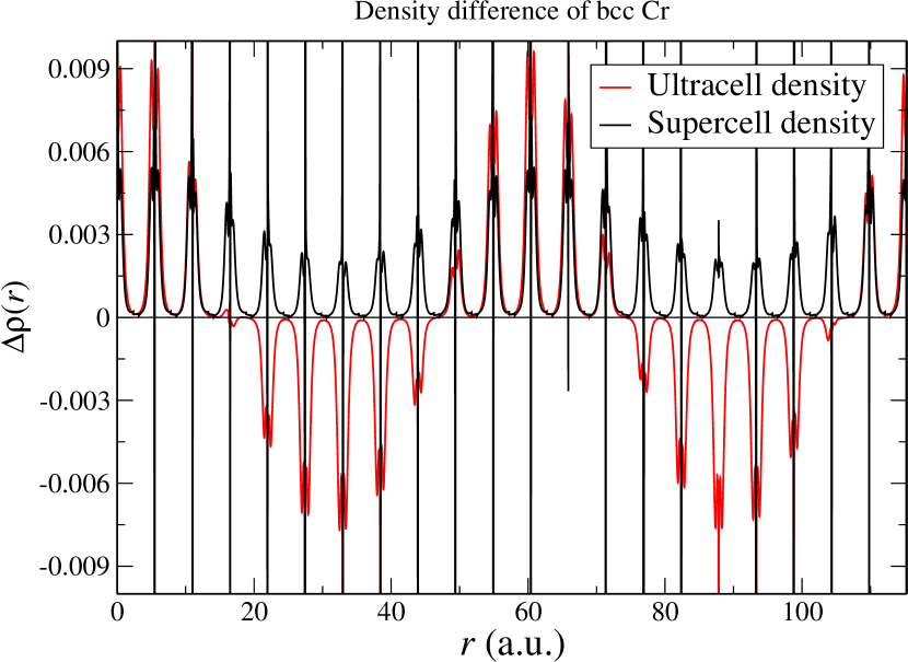
(b)

Figure 3: (a) Magnetization density for bcc Cr over 21 unit cells. (b) Change in density over the same range. For the ultracell, this was generated by setting $\rho_{{\bf Q}=0}({\bf r})$ in Eq. (7) to zero. For the super-cell, the lattice-periodic density was subtracted leaving just the modulated density.

In a second test, we aim at calculating the spin density wave (SDW) state in Cr. The existence of a SDW in Cr is well known and the first research dates back to around 1960 Corliss et al. (1959); Bykov et al. (1960); Overhauser (1962). Despite this, computing the SDW state within DFT remains difficult and has been the topic of many studies Moruzzi et al. (1978); Kübler (1980); L Skriver (1981); I Kulikov and Kulatov (1082); Kulikov et al. (1987); Chen et al. (1988); Moruzzi and Marcus (1992); Singh and Ashkenazi (1992); Hirai (1997); Guo and Wang (2000); Bihlmayer et al. (2000); Schäfer et al. (2000); Hafner et al. (2001), with partially conflicting results Cottenier et al. (2002). It is likely that a SDW is not the true ground state of Cr within DFT Hafner et al. (2002), however we will not focus here on the inherent complexities of the system. This state is not achievable by the spin-spiral ansatz because the magnitude of the moment changes but not its direction, thus a super-cell calculation is required. Cr is an excellent test scenario, as the periodicity of the SDW is $\sim 20.83$ unit cells, which is still well within computational reach of the super-cell approach.

For our comparison, we use the LSDA and a lattice parameter of $2.905\text{\,}\mathrm{\SIUnitSymbolAngstrom}$ as suggested by Cottenier et al.Cottenier et al. (2002). We consider $21\times 1\times 1$ unit cells of bulk Cr for both super-cell and ultracell calculations. For the super-cell we used a $1\times 12\times 12$ ${\bf k}$-point grid. A randomized symmetry breaking magnetic field was used to start the calculation and subsequently reduced to zero. Spin-orbit coupling is also included. Our super-cell calculation reproduces the result by Cottenier et al.Cottenier et al. (2002). For the ultracell we also used a $1\times 12\times 12$ ${\bf k}$-point grid with a $21\times 1\times 1$ ${\bf Q}$-points grid corresponding to a grid of $11\times 1\times 1$ $\bm{\kappa}$-points to obtain the best possible sampling of the xc-potential and -field. Around 60 empty states in the lattice-periodic basis are used to provide enough degrees of freedom during the convergence. We started with a randomized initial field that was reduced after each step. Throughout the calculation, we enforced the constraint $\int_{\rm MT}d^{3}r\,{\bf m}_{{\bf Q}=0}({\bf r})=0$ for each muffin-tin. This ensures that the system is not drawn to a lattice-periodic anti-ferromagnetic solution.

Our results are shown in Fig. 3. Specifically, Fig. 3(a) shows the comparison of the magnetization in the SDW state, as obtained from the super-cell and ultracell calculations. The maximum moment of the ultracell calculations is larger than that of the super-cell, 1.174 $\mu_{B}$ and 0.712 $\mu_{B}$, respectively. This we attribute to the fact that the ultra long-range calculation is performed in the basis of Kohn-Sham states and not in the original LAPW basis for which the linearization energies are optimally adjusted. It is also known that LSDA calculations this of system are particularly sensitive to the basis and the moment depends strongly on the lattice parameterCottenier et al. (2002).

In Fig. 3(b) we present the charge density wave (CDW) which is known to stabilize alongside the SDW with twice the period. While obtaining the CDW in the ultracell is straight-forward (as all $\rho_{\bf Q}({\bf r})$ are known), it is numerically more challenging to extract it for the super-cell. We did this by subtracting the density from the calculation of a single unit cell. We obtain the same periodicity in both calculations as well as a comparable magnitude.

IV.3 Saw-tooth potential in Si

(a)

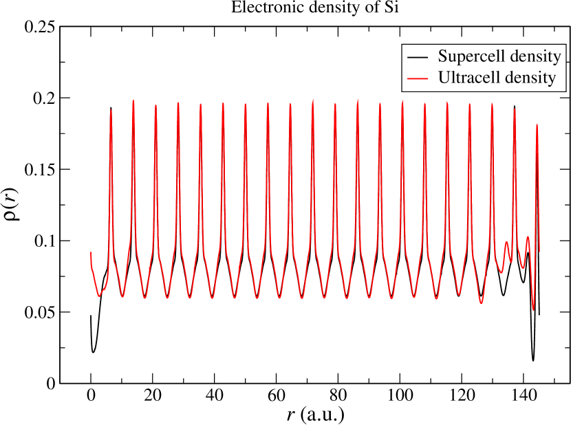
(b)

Figure 4: (a) Saw-tooth potential applied to 20 unit cells of silicon in the ultracell and super-cell. The ultracell potential is smoother than that of the super-cell because of the relatively small number of ${\bf Q}$ vectors used to expand it. (b) The resultant ground state density in the ultracell and super-cell. This was plotted along a line which was slightly off-set from the atomic centers in order to avoid the very high densities near the nuclei.

The previous two examples involved modulations in long-range magnetic order, but we also need to test the method with long-range, external electrostatic fields. This is in anticipation of a future development where ultra long-range TDDFT calculations are performed in conjunction with Maxwell’s equations. In such a scenario, an electromagnetic wave propagating through the solid could have a periodicity of many hundreds of unit cells. The long-range ansatz should be ideal for performing such a simulation. With that goal in mind, we apply a simple saw-tooth potential to silicon over a range of 20 unit cells to check if the ultracell calculation agrees with its super-cell equivalent. This corresponds to a constant electric field, at least near the center of the saw-tooth. Both calculations were performed with a $4\times 4\times 4$ ${\bf k}$-point grid. The ultracell calculation used a ${\bf Q}$-point grid of $20\times 1\times 1$ with a basis of 60 empty states per ${\bf k}$-point. The applied electric field was $0.01$ in atomic units and the corresponding saw-tooth potential is plotted in Fig. 4(a). As can been seen, there is a difference between the ultracell and super-cell potentials. The ultracell potential is expanded in a finite set of ${\bf Q}$ vectors and thus contains oscillations on the length scale of the longest vector. The super-cell potential is a sharp saw-tooth. Despite this difference, the two densities plotted in Fig. 4(b) are broadly the same with strong screening near the center and charge accumulation and depletion near the edges. We note that for the intended purpose of describing propagating light through solids, the resulting electric and magnetic fields will be well expanded with a finite number of ${\bf Q}$ vectors.

IV.4 Long-range electrostatic potential in LiF

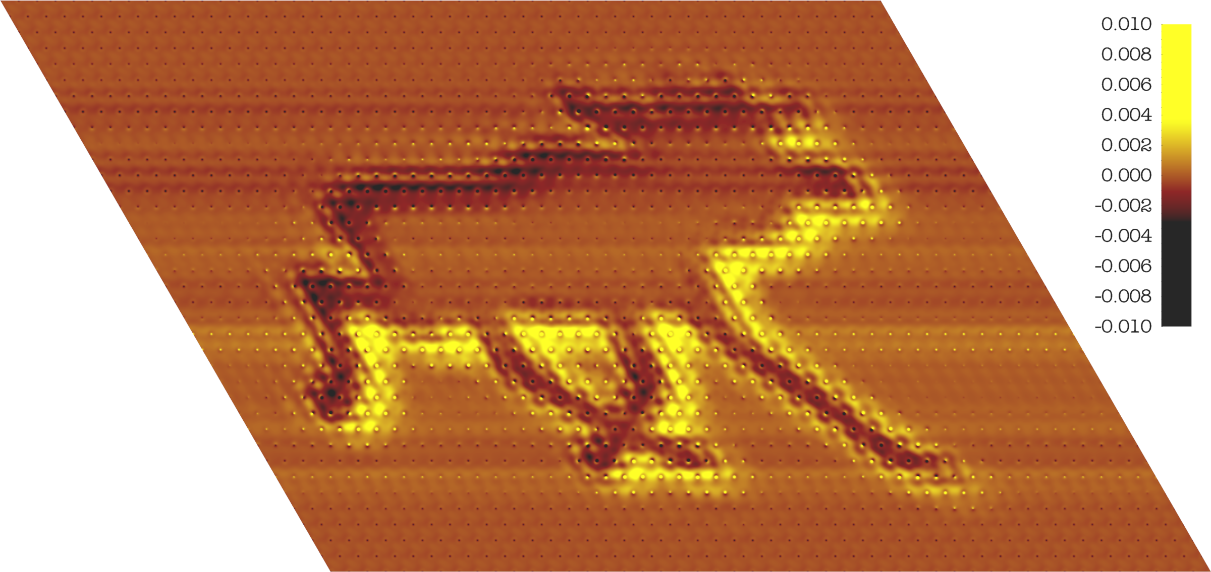
Figure 5: Self-consistent density without the $\rho_{{\bf Q}=0}({\bf r})$ term for a 3456 atom ultracell of LiF with an artificial external potential. The plotting plane is perpendicular to $[001]$ and contains $48\times 36$ unit cells.

Lastly we perform a calculation which is too large for a super-cell. Rather than attempting to model a physical phenomenon at this stage, we simply apply an arbitrarily chosen electrostatic potential to an insulator, in this case LiF. An ultracell of $48\times 36\times 1$ unit cells was constructed with an equivalent ${\bf Q}$-point grid. The number of empty states per ${\bf k}$-point was taken to be 4 to keep the memory requirements to within those of our computer. The resultant change in density away from unit cell periodicity is plotted in Fig. 5. As the potential is artificial, the important metric here is the computational effort expended in reaching the self-consistent solution. The rate of convergence is fairly slow because of the effect of the long-range Coulomb interaction, and thus we performed 170 iterations of the self-consistent loop. The calculation was performed on 480 CPU cores and each iteration took about 40 minutes. This level of performance for an all-electron calculation indicates that physical phenomena involving modulations of the electronic state over hundreds or thousands of unit cells are within reach of this approach.

V Conclusion and outlook

We have developed a method which makes possible the ab-initio treatment of hitherto uncomputable length-scales in solids. This consists of a modified Bloch ansatz and a set of Kohn-Sham equations which have to be solved self-consistently. The underlying lattice of nuclear charges is still periodic on the unit cell length scale but the electronic state can accommodate arbitrary modulations on any length scale. Based on our experience with the all-electron Elk code, we are confident that this method can be efficiently implemented in most existing solid-state electronic structure codes. We demonstrated the capabilities of the novel method by solving an arbitrary external potential applied to nearly 3500 atoms of LiF. Additionally, we showed that our method can reproduce the results obtained by super-cell calculations on smaller length scales for both insulators and magnetic solids. The method presented in this paper opens up exciting possibilities of future research: on the technical level, a derivation of long-range and explicitly ${\bf Q}$-dependent xc-potentials (see, for example, Pellegrini et al. Pellegrini et al. (2020)). On the applied level, our method could pave the way to calculations of mesoscopic systems, such as magnetic domain walls or skyrmions, which have so far been out of reach for ab-initio methods like DFT. Furthermore, the novel technique is straightforwardly incorporated in real-time TDDFT calculations which, when combined with the solution of Maxwell’s equations, will give access to the propagation of electromagnetic radiation through extended solids within a genuine ab-initio description.

Acknowledgments: SS and TM would like to thank DFG for funding though QUTIF project. EKUG acknowledges financial support by European Research Council Advanced Grant Fact (ERC-2017-AdG-788890).

References

- Hohenberg and Kohn (1964) P. Hohenberg and W. Kohn, Phys. Rev. 136, B864 (1964).
- von Barth and Hedin (1972) U. von Barth and L. Hedin, Journal of Physics C: Solid State Physics 5, 1629 (1972).
- Vignale and Rasolt (1987) G. Vignale and M. Rasolt, Phys. Rev. Lett. 59, 2360 (1987).
- Oliveira et al. (1988) L. N. Oliveira, E. K. U. Gross, and W. Kohn, Phys. Rev. Lett. 60, 2430 (1988).
- Runge and Gross (1984) E. Runge and E. K. U. Gross, Phys. Rev. Lett. 52, 997 (1984).
- Goedecker (1999) S. Goedecker, Rev. Mod. Phys. 71, 1085 (1999).
- Sandratskii (1986) L. M. Sandratskii, physica status solidi (b) 136, 167 (1986).
- Weinert (1981) M. Weinert, Journal of Mathematical Physics 22, 2433 (1981).
- Pellegrini et al. (2020) C. Pellegrini, T. Müller, J. K. Dewhurst, S. Sharma, A. Sanna, and E. K. U. Gross, Phys. Rev. B 101, 144401 (2020).
- (10) “The Elk Code,” http://elk.sourceforge.net/.
- Sjöstedt and Nordström (2002) E. Sjöstedt and L. Nordström, Phys. Rev. B 66, 014447 (2002).
- Corliss et al. (1959) L. M. Corliss, J. M. Hastings, and R. J. Weiss, Phys. Rev. Lett. 3, 211 (1959).
- Bykov et al. (1960) V. N. Bykov, V. S. Golovkin, N. V. Ageev, V. A. Levdik, and S. I. Vinogradov, Soviet Physics Doklady 4, 1070 (1960).
- Overhauser (1962) A. W. Overhauser, Phys. Rev. 128, 1437 (1962).
- Moruzzi et al. (1978) V. Moruzzi, J. Janak, and A. Williams, Calculated Electronic Properties of Metals, edited by V. Moruzzi, J. Janak, and A. Williams (Pergamon, 1978) pp. 30 – 159.
- Kübler (1980) J. Kübler, Journal of Magnetism and Magnetic Materials 20, 277 (1980).
- L Skriver (1981) H. L Skriver, Journal of Physics F: Metal Physics 11, 97 (1981).
- I Kulikov and Kulatov (1082) N. I Kulikov and E. Kulatov, Journal of Physics F: Metal Physics 12, 2291 (1082).
- Kulikov et al. (1987) N. I. Kulikov, M. Alouani, M. A. Khan, and M. V. Magnitskaya, Phys. Rev. B 36, 929 (1987).
- Chen et al. (1988) J. Chen, D. Singh, and H. Krakauer, Phys. Rev. B 38, 12834 (1988).
- Moruzzi and Marcus (1992) V. L. Moruzzi and P. M. Marcus, Phys. Rev. B 46, 3171 (1992).
- Singh and Ashkenazi (1992) D. J. Singh and J. Ashkenazi, Phys. Rev. B 46, 11570 (1992).
- Hirai (1997) K. Hirai, Journal of the Physical Society of Japan 66, 560 (1997).
- Guo and Wang (2000) G. Y. Guo and H. H. Wang, Phys. Rev. B 62, 5136 (2000).
- Bihlmayer et al. (2000) G. Bihlmayer, T. Asada, and S. Blügel, Phys. Rev. B 62, R11937 (2000).
- Schäfer et al. (2000) J. Schäfer, E. Rotenberg, S. Kevan, and P. Blaha, Surface Science 454-456, 885 (2000).
- Hafner et al. (2001) R. Hafner, D. Spisák, R. Lorenz, and J. Hafner, Journal of Physics: Condensed Matter 13, L239 (2001).
- Cottenier et al. (2002) S. Cottenier, B. De Vries, J. Meersschaut, and M. Rots, J. Phys.: Condens. Matter 14, 3275 (2002).
- Hafner et al. (2002) R. Hafner, D. Spišák, R. Lorenz, and J. Hafner, Phys. Rev. B 65, 184432 (2002).