Angular displacements estimation enhanced by squeezing and parametric amplification

Abstract

We theoretically study the angular displacements estimation based on a modified Mach-Zehnder interferometer (MZI), in which two optical parametric amplifiers (PAs) are introduced into two arms of the standard MZI, respectively. The employment of PAs can both squeeze the shot noise and amplify the photon number inside the interferometer. When the unknown angular displacements are introduced to both arms, we derive the multiparameter quantum Cramér-Rao bound (QCRB) using the quantum Fisher information matrix approach, and the bound of angular displacements difference between the two arms is compared with the sensitivity of angular displacement using the intensity detection. On the other hand, in the case where the unknown angular displacement is in only one arm, we give the sensitivity of angular displacement using the method of homodyne detection. It can surpass the standard quantum limit (SQL) and approach the single parameter QCRB. Finally, the effect of photon losses on sensitivity is discussed.

1 Introduction

Phase estimation illustrates well the advantages of quantum metrology, with a wide range of applications[1, 2, 3, 4, 5]. As fundamental devices, a number of interferometer configurations have been proposed for phase estimation. One common configuration is the SU(2) interferometer, e.g., a Mach-Zehnder interferometer (MZI), consists of two linear beam splitters (BSs). The sensitivity of these interferometers is limited by the vacuum fluctuation entering from the unused input port. To further enhance measurement sensitivity, another commonly used configuration is proposed by Yurke et al.[6], known as the SU(1,1) interferometer, in which optical parametric amplifiers (PAs) or four-wave mixers are employed as the wave splitting and recombination elements. Because the signal is amplified while the noise level is kept close to the shot noise limit, these types of interferometers have been extensively studied both in theory[7, 8, 9, 10, 11, 12, 13, 14, 15, 16, 17] and experiment[18, 19, 20, 21, 22, 23, 24, 25, 26]. Besides the above, the interferometers with novel structures have emerged in large numbers. Kong et al.[27] proposed a scheme of PA+BS, and it can also beat the SQL of phase sensitivity by a similar amount for SU(1,1) interferometer. Szigeti et al.[28] presented a pumped-up interferometer where all the input particles participate in the phase measurement. Anderson et al.[29] constructed a truncated SU(1,1) interferometer in which the second nonlinear interaction is replaced with balanced homodyne detection. More recently, Du et al.[30] reported a SU(2)-in-SU(1,1) nested interferometer, which combines advantages of SU(1,1) and SU(2) interferometry. Zuo et al.[31] proposed and experimentally demonstrated a compact quantum interferometer combining squeezing and parametric amplification.

Besides the phase estimation, the angular displacement estimation has been another topic of interest with a number of potential applications, including rotational control of microscopic systems [32], detecting spinning objects [33] and exploration of effects such as the rotational Doppler shift [34], and so on [35, 36]. The use of light endowed with orbital angular momentum (OAM) can improve the sensitivity of the angular displacement measurement, which amplifies an angular displacement $\theta$ to $l\theta$ [37], where $l$ denotes topological charge and can take any integer value. Recently, some interferometer configurations have been utilized to realize precision measurement of angular displacement. Jha et al.[38] showed that the sensitivity of angular displacement in MZI can reach $\frac{1}{2l\sqrt{N}}$ and $\frac{1}{2lN}$ by employing $N$-unentangled photons and $N$-entangled photons, respectively. Liu et al.[39] analyzed the sensitivity of angular displacement based on an SU(1,1) interferometer. Zhang et al.[40] investigated angular displacement estimation via the scheme of PA+BS. In addition, some estimation protocols using other inputs and detection strategies are studied[41, 42, 43]. Based on the modified MZI[31], we can obtain the higher sensitivity of angular displacement for the case of angular displacement only in one arm. Furthermore, if two angular displacements are introduced to both arms, no researchers have studied this situation from the multiparameter estimation perspective so far.

In this paper, we study the estimation of angular displacements based on a modified MZI. The multiparameter quantum Cramér-Rao bound (QCRB) is derived using the method of quantum Fisher information matrix (QFIM), and the bound of angular displacements difference between the two arms is compared with the sensitivity of angular displacement using the intensity detection. For the angular displacement is only in one arm, the QCRB of angular displacement is compared with the sensitivity of the homodyne detection method.

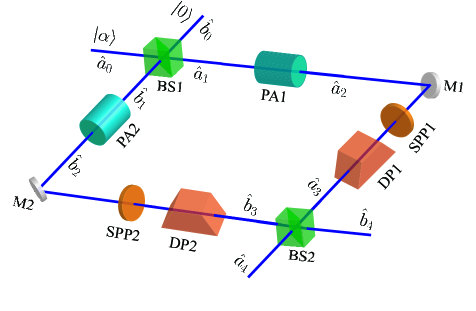
Figure 1: Two sets of optical parametric amplifiers (PAs), spiral phase plates (SPPs) and Dove prisms (DPs) are placed in two arms of the standard MZI, respectively. The squeezed states generated from the PAs are directly used for the probe states. The optical field passing through the SPP and DP will have a phase shift of $2l\theta$, where $l$ denotes topological charge and $\theta$ is the rotation angle of a Dove prism. $\hat{a}_{i}$ and $\hat{b}_{i}$ ($i=0,1,2,3,4$) denote light beams in the different processes. $\mathrm{M}$: mirrors; $\mathrm{BS}$: beam splitters.

2 Model

Different from the usual MZI, two sets of PAs, spiral phase plates (SPPs) and Dove prisms (DPs) are placed in two arms of the MZI, respectively, as shown in Fig. 1. A coherent state $|\alpha\rangle$ ($\alpha=|\alpha|$) and a vacuum state are injected into the interferometer. $\hat{b}_{0}$ is in vacuum state, $\hat{a}_{i}$ and $\hat{b}_{i}$ ($i=0,1,2,3,4$) denote light fields in the different processes. The SPP is used to introduce the OAM degree of freedom, i.e. the light field passing through the SPP will carry OAM. The employment of DP transforms the topological charge from $l$ to $-l$ and imposes a phase shift of $2l\theta$ to the field, where $\theta$ is the rotation angle of the DP and the parameter to be estimated in this paper.

The input-output relation of the first beam splitter is given by

$$\hat{a}_{1}=\sqrt{T}\hat{a}_{0}-\sqrt{R}\hat{b}_{0},\hat{b}_{1}=\sqrt{R}\hat{a}_{0}+\sqrt{T}\hat{b}_{0},$$ (1)

where $R$ and $T$ are the reflectivity and transmissivity of the BS, respectively. The PAs located in each arm are used for squeezing the shot noise and amplifying the internal photon number. The relationship between input and output is

$$\hat{a}_{2}=\cosh r\hat{a}_{1}+\sinh r\hat{a}_{1}^{\dagger},\hat{b}_{2}=\cosh r\hat{b}_{1}+\sinh r\hat{b}_{1}^{\dagger},$$ (2)

where $r$ is the squeezing factor of PAs. The optical field passing through the SPP and DP is described as

$$\hat{a}_{3}=\hat{a}_{2}e^{2il\theta_{a}},\hat{b}_{3}=\hat{b}_{2}e^{2il\theta_{b}},$$ (3)

where $\theta_{a}$ and$\ \theta_{b}$ correspond to the rotation angles of the DP1 and DP2, respectively. The full input-output relation of the scheme is given by

$$\hat{a}_{4} =(Te^{2il\theta_{a}}+Re^{2il\theta_{b}})(\cosh r\hat{a}_{0}+\sinh r\hat{a}_{0}^{\dagger})$$

$$+\sqrt{TR}(e^{2il\theta_{b}}-e^{2il\theta_{a}})(\cosh r\hat{b}_{0}+\sinh r\hat{b}_{0}^{\dagger}),$$

$$\hat{b}_{4} =(Te^{2il\theta_{b}}+Re^{2il\theta_{a}})(\cosh r\hat{b}_{0}+\sinh r\hat{b}_{0}^{\dagger})$$

$$+\sqrt{TR}(e^{2il\theta_{b}}-e^{2il\theta_{a}})(\cosh r\hat{a}_{0}+\sinh r\hat{a}_{0}^{\dagger}).$$ (4)

3 Angular displacements estimation

3.1 Angular displacements in both arms

In this section, we consider a general situation in which $\theta_{d}$ and $\theta_{s}$ are the parameters to be estimated, where $\theta_{d}=\theta_{b}-\theta_{a}$, $\theta_{s}=\theta_{b}+\theta_{a}$. Such a kind of problem can be dealt with by the multiparameter quantum estimation theory. The bounds of the angular displacement estimation uncertainties can be obtained by the quantum Cramér-Rao inequality[44, 45, 46]:

$$\Sigma(\theta_{1},\theta_{2})\geq\mathcal{F}^{-1}(\theta_{1},\theta_{2}),$$ (5)

where $\Sigma$ is the covariance matrix for parameters $\theta_{1}$, $\theta_{2}$, $\mathcal{F}^{-1}$ is the inverse matrix of the QFIM $\mathcal{F}(\theta_{1},\theta_{2})$ with elements $\mathcal{F}_{ij}$ ($i,j=1,2$) given by

$$\mathcal{F}_{ij}=\mathrm{Tr}\left[\rho(\theta_{1},\theta_{2})\frac{\hat{L}_{i}\hat{L}_{j}+\hat{L}_{j}\hat{L}_{i}}{2}\right],$$ (6)

in which $\rho$ is the density matrix of the system and the symmetrized logarithmic derivatives $\hat{L}_{i}$ defined by

$$\frac{\partial\rho(\theta_{1},\theta_{2})}{\partial\theta_{i}}=\frac{\rho\hat{L}_{i}+\hat{L}_{i}\rho}{2}.$$ (7)

For the case of unitary evolution of a pure initial state, the QFIM can be caiculated analytically,

$$\mathcal{F}_{ij}=4\operatorname{Re}(\langle\partial_{i}\psi_{\theta}|\partial_{j}\psi_{\theta}\rangle-\langle\partial_{i}\psi_{\theta}|\psi_{\theta}\rangle\langle\psi_{\theta}|\partial_{j}\psi_{\theta}\rangle),$$ (8)

where $|\psi_{\theta}\rangle$ is the state vector after evolving through DP and $|\partial_{i}\psi_{\theta}\rangle=\partial|\psi_{\theta}\rangle/\partial\theta_{i}$.

For the estimation of $\theta_{d}$ and $\theta_{s}$, the QFIM is given by

$$\mathcal{F}(\theta_{d},\theta_{s})=\left(\begin{array}[c]{cc}F_{dd}&F_{{ds}}\\ F_{sd}&F_{ss}\end{array}\right),$$ (9)

where the subscripts $d$ and $s$ denote $\theta_{d}$ and $\theta_{s}.$ Using Eq. (8) and Eq. (4), the matrix elements take the form

$$F_{dd} =4l^{2}[\langle(\hat{n}_{b_{2}}-\hat{n}_{a_{2}})^{2}\rangle-\langle\hat{n}_{b_{2}}-\hat{n}_{a_{2}}\rangle^{2}]$$

$$=4l^{2}(\left|\alpha\right|^{2}e^{4r}+\sinh^{2}2r),$$

$$F_{ds} =4l^{2}[\langle(\hat{n}_{b_{2}}-\hat{n}_{a_{2}})(\hat{n}_{b_{2}}+\hat{n}_{a_{2}})\rangle-\langle\hat{n}_{b_{2}}-\hat{n}_{a_{2}}\rangle\langle\hat{n}_{b_{2}}+\hat{n}_{a_{2}}\rangle]$$

$$=4l^{2}\left|\alpha\right|^{2}e^{4r}(1-2T),$$

$$F_{sd} =4l^{2}[\langle(\hat{n}_{b_{2}}+\hat{n}_{a_{2}})(\hat{n}_{b_{2}}-\hat{n}_{a_{2}})\rangle-\langle\hat{n}_{b_{2}}+\hat{n}_{a_{2}}\rangle\langle\hat{n}_{b_{2}}-\hat{n}_{a_{2}}\rangle]$$

$$=4l^{2}\left|\alpha\right|^{2}e^{4r}(1-2T),$$

$$F_{ss} =4l^{2}[\langle(\hat{n}_{b_{2}}+\hat{n}_{a_{2}})^{2}\rangle-\langle\hat{n}_{b_{2}}+\hat{n}_{a_{2}}\rangle^{2}]$$

$$=4l^{2}(\left|\alpha\right|^{2}e^{4r}+\sinh^{2}2r),$$ (10)

where $\hat{n}_{a_{2}}=\hat{a}_{2}^{\dagger}\hat{a}_{2}$, $\hat{n}_{b_{2}}=\hat{b}_{2}^{\dagger}\hat{b}_{2}$. Then the corresponding bounds are given by

$$\Delta^{2}\theta_{d} \geq\frac{F_{ss}}{F_{dd}F_{ss}-F_{ds}F_{sd}},$$

$$\Delta^{2}\theta_{s} \geq\frac{F_{dd}}{F_{dd}F_{ss}-F_{ds}F_{sd}}.$$ (11)

As seen in Eq. (11), in general, the bound for estimating $\theta_{d}$ depends on the information amount of $\theta_{s}$ due to the nonzero off-diagonal elements in the QFIM. When $R=T=1/2$, $F_{ds}=F_{sd}=0$, then Eq. (11) is reduced to

$$\Delta^{2}\theta_{d} \geq\frac{1}{F_{dd}},$$

$$\Delta^{2}\theta_{s} \geq\frac{1}{F_{ss}},$$ (12)

which means that one does not need to consider if $\theta_{s}$ is known to find the ultimate bound of $\theta_{d}$.

The QFI is the intrinsic information in the quantum state and is not related to the actual measurement procedure. It characterizes the maximum amount of information that can be extracted from quantum experiments about an unknown parameter using the best (and ideal) measurement device. Here, we consider the intensity detection as our measurement strategy, and compare the bound of $\theta_{d}$ in Eq. (12) with the sensitivity using the intensity detection.

The sensitivity is obtained through an error propagation analysis

$$\Delta\theta=\frac{(\Delta^{2}\hat{O})^{1/2}}{|\partial\langle\hat{O}\rangle/\partial\theta|},$$ (13)

where $\Delta^{2}\hat{O}$ and $|\partial\langle\hat{O}\rangle/\partial\theta_{d}|$ denote the noise of observable $\hat{O}$ and its rate of change with respect to $\theta$, respectively. The detected variable $\hat{O}$ can be phase quadrature or the photon number. Here, we use the difference in the intensities of the two output ports as the detection variable, that is

$$\hat{N} =\hat{a}_{4}^{\dagger}\hat{a}_{4}-\hat{b}_{4}^{\dagger}\hat{b}_{4}=\mathcal{A}\hat{T}_{1}+\mathcal{B}\hat{T}_{2}+\mathcal{B}^{\ast}\hat{T}_{2}^{\dagger}-\mathcal{A}\hat{T}_{3},$$ (14)

where

$$\mathcal{A} =(T-R)^{2}+4TR\cos(2l\theta_{d}),\mathcal{B}=2\sqrt{TR}(R-Re^{-2il\theta_{d}}+Te^{2il\theta_{d}}-T),$$

$$\hat{T}_{1} =\cosh^{2}r\hat{a}_{0}^{\dagger}\hat{a}_{0}+\cosh r\sinh r\hat{a}_{0}^{\dagger 2}+\cosh r\sinh r\hat{a}_{0}^{2}+\sinh^{2}r\hat{a}_{0}\hat{a}_{0}^{\dagger},$$

$$\hat{T}_{2} =\cosh^{2}r\hat{a}_{0}^{\dagger}\hat{b}_{0}+\cosh r\sinh r\hat{a}_{0}^{\dagger}\hat{b}_{0}^{\dagger}+\cosh r\sinh r\hat{a}_{0}\hat{b}_{0}+\sinh^{2}r\hat{a}_{0}\hat{b}_{0}^{\dagger},$$

$$\hat{T}_{3} =\cosh^{2}r\hat{b}_{0}^{\dagger}\hat{b}_{0}+\cosh r\sinh r\hat{b}_{0}^{\dagger 2}+\cosh r\sinh r\hat{b}_{0}^{2}+\sinh^{2}r\hat{b}_{0}\hat{b}_{0}^{\dagger}.$$ (15)

Under the condition of $R=T=1/2$, the sensitivity of angular displacement can be written as

$$\Delta\theta_{d}^{\mathrm{ID}}=\frac{\sqrt{|\alpha|^{2}[\cos^{2}(2l\theta_{d})e^{4r}+\sin^{2}(2l\theta_{d})]+\sinh^{2}(2r)\cos^{2}(2l\theta_{d})}}{2l|\alpha|^{2}e^{2r}|\sin(2l\theta_{d})|}.$$ (16)

where the superscript $\mathrm{ID}$ denotes the intensity detection. When $2l\theta_{d}=\pi/2$, the optimal sensitivity is

$$\Delta\theta_{d_{optimal}}^{\mathrm{ID}}=\frac{1}{2l|\alpha|e^{2r}}.$$ (17)

Compared with the bound for estimating $\theta_{d}$ in Eq. (12), we find that when the intensity of the input coherent state is strong enough, $\Delta\theta_{d_{optimal}}^{\mathrm{ID}}\approx\Delta\theta_{d}$, i.e. the optimal sensisitivity using the intensity detection can saturate the corresponding QCRB.

3.2 Angular displacement in one arm

In the preceding section, we considered a two-parameter estimation problem and used the QFIM approach to calculate the QCRB of the angular displacements. Now we assume $R=T=1/2$, $\theta_{a}=0$ and calculate the single parameter QCRB. For the single parameter estimation, the QCRB according to the QFI is given by [46]

$$\Delta\theta_{\mathrm{QCRB}}=\frac{1}{\sqrt{\mathcal{F}}}.$$ (18)

Eq. (6) is simplified to

$$\mathcal{F}=\mathrm{Tr}[\rho(\theta)L^{2}],$$ (19)

where the corresponding symmetrized logarithmic derivatives $L$ defined by

$$\frac{\partial\rho(\theta)}{\partial\theta}=\frac{\rho L+L\rho}{2}.$$ (20)

Under the lossless condition, for a pure state, the QFI is reduced to

$$\mathcal{F}=4(\langle\partial_{\theta}\psi_{\theta}|\partial_{\theta}\psi_{\theta}\rangle-|\langle\partial_{\theta}\psi_{\theta}|\psi_{\theta}\rangle|^{2}),$$ (21)

where $|\psi_{\theta}\rangle$ is the state vector after evolving through DP and $|\partial_{\theta}\psi_{\theta}\rangle=\partial|\psi_{\theta}\rangle/\partial\theta$. In our case, the QFI is given by

$$\mathcal{F}=16l^{2}\left[\langle\hat{n}_{b_{2}}^{2}\rangle-\langle\hat{n}_{b_{2}}\rangle^{2}\right]=8l^{2}(e^{4r}\left|\alpha\right|^{2}+\sinh^{2}2r).$$ (22)

Using Eq. (18), the QCRB is

$$\Delta\theta_{\mathrm{QCRB}}=\frac{1}{2\sqrt{2}l\sqrt{e^{4r}\left|\alpha\right|^{2}+\sinh^{2}2r}}.$$ (23)

Then we analyze the measurement sensitivity of angular displacement $\theta$ ($\theta=\theta_{b}$) using the balanced homodyne detection. The measurement operator is

$$\hat{Y}_{b_{4}}=-i(\hat{b}_{4}-\hat{b}_{4}^{\dagger}).$$ (24)

When $R=T=1/2$ and $\theta_{a}=0$, Eq. (4) can be written as

$$\hat{a}_{4} =[(e^{2il\theta}+1)(\cosh r\hat{a}_{0}+\sinh r\hat{a}_{0}^{\dagger})+(e^{2il\theta}-1)(\cosh r\hat{b}_{0}+\sinh r\hat{b}_{0}^{\dagger})]/2,$$

$$\hat{b}_{4} =[(e^{2il\theta}+1)(\cosh r\hat{b}_{0}+\sinh r\hat{b}_{0}^{\dagger})+(e^{2il\theta}-1)(\cosh r\hat{a}_{0}+\sinh r\hat{a}_{0}^{\dagger})]/2.$$ (25)

The rate of change of $\langle\hat{Y}_{b_{4}}\rangle$ with respect to $\theta$ and the variance of $\hat{Y}_{b_{4}}$ is given by

$$|\partial_{\theta}\langle\hat{Y}_{b_{4}}\rangle|=2l(\cosh r+\sinh r)|\alpha\cos(2l\theta)|,$$ (26)

and

$$\Delta^{2}\hat{Y}_{b_{4}}=-\sinh r\cosh r[\cos(4l\theta)+1]+\cosh(2r),$$ (27)

respectively. Using error propagation formula, the sensitivity is

$$\Delta\theta^{\mathrm{BHD}}=\frac{\sqrt{-\sinh r\cosh r[\cos(4l\theta)+1]+\cosh(2r)}}{2l(\cosh r+\sinh r)|\alpha\cos(2l\theta)|},$$ (28)

where the superscript $\mathrm{BHD}$ denotes the balanced homodyne detection.

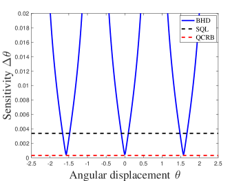
Figure 2: The sensitivity as a function of angular displacement $\theta$ in the case of $l=1$, $r=2$ and $|\alpha|=20$.

Fig. 2 shows the behavior of $\Delta\theta^{\mathrm{BHD}}$ as a function of $\theta$. This result shows that the sensitivity of balanced homodyne detection can surpass the SQL and approach the QCRB. When $2l\theta=k\pi$ ($k$ is an arbitrary integer), the fluctuation of $\hat{Y}_{b_{4}}$ is reduced to $e^{-2r}$ and the optimal sensitivity is obtained

$$\Delta\theta_{optimal}^{\mathrm{BHD}}=\frac{\cosh r-\sinh r}{2l(\cosh r+\sinh r)|\alpha|}.$$ (29)

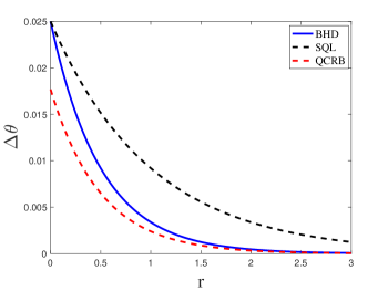
Figure 3: The effect on the phase sensitivity with the increase in the squeezing parameter $r$. Plotted with $\theta=0$, $l=1$ and $|\alpha|=20$.

Next, we show the effect of the increase in the squeezing parameter $r$ of PAs on the sensitivity of angular displacement. In Fig. 3, we see that with increase in $r$, the sensitivity of our scheme improves. And the sensitivity always goes below the SQL. With higher $r$, the sensitivity of our scheme keeps increasing and approaches the QCRB.

Due to the amplification process, the phase-sensing photon number is the total number of photons inside the interferometer, not the input photon number as the traditional MZI, that is

$$N_{Tot}=(\cosh r+\sinh r)^{2}|\alpha|^{2}+2\sinh^{2}r.$$ (30)

Eq.(29) can be written in terms of the internal number of photons, such that

$$\Delta\theta_{optimal}=\sqrt{\frac{(\cosh r-\sinh r)^{2}}{4l^{2}(N_{Tot}-2\sinh^{2}r)}}\approx\sqrt{\frac{1}{4l^{2}N_{Tot}(\cosh r+\sinh r)^{2}}}\approx\frac{1}{4l\cosh r}\sqrt{\frac{1}{N_{Tot}}}.$$ (31)

The angular displacement sensitivity can be enhanced by a factor of $2\cosh r$ compared with the SQL $(1/2l\sqrt{N})$ under the condition of $N_{Tot}\gg\sinh^{2}r$ and $\cosh r\gg 1$. When $\sinh r\gg 1$ and $\sinh^{2}r=N_{Tot}/4$, the optimal sensitivity of the scheme can reach the Heisenberg limit, approximately as $1/2lN$.

Additionally, we investigate the effect of photon losses on sensitivity. Losses can be modeled by adding fictitious beam splitters, as shown in Fig. 4. Considering two arms of the interferometer have the same transmission rates $\eta$, the optical fields $\hat{a}_{2}$ and $\hat{b}_{3}$ suffering from photon losses are given by

$$\hat{a}_{2}^{{}^{\prime}}=\sqrt{\eta}\hat{a}_{2}+\sqrt{1-\eta}\hat{v}_{1},\hat{b}_{3}^{{}^{\prime}}=\sqrt{\eta}\hat{b}_{3}+\sqrt{1-\eta}\hat{v}_{2},$$ (32)

where $\hat{v}_{1}$ and $\hat{v}_{2}$ represent vacuum.

Then, the full input-output relation is described as

$$\hat{b}_{4}^{{}^{\prime}} =\sqrt{\eta}[(e^{2il\theta}+1)(\cosh r\hat{b}_{0}+\sinh r\hat{b}_{0}^{\dagger})+(e^{2il\theta}-1)(\cosh r\hat{a}_{0}+\sinh r\hat{a}_{0}^{\dagger})]/2$$

$$+\sqrt{1-\eta}(\hat{v}_{2}-\hat{v}_{1})/\sqrt{2}.$$ (33)

After taking into account the photon losses, the sensitivity is given by

$$\Delta\theta^{{}^{\prime}}=\frac{\sqrt{-\eta\cosh r\sinh r[\cos(4l\theta)+1]+\eta\cosh(2r)+1-\eta}}{2\sqrt{\eta}l(\cosh r+\sinh r)|\alpha\cos(2l\theta)|}.$$ (34)

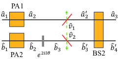
Figure 4: A lossy interferometer model, the photon losses are modeled by adding fictitious beam splitters.

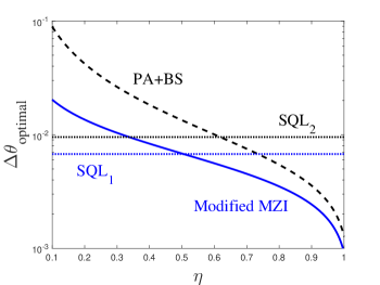
Figure 5: The optimal sensitivity versus photon losses coefficient $\eta$, where $l=1$, $r=2$ and $|\alpha|=10$. The solid line and dashed line represent the sensitivity of our scheme and PA+BS scheme, respectively. SQL₁ and SQL₂ correspond to respective standard quantum limit.

In Ref.[40], the author calculated the sensitivity of homodyne detection with photon losses in PA+BS scheme, it can resist $38\%$ photon losses in the case of $r=2$, $l=1$, and $|\alpha|=10$. Here, a comparison between our scheme and PA+BS scheme is provided under the same condition. As shown in Fig. 5, we plot the optimal sensitivity as a function of photon losses coefficient. The solid line and dashed line represent the sensitivity of our scheme and PA+BS scheme, respectively. SQL₁ and SQL₂ correspond to respective standard quantum limit. Our scheme is robust against photon losses, it can tolerate approximately photon losses of $50\%$. Besides, it should be noted that the sensitivity curve is always below PA+BS scheme, which is due to the amplification of the internal photon number.

Table 1: The sensitivities of angular displacement for different interferometer configurations with coherent state $\otimes$ vacuum state input and balanced homodyne detection

Interferometer configurations	Sensitivities of angular displacement
standard MZI	$1/2lN_{\alpha}^{1/2}$
PA+PA scheme	$1/2l\mathcal{N}N_{\alpha}^{1/2}$
PA+BS scheme	$1/[2\sqrt{2}l(N_{r}/2+\mathcal{N}/2+1)N_{\alpha}^{1/2}]$[40]
modified MZI	$1/[2l(N_{r}+\mathcal{N}+1)N_{\alpha}^{1/2}]$

In Table 1, we summarize the sensitivities of angular displacement for different interferometer configurations with coherent state $\otimes$ vacuum state input and balanced homodyne detection. The sensitivity of the PA+PA scheme is higher than that of the standard MZI by a factor of $\mathcal{N}$, where $\mathcal{N}=[(N_{r}+2)N_{r}]^{1/2}$, and $N_{\alpha}=|\alpha|^{2}$ is the mean photon number of input coherent state, $N_{r}=2\sinh^{2}r$ is the spontaneous photon number emitted from the PA. When $\sinh r\gg 1$, the sensitivity of PA+BS scheme is greater than the PA+PA scheme by a factor of $\sqrt{2}$[40]. The sensitivity of angular displacement in our scheme is further improved by a factor of $2$ compared to the PA+PA scheme, and the enhancement factor results from both effects of amplified internal photon number and squeezed noise.

4 Conclusion

In conclusion, we have investigated the estimation of angular displacements based on a modified MZI. When the unknown angular displacements are in both arms, the sensitivity using intensity detection can saturate the QCRB of angular displacements difference obtained by using the method of QFIM. For the angular displacement is only in one arm, the sensitivity using the method of homodune detection can be enhanced by a factor of $2\cosh r$ compared with the SQL and approach the QCRB. Additionally, our sheme can tolerate approximately $50\%$ photon losses. We summarize the sensitivities of angular displacement for different interferometer configurations, the sensitivity of angular displacement in our scheme is improved due to the reduction of shot noise and amplification of photon number inside the interferometer. It will have potential applications in quantum sensing and precision measurements.

Funding

This work is supported by the National Natural Science Foundation of China (Grant Nos. 11974111, 11874152, 11604069, 91536114, 11654005, and 11234003, 11474095), the Fundamental Research Funds for the Central Universities, the Science Foundation of Shanghai, China (Grant No. 17ZR1442800), and the National Key Research and Development Program of China (Grant No. 2016YFA0302001).

Disclosures

The authors declare no conflicts of interest.

References

- [1] M. J. Holland and K. Burnett, “Interferometric detection of optical phase shifts at the Heisenberg limit," Phys. Rev. Lett. 71(9), 1355-1358 (1993).
- [2] V. Giovannetti, S. Lloyd, and L. Maccone, “Quantum metrology," Phys. Rev. Lett. 96(1), 010401 (2006).
- [3] B. L. Higgins, D. W. Berry, S. D. Bartlett, H. M. Wiseman, and G. J. Pryde, “Entanglement-free heisenberg-limited phase estimation," Nature 450(7168), 393-396 (2007).
- [4] N. Thomas-Peter, B. J. Smith, A. Datta, L. Zhang, U. Dorner, and I. A. Walmsley, “Real-World Quantum Sensors: Evaluating Resources for Precision Measurement," Phys. Rev. Lett. 107(11), 113603 (2011).
- [5] H. Yonezawa, D. Nakane, T. A. Wheatley, K. Iwasawa, S. Takeda, H. Arao, K. Ohki, K. Tsumura, D. W. Berry, T. C. Ralph, H. M. Wiseman, E. H. Huntington, and A. Furusawa, “Quantum-Enhanced Optical-Phase Tracking," Science 337(6101), 1514-1517 (2012).
- [6] B. Yurke, S. L. McCall, and J. R. Klauder, “SU(2) and SU(1, 1) interferometers," Phys. Rev. A 33(6), 4033-4054 (1986).
- [7] W. N. Plick, J. P. Dowling, and G. S. Agarwal, “Coherent-light-boosted, sub-shot noise, quantum interferometry," New J. Phys. 12(8), 083014 (2010).
- [8] Z. Y. Ou, “Enhancement of the phase-measurement sensitivity beyond the standard quantum limit by a nonlinear interferometer," Phys. Rev. A 85(2), 023815 (2012).
- [9] A. M. Marino, N. V. Corzo Trejo, and P. D. Lett, “Effect of losses on the performance of an SU(1,1) interferometer," Phys. Rev. A 86(2), 023844 (2012).
- [10] D. Li, C.-H. Yuan, Z. Y. Ou, and W. Zhang, “The phase sensitivity of an SU (1, 1) interferometer with coherent and squeezed-vacuum light," New J. Phys. 16(7), 073020 (2014).
- [11] M. Gabbrielli, L. Pezzè, and A. Smerzi, “Spin-Mixing Interferometry with Bose-Einstein Condensates," Phys. Rev. Lett. 115(16), 163002 (2015).
- [12] Z.-D. Chen, C.-H. Yuan, H.-M. Ma, D. Li, L. Q. Chen, Z. Y. Ou, and W. Zhang, “Effects of losses in the atom-light hybrid SU(1,1) interferometer," Opt. Express 24(16), 17766-17778 (2016).
- [13] C. Sparaciari, S. Olivares, and M. G. A. Paris, “Gaussian-state interferometry with passive and active elements," Phys. Rev. A 93(2), 023810 (2016).
- [14] D. Li, B. T. Gard, Y. Gao, C.-H. Yuan, W. Zhang, H. Lee, and J. P. Dowling, “Phase sensitivity at the Heisenberg limit in an SU(1,1) interferometer via parity detection," Phys. Rev. A 94(6), 063840 (2016).
- [15] Q.-K. Gong, X.-L. Hu, D. Li, C.-H. Yuan, Z. Y. Ou, and W. Zhang, “Intramode correlations enhanced phase sensitivities in an SU(1,1) interferometer," Physical Review A 96(3), 033809 (2017).
- [16] E. Giese, S. Lemieux, M. Manceau, R. Fickler, and R.W. Boyd, “Phase sensitivity of gain-unbalanced nonlinear interferometers," Phys. Rev. A 96(5), 053863 (2017).
- [17] X.-L. Hu, D. Li, L. Q. Chen, K. Zhang, W. Zhang, and C.-H. Yuan, “Phase estimation for an SU(1,1) interferometer in the presence of phase diffusion and photon losses," Phys. Rev. A 98(2), 023803 (2018).
- [18] J. Jing, C. Liu, Z. Zhou, Z. Y. Ou, and W. Zhang, “Realization of a nonlinear interferometer with parametric amplifiers," Appl. Phys. Lett. 99(1), 011110 (2011).
- [19] F. Hudelist, J. Kong, C. Liu, J. Jing, Z. Y. Ou, and W. Zhang, “Quantum metrology with parametric amplifier-based photon correlation interferometers," Nat. Commun. 5(1), 3049 (2014).
- [20] B. Chen, C. Qiu, S. Chen, J. Guo, L. Q. Chen, Z. Y. Ou, and W. Zhang, “Atom-Light Hybrid Interferometer," Phys. Rev. Lett. 115(4), 043602 (2015).
- [21] C. Qiu, S. Chen, L. Q. Chen, B. Chen, J. Guo, Z. Y. Ou, and W. Zhang, “Atom–light superposition oscillation and Ramsey-like atom–light interferometer," Optica 3(7), 775-780 (2016).
- [22] D. Linnemann, H. Strobel, W. Muessel, J. Schulz, R. J. Lewis-Swan, K. V. Kheruntsyan, and M. K. Oberthaler, “Quantum-Enhanced Sensing Based on Time Reversal of Nonlinear Dynamics," Phys. Rev. Lett. 117(1), 013001 (2016).
- [23] S. Lemieux, M. Manceau, P. R. Sharapova, O. V. Tikhonova, R. W. Boyd, G. Leuchs, and M. V. Chekhova, “Engineering the Frequency Spectrum of Bright Squeezed Vacuum via Group Velocity Dispersion in an SU(1,1) Interferometer," Phys. Rev. Lett. 117(18), 183601 (2016).
- [24] M. Manceau, G. Leuchs, F. Khalili, and M. Chekhova, “Detection Loss Tolerant Supersensitive Phase Measurement with an SU(1,1) Interferometer," Phys. Rev. Lett. 119(22), 223604 (2017).
- [25] P. Gupta, B. L. Schmittberger, B. E. Anderson, K. M. Jones, and P. D. Lett, “Optimized phase sensing in a truncated SU(1,1) interferometer," Opt. Express 26(1), 391-401 (2018).
- [26] W. Du, J. Jia, J. F. Chen, Z. Y. Ou, and W. Zhang, “Absolute sensitivity of phase measurement in an SU(1,1) type interferometer," Opt. Lett. 43(5), 1051-1054 (2018).
- [27] J. Kong, Z. Y. Ou, and W. Zhang, “Phase-measurement sensitivity beyond the standard quantum limit in an interferometer consisting of a parametric amplifier and a beam splitter," Phys. Rev. A 87(2), 023825 (2013).
- [28] S. S. Szigeti, R. J. Lewis-Swan, and S. A. Haine, “Pumped-Up SU(1,1) Interferometry," Phys. Rev. Lett. 118(15), 150401 (2017).
- [29] B. E. Anderson, P. Gupta, B. L. Schmittberger, T. Horrom, C. Hermann-Avigliano, K. M. Jones, and P. D. Lett, “Phase sensing beyond the standard quantum limit with a variation on the SU (1, 1) interferometer," Optica 4(7), 752-756 (2017).
- [30] W. Du, J. Kong, J. Jia, S. Ming, C. H. Yuan, J. F. Chen, Z. Y. Ou, M. W. Mitchell, and W. Zhang, “SU(2)-in-SU(1,1) nested interferometer," arXiv:2004.14266
- [31] X. Zuo, Z. Yan, Y. Feng, J. Ma, X. Jia, C. Xie, and K. Peng, “Quantum Interferometer Combining Squeezing and Parametric Amplification," Phys. Rev. Lett. 124(17), 173602 (2020).
- [32] M. Padgett and R. Bowman, “Tweezers with a twist," Nat. Photonics 5(6), 343-348 (2011).
- [33] M. P. J. Lavery, F. C. Speirits, S. M. Barnett, and M. J. Padgett, “Detection of a Spinning Object Using Light’s Orbital Angular Momentum," Science 341(6145), 537-540 (2013).
- [34] J. Courtial, D. A. Robertson, K. Dholakia, L. Allen, and M. J. Padgett, “Rotational Frequency Shift of a Light Beam," Phys. Rev. Lett. 81(22), 4828-4830 (1998).
- [35] N. Uribe-Patarroyo, A. Fraine, D. S. Simon, O. Minaeva, and A. V. Sergienko, “Object Identification Using Correlated Orbital Angular Momentum States," Phys. Rev. Lett. 110(4), 043601 (2013).
- [36] O. S. Magaña-Loaiza, M. Mirhosseini, B. Rodenburg, and R. W. Boyd, “Amplification of Angular Rotations Using Weak Measurements," Phys. Rev. Lett. 112(20), 200401 (2014).
- [37] V. D’Ambrosio, N. Spagnolo, L. Del Re, S. Slussarenko, Y. Li, L. C. Kwek, L. Marrucci, S. P. Walborn, L. Aolita, and F. Sciarrino, “Photonic polarization gears for ultra-sensitive angular measurements." Nat. Commun. 4(1), 2432 (2013).
- [38] A. K. Jha, G. S. Agarwal, and R. W. Boyd, “Supersensitive measurement of angular displacements using entangled photons," Phys. Rev. A 83(5), 053829 (2011).
- [39] J. Liu, W. Liu, S. Li, D. Wei, H. Gao, and F. Li, “Enhancement of the angular rotation measurement sensitivity based on SU(2) and SU(1, 1) interferometers," Photonics Res. 5(6), 617-622 (2017).
- [40] J.-D. Zhang, C.-F. Jin, Z.-J. Zhang, L.-Z. Cen, J.-Y. Hu, and Y. Zhao, “Super-sensitive angular displacement estimation via an su(1,1)-su(2) hybrid interferometer," Opt. Express 26(25), 33080-33090 (2018).
- [41] J.-D. Zhang, Z.-J. Zhang, L.-Z. Cen, C. You, S. Adhikari, J. P. Dowling, and Y. Zhao, “Orbital-angular-momentum-enhanced estimation of sub-Heisenberg-limited angular displacement with two-mode squeezed vacuum and parity detection," Opt. Express 26(13), 16524-16534 (2018).
- [42] J.-D. Zhang, Z.-J. Zhang, L.-Z. Cen, J.-Y Hu, and Y. Zhao, “Tried-and-true binary strategy for angular displacement estimation based upon fidelity appraisal," Opt. Express 27(4), 5512-5522 (2019).
- [43] J.-D. Zhang, Z.-J. Zhang, L.-Z. Cen, J.-Y Hu, and Y. Zhao, “Super-resolved angular displacement estimation based upon a Sagnac interferometer and parity measurement," Opt. Express 28(3), 4320-4332 (2020).
- [44] C. W. Helstrom, Quantum Detection and Estimation Theory (Academic, 1976).
- [45] A. S. Holevo, Probabilistic and Statistical Aspects of Quantum Theory (Springer Science and Bussiness Media, 2011).
- [46] S. L. Braunstein and C. M. Caves, “Statistical distance and the geometry of quantum states," Phys. Rev. Lett. 72(22), 3439-3443 (1994).