TUM-HEP-1280/20

$B_{d,s}\to\gamma\ell\bar{\ell}$ decay with an energetic photon

Martin Beneke^a, Christoph Bobeth^a and Yu-Ming Wang^b

^aPhysik Department T31,
James-Franck-Straße 1, Technische Universität München,
D–85748 Garching, Germany

^bSchool of Physics, Nankai University,
Weijin Road 94, 300071 Tianjin, China

We calculate the differential branching fraction, lepton forward-backward asymmetry and direct CP asymmetry for $B_{d,s}\to\gamma\ell\bar{\ell}$ decays with an energetic photon. We employ factorization methods, which result in rigorous next-to-leading order predictions in the strong coupling at leading power in the large-energy/heavy-quark expansion, together with estimates of power corrections and a resonance parameterization of sub-leading power form factors in the region of small lepton invariant mass $q^{2}$. The $B_{d,s}\to\gamma\ell\bar{\ell}$ decay shares features of the charged-current decay $B_{u}\to\gamma\ell\bar{\nu}_{\ell}$, and the FCNC decays $B\to K^{(*)}\ell\bar{\ell}$. As in the former, the leading-power decay rates can be expressed in terms of the $B$-meson light-cone distribution amplitude and short-distance factors. However, similar to $B\to K^{(*)}\ell\bar{\ell}$, four-quark and dipole operators contribute to the $B_{d,s}\to\gamma\ell\bar{\ell}$ decay in an essential way, limiting the calculation to $q^{2}\lesssim 6$ GeV² below the charmonium resonances in the lepton invariant mass spectrum. A detailed analysis of the main observables and theoretical uncertainties is presented.

1 Introduction

The semileptonic flavour-changing neutral-current (FCNC) decays driven by the quark-level transitions $b\to q\,\ell\bar{\ell}$ with $q=d,s$ and $\ell=e,\mu,\tau$ are important tests of the dynamics of the quark and lepton sectors in the framework of the standard model (SM) and constitute very sensitive probes of nonstandard effects.

The exclusive $B\to K^{(*)}\ell\bar{\ell}$ decays are experimentally most easily accessible due to their comparatively sizeable branching fractions of $\mathcal{O}(10^{-6})$. The angular distributions of their three- and four-body final states are among the prime targets of LHCb and Belle II for $\ell=e,\mu$, because they offer many CP-symmetric and CP-asymmetric observables. However, the hadronic nonperturbative effects entering the theoretical treatment are complex ranging from form factors to resonant contributions, preventing currently theoretical calculations with percent accuracy. In contrast, the purely leptonic decays $B_{q}\to\ell\bar{\ell}$ allow theoretical control of hadronic effects at the percent level [1], because they depend—apart from higher-order QED corrections [2, 3]— only on the $B$-meson decay constant, which can be computed in QCD lattice calculations with sub-percent accuracy [4]. On the other hand the helicity suppression of the two-body final state leads to tiny branching fractions of $\mathcal{O}(10^{-9})$ for $\ell=\mu$, requiring huge data samples at LHC in order to perform measurements with precision comparable to the prediction. Nevertheless this decay has been observed by LHCb [5], CMS [6] and ATLAS [7] with a rate compatible with SM predictions.

Compared to the strong research activities on the aforementioned decay modes, the radiative leptonic decays $B_{q}\to\gamma\ell\bar{\ell}$ have received relatively little attention. The additional photon in the final state implies suppression by the electromagnetic coupling, but lifts the very different helicity suppression for $\ell=e$ and $\ell=\mu$ present in $B_{q}\to\ell\bar{\ell}$. The decay rates of $B_{q}\to\gamma\ell\bar{\ell}$ become comparable for the electron and muon final states and can be almost $\mathcal{O}(10^{-8})$ for $q=s$ [8, 9, 10, 11]. Further, the angular distribution offers complementary observables to test the short-distance couplings. So far there are no experimental studies of the $B_{q}\to\gamma\ell\bar{\ell}$ decays, which for small photon energies also constitute a background process in the experimental analyses of $B_{q}\to\ell\bar{\ell}$ in the dilepton-invariant mass side-band [12, 5, 13].

Besides testing the SM, the theoretical interest in $B_{q}\to\gamma\ell\bar{\ell}$ also derives from the structure of hadronic effects. The limit of large photon energy $E_{\gamma}\gg\Lambda_{\text{QCD}}$, where $\Lambda_{\text{QCD}}$ denotes the strong interaction scale, allows for a systematic treatment of nonperturbative effects when adopting the framework of QCD factorization and soft-collinear effective theory (SCET). As pointed out in [14], in this limit the leading nonperturbative corrections become universal for the decays $B_{u}\to\gamma\ell\bar{\nu}_{\ell}$, $B_{q}\to\gamma\gamma$ and $B_{q}\to\gamma\ell\bar{\ell}$, relating thus hadronic effects in $b\to u\ell\bar{\nu}_{\ell}$, $b\to q\gamma$ and $b\to q\ell\bar{\ell}$, respectively, and offering a programme for the combined analysis of long- and short-distance quantities in these decays. Other approaches are available in the literature relying on the $B_{q}\to\gamma$ form factor calculation with dispersive methods and quark models [8, 9, 11, 15]. The case of very soft photons due to initial-state radiation has been considered in the framework of heavy-hadron chiral perturbation theory in [12].

The factorization programme has been carried out for $B_{u}\to\gamma\ell\bar{\nu}_{\ell}$ starting within QCD factorization (QCDF) [16, 17] and has then been extended to the two-step matching in SCET [18, 19] at leading power (LP) in $\Lambda_{\text{QCD}}/m_{b}$, including next-to-leading order (NLO) radiative QCD corrections and resummation of the associated large logarithms. Next-to-leading power (NLP) corrections at lowest order in QCD have been considered in [20], studying the consequences for the form factor symmetry relation. The NLP corrections have been scrutinized further with sum rule calculations [21, 22, 23, 24].

The decay $B_{q}\to\gamma\ell\bar{\ell}$ appears as a hybrid of the charged-current decay $B_{u}\to\gamma\ell\bar{\nu}_{\ell}$, which is driven by tree-level electroweak $b\to u\ell\bar{\nu}_{\ell}$ transitions and the FCNC decays $B\to K^{(*)}\ell\bar{\ell}$, which receive contributions from semileptonic $b\to s+(\gamma,\,\ell\bar{\ell})$ as well as from hadronic $b\to s+(g,\,q\bar{q})$ transitions. When the final-state photon carries large energy relative to the strong interaction scale, the non-hadronic final state of the $B_{q}\to\gamma\ell\bar{\ell}$ decay enables the calculation of the relevant form factors in terms of the $B$-meson light-cone distribution amplitude (LCDA) at LP in an expansion in the energy of the photon, similar to the decay $B_{u}\to\gamma\ell\bar{\nu}_{\ell}$ [18, 19]. On the other hand, the contribution of $b\to sq\bar{q}$ four-quark operators to $B_{q}\to\gamma\ell\bar{\ell}$ introduces issues familiar from $B\to K^{(*)}\ell\bar{\ell}$ decay, such as the presence of charmonium resonances in the $\ell\bar{\ell}$ invariant mass spectrum that limit the applicability of factorization methods to this decay [25, 26].

Previous work on $B_{q}\to\gamma\ell\bar{\ell}$ [8, 9, 27, 10, 11] has usually focused on providing theoretical calculations of the (differential) decay rate in the entire kinematically allowed regions in terms of $B\to\gamma^{*}$ form factors. This approach inevitably requires some amount of theoretical modelling of the form factors, and neglects “non-factorizable” $\mathcal{O}(\alpha_{s})$ corrections from the $b\to sq\bar{q}$ four-quark and chromomagnetic dipole operators, which are known to be sizeable for $B\to K^{(*)}\ell\bar{\ell}$ decays [25].

In contrast, our focus is on the kinematically more restricted region of photon energy $E_{\gamma}\gg\Lambda_{\text{QCD}}$, while making maximal use of factorization methods applicable in this limit. We perform a SCET analysis of $B_{q}\to\gamma\ell\bar{\ell}$ including $\mathcal{O}(\alpha_{s})$ QCD corrections at LP. We further include local NLP corrections in $\mathcal{O}(\alpha_{s}^{0})$ explicitly, whereas non-local NLP contributions are parametrized following [20, 22]. The analysis is more involved for the FCNC $b\to q\ell\bar{\ell}$ transitions compared to the tree-level decay $b\to u\ell\bar{\nu}_{\ell}$ due to the extended weak operator basis (2.1). Parts of our analysis are related to earlier works on $B_{u}\to\gamma\ell\bar{\nu}_{\ell}$, $B_{q}\to\gamma\gamma$ and $B\to K^{(*)}\ell\bar{\ell}$ within QCDF [25, 14, 28] or SCET [18, 19, 20, 22]. The factorization approach then allows us to express the decay amplitudes in terms of only the $B$-meson light-cone distribution amplitude (LCDA) at LP in the heavy-quark/large-energy expansion. The modelling of form factors is necessary only at sub-leading power in this expansion. The result is expected to be valid for sufficiently broad bins in invariant mass $q^{2}$ of the lepton pair below the charmonium resonances, $q^{2}\lesssim 6\,\text{GeV}^{2}$, and above the narrow light-meson resonances. The latter restriction arises, since estimates following [29] imply that global duality is violated not only by charmonium, but also by the light-meson resonances. In order to extend our calculations to observables local in $q^{2}$, we incorporate the light-meson resonances in our model for the sub-leading power form factors, which confirms the estimates of duality violation. This together with numerical cancellations of various otherwise dominant leading-power effects leads us to conclude that theoretical predictions of $B_{q}\to\gamma\ell\bar{\ell}$ observables in the low-$q^{2}$ region are plagued by large theoretical uncertainties.

The outline of the paper is as follows. In Section 2 we detail the conventions for the effective weak interaction Lagrangian and parametrize the $B_{q}\to\gamma\ell\bar{\ell}$ amplitude in terms of hadronic tensors and the associated form factors. We employ a mix of QCD factorization and SCET techniques to calculate in Section 3 the hadronic tensors at LP including $\mathcal{O}(\alpha_{s})$ radiative corrections and the summation of logarithms, and at NLP in $\mathcal{O}(\alpha_{s}^{0})$. We next discuss issues related to the interpretation of the rescattering phase from factorization, duality violation and resonances. We then parametrize the single NLP form factor, which cannot be computed in factorization, and discuss the model that will be used for the numerical analysis. Section 4 is devoted to a detailed discussion of the various contributions to the $B_{q}\to\gamma\ell\bar{\ell}$ decay amplitude, which exhibits sizeable corrections and cancellations in the $q^{2}$ region of interest. We show the differential branching fraction, lepton forward-backward asymmetry and direct CP asymmetry as functions of $q^{2}$ and integrated in various bins. We conclude in Section 5. Further details on definitions, conventions, final-state radiation and the $B$-meson LCDA are given in Appendices.

2 $B_{q}\to\gamma\ell\bar{\ell}$ amplitude

2.1 $\Delta B=1$ effective theory

The low-energy effective theory of electroweak interactions in the SM for ${\Delta B}=1$ semileptonic $b\to q\ell\bar{\ell}$ ($q=d,s$) decays is

$$\mathcal{L}_{\text{eff}} =\mathcal{N}_{\text{ew}}\left[\sum_{i=1}^{6}C_{i}\,P_{i}^{(c)}+\frac{\alpha_{\text{em}}}{4\pi}\sum_{i=7}^{10}C_{i}\,P_{i}+\frac{\lambda_{u}^{(q)}}{\lambda_{t}^{(q)}}\sum_{i=1}^{2}C_{i}\left(P^{c}_{i}-P^{u}_{i}\right)\right]+\text{h.c.}\,.$$ (2.1)

We adopt the basis proposed in [30, 31] for the operators $P_{i}$. The normalization factor $\mathcal{N}_{\text{ew}}\equiv 2\sqrt{2}\,G_{F}\,\lambda_{t}^{(q)}$ contains products of elements of the quark mixing matrix $\lambda_{U}^{(q)}\equiv V_{Ub}V_{Uq}^{*}$ for $U=u,c,t$. The term proportional to $\lambda_{u}^{(q)}$ leads to tiny doubly Cabibbo-suppressed CP-asymmetries in $b\to s$ transitions, but is not negligible in $b\to d$ transitions. The Wilson coefficients $C_{i}(\nu)$ are evaluated at the hard scale $\nu$ of the order of the $b$-quark mass $m_{b}$, after renormalization group (RG) evolution [32, 33] from the electroweak scale. There are four-quark operators, the so-called charged-current operators $P_{1,2}^{c,u}$ and the QCD-penguin operators $P_{3,4,5,6}$. The remaining operators in the SM are the semileptonic operators

$$P_{9} =[\bar{q}\gamma^{\mu}P_{L}b][\bar{\ell}\gamma_{\mu}\ell], P_{10} =[\bar{q}\gamma^{\mu}P_{L}b][\bar{\ell}\gamma_{\mu}\gamma_{5}\ell],$$ (2.2)

with $$P_{L/R}=(1\mp\gamma_{5})/2$$ and the dipole operators

$$P_{7} =-\frac{{\overline{m}}_{b}}{e}\big{[}\bar{q}\sigma^{\mu\nu}P_{R}b\big{]}F_{\mu\nu}, P_{8} =-\frac{g_{s}{\overline{m}}_{b}}{e^{2}}\big{[}\bar{q}\sigma^{\mu\nu}P_{R}T^{a}b\big{]}G^{a}_{\mu\nu},$$ (2.3)

where ${\overline{m}}_{b}$ is the running $b$-quark mass in the ${\overline{\text{MS}}}$ scheme at the scale $\nu$. The QED$\,\times\,$QCD covariant derivative is chosen as $D_{\mu}\psi\equiv(\partial_{\mu}-ieQ_{\psi}A_{\mu}-ig_{s}T^{a}G^{a}_{\mu})\psi$, following [25], and $Q_{\ell}=-1$ for leptons, $Q_{u}=+2/3$, $Q_{d}=-1/3$ for quarks.

2.2 $B_{q}\to\gamma\ell\bar{\ell}$ form factors

The transition amplitude for the decay of the ${\overline{B}}_{q}$ meson is

$${\overline{\mathcal{A}}}\equiv{\overline{\mathcal{A}}}({\overline{B}}_{q}\to\gamma\ell\bar{\ell}) =\big{\langle}{\gamma(k,\epsilon)\,\ell(p_{\ell})\,{\overline{\ell}}(p_{\overline{\ell}})}\big{|}\mathcal{L}_{\text{eff}}\big{|}{{\overline{B}}_{q}(p)}\big{\rangle},$$ (2.4)

where $\epsilon$ is the polarization vector of the photon, and $k$ its momentum, related to the dilepton momentum $q\equiv p_{\ell}+p_{\overline{\ell}}=p-k$. When working to lowest non-vanishing order in the electromagnetic coupling $\alpha_{\text{em}}=e^{2}/(4\pi)$, but to all orders in QCD, the amplitude can be written in the form

$${\overline{\mathcal{A}}}=\, ie\,\frac{\alpha_{\text{em}}}{4\pi}\,\mathcal{N}_{\text{ew}}\,\epsilon^{\star}_{\mu}\Bigg{\{}\sum_{i=1}^{9}\eta_{i}C_{i}\left[T^{\mu\nu}_{i}\,\big{\langle}{\ell{\overline{\ell}}}\big{|}{\overline{\ell}}\gamma_{\nu}\ell\big{|}{0}\big{\rangle}+S_{\nu}^{(i)}\int d^{4}x\,e^{ikx}\,\big{\langle}{\ell{\overline{\ell}}}\big{|}\text{T}\{j_{\ell}^{\mu}(x),[{\overline{\ell}}\gamma^{\nu}\ell](0)\}\big{|}{0}\big{\rangle}\right]$$

$$+\,C_{10}\left[T^{\mu\nu}_{10}\,\big{\langle}{\ell{\overline{\ell}}}\big{|}{\overline{\ell}}\gamma_{\nu}\gamma_{5}\ell\big{|}{0}\big{\rangle}+S_{\nu}^{(10)}\int d^{4}x\,e^{ikx}\,\big{\langle}{\ell{\overline{\ell}}}\big{|}\text{T}\{j_{\ell}^{\mu}(x),[{\overline{\ell}}\gamma^{\nu}\gamma_{5}\ell](0)\}\big{|}{0}\big{\rangle}\right]\Bigg{\}}$$

$$=\, ie\,\frac{\alpha_{\text{em}}}{4\pi}\,\mathcal{N}_{\text{ew}}\,\epsilon^{\star}_{\mu}\left\{\sum_{i=1}^{9}\eta_{i}C_{i}\left[T^{\mu\nu}_{i}L_{V,\nu}+L_{V}^{\mu\nu}S_{\nu}^{(i)}\right]+C_{10}\left[T^{\mu\nu}_{10}L_{A,\nu}+L_{A}^{\mu\nu}S_{\nu}^{(10)}\right]\right\}\,,$$ (2.5)

where $j_{\ell}^{\mu}=Q_{\ell}\,{\overline{\ell}}\gamma^{\mu}\ell$ denotes the leptonic electromagnetic current. The quantities $T^{\mu\nu}_{i}$ and $S_{\nu}^{(i)}$ define hadronic matrix elements, which encode all QCD effects at lowest non-vanishing order in the electromagnetic interaction. The calculation of these hadronic tensors is one of the main purposes of this work.

We briefly consider the terms involving $S_{\nu}^{(i)}$. The structure of the purely leptonic tensor multiplying these terms shows that they correspond to final-state radiation (FSR) of the photon from the lepton-pair. The hadronic matrix elements $S_{\nu}^{(i)}$ are $B$-meson to vacuum matrix elements, which must be proportional to the $B$-meson momentum $p_{\nu}$. The contraction of the vectorial leptonic tensor with $p_{\nu}$ vanishes, $p_{\nu}L_{V}^{\mu\nu}=0$, while the corresponding contraction of the axi-vectorial leptonic tensor is proportional to the lepton mass. The only non-vanishing FSR contribution is therefore due to $P_{10}$ [34] and helicity-suppressed. The QCD effects are entirely described by the $B$-meson decay constant, since

$$S_{\nu}^{(10)} =\big{\langle}{0}\big{|}\bar{q}\,\gamma_{\nu}P_{L}\,b\big{|}{{\overline{B}}_{q}(p)}\big{\rangle}\equiv-\frac{i}{2}f_{B_{q}}p_{\nu}.$$ (2.6)

The FSR contribution is tiny except in very small phase-space regions, and can be safely neglected in the later numerical analysis. For further details on the FSR contribution we refer to Appendix B.

Our main concern are therefore the hadronic tensors $T^{\mu\nu}_{i}$, sometimes referred to as structure-dependent (SD) contributions. The individual SD contributions of each operator are contracted with the vector or axial-vector lepton currents

$$L_{V(A)}^{\alpha} =\big{\langle}{\ell{\overline{\ell}}}\big{|}{\overline{\ell}}\gamma^{\alpha}(\gamma_{5})\ell\big{|}{0}\big{\rangle}={\overline{u}}(p_{\ell})\,\gamma^{\alpha}(\gamma_{5})\,v(p_{{\overline{\ell}}})\,, \eta_{i} =\left\{\begin{array}[]{ll}1&\quad i=9,10\\ Q_{\ell}&\quad i\neq 9,10\end{array}\right..$$ (2.9)

The hadronic tensors $T_{i}^{\mu\nu}(k,q)$ are the correlation functions

$$T_{i}^{\mu\nu} =\int\!d^{4}x\,e^{ikx}\,\big{\langle}{0}\big{|}\text{T}\{j^{\mu}_{f}(x),\,[\bar{q}\,\gamma^{\nu}P_{L}\,b](0)\}\big{|}{{\overline{B}}_{q}}\big{\rangle}, i =9,10,$$ (2.10)

$$T_{7A}^{\mu\nu} =\frac{2{\overline{m}}_{b}}{q^{2}}\int\!d^{4}x\,e^{ikx}\,\big{\langle}{0}\big{|}\text{T}\{j^{\mu}_{f}(x),\,[\bar{q}\,i\sigma^{\nu\alpha}q_{\alpha}P_{R}\,b](0)\}\big{|}{{\overline{B}}_{q}}\big{\rangle},$$ (2.11)

$$T_{7B}^{\mu\nu} =\frac{2{\overline{m}}_{b}}{q^{2}}\int\!d^{4}x\,e^{iqx}\,\big{\langle}{0}\big{|}\text{T}\{j^{\nu}_{f}(x),\,[\bar{q}\,i\sigma^{\mu\alpha}k_{\alpha}P_{R}\,b](0)\}\big{|}{{\overline{B}}_{q}}\big{\rangle},$$ (2.12)

$$T_{i}^{\mu\nu} =i\,\frac{(4\pi)^{2}}{q^{2}}\!\!\int\!d^{4}x\,d^{4}y\,e^{ikx}e^{iqy}\,\big{\langle}{0}\big{|}\text{T}\{j^{\mu}_{f}(x),\,j^{\nu}_{f}(y),\,P_{i}(0)\}\big{|}{{\overline{B}}_{q}}\big{\rangle}, i =1,\ldots,6,8$$ (2.13)

with the electromagnetic quark-current $j^{\mu}_{f}=\sum_{f}Q_{f}\,[\bar{f}\gamma^{\mu}f]$. Here $f$ is summed over all five active quark flavours. The hadronic tensors $T_{9,10}^{\mu\nu}$ are time-ordered products of the weak currents with the electromagnetic current in direct analogy with the charged-current decay $B_{u}\to\gamma\ell\bar{\nu}_{\ell}$. The contribution from $P_{7}$, $T_{7}^{\mu\nu}=T_{7A}^{\mu\nu}+T_{7B}^{\mu\nu}$, has been split into the part $T_{7A}^{\mu\nu}$, which accounts for the emission of the final-state photon from the constituents of the $B$-meson, and the part $T_{7B}^{\mu\nu}$, where the on-shell photon is emitted directly from $P_{7}$, while the electromagnetic current produces the virtual photon with momentum $q$, which decays into the lepton pair. Quite generally, we refer to these two different contributions as $A$- and $B$-type, respectively. Similarly, the hadronic tensors $T_{1,\ldots 6}^{\mu\nu}$ for the four-quark operators contain $A$-type and $B$-type parts, depending on which of the two electromagnetic currents is inserted into a $B$-meson constituent quark line, and a further annihilation-type contribution, where neither of the on-shell and virtual photon is emitted from the initial-state quarks. See Figure 1 for the lowest order diagrams in $\alpha_{s}$ representing these three contributions.

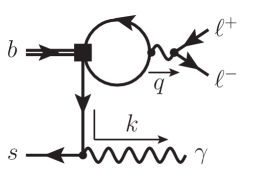
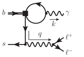
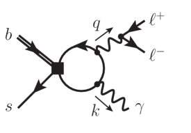
Figure 1: The three possible contractions ($A$-type left, $B$-type middle) of the four-quark operators $P_{1,\ldots,6}$ at $\mathcal{O}(\alpha_{s}^{0})$. The insertion shown on the right is power-suppressed. The $B$-type insertion is power-suppressed when $q^{2}\sim m_{b}^{2}$ but LP when $q^{2}\sim E_{\gamma}\Lambda_{\text{QCD}}$, $m_{b}\Lambda_{\text{QCD}}$. For the first two diagrams, there exists a counterpart where the real/virtual photon is attached to the heavy-quark line (double line), which, however, is power-suppressed. The external photon line with momentum $k$ symbolizes the electromagnetic current $j^{\mu}_{f}(x)$ in the definition (2.13) of the hadronic tensor $T_{i}^{\mu\nu}$, the virtual photon including its decay into the lepton-pair graphically represents the current $j^{\mu}_{f}(y)$. The ${\overline{B}}_{s}$-meson state is represented by its leading partonic constituents, a $b$-quark and a light anti-quark.

The hadronic tensors $T_{i}^{\mu\nu}(k,q)$ can be parametrized in terms of scalar form factors. Their number is determined by exploiting the Ward identities (e.g. [35]) that hold upon contraction with $k$ and $q$,

$$k_{\mu}T_{9,10}^{\mu\nu}=k_{\mu}T_{7A}^{\mu\nu}=q_{\nu}T_{7B}^{\mu\nu} =0,$$ (2.14)

$$k_{\mu}T_{i}^{\mu\nu}=q_{\nu}T_{i}^{\mu\nu} =0, \quad i =1,\ldots,6,8,$$

together with the algebraic relations $k_{\mu}T_{7B}^{\mu\nu}=q_{\nu}T_{7A}^{\mu\nu}=0$. The Ward identities and the transversality of the on-shell photon, $\epsilon^{\star}\cdot k=0$, which implies that $\mu$ is a transverse index, lead to the Lorentz decomposition

$$T_{i}^{\mu\nu}(k,q) =\frac{1}{m_{B_{q}}}\Big{[}\left[g^{\mu\nu}(k\cdot q)-q^{\mu}k^{\nu}\right]\left(F_{L}^{(i)}-F_{R}^{(i)}\right)+i\varepsilon^{\mu\nu\alpha\beta}q_{\alpha}k_{\beta}\left(F_{L}^{(i)}+F_{R}^{(i)}\right)\Big{]}$$

$$=E_{\gamma}\left[g_{\perp}^{\mu\nu}\left(F_{L}^{(i)}-F_{R}^{(i)}\right)+i\varepsilon^{\mu\nu}_{\perp}\left(F_{L}^{(i)}+F_{R}^{(i)}\right)\right],$$ (2.15)

which contains two helicity form factors $F_{L,R}^{(i)}$ for each operator $P_{i}$. We use the convention $\varepsilon_{0123}=-1$, for definitions of $g_{\perp}^{\mu\nu}$ and $\varepsilon^{\mu\nu}_{\perp}$ we refer to Appendix A.

Below we will employ QCD factorization techniques to factorize the hadronic matrix elements $T^{\mu\nu}_{i}(k,q)$ and the corresponding form factors $F_{h}^{(i)}$ $(h=L,R)$ for large photon energy $E_{\gamma}\gg\Lambda_{\text{QCD}}$. In this limit the right-helicity form factors $F_{R}^{(i)}$ are suppressed by $\Lambda_{\text{QCD}}/E_{\gamma}$ compared to $F_{L}^{(i)}$ due to the left-handedness of the weak interaction and helicity-conservation of QCD at high energy. One often defines vector $F_{V}^{(i)}=F_{L}^{(i)}+F_{R}^{(i)}$ and axial-vector $F_{A}^{(i)}=F_{L}^{(i)}-F_{R}^{(i)}$ form factors, hence the symmetry $F_{V}^{(i)}=F_{A}^{(i)}$ between the transversity form factors holds at LP in the heavy-quark/large-energy expansion.

3 Factorization of form factors

QCD factorization can be applied to the hadronic process if the on-shell photon is very energetic $E_{\gamma}\gg\Lambda_{\text{QCD}}$. It is most intuitive to work in the rest frame of the $B_{q}$ meson, where the three-vectors $\vec{k}$ and $\vec{q}$ are back-to-back and the constituent $b$ and $q$ quarks of the $B_{q}$ meson will have soft residual momenta of order $\Lambda_{\text{QCD}}$.

We introduce the four velocity $v$ ($v^{2}=1$) of the ${\overline{B}}_{q}$-meson and a pair of light-like vectors ${n_{-}}$ and ${n_{+}}$, with $n_{-}^{2}=n_{+}^{2}=0$, ${n_{-}}{n_{+}}=2$, $v=({n_{-}}+{n_{+}})/2$, such that

$$p^{\mu} =m_{B_{q}}v^{\mu}, k^{\mu} =\frac{{n_{+}}k}{2}\,n_{-}^{\mu}=\frac{m_{B_{q}}}{2}y\,n_{-}^{\mu}, q^{\mu} =\frac{m_{B_{q}}}{2}\left[n_{+}^{\mu}+\left(1-y\right)n_{-}^{\mu}\right].$$ (3.1)

The photon energy $E_{\gamma}=({n_{+}}k)/2=(m_{B_{q}}^{2}-q^{2})/(2m_{B_{q}})$. For later convenience we define $y\equiv 2E_{\gamma}/m_{B_{q}}$ with $0\leq y\leq 1-4m_{\ell}^{2}/m_{B_{q}}^{2}$. We refer to momenta $r$ with large component ${n_{+}}r=\mathcal{O}(E_{\gamma},m_{b})$ in the direction of ${n_{-}}$ and small $r^{2}$ as collinear. Anti-collinear momenta have this property with ${n_{+}}\leftrightarrow{n_{-}}$ interchanged. Hence the momentum $k^{\mu}$ of the on-shell final-state photon is collinear. The nature of the lepton-pair or virtual photon momentum $q^{\mu}$ depends on whether the real photon energy $E_{\gamma}$ is close to its maximal kinematically allowed value $m_{B_{q}}/2$, corresponding to $y=1$. Since $q^{2}/m_{B_{q}}^{2}=1-2E_{\gamma}/m_{B_{q}}=1-y$, we consider two scalings for $q^{2}$:

• anti-hard-collinear (${\overline{\text{hc}}}$) $q^{2}\sim E_{\gamma}\Lambda_{\text{QCD}}$ or $m_{b}\Lambda_{\text{QCD}}$, in which case the momentum $q^{\mu}$ is dominated by its component proportional to the light-like vector $n_{+}^{\mu}$, and

• hard (h) $q^{2}\sim m_{b}^{2}$, in which case the photon energy is large, but $y$ is not parametrically close to 1 in the heavy-quark limit.

In practice, we will be interested in the region with the restriction to $q^{2}\lesssim 6\,\text{GeV}^{2}$, as originally introduced for $B\to K^{(*)}\ell\bar{\ell}$ [25], to avoid the charmonium resonance region. This upper limit lies somewhat in between these two scalings. We will construct the form factors (2.15) in an expansion in powers of $\lambda^{2}\equiv\Lambda_{\text{QCD}}/E_{\gamma}$ or $\Lambda_{\text{QCD}}/m_{b}$,

$$F_{h}^{(i)} =F_{h}^{(i,\text{LP})}+F_{h}^{(i,\text{NLP})}+\mathcal{O}(\alpha_{s}^{2},\alpha_{s}\lambda^{2},\lambda^{4}), h =L,R$$ (3.2)

where the LP contribution includes the resummation of NLO radiative QCD corrections, for which we employ SCET. The NLP contribution is included to LO in QCD. Our result will be accurate to these orders for both possible scalings of $q^{2}$.

3.1 Form factors at LP

The SCET framework allows for a systematic decoupling of fluctuations with hard virtualities of order $m_{b}^{2}$ in the matching QCD$\,\to\,$SCET${}_{\text{I}}$ and fluctuations with hard-collinear virtualities of order $E_{\gamma}\Lambda_{\text{QCD}}$, $m_{b}\Lambda_{\text{QCD}}$ in the matching SCET${}_{\text{I}}$$\,\to\,$SCET${}_{\text{II}}$. The SCET framework at LP [18, 19, 20] can be directly applied to the semileptonic operators $P_{9,10}$ and there is no difference whether $q^{2}\sim{\overline{\text{hc}}}$ or $q^{2}\sim\text{h}$. The factorization of the form factors of the other operators $i=1,\ldots,8$, which admit $A$- and $B$-type contributions is more complicated, and we provide the results below, together with some explanation of their derivation.

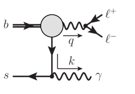
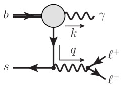
Figure 2: The LP $A$-type and $B$-type insertions. The grey blob denotes the effective hard vertex of the operators $P_{1,\ldots,8}$.

3.1.1 Effective hard vertex

We begin the discussion of the first matching step to SCET${}_{\text{I}}$ by assuming that $q^{2}$ is hard and the insertion is of the $A$-type. A LP contribution to the hadronic tensors $T_{i}^{\mu\nu}$ is obtained only when the separation $x$ between the electromagnetic current $j^{\mu}_{f}(x)$ and the operator $P_{i}(0)$ is of order $1/\sqrt{E_{\gamma}\Lambda_{\rm QCD}}$. In other words, the propagator joining the two vertices in the left diagram of Figure 2 must have hard-collinear virtuality, since a hard propagator would lead to power-suppression. Integrating out the hard scale therefore results in an effective flavour-changing vertex, represented by the grey circle in Figure 2. The hadronic tensors appearing in (2.5) are therefore matched to SCET${}_{\text{I}}$ as follows:

$$\sum_{i=1}^{9}\eta_{i}C_{i}T_{i}^{\mu\nu} =\sum_{i=1}^{9}C_{i}\,H_{i}(q^{2})\int\!d^{4}x\,e^{ikx}\,\big{\langle}{0}\big{|}\text{T}\{j^{\mu}_{f,\,\rm SCET_{\rm I}}(x),\,[{\overline{q}}_{\rm hc}\gamma^{\nu_{\perp}}P_{L}h_{v}](0)\}\big{|}{{\overline{B}}_{q}}\big{\rangle}\,,$$ (3.3)

$$C_{10}T_{10}^{\mu\nu} =C_{10}\,H_{10}(q^{2})\int\!d^{4}x\,e^{ikx}\,\big{\langle}{0}\big{|}\text{T}\{j^{\mu}_{f,\,\rm SCET_{\rm I}}(x),\,[{\overline{q}}_{\rm hc}\gamma^{\nu_{\perp}}P_{L}h_{v}](0)\}\big{|}{{\overline{B}}_{q}}\big{\rangle}\,,$$ (3.4)

where $H_{i}(q^{2})$ denotes the hard matching coefficients, and the hadronic tensor for $i=7$ is $T_{7A}^{\mu\nu}$. All operators match to the same correlation function of the SCET${}_{\text{I}}$ heavy-to-light current ${\overline{q}}_{\rm hc}\gamma^{\nu_{\perp}}P_{L}h_{v}$ and the representation of the SCET${}_{\text{I}}$ electromagnetic current. In the above equation the Wilson coefficients $C_{i}$ are evaluated at the scale $\nu\sim m_{b}$ after evolving them to $\nu$ from the electroweak scale. The matching coefficients $H_{i}$ are determined at the hard scale $\mu_{h}\sim m_{b}$ in the matching QCD$\,\to\,$SCET${}_{\text{I}}$. In addition to $q^{2}$, they depend on the scale $\nu$ through the ultraviolet divergences of the QCD diagrams, such that the dependence on $\nu$ cancels in the product $C_{i}(\nu)H_{i}(\nu,\mu_{h})$, as well as on the scale $\mu_{h}$ through the infrared divergences of the QCD diagrams. The $\mu_{h}$-dependence cancels with the dependence on $\mu_{h}$ of the SCET${}_{\text{I}}$ correlation functions in (3.3), (3.4).

The $\mathcal{O}(\alpha_{s})$ corrections to the hard functions $H_{i}(q^{2})$ are identical to those for $B\to K^{(*)}\ell\bar{\ell}$ (see Figure 2 in [25]). For the four-quark operators, they arise from two-loop diagrams. It is customary to absorb the four-quark operator contributions into effective Wilson coefficients of $P_{7-9}$, and we follow this practice here. Hence we define

$$\sum_{i=1}^{9}C_{i}\,H_{i}(q^{2}) \equiv V_{9}^{\rm eff}(q^{2})+\frac{2\,{\overline{m}}_{b}\,m_{B_{q}}}{q^{2}}\,V^{\rm eff}_{7}(q^{2}),$$ (3.5)

$$C_{10}\,H_{10}(q^{2}) \equiv V^{\rm eff}_{10}(q^{2}),$$

where ${\overline{m}}_{b}$ denotes the ${\overline{\text{MS}}}$-scheme $b$-quark mass at the scale $\nu$. The effective hard functions including the $\mathcal{O}(\alpha_{s})$ correction are then given by

$$V_{7}^{\text{eff}}=\; C_{7}^{\text{eff}}\,C_{T_{1}}^{(A0)}-\frac{\alpha_{s}}{4\pi}\bigg{[}C_{1}\bigg{(}F_{1}^{(7c)}+\frac{\lambda_{u}^{(q)}}{\lambda_{t}^{(q)}}\left[F_{1}^{(7c)}-F_{1}^{(7u)}\right]\bigg{)}$$

$$+\,C_{2}\bigg{(}F_{2}^{(7c)}+\frac{\lambda_{u}^{(q)}}{\lambda_{t}^{(q)}}\left[F_{2}^{(7c)}-F_{2}^{(7u)}\right]\bigg{)}+C_{8}^{\text{eff}}F_{8}^{(7)}+\text{$C_{3-6}$-terms}\,\bigg{]}\,,$$ (3.6)

$$V_{9}^{\text{eff}}=\; C_{9}^{\text{eff}}(q^{2})\,C_{V}^{(A0)}-\frac{\alpha_{s}}{4\pi}\bigg{[}C_{1}\bigg{(}F_{1}^{(9c)}+\frac{\lambda_{u}^{(q)}}{\lambda_{t}^{(q)}}\left[F_{1}^{(9c)}-F_{1}^{(9u)}\right]\bigg{)}$$

$$+\,C_{2}\bigg{(}F_{2}^{(9c)}+\frac{\lambda_{u}^{(q)}}{\lambda_{t}^{(q)}}\left[F_{2}^{(9c)}-F_{2}^{(9u)}\right]\bigg{)}+C_{8}^{\text{eff}}F_{8}^{(9)}+\text{$C_{3-6}$-terms}\,\bigg{]}\,,$$ (3.7)

$$V_{10}^{\text{eff}}=\; C_{10}\,C_{V}^{(A0)},$$ (3.8)

where we have suppressed all arguments $q^{2},\mu_{h},\nu$. Here $\alpha_{s}$ is evaluated at $\mu_{h}$. The effective Wilson coefficient combinations read as follows [30, 31]:

$$C_{7}^{\text{eff}} =C_{7}-\frac{C_{3}}{3}-\frac{4}{9}C_{4}-\frac{20}{3}C_{5}-\frac{80}{9}C_{6},$$ (3.9)

$$C_{8}^{\text{eff}} =C_{8}+\,C_{3}\,-\frac{1}{6}C_{4}+20C_{5}-\frac{10}{3}C_{6},$$ (3.10)

$$C_{9}^{\text{eff}}(q^{2}) =C_{9}+Y(q^{2})-\frac{\lambda_{u}^{(q)}}{\lambda_{t}^{(q)}}\left(\frac{4}{3}C_{1}+C_{2}\right)\big{[}h(q^{2},0)-h(q^{2},m_{c})\big{]}.$$ (3.11)

We use the definition of the function $Y(q^{2})$ from [25]. The function $h(q^{2},m_{q})$ [31] depends on the light quark masses $m_{u,d}$, which are set to zero, or the charm-quark pole mass $m_{c}$.

For the semileptonic operators and the parts from the four-quark operators contained in the effective Wilson coefficients above, the NLO QCD corrections are contained in the matching coefficients $C_{V}^{(A0)}(q^{2})$, $C_{T_{1}}^{(A0)}(q^{2})$ of the heavy-to-light (axial-) vector and tensor QCD currents to the SCET${}_{\text{I}}$ current ${\overline{q}}_{\text{hc}}\gamma^{\nu_{\perp}}P_{L}h_{v}$ [36]. We use the notation of [37] and provide the NLO expression here:

$$C_{V}^{(A0)}(q^{2}) =1+\frac{\alpha_{s}(\mu)C_{F}}{4\pi}\,\bigg{(}$$

$$-2\ln^{2}\frac{m_{B_{q}}z}{\mu}+5\ln\frac{m_{B_{q}}z}{\mu}-\frac{3-2z}{1-z}\ln z-2\operatorname{Li_{2}}2(1-z)-\frac{\pi^{2}}{12}-6\bigg{)}\,,$$ (3.12)

$$C_{T_{1}}^{(A0)}(q^{2}) =1+\frac{\alpha_{s}(\mu)C_{F}}{4\pi}\,\bigg{(}$$

$$2\ln\frac{m_{b}}{\nu}-2\ln^{2}\frac{m_{B_{q}}z}{\mu}+5\ln\frac{m_{B_{q}}z}{\mu}-3\ln z-2\operatorname{Li_{2}}2(1-z)-\frac{\pi^{2}}{12}-6\bigg{)}\,,$$ (3.13)

with $z=1-q^{2}/m_{B_{q}}^{2}$, $C_{F}=(N_{c}^{2}-1)/(2N_{c})=4/3$, and $N_{c}=3$ in QCD.

The NLO QCD corrections from the charged-current operators $P_{1,2}^{u,c}$ and $P_{8}$ are given by $F^{(7u,7c,9u,9c)}_{1,2}(q^{2})$ from [38, 39, 40] and $F_{8}^{7,9}(q^{2})$ from [39, 25], respectively. The analogous corrections from $P_{3,4,5,6}$ labelled “$C_{3-6}$-terms” in (3.1.1), (3.1.1) are suppressed by the small penguin-operator Wilson coefficients and have been neglected here. The terms proportional to $\lambda_{u}^{(q)}$ in $V_{7,9}^{\text{eff}}$ give rise to direct CP violation, which is doubly-Cabibbo suppressed for $q=s$ and leads to tiny CP asymmetries, whereas for $q=d$ CP-violating effects can be larger.

To summarize the discussion up to this point, we note that the $A$-type contribution to $B_{q}\to\gamma\ell\bar{\ell}$ amplitude (2.5) after matching to SCET${}_{\text{I}}$ at LP is obtained in the form

$${\overline{\mathcal{A}}}_{\text{type}-A}=\; ie\,\frac{\alpha_{\text{em}}}{4\pi}\,\mathcal{N}_{\text{ew}}\,\epsilon^{\star}_{\mu}\left\{\left(V_{9}^{\text{eff}}(q^{2})+\frac{2\,{\overline{m}}_{b}\,m_{B_{q}}}{q^{2}}\,V^{\text{eff}}_{7}(q^{2})\right)L_{V,\nu}+V^{\text{eff}}_{10}(q^{2})L_{A,\nu}\right\}$$

$$\times\int\!d^{4}x\,e^{ikx}\,\big{\langle}{0}\big{|}\text{T}\{j^{\mu}_{f,\,\rm SCET_{\rm I}}(x),\,[{\overline{q}}_{\text{hc}}\gamma^{\nu_{\perp}}P_{L}h_{v}](0)\}\big{|}{{\overline{B}}_{q}}\big{\rangle}\,.$$ (3.14)

The derivation of this result assumed that the lepton-pair virtuality is hard. When $q^{2}$ is anti-hard-collinear, the structure of the result remains the same. However, the effective vertices, which are functions of $q^{2}/m_{b}^{2}$, could now be evaluated at $q^{2}=0$, since the ratio $q^{2}/m_{b}^{2}$ is power-suppressed. More importantly, the effective vertex $V_{7}^{\text{eff}}(q^{2})$ becomes power-enhanced due to the photon pole $1/q^{2}$, relative to which $V_{9,10}^{\text{eff}}(q^{2})$ should be dropped as power-suppressed. This, however, results in a physically unacceptable approximation. For example, making the same approximation for the exclusive $B\to K^{(*)}\ell\bar{\ell}$ decay, the lepton forward-backward asymmetry would disappear and the predicted branching fractions and angular distributions in the small-$q^{2}$ region become unrealistic. The reason is that the magnitude of the Wilson coefficients $C_{9,10}$ is about an order of magnitude larger than $C_{7}$, so that it is more appropriate to count $C_{9,10}\sim m_{b}^{2}/q^{2}\times C_{7}$. In other words, the expansion in $1/m_{b}$ should be performed for the $C_{9,10}$ and $C_{7}$ terms separately, and for each term the LP should be kept. In the same spirit, no harm is done by keeping the $q^{2}$-dependence in the effective vertices also at small $q^{2}$. In this way, one obtains a smooth interpolation between hard and anti-hard-collinear $q^{2}$, as (3.14) applies without modification to the anti-hard-collinear, small-$q^{2}$ region. This is also the procedure that has been adopted for the exclusive $B\to K^{(*)}\ell\bar{\ell}$ [25], which forms the basis of the QCD phenomenology of this decay.

Another subtlety needs to be mentioned here. When $q^{2}$ is anti-hard-collinear, the effective hard vertices are no longer guaranteed to be dominated by hard virtualities. This is obvious for the one-loop four-quark operator contribution shown in the left diagram of Figure 1, where the quark-loop is then purely anti-hard-collinear. At $\mathcal{O}(\alpha_{s})$ the two-loop diagrams contributing to $F_{1,2}^{(7u,7c,9u,9c)}$ contain hard and hard-collinear regions. It therefore appears that the previous treatment should be substantially modified, since only the hard regions are integrated out in the first matching step to SCET${}_{\text{I}}$. However, the SCET${}_{\text{I}}$ correlation function in (3.14) is governed by (hard-)collinear physics. The anti-(hard-)collinear and the (hard-)collinear sectors of SCET${}_{\text{I}}$ are already decoupled after integrating out the hard modes and performing the soft-decoupling transformation in SCET${}_{\text{I}}$. The soft Wilson lines from the decoupling transformation cancel, as the anti-collinear final state is colour-neutral, hence the existence of the anti-hard-collinear physics leaves no impact on the remaining collinear and soft interactions. In consequence, when $q^{2}$ is anti-hard-collinear, we may simply assume that the hard functions $H_{i}(q^{2})$ introduced above are in fact the hard and anti-hard-collinear functions. In principle, these functions may therefore contain formally large logarithms $\ln q^{2}/m_{b}^{2}$, which we cannot resum by not factorizing the hard and anti-hard-collinear physics properly. However, the existence of the limit $q^{2}\to 0$ shows that such logarithms are absent, at least at LP and $\mathcal{O}(\alpha_{s})$. We note that the same discussion applies to the standard treatment of the exclusive $B\to K^{(*)}\ell\bar{\ell}$ mode, although we are not aware of its explicit mentioning.

In addition to the $A$-type insertion, there is also a $B$-type contribution, see the right diagram of Figure 2, in which the role of the real and virtual photon is interchanged. When $q^{2}$ is anti-hard-collinear, the separation between the flavour-changing and electromagnetic current is again of order $1/(E_{\gamma}\Lambda_{\text{QCD}})$, and one obtains a LP contribution. Since the lepton-pair originates from the electromagnetic current, there is no $B$-type contraction from the operator $P_{9,10}$, and in fact no contribution from the corresponding effective vertices $V^{\text{eff}}_{9,10}$. Hence

$${\overline{\mathcal{A}}}_{\text{type}-B}=\, ie\,\frac{\alpha_{\text{em}}}{4\pi}\,\mathcal{N}_{\text{ew}}\,\epsilon^{\star}_{\mu}\frac{4\,{\overline{m}}_{b}E_{\gamma}}{q^{2}}\,V^{\text{eff}}_{7}(0)L_{V,\nu}$$

$$\times\int\!d^{4}x\,e^{iqx}\,\big{\langle}{0}\big{|}\text{T}\{j^{\nu}_{f,\,\rm SCET_{\rm I}}(x),\,[{\overline{q}}_{{\overline{\rm hc}}}\gamma^{\mu_{\perp}}P_{L}h_{v}](0)\}\big{|}{{\overline{B}}_{q}}\big{\rangle}\,.$$ (3.15)

We note that the effective vertex $V^{\text{eff}}_{7}(0)$ is now evaluated for $k^{2}=0$, and the Fourier transform of the SCET${}_{\text{I}}$ correlation function is taken with respect to $q$ rather than $k$. The remarks above concerning the interpretation of the “hard” functions $H_{i}(q^{2})$ when the argument $q^{2}$ is anti-hard-collinear, apply to the present case $k^{2}=0$.

When $q^{2}$ is hard, the SCET${}_{\text{I}}$ correlation function in (3.15) is not the correct expression, since the distance $x\sim 1/\sqrt{q^{2}}$ is hard and should already have been integrated out in the matching to SCET${}_{\text{I}}$. In other words, the propagator connecting the two currents in the right diagram of Figure 2 is far off-shell and should be contracted to a point, resulting in a local operator rather than a SCET${}_{\text{I}}$ correlation function. Also the vertex $V^{\text{eff}}_{7}(0)$ is not necessarily the correct one in (3.15), since it was obtained by matching the flavour-changing current with an on-shell out-going quark. On the other hand, the off-shell propagator provides power suppression of the $B$-type contraction in the hard-$q^{2}$ region relative to the anti-hard-collinear one, such that $B$-type insertions are NLP effects for hard $q^{2}$, for which we aim only at $\mathcal{O}(\alpha_{s}^{0})$ accuracy.

We now argue that within the approximation that we include only LO $\mathcal{O}(\alpha_{s}^{0})$ contributions at NLP, the expression (3.15) can be used even when $q^{2}$ is hard. The $B$-type insertion $\mathcal{O}(\alpha_{s}^{0})$ diagram (the diagram corresponding to the middle diagram of Figure 1 but with the quark-loop replaced by the direct attachment of the photon to the flavour-changing vertex) contains the expression

$${\overline{v}}_{s}(l)\,\gamma^{\nu}\frac{i(\not{q}-\not{l})}{q^{2}-2q\cdot l}\left[\gamma^{\mu},\not{k}\right]P_{R}u_{b}(p_{b})\,\epsilon^{*}_{\mu}(k)\,,$$ (3.16)

where $l$ is the momentum of the spectator quark. The LP approximation in both $q^{2}$ regions is obtained from keeping only the potentially large momentum components in the numerator. For hard $q^{2}$ this includes $(n_{+}q)\frac{\not{n}_{-}}{2}$. The important observation is that this term vanishes, since $\mu$ is transverse and $k=E_{\gamma}n_{-}$, hence $\not{n}_{-}\left[\gamma^{\mu_{\perp}},\not{n}_{-}\right]=0$. Thus, the previous equation simplifies to

$$\frac{1}{2}\,{\overline{v}}_{s}(l)\,\gamma^{\nu}\frac{i(n_{-}q)\not{n}_{+}}{q^{2}-2q\cdot l}\left[\gamma^{\mu},\not{k}\right]P_{R}u_{b}(p_{b})\,\epsilon^{*}_{\mu}(k)$$ (3.17)

in both $q^{2}$-regions. Eq. (3.17) would be obtained from (3.15) in the anti-hard-collinear $q^{2}$ region, which proves that we can smoothly extrapolate (3.15) into the hard region at $\mathcal{O}(\alpha_{s}^{0})$, in which case

$$\frac{n_{-}q}{q^{2}-2q\cdot l} \to\frac{1}{n_{+}q}\,.$$ (3.18)

Since we do not aim at $\mathcal{O}(\alpha_{s})$ accuracy at NLP, we can use (3.15) in the hard-collinear and hard $q^{2}$ region, even if in the hard region the $\mathcal{O}(\alpha_{s})$ correction to $V_{7}^{\text{eff}}(0)$ is not the complete one at NLO in $\alpha_{s}$.

To summarize the first matching step, we obtain the LP $B_{q}\to\gamma\ell\bar{\ell}$ amplitude (2.5) in the form

$${\overline{\mathcal{A}}}_{\text{LP}} ={\overline{\mathcal{A}}}_{\text{type}-A}+{\overline{\mathcal{A}}}_{\text{type}-B}\,,$$ (3.19)

where the two terms are given by (3.14), (3.15). The second step consists of matching the SCET${}_{\text{I}}$ correlation function in these terms to SCET${}_{\text{II}}$ by integrating out the hard-collinear modes. Before turning to this task in the following subsection, we mention that the same correlation function appears for all operators $P_{i}$ from the electroweak effective Lagrangian. The RG evolution from the hard to the hard-collinear scale is therefore universally related to the anomalous dimension of the LP A0-type SCET${}_{\text{I}}$ heavy-to-light current ${\overline{q}}_{\text{hc}}\gamma^{\nu_{\perp}}P_{L}h_{v}$ [36] and equals the one that appears in the $B_{u}\to\gamma\ell\bar{\nu}_{\ell}$ decay. We therefore have

$$V_{i}^{\text{eff}}(q^{2},\mu_{hc},\nu) =U_{H}(q^{2},\mu_{hc},\mu_{h})\,V_{i}^{\text{eff}}(q^{2},\mu_{h},\nu)\,.$$ (3.20)

The RG equation for $U_{H}(q^{2},\mu_{hc},\mu_{h})$ and its solution to NLL can be found in Eqs. (A.1) and (A.3) of [20] with $U_{H}(q^{2},\mu_{hc},\mu_{h})=U_{1}((m_{B_{q}}^{2}-q^{2})/(2m_{B_{q}}),\mu_{h},\mu_{hc})$ in terms of the evolution factor defined there.

3.1.2 Hard-collinear function

The matching of SCET${}_{\text{I}}$ to SCET${}_{\text{II}}$ amounts to integrating out the hard-collinear modes in the SCET${}_{\text{I}}$ correlation function

$$\mathcal{T}^{\mu\nu}(r)\equiv\int\!d^{4}x\,e^{irx}\,\big{\langle}{0}\big{|}\text{T}\{j^{\mu}_{f,\,\text{SCET${}_{\text{I}}${}}}(x),\,[{\overline{q}}_{\text{hc}}\gamma^{\nu_{\perp}}P_{L}h_{v}](0)\}\big{|}{{\overline{B}}_{q}}\big{\rangle}\,.$$ (3.21)

No new calculation is required in this step. For $r^{2}=0$, it has first been explained and computed to the one-loop order for $B_{u}\to\gamma\ell\bar{\nu}_{\ell}$ in [18, 19]. The generalization to $r^{2}\neq 0$ needed here was worked out in [22].

We recall from [18] that the SCET${}_{\text{I}}$ electromagnetic current $j^{\mu}_{q,\text{SCET${}_{\text{I}}${}}}(x)$ relevant here consists of two power-suppressed pieces

$$j^{\mu}_{q,\text{SCET${}_{\text{I}}${}}}(x)=\; j^{(0)\mu}_{q,\text{SCET${}_{\text{I}}${}}}(x)+j^{(1)\mu}_{q,\text{SCET${}_{\text{I}}${}}}(x)$$

$$=\; \sum_{q}Q_{q}\left[{\overline{q}}_{\text{hc}}\left(\gamma_{\perp}^{\mu}\frac{1}{i{n_{+}}D_{\text{hc}}}i\not{D}_{\text{hc}\perp}+i\not{D}_{\text{hc}\perp}\frac{1}{i{n_{+}}D_{\text{hc}}}\gamma_{\perp}^{\mu}\right)\frac{{\not{n}}_{+}}{2}q_{\text{hc}}\right](x)$$

$$+\sum_{q}Q_{q}\left[{\overline{q}}_{s}(x_{-})\,\gamma^{\mu}_{\perp}\,q_{\text{hc}}(x)\right]$$ (3.22)

with $x_{-}^{\mu}\equiv({n_{+}}x)\,n_{-}^{\mu}/2$. Here (and above) $q_{\text{hc}}=W^{\dagger}\xi_{\text{hc}}$ is the hard-collinear quark field multiplied by the QCD hard-collinear Wilson line. The second term on the right-hand side describes the conversion of the soft spectator quark into a hard-collinear quark at the photon vertex and counts as $\mathcal{O}(\lambda^{2})$. The first term is only $\mathcal{O}(\lambda)$ suppressed, but contributes to the amplitude with an external soft quark only through the $\mathcal{O}(\lambda)$ suppressed quark-gluon vertex of the SCET Lagrangian, that converts a soft quark into a hard-collinear quark through interaction with a hard-collinear gluon. This part of the current contributes to the matching only from NLO in the $\alpha_{s}$ expansion through hard-collinear gluon corrections to the photon vertex.

With the hard-collinear physics at the scale $E_{\gamma}\Lambda_{\text{QCD}}$, $m_{b}\Lambda_{\text{QCD}}$ integrated out, the remaining nonperturbative soft physics is parametrized at LP in the matching by the leading-twist light-cone distribution amplitude of the $B$ meson, $\phi_{+}(\omega)$. The matching equation reads

$$\mathcal{T}^{\mu\nu}(r)=(g_{\perp}^{\mu\nu}+i\varepsilon_{\perp}^{\mu\nu})\,\frac{Q_{q}F_{B_{q}}m_{B_{q}}}{4}\,\int_{0}^{\infty}\!\!d\omega\,\phi_{+}(\omega)\,\frac{J(n\cdot r,r^{2},\omega)}{\omega-r^{2}/n\cdot r-i0^{+}}\,.$$ (3.23)

Since both cases will be needed, we employ the convention that $n\cdot r$ denotes the large component $n_{+}r$, when $r$ is a collinear momentum and $n_{-}r$ when it is anti-collinear. Concretely, for the $A$-type contribution, we need $J(n_{+}k,0,\omega)$ with $n_{+}k=2E_{\gamma}$, while for the $B$-type one the relevant function is $J(n_{-}q,q^{2},\omega)$ with $n_{-}q=m_{B_{q}}$ and $q^{2}=m_{B_{q}}(m_{B_{q}}-2E_{\gamma})$.

The scale-dependent quantities $F_{B_{q}}$, $J$, $\phi_{+}$ are assumed to be evaluated at the hard-collinear scale $\mu_{hc}$, and the scale argument has been omitted in (3.23). Their definitions are as follows. The $B$-meson LCDA $\phi_{+}(\omega)$ [42, 43] is the Fourier transform of the HQET matrix element

$$\big{\langle}{0}\big{|}{\overline{q}}_{s}(t{n_{-}})\,[t{n_{-}},0]\,{\not{n}}_{-}\!\gamma_{5}\,h_{v}(0)\,\big{|}{{\overline{B}}_{q}(p)}\big{\rangle} =im_{B_{q}}F_{B_{q}}\int_{0}^{\infty}\!\!\!d\omega\,e^{-i\omega t}\,\phi_{+}(\omega)\,,$$ (3.24)

where $[t{n_{-}},0]$ denotes a straight soft Wilson line connecting the light-like separated points 0 and $t{n_{-}}$. It is customary to relate the HQET $B$-meson decay constant $F_{B_{q}}$ to the scale-independent decay constant of full QCD $f_{B_{q}}$, introduced in (2.6), and use the latter as an input. The relation is

$$F_{B_{q}}(\mu_{hc}) =U_{F}^{-1}(\mu_{hc},\mu_{h})\,K^{-1}(\mu_{h})\,f_{B_{q}}\,$$ (3.25)

with

$$K^{-1}(\mu) =1+\frac{\alpha_{s}(\mu)C_{F}}{4\pi}\left(\frac{3}{2}\ln\frac{\mu^{2}}{m_{b}^{2}}+2\right).$$ (3.26)

The RG evolution factor $U_{F}^{-1}$ from $\mu_{hc}$ to $\mu_{h}$ can be obtained from the Appendix of [20] with the identification $U_{F}^{-1}(\mu_{hc},\mu_{h})=U_{2}^{-1}(\mu_{h},\mu_{hc})$ in terms of the evolution factor defined there.

Finally, the hard-collinear matching function (“jet function”) reads [22]

$$J(n\cdot r,r^{2},\omega;\mu)=\; 1+\frac{\alpha_{s}C_{F}}{4\pi}\,\Bigg{\{}\ln^{2}\frac{\mu^{2}}{n\cdot r\,(\omega-{\overline{n}}\cdot r)}-\frac{\pi^{2}}{6}-1$$

$$-\,\frac{{\overline{n}}\cdot r}{\omega}\ln\frac{{\overline{n}}\cdot r-\omega}{{\overline{n}}\cdot r}\left[\ln\frac{\mu^{2}}{-r^{2}}+\ln\frac{\mu^{2}}{n\cdot r\,(\omega-{\overline{n}}\cdot r)}+3\right]\Bigg{\}}$$ (3.27)

with ${\overline{n}}\cdot r=r^{2}/n\cdot r$. We note that the second line vanishes for $r^{2}=0$. Hence for the $A$-type insertions, the convolution $J(\omega)\otimes\phi_{+}(\omega)$ in (3.23) can be expressed as

$$\int_{0}^{\infty}\frac{d\omega}{\omega}\,J(2E_{\gamma},0,\omega;\mu)\,\phi_{+}(\omega;\mu)$$

$$=\,\frac{1}{\lambda_{B_{q}}(\mu)}\Bigg{[}1+\frac{\alpha_{s}(\mu)C_{F}}{4\pi}\left(\ln^{2}\frac{2E_{\gamma}\mu_{0}}{\mu^{2}}-2\sigma^{(1)}_{B_{q}}(\mu)\ln\frac{2E_{\gamma}\mu_{0}}{\mu^{2}}+\sigma^{(2)}_{B_{q}}(\mu)-\frac{\pi^{2}}{6}-1\right)\Bigg{]}\qquad$$ (3.28)

in terms of the inverse ($\lambda_{B_{q}}$) and the first two inverse-logarithmic moments ($\sigma^{(1,2)}_{B_{q}}$)

$$\sigma^{(n)}_{B_{q}}(\mu) =\int_{0}^{\infty}\!\!d\omega\,\frac{\lambda_{B_{q}}(\mu)}{\omega}\ln^{n}\frac{\mu_{0}}{\omega}\,\phi_{+}(\omega,\mu), \sigma^{(0)}_{B_{q}} \equiv 1$$ (3.29)

of the $B$-meson LCDA [20]. However, for the $B$-type insertions the expression is more complicated and the entire function $\phi_{+}(\omega)$ must be known to evaluate the convolution integral.

3.1.3 Final factorized form

Putting together (3.14), (3.15) and (3.23), we obtain the following compact result for the LP $B_{q}\to\gamma\ell\bar{\ell}$ amplitude (2.5):

$${\overline{\mathcal{A}}}_{{\rm LP}} = ie\,\frac{\alpha_{\text{em}}}{4\pi}\,\mathcal{N}_{\text{ew}}\,\epsilon^{\star}_{\mu}\,(g_{\perp}^{\mu\nu}+i\varepsilon_{\perp}^{\mu\nu})\,\frac{Q_{q}F_{B_{q}}E_{\gamma}}{2}\,\Bigg{\{}$$ (3.30)

$$\left\{\left(V_{9}^{\rm eff}(q^{2})+\frac{2\,{\overline{m}}_{b}\,m_{B_{q}}}{q^{2}}\,V^{\rm eff}_{7}(q^{2})\right)L_{V,\nu}+V^{\rm eff}_{10}(q^{2})L_{A,\nu}\right\}\frac{m_{B_{q}}}{2E_{\gamma}}\,\int_{0}^{\infty}\!\frac{d\omega}{\omega}\,\phi_{+}(\omega)\,J(2E_{\gamma},0,\omega)$$

$$+\,\frac{2\,{\overline{m}}_{b}\,m_{B_{q}}}{q^{2}}\,V^{\rm eff}_{7}(0)L_{V,\nu}\,\int_{0}^{\infty}\!\!d\omega\,\phi_{+}(\omega)\frac{J(m_{B_{q}},q^{2},\omega)}{\omega-q^{2}/m_{B_{q}}-i0^{+}}\Bigg{\}}\,.$$

Note that the amplitude contains $g_{\perp}^{\mu\nu}+i\varepsilon_{\perp}^{\mu\nu}$ and not $g_{\perp}^{\mu\nu}-i\varepsilon_{\perp}^{\mu\nu}$. From (2.15) this implies

$$F_{R}^{(i,\text{LP})}=0,\qquad i=1,\ldots,10,$$ (3.31)

and the so-called form-factor-symmetry relation $F_{V}^{(i)}=F_{A}^{(i)}$ as a consequence of helicity conservation in the heavy-quark and large-energy limit.

For completeness, we also give the left-handed form factors. For this purpose we define

$$\sum_{i=7,9}F_{L}^{(i\text{-eff},\text{LP})} \equiv\sum_{i=1}^{9}\eta_{i}C_{i}F_{L}^{(i,\text{LP})}, F_{L}^{(10\text{-eff},\text{LP})} \equiv\eta_{10}C_{10}F_{L}^{(10,\text{LP})}$$ (3.32)

and find

$$F_{L}^{(7\text{-eff},\text{LP})}=\; \frac{Q_{q}F_{B_{q}}}{2}\,\frac{2\,{\overline{m}}_{b}\,m_{B_{q}}}{q^{2}}\,\Bigg{\{}V^{\text{eff}}_{7}(q^{2})\frac{m_{B_{q}}}{2E_{\gamma}}\,\int_{0}^{\infty}\!d\omega\,\phi_{+}(\omega)\,\frac{J(2E_{\gamma},0,\omega)}{\omega}$$

$$+V^{\text{eff}}_{7}(0)\,\int_{0}^{\infty}\!d\omega\,\phi_{+}(\omega)\frac{J(m_{B_{q}},q^{2},\omega)}{\omega-q^{2}/m_{B_{q}}-i0^{+}}\Bigg{\}}\,,$$ (3.33)

$$F_{L}^{(i\text{-eff},\text{LP})}=\; \frac{Q_{q}F_{B_{q}}}{2}\,V^{\rm eff}_{i}(q^{2})\,\frac{m_{B_{q}}}{2E_{\gamma}}\,\int_{0}^{\infty}\!d\omega\,\phi_{+}(\omega)\,\frac{J(2E_{\gamma},0,\omega)}{\omega}\qquad i=9,10\,.$$ (3.34)

We recover the result for $B_{u}\to\gamma\ell\bar{\nu}_{\ell}$ [20] from (3.34), by setting $C_{9}=1$ and $C_{i}=0$ otherwise.

3.2 Form factors at NLP

As for the case of $B_{u}\to\gamma\ell\bar{\nu}_{\ell}$ [20] we include NLP $\Lambda_{\text{QCD}}/E_{\gamma}$, $\Lambda_{\text{QCD}}/m_{b}$ corrections to the above $B_{q}\to\gamma\ell\bar{\ell}$ form factors, but we aim only at $\mathcal{O}(\alpha_{s}^{0})$ accuracy at NLP. Such power corrections arise from three sources:

• The coupling of the real or virtual photon to the heavy quark.

• Power corrections to the (anti-) hard-collinear light-quark propagator in the LP $\mathcal{O}(\alpha_{s}^{0})$ contributions, that is, power corrections to the SCET${}_{\text{I}}$ correlation function (3.21) at tree level.

• Annihilation-type insertions of the four-quark operators, such that the real and the virtual photon are attached to the quark loop, see the right diagram in Figure 1.

The first two effects are also present in $B_{u}\to\gamma\ell\bar{\nu}_{\ell}$. The chromomagnetic dipole operator $P_{8}$ can be ignored, since its insertions involve at least one power of $\alpha_{s}$.

The NLP contributions from the semileptonic operators $P_{i}$ ($i=9,10$) can be taken directly from the $B_{u}\to\gamma\ell\bar{\nu}_{\ell}$ calculation [20]:

$$F_{L}^{(i,\text{NLP})} =\frac{\xi_{B_{q}}(E_{\gamma})}{2},$$ (3.35)

$$F_{R}^{(i,\text{NLP})} =\frac{f_{B_{q}}}{4E_{\gamma}}\left(Q_{b}\frac{m_{B_{q}}}{m_{b}}+Q_{q}\frac{m_{B_{q}}}{2E_{\gamma}}\right).$$ (3.36)

At NLP the right-helicity form factor is non-vanishing, but this “symmetry-breaking” contribution (as it implies $F_{V}\neq F_{A}$) is local at $\mathcal{O}(\alpha_{s}^{0})$. By this we mean that at this order they can be expressed in terms of the $B$-meson decay constant. On the other hand, the power correction to the left-helicity form factor cannot be factorized and is parametrized by an unknown function, the “symmetry-preserving” soft form factor. We also refer to these contributions as “non-local” power corrections. For $q=u$ relevant to $B_{u}\to\gamma\ell\bar{\nu}_{\ell}$ it has been calculated with QCD sum rules [21, 22, 24]. The definition in (3.35) is such that in the SU(3)-flavour symmetry limit of QCD $\xi_{B_{q}}=Q_{q}/Q_{u}\times\xi_{B_{u}}$ ($q=d,s$) is related to the one introduced in [20] for $B_{u}\to\gamma\ell\bar{\nu}_{\ell}$ simply by the ratio of the electric charges of the spectator quarks. We remark that we consistently set the strange-quark mass to zero in our analysis, which would otherwise give $m_{s}/(2E_{\gamma})$ corrections to the above expressions.

The NLP contributions of $P_{7}$ from the $A$-type insertion are

$$F_{L}^{(7A,\text{NLP})} =-\frac{{\overline{m}}_{b}\,m_{B_{q}}}{q^{2}}\left(\xi_{B_{q}}(E_{\gamma})+Q_{b}\frac{f_{B_{q}}}{2E_{\gamma}}\right),$$ (3.37)

$$F_{R}^{(7A,\text{NLP})} =-Q_{q}\frac{{\overline{m}}_{b}f_{B_{q}}}{(2E_{\gamma})^{2}}\,.$$ (3.38)

We note that the emission of the photon from the heavy quark is symmetry-preserving for $P_{7}$. For the $B$-type insertion of $P_{7}$ we find

$$F_{L}^{(7B,\text{NLP})} =-\frac{{\overline{m}}_{b}\,m_{B_{q}}}{q^{2}}\left(\widetilde{\xi}_{B_{q}}(E_{\gamma})+Q_{b}\frac{f_{B_{q}}}{2E_{\gamma}}\right),$$ (3.39)

$$F_{R}^{(7B,\text{NLP})} =0\,.$$ (3.40)

The parameterization of the NLP $B$-type insertion requires another soft form factor $\widetilde{\xi}_{B_{q}}(E_{\gamma})$. The SCET${}_{\text{I}}$ correlation function (3.21) can be considered as a function of $n\cdot r$ and $r^{2}$, where $n\cdot r$ is the large component of the (anti-)collinear momentum $r$. To parametrize the NLP correction, we may introduce the soft form factor $\zeta_{B_{q}}(n\cdot r,r^{2})$ of two variables. Similar to the general hard-collinear function $J(n\cdot r,r^{2},\omega)$ in (3.23), the soft-form factors in (3.37), (3.39) are then the special cases

$$\xi_{B_{q}}(E_{\gamma}) =\zeta_{B_{q}}(2E_{\gamma},0), \widetilde{\xi}_{B_{q}}(E_{\gamma}) =\zeta_{B_{q}}(m_{B_{q}},m_{B_{q}}(m_{B_{q}}-2E_{\gamma}))\,.$$ (3.41)

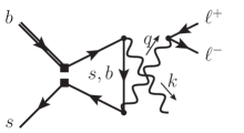
Figure 3: Annihilation-type one-loop diagrams with insertions of the four-quark operators $P_{1,2}^{(u,c)},P_{3-6}$. The operator insertion is depicted by black squares. The $Q$ stands for the five quark flavours $u,d,s,c,b$.

The effect of the four-quark operators at $\mathcal{O}(\alpha_{s}^{0})$ is two-fold. First, the NLP terms from the left and middle diagram of Figure 1 replace $C_{7}$ and $C_{9}$ multiplying $F_{L,R}^{(7A,\text{NLP})}$, $F_{L,R}^{(7B,\text{NLP})}$, $F_{L,R}^{(9,\text{NLP})}$ above by $C_{7}^{\text{eff}}$ and $C_{9}^{\text{eff}}$. Second, they allow annihilation-type contractions (right diagram in Figure 1), which appear only at NLP, and must be computed separately. The complete set of such diagrams is depicted in Figure 3. Contributions of this type were computed for the case of two real photons, $B_{q}\to\gamma\gamma$ in [28]. The authors of this paper also showed that no infrared singularities appear in the two-loop $\mathcal{O}(\alpha_{s})$ corrections to these diagrams, hence allowing for a quantitative interpretation of the lowest-order one-loop diagrams.

We computed the one-loop annihilation contribution for the $B_{q}\to\gamma\ell\bar{\ell}$ situation of one virtual and one real photon attached to the quark loop. As expected, the result is local such that the nonperturbative hadronic physics can be expressed in terms of $f_{B_{q}}$. We express the result in the form

$$F_{L,R}^{(\text{4q,NLP})}\equiv\sum_{i=1}^{6}\eta_{i}C_{i}F_{L,R}^{(i,\text{NLP})} =\frac{m_{B_{q}}^{2}}{q^{2}}\frac{f_{B_{q}}}{2\,E_{\gamma}}\big{[}f_{V}(y)\mp f_{A}(y)\big{]}\,,$$ (3.42)

where the minus (plus) sign refers to $L$ ($R$). The functions $f_{V,A}(y)$ read

$$f_{V}(y)=\; Q_{u}^{2}\,\left(C_{F}C_{1}+C_{2}\right)\left[\left(1+\frac{\lambda_{u}^{(q)}}{\lambda_{t}^{(q)}}\right)\left[y+2z_{c}\,\Delta C_{0}(z_{c},y)\right]-\frac{\lambda_{u}^{(q)}}{\lambda_{t}^{(q)}}\,y\right]$$

$$+\,2\,Q_{d}^{2}\left(C_{F}C_{4}+C_{3}\right)\big{[}\;y\,+\sum_{q=b,s}(z_{q}-\sqrt{z_{q}})\,\Delta C_{0}(z_{q},y)\big{]}$$

$$+\,8\,Q_{d}^{2}\left(C_{F}C_{6}+C_{5}\right)\big{[}4y+\sum_{q=b,s}(4z_{q}-\sqrt{z_{q}})\Delta C_{0}(z_{q},y)\big{]}$$

$$+\,12N_{c}C_{5}\sum_{Q}Q_{Q}^{2}\big{[}y+2z_{Q}\,\Delta C_{0}(z_{Q},y)\big{]}\,,$$ (3.43)

$$f_{A}(y)=\; Q_{d}^{2}\;\big{[}C_{F}(C_{4}+4C_{6})+C_{3}+4C_{5}\big{]}$$

$$\times\,\sum_{q=b,s}\frac{\sqrt{z_{q}}}{y}\big{[}4y+2(4z_{q}-y)\Delta C_{0}(z_{q},y)-4(1-y)\Delta B_{0}(z_{q},y)\big{]}\,.$$ (3.44)

Here $y=2E_{\gamma}/m_{B_{q}}$ as before. We further introduced the mass ratio $z_{Q}=m_{Q}^{2}/m_{B_{q}}^{2}$, where $Q=u,d,s,c,b$ denotes the various quark flavours. In the numerical evaluation we set $m_{u}=m_{d}=m_{s}=0$. The contribution from $P_{1,2}^{u}$ is included in $f_{V}(y)$ through the second term proportional to $\lambda_{u}^{(q)}$. The loop functions are

$$\Delta B_{0}(z,y) \equiv B_{0}\left(\frac{1}{z}\right)-B_{0}\left(\frac{1-y}{z}\right), \Delta C_{0}(z,y) \equiv C_{0}\left(\frac{1}{z}\right)-C_{0}\left(\frac{1-y}{z}\right),$$ (3.45)

with

$$B_{0}(x) \equiv 2\sqrt{\frac{4}{x}-1}\arctan\left(\frac{1}{\sqrt{\frac{4}{x}-1}}\right)-2, C_{0}(x) \equiv-2\arctan^{2}\left(\frac{1}{\sqrt{\frac{4}{x}-1}}\right).$$ (3.46)

Numerically, we find $|f_{A}|<0.05|f_{V}|$ for $q^{2}<8\,\text{GeV}^{2}$, such that approximately $F_{L}^{(\text{4q,NLP})}\approx F_{R}^{(\text{4q,NLP})}$.

3.3 Discontinuity, duality and validity of the factorization approach

To proceed to the numerical predictions for the $B_{q}\to\gamma\ell\bar{\ell}$ decay rates, we need a model for the generalized soft form factor $\zeta_{B_{q}}(n\cdot r,r^{2})$, or the two single-variable form factors in (3.41). The form factor $\xi_{B_{q}}(E_{\gamma})=\zeta_{B_{q}}(2E_{\gamma},0)$ that appears in $A$-type contributions could be computed with QCD sum rules as for $B_{u}\to\gamma\ell\bar{\nu}_{\ell}$, for which sophisticated results including radiative corrections and higher-twist effects already exist [21, 22, 23, 24]. This method applies to the transition to a real photon or a photon with Euclidean virtuality $k^{2}<0$, but not to the case $q^{2}=m_{B_{q}}(m_{B_{q}}-2E_{\gamma})$ relevant to $\widetilde{\xi}_{B_{q}}(E_{\gamma})=\zeta_{B_{q}}(m_{B_{q}},m_{B_{q}}(m_{B_{q}}-2E_{\gamma}))$ in the $B$-type contribution. This form factor develops an imaginary part and resonances, which cannot be fully described with large-energy factorization methods. In the following we provide some general considerations on the factorization calculation of $B\to\gamma^{*}$ form factors in the physical region $q^{2}>0$. We take note of a recent computation of these form factors with QCD sum rules [44], which however applies to larger $q^{2}$ than of interest here.

We first note that the $B_{q}\to\gamma\ell\bar{\ell}$ decay amplitude contains a discontinuity already at LP from two sources. First, in the $A$-type contribution from $V_{7,9}^{\rm eff}(q^{2})$, in lowest order given by the cut through the quark loop in the left-most diagram of Figure 1. This discontinuity is similar to the one for $B_{q}\to V\ell\bar{\ell}$ and its implications for short-distance and factorization calculations are well understood. For the $b\to s$ transition it leads to prominent charmonium resonances in the $q^{2}$-spectrum and large global parton-hadron duality violation for integrated or binned spectra, which limit the short-distance calculation to $q^{2}\lesssim 6\,\text{GeV}^{2}$. On the other hand, the light-meson resonances related to light-quark loops cause negligible amounts of parton-hadron duality violation when sufficiently wide bins in $q^{2}$ are considered, as explained in [29]. The second source of a discontinuity appears in the $B$-type contribution from real intermediate states in the correlation function $\mathcal{T}^{\mu\nu}(q)$ (3.21) in the physical region $q^{2}>0$ (see right diagram in Figure 2). In the following we are concerned with this discontinuity.

From (3.30) or (3.33) we obtain

$$\frac{1}{2i}\,\mbox{disc}\,F_{L}^{(7\text{-eff},\text{LP})} = \frac{Q_{q}F_{B_{q}}}{2}\,\frac{2\,{\overline{m}}_{b}\,m_{B_{q}}}{q^{2}}\,V^{\text{eff}}_{7}(0)\,\int_{0}^{\,q^{2}/m_{B_{q}}}\hskip-19.91684ptd\omega\,\phi_{+}(\omega)\,\frac{1}{2i}\,\mbox{disc}\frac{J(m_{B_{q}},q^{2},\omega)}{\omega-q^{2}/m_{B_{q}}-i0^{+}}$$ (3.47)

$$\approx \pi\,\frac{Q_{q}F_{B_{q}}}{2}\,\frac{2\,{\overline{m}}_{b}\,m_{B_{q}}}{q^{2}}\,V^{\text{eff}}_{7}(0)\,\phi_{+}(\omega_{*})_{|\omega_{*}=q^{2}/m_{B_{q}}}\,,$$

where we used that the discontinuity is restricted to $\omega<q^{2}/m_{B_{q}}$ to set the upper integration limit. The second line holds in the tree-level approximation $J(m_{B_{q}},q^{2},\omega)=1$. Since $\phi_{+}(\omega)\propto\omega$ for $\omega\to 0$, the discontinuity survives as $q^{2}\to 0$, but is negligible relative to the real part of $F_{L}^{(7\text{-eff},\text{LP})}$, which develops the photon pole. This partonic discontinuity must be interpreted as dual to a large number of continuum hadronic intermediate states in the sense of parton-hadron duality. When $q^{2}\sim E_{\gamma}\Lambda_{\text{QCD}}$ is hard-collinear or larger, this is certainly the case, since the invariant mass of the hadronic intermediate state becomes parametrically large in the heavy-quark/large-energy limit. On the other hand, for small $q^{2}\sim\Lambda_{\text{QCD}}^{2}$, the partonic discontinuity becomes unreliable. Note however, that it also becomes power-suppressed, since $\omega_{*}\sim\Lambda_{\text{QCD}}^{2}/m_{b}$ when $q^{2}\sim\Lambda_{\text{QCD}}^{2}$, hence $\phi_{+}(\omega_{*})\sim 1/m_{b}$ as opposed to $\phi_{+}(\omega_{*})\sim 1/\Lambda_{\text{QCD}}$ for hard-collinear $q^{2}$. In reality, these parametric estimates do not work well. For example, when $q^{2}\sim m_{\phi}^{2}$ is near the $\phi$ meson resonance, $m_{\phi}$ formally counts as $\Lambda_{\text{QCD}}$, but $\omega_{*}\sim 200\,$MeV is closer to the QCD scale $\Lambda_{\text{QCD}}$ than to $\Lambda_{\text{QCD}}^{2}/m_{b}$.

We next compare the leading-power $B$-type contribution ${\overline{\mathcal{A}}}_{\text{type}-B}$ defined in (3.15) to the amplitude generated by saturating the hadronic tensor with a single vector resonance $V$ of mass $m_{V}$ and width $\Gamma_{V}$. Employing a standard spectral representation of $T^{\mu\nu}_{7B}(k,q)$ (2.12), we obtain

$${\overline{\mathcal{A}}}_{\text{res}} = ie\,\frac{\alpha_{\text{em}}}{4\pi}\,\mathcal{N}_{\text{ew}}\,\epsilon^{\star}_{\mu}\,(g_{\perp}^{\mu\nu}+i\varepsilon_{\perp}^{\mu\nu})\,\frac{m_{B_{q}}}{2}\,\frac{4{\overline{m}}_{b}E_{\gamma}}{q^{2}}\,V^{\text{eff}}_{7}(0)L_{V,\nu}\,\frac{c_{V}f_{V}m_{V}T_{1}^{B_{q}\to V}(0)}{m_{V}^{2}-im_{V}\Gamma_{V}-q^{2}}\,.\quad$$ (3.48)

The vector meson decay constant and $B\to V$ transition form factors are defined by

$$\big{\langle}{0}\big{|}\bar{q}\gamma^{\mu}q\big{|}{V(p^{\prime},\varepsilon)}\big{\rangle}=ia_{V}^{(q)}f_{V}^{(q)}m_{V}\,\varepsilon^{\mu}(p^{\prime})$$ (3.49)

and

$$\big{\langle}{V(p^{\prime},\varepsilon^{\ast})}\big{|}\bar{q}\sigma^{\mu\nu}q_{\nu}b\big{|}{\bar{B}_{q}(p)}\big{\rangle} =-2\,a_{V}^{(q)}\,T^{B_{q}\to V}_{1}(q^{2})\,\varepsilon^{\mu\nu\rho\sigma}\varepsilon^{\ast}_{\nu}\,p_{\rho}p^{\prime}_{\sigma},$$

$$\big{\langle}{V(p^{\prime},\varepsilon^{\ast})}\big{|}\bar{q}\sigma^{\mu\nu}\gamma_{5}q_{\nu}b\big{|}{\bar{B}_{q}(p)}\big{\rangle} =(-i)\,a_{V}^{(q)}\,T^{B_{q}\to V}_{2}(q^{2})\left[(m_{B_{q}}^{2}-m_{V}^{2})\,\varepsilon^{\ast\mu}-(\varepsilon^{\ast}\cdot q)\,(p^{\mu}+p^{\prime\,\mu})\right]$$

$$\hskip 56.9055pt+\,(-i)\,a_{V}^{(q)} \,T^{B_{q}\to V}_{3}(q^{2})\,(\varepsilon^{\ast}\cdot q)\left[q^{\mu}-\frac{q^{2}}{m_{B_{q}}^{2}-m_{V}^{2}}(p^{\mu}+p^{\prime\,\mu})\right],$$ (3.50)

respectively, with $q=p-p^{\prime}$. The factor $a_{V}^{(q)}$ arises from the quark flavour wave function of the resonance. For the cases of interest below—the $\phi$, $\rho$ and $\omega$ mesons—the non-vanishing constants are $a_{\phi}^{(s)}=1$, $a_{\rho}^{(u)}=-a_{\rho}^{(d)}=1/\sqrt{2}$, and $a_{\omega}^{(u)}=a_{\omega}^{(d)}=1/\sqrt{2}$. The constant $c_{V}$ in (3.48) collects these flavour factors as well as the electric charges from the matrix element $\big{\langle}{0}\big{|}j^{\mu}_{f}\big{|}{V(q,\varepsilon)}\big{\rangle}$ of the electromagnetic current,

$$c_{V}=a_{V}^{(q)}\sum_{f=u,d,s}a_{V}^{(f)}Q_{f}\,,$$ (3.51)

with values $-1/3,-1/2,1/6$ for $V=\phi,\rho,\omega$. We further used $T_{2}(0)=T_{1}(0)$ to obtain (3.48). Eq. (3.48) should be compared to the first and last line of (3.30). Hence, we obtain the resonant amplitude from the LP $B$-type amplitude by the substitution

$$\frac{Q_{q}F_{B_{q}}}{2}\,\int_{0}^{\infty}\!\!d\omega\,\phi_{+}(\omega)\frac{J(m_{B_{q}},q^{2},\omega)}{\omega-q^{2}/m_{B_{q}}-i0^{+}}\quad\to\quad\frac{c_{V}f_{V}m_{V}T_{1}^{B_{q}\to V}(0)}{m_{V}^{2}-im_{V}\Gamma_{V}-q^{2}}\,.$$ (3.52)

With $F_{B_{q}}\sim\Lambda_{\text{QCD}}^{3/2}/m_{b}^{1/2}$ and $T_{1}^{B_{q}\to V}(0)\sim(\Lambda_{\text{QCD}}/m_{b})^{3/2}$, we find that the resonant amplitude is suppressed by $(\Lambda_{\text{QCD}}/m_{b})^{2}$ in the heavy-quark limit when $q^{2}$ is hard-collinear and by $\Lambda_{\text{QCD}}^{2}/(m_{b}\Gamma_{V})$ in the resonance region. This suggests that we can add the resonant amplitude to the parameterization of the soft form factor $\zeta_{B_{q}}(n\cdot q,q^{2})$ without double counting of part of the short-distance contributions, since they are formally of lower order in the heavy-quark expansion.

In order to address the question whether global duality is violated by the presence of resonances, we consider the ratio

$$R\equiv\int_{q_{\text{min}}^{2}}^{q_{\text{max}}^{2}}dq^{2}\,\frac{d\Gamma_{\rm res}}{dq^{2}}\,\mbox{\Huge$\mathbin{/}$}\int_{q_{\text{min}}^{2}}^{q_{\text{max}}^{2}}dq^{2}\,\frac{d\Gamma_{\rm LP}^{\text{type}-B}}{dq^{2}}$$ (3.53)

of differential decay rates in a $q^{2}$-bin. Since we are only interested in an $\mathcal{O}(1)$ estimate, we evaluate the resonance contribution in the narrow-width approximation, and the short-distance contribution in the tree-level approximation $J=1$ for the hard-collinear function. We define the complex, $q^{2}$-dependent inverse moment

$$\frac{1}{\lambda_{B_{q}}(q^{2})}\equiv\int_{0}^{\infty}\!\!d\omega\,\phi_{+}(\omega)\frac{1}{\omega-q^{2}/m_{B_{q}}-i0^{+}}$$ (3.54)

of the $B$-meson LCDA, and obtain

$$R =4\pi\,\frac{(c_{V}f_{V}T_{1}^{B_{q}\to V}(0))^{2}}{m_{V}\Gamma_{V}Q_{q}^{2}F_{B_{q}}^{2}}\left(\int_{q_{\text{min}}^{2}}^{q_{\text{max}}^{2}}\frac{dq^{2}}{q^{2}}\,\left(1-\frac{q^{2}}{m_{B_{q}}^{2}}\right)^{\!\!3/2}\!\!\!\frac{1}{\left|\lambda_{B_{q}}(q^{2})\right|^{2}}\,\right)^{\!\!-1}$$

$$\approx 4\pi\,\left(\frac{c_{V}\lambda_{B_{q}}T_{1}^{B_{q}\to V}(0)}{Q_{q}F_{B_{q}}}\right)^{\!\!2}\!\times\frac{f_{V}^{2}}{m_{V}\Gamma_{V}}\times{\displaystyle\frac{1}{\ln\frac{q_{\text{max}}^{2}}{q_{\text{min}}^{2}}}}\,$$ (3.55)

provided $m_{V}^{2}\in[q_{\text{min}}^{2},\,q_{\text{max}}^{2}]$. The second line is obtained upon neglecting the $q^{2}$-dependence of $\lambda_{B_{q}}(q^{2})$, and neglecting $q^{2}/m_{B_{q}}^{2}$ in the integrand. The above estimate allows us to draw a number of important conclusions:

• Since the resonance is localized while the short-distance amplitude is smooth, we would have expected the ratio to decrease as $1/q_{\text{max}}^{2}$ with the width of the integration interval for $q_{\text{max}}^{2}\gg q_{\text{min}}^{2}$. Instead the impact of the resonance on the integrated decay spectrum decreases only logarithmically. This behaviour appears because the amplitude shows the photon-pole $1/q^{2}$ enhancement.

• In the large-energy/heavy-quark limit $R\sim(\Lambda_{\text{QCD}}/m_{b})^{2}$, counting $\Gamma_{V}\sim\Lambda_{\text{QCD}}$; as expected the resonance is a sub-leading power correction. However, $R$ can be strongly enhanced for narrow resonances. In [29] this mechanism has been identified as the source of large global duality violation for the inclusive $B\to X_{s}\ell\bar{\ell}$ decay. Here we find (with parameters as specified in Section 4 and omitting the bin-size dependent logarithm in this estimate) $R\approx 57$ for the $\phi$ resonance contribution to $B_{s}\to\gamma\ell\bar{\ell}$, and $R\approx 2.8$ and $3.9$ for the $\rho$ and $\omega$ meson contribution, respectively, to $B_{d}\to\gamma\ell\bar{\ell}$. Hence we conclude that global duality is violated by a large factor in $B_{s}$ decay due to the narrow width of the $\phi$ meson, and there is still an $\mathcal{O}(1)$ contribution from the $\rho$ and $\omega$ resonance for the $B_{d}$ case. The short-distance contribution is only dominant, if the $q^{2}$ bin of $d\Gamma/dq^{2}$ does not include the resonance and is sufficiently in the hard-collinear region.

• Eq. (3.55) is similar to Eq. (44) of [29], except that the factor $f_{V}^{2}/m_{b}^{2}$ there is replaced by $(\lambda_{B_{q}}T_{1}^{B_{q}\to V}(0)/F_{B_{q}})^{2}$ here. The first factor arises from the production of the resonance from a local current, while here the resonance arises from the transition from an extended $B_{q}$ meson. Although both ratios scale as $(\Lambda_{\text{QCD}}/m_{b})^{2}$ in the heavy-quark limit, the second is larger by nearly two orders of magnitude, since the $B_{q}$-meson form factors and decay constant do not satisfy the heavy-quark mass scaling at $m_{b}\approx 5\,$GeV. This explains why the $\rho$ resonance makes a negligible contribution for the inclusive $B\to X_{s}\ell\bar{\ell}$ transition discussed in [29], but is $\mathcal{O}(1)$ for $B_{d}\to\gamma\ell\bar{\ell}$.

Since the prominent lowest-mass resonance(s) may dominate any bin of the $q^{2}$-distribution, which contains them, in particular for $B_{s}\to\gamma\ell\bar{\ell}$, the short-distance calculation is valid only in a small $q^{2}$ region from approximately 2 GeV² to about 6 GeV² below the charmonium resonances. To extend the theoretical prediction to smaller $q^{2}$, we propose an ansatz for the soft NLP form factor that includes the lowest resonance(s). From the above discussion we deduce that this can be done without double counting, but the ansatz departs from the rigour of the short-distance calculation.

3.4 Ansatz for the soft NLP form factor

The form factors $\xi_{B_{q}}(E_{\gamma})$, $\widetilde{\xi}_{B_{q}}(E_{\gamma})$ are suppressed by a single power of $\Lambda_{\text{QCD}}/E_{\gamma}$ in the large-energy/heavy-quark limit. As mentioned above we add to these form factors a resonance contribution, which is formally suppressed by another power, to extend the local description of the $q^{2}$ spectrum into the low-$q^{2}$ region. We further draw on the observation from [24] that the power-suppressed soft form-factor contribution tends to have opposite sign to the leading-power contribution. We therefore subtract from $\xi_{B_{q}}(E_{\gamma})$, $\widetilde{\xi}_{B_{q}}(E_{\gamma})$ the leading-power contribution in the tree approximation multiplied by a parameter $r_{\text{LP}}$, which formally scales as $\Lambda_{\text{QCD}}/E_{\gamma}$ and for which we adopt the value $r_{\text{LP}}=0.2\pm 0.2$. This leads to the ansatz

$$\xi_{B_{q}}(E_{\gamma}) =\sum_{V}\frac{2c_{V}f_{V}}{m_{V}}\,T_{1}^{B_{q}\to V}(q^{2})-r_{\text{LP}}\times\frac{Q_{q}F_{B_{q}}}{\lambda_{B_{q}}}\frac{m_{B_{q}}}{2E_{\gamma}}\,,$$ (3.56)

$$\widetilde{\xi}_{B_{q}}(E_{\gamma}) =\sum_{V}\frac{2c_{V}m_{V}f_{V}}{m_{V}^{2}-im_{V}\Gamma_{V}-q^{2}}\,T_{1}^{B_{q}\to V}(0)-r_{\text{LP}}\times\frac{Q_{q}F_{B_{q}}}{\lambda_{B_{q}}(q^{2})}\,,$$ (3.57)

where $\lambda_{B_{q}}=\lambda_{B_{q}}(q^{2}=0)$ is the standard $q^{2}$-independent inverse moment of the $B$-meson LCDA. The first term in each expression involves the tensor form factor $T_{1}^{B_{q}\to V}(q^{2})$ of $B_{q}\to V$ transitions, for which we will employ the combination of LCSR and lattice results from [45] in the numerical evaluation below. For the form factor $\xi_{B_{q}}(E_{\gamma})$, which appears in the $A$-type contribution, QCD sum rule calculations [21, 22, 23, 24] exist including radiative corrections and higher-twist effects. However, for a coherent approximation of both types of form factors, we choose the same ansatz here. The two expressions above can be considered as special cases of the same resonance+factorization ansatz for the generalized soft form factor $\zeta_{B_{q}}(n\cdot r,r^{2})$. We also remark that the tensor form factor literally appears only for the $7A$ contribution to $F_{L}$. For $i=9,10$, the vector and axial-vector form factors would appear. However, all these form factors reduce to the universal, transverse vector meson form factor $\xi^{B_{q}\to V}_{\perp}(q^{2})$ when radiative and power corrections are neglected [46, 43]. Within this approximation, it is consistent to use $T_{1}^{B_{q}\to V}(q^{2})$ everywhere instead of $\xi^{B_{q}\to V}_{\perp}(q^{2})$.

By default we only include the $\phi(1020)$ resonance in case of the $B_{s}\to\gamma\ell\bar{\ell}$ decay. The higher $s\bar{s}$ resonances have large masses and we assume that they can be subsumed in binned averages of the short-distance contribution. For the $B_{d}\to\gamma\ell\bar{\ell}$ decay, we include $V=\rho,\omega$.

4 Phenomenological analysis

The phenomenological analysis of $B_{q}\to\gamma\ell\bar{\ell}$ for $q=s,d$ and $\ell=e,\mu$ will use the results of the form factors presented in the previous section. The systematic factorization leads to a reduction of renormalization scheme dependencies when including NLO QCD corrections to the LP contribution. Further, the NLP contributions allow to study the breaking of the form factor symmetry and provide estimates of nonperturbative resonant and nonresonant contributions in the large-energy limit, i.e. the low-$q^{2}$ region. Many features of the factorization approach can be investigated at the level of amplitudes, for which we refer to Section 4.1. The observables of phenomenological interest and our final results will be presented in Section 4.2.

The numerical values of the SM and hadronic parameters, which will be used in the analysis, are collected in Table 1. The strong coupling $\alpha_{s}(\mu)$ in the ${\overline{\text{MS}}}$ scheme is calculated from $\alpha_{s}(m_{Z})$ with $n_{f}=5$ using three-loop evolution, including quark flavour threshold crossings at the scale $\mu_{4}=\mu_{h}$ (transition to $n_{f}=4$) and $\mu_{3}=1.2\,\text{GeV}$ ($n_{f}=3$). The Wilson coefficients $C_{i}$ of the weak EFT are calculated at the electroweak matching scale $\mu_{W}=160\,\text{GeV}$ and then evolved with the required accuracy (following [32, 33]) to the scale $\nu$ that we equate to the hard factorization scale $\mu_{h}$ in the $n_{f}=5$ theory. Their values at the central scale $\nu=\mu_{h}=5.0\,\text{GeV}$ are $C_{i}^{\text{NLL}}=(-0.294,\,1.004,\,-0.004,\,-0.081,\,0.0003,\,0.0009)_{i}$ for $i=1,\ldots,6$, $C_{7}^{\text{eff,NLL}}=-0.303$, $C_{8}^{\text{eff,LL}}=-0.136$, $C_{9}^{\text{NNLL}}=4.327$ and $C_{10}^{\text{NNLL}}=-4.262$. The central value of the hard-collinear scale is set to $\mu_{hc}=1.5\,\text{GeV}$. The RG resummation in SCET${}_{\text{I}}$ between $\mu_{h}$ and $\mu_{hc}$ is done in the $n_{f}=4$ theory, see $U_{H}$ in (3.20) and $U_{F}$ in (3.25). The same holds for the factor $\alpha_{s}(\mu_{hc})$ in the NLO QCD correction to the jet function in (3.27).

Parameter	Value	Ref.	Parameter	Value	Ref.
$G_{F}$	$1.166379\cdot 10^{-5}$ GeV-2	[47]	$m_{Z}$	$91.1876(21)$ GeV	[47]
$\alpha_{s}^{(5)}(m_{Z})$	$0.1181(11)$	[47]	$m_{\mu}$	$105.658\ldots$ MeV	[47]
$\alpha_{\text{em}}^{(5)}(\nu=5.0\,\text{GeV})$	$1/132.18$		$m_{t}^{\text{OS}}$	$172.4(7)$ GeV	[47]
${\overline{m}}_{b}({\overline{m}}_{b})$	$4.198(12)$ GeV	[48]	${\overline{m}}_{c}(3\,\text{GeV})$	$0.988(7)$ GeV	[48]
$m_{b}^{\text{PS}}(\mu_{f}=2.0\,\text{GeV})$	$4.52^{+0.01}_{-0.04}$ GeV	[49, 50]	$m_{c}^{\text{PS}}(\mu_{f}=1.0\,\text{GeV})$	$1.39(5)$ GeV
$m_{B_{s}}$	$5366.88(17)$ MeV	[47]	$m_{B_{d}}$	$5279.64(13)$ MeV	[47]
$f_{B_{s}}$	$230.3(1.3)$ MeV	[48]	$f_{B_{d}}$	$190.0(1.3)$ MeV	[48]
$\tau_{B_{s}}$	$1.527(11)$ ps	[47]	$\tau_{B_{d}}$	$1.519(4)$ ps	[47]
$\lambda_{B_{s}}(\mu_{0})$	$400(150)$ MeV		$\lambda_{B_{d}}(\mu_{0})$	$350(150)$ MeV
$\widehat{\sigma}^{(1)}_{B_{s}}(\mu_{0})$	$0.0(0.7)$	[24]	$\widehat{\sigma}^{(1)}_{B_{d}}(\mu_{0})$	$0.0(0.7)$	[24]
$\lambda$	$0.22650(48)$	[47]	${\overline{\rho}}$	$0.141^{+0.016}_{-0.017}$
$A$	$0.790^{+0.017}_{-0.012}$		${\overline{\eta}}$	$0.357(11)$

Table 1: Numerical input values for parameters. The values of the bottom- and charm-quark masses in the ${\overline{\text{MS}}}$ scheme are averages of $N_{f}=2+1+1$ lattice determinations from the FLAG group from [51, 52, 53, 54, 55] and [56, 57, 51, 55, 58]. The $B_{q}$-meson decay constants $f_{B_{q}}$ are averages from the FLAG group for $N_{f}=2+1+1$ from [4, 53, 59, 60]. The combinations of CKM parameters have been determined from [61] for PDG 2020, which are very similar to [62]. The reference scale for the $B$-meson LCDA parameters $\lambda_{B_{q}}$, $\widehat{\sigma}^{(1)}_{B_{q}}$ is $\mu_{0}=1$ GeV.

The bottom- and charm-quark masses, which enter the one- and two-loop matrix elements of the four-quark operators $P_{1,\ldots,6}$ through the hard functions in (3.1.1), (3.1.1) and (3.11), are usually chosen to be the pole masses. The pole masses suffer from large uncertainties because the conversion from the very precisely known ${\overline{\text{MS}}}$ masses to the pole scheme does not converge when using one-, two, or three-loop expressions. For example we obtain $m_{b}^{\text{OS}}=4.80(^{+14}_{-20})\,\text{GeV}$ and $m_{c}^{\text{OS}}=1.67(^{+27}_{-20})\,\text{GeV}$ from the corresponding ${\overline{\text{MS}}}$-values in Table 1 with two-loop expressions and an uncertainty spanned by using one- and three-loop ones. On the other hand, the ${\overline{\text{MS}}}$ masses are also not appropriate here, at least for the charm quark, since the hard functions then exhibit imaginary parts from unphysically small values of $4\overline{m}_{c}^{2}$. A good compromise is the potential-subtracted (PS) renormalization scheme [63], since the PS mass has a well-behaved relation to the ${\overline{\text{MS}}}$ mass while being numerically closer to the physical thresholds. We therefore use the PS masses as parameters and perform the scheme conversion of the hard functions from the pole to the PS scheme for the masses. In practice, this has to be done only for the charm mass, such that the NLO corrections $F_{1,2}^{(9c)}$ [38] acquire an additional term from the change of scheme of $m_{c}$ in $C_{9}^{\rm eff}(q^{2})$. The bottom PS mass is then also used in the matching coefficient (3.26), (3.12), (3.13), (3.43), and (3.44).

We shall see below that the parameters of the $B$-meson LCDA cause by far the largest theoretical uncertainty from input parameters. This is not surprising, since the related charged current process $B_{u}\to\gamma\ell\bar{\nu}_{\ell}$ is usually advocated as a measurement of $\lambda_{B_{u}}\approx\lambda_{B_{d}}$. While $\lambda_{B_{d}}$ may therefore be known more precisely in the future, there is no obvious measurement of $\lambda_{B_{s}}$. There also do not exist studies of SU(3) breaking for this quantity, which requires us to make an educated guess. The value assumed in Table 1 is obtained from the fact that the $B$-meson LCDA represents the distribution of light-cone momentum of the light-quark in the meson. A quark with larger mass is expected to have a larger light-cone momentum on average. More details on the treatment of the $B$-meson LCDA in this analysis are provided in Appendix C.

If not stated otherwise, below we provide results for $q=s$ and $\ell=\mu$, because $B_{s}\to\gamma\mu\bar{\mu}$ is experimentally most easily accessible at LHCb.

4.1 $B_{q}\to\gamma\ell\bar{\ell}$ amplitude

The $B_{q}\to\gamma\ell\bar{\ell}$ amplitude can be the parametrized in terms of four helicity amplitudes,

$${\overline{\mathcal{A}}}({\overline{B}}_{q}\to\gamma\ell\bar{\ell})=ie\frac{\alpha_{\text{em}}}{4\pi}\mathcal{N}_{\text{ew}}\,E_{\gamma}\epsilon^{\star}_{\mu} \,\Big{[}\;(g_{\perp}^{\mu\nu}+i\varepsilon^{\mu\nu}_{\perp})\left({\overline{\mathcal{A}}}_{LV}[\bar{u}\gamma_{\nu}v]+{\overline{\mathcal{A}}}_{LA}[\bar{u}\gamma_{\nu}\gamma_{5}v]\right)$$ (4.1)

$$\!\!-(g_{\perp}^{\mu\nu}-i\varepsilon^{\mu\nu}_{\perp})\left({\overline{\mathcal{A}}}_{RV}[\bar{u}\gamma_{\nu}v]+{\overline{\mathcal{A}}}_{RA}[\bar{u}\gamma_{\nu}\gamma_{5}v]\right)\Big{]}\,,$$

where $V$ and $A$ refer to the vector and axial-vector chirality structure of the lepton currents, respectively. With the aid of (2.5) and (2.15) the helicity amplitudes are given by

$${\overline{\mathcal{A}}}_{hV} =\sum_{i=1}^{9}\eta_{i}C_{i}F_{h}^{(i)}, {\overline{\mathcal{A}}}_{hA} =C_{10}F_{h}^{(10)}, h =L,R$$ (4.2)

with LP and NLP contributions according to (3.2). The axial-vector amplitudes ${\overline{\mathcal{A}}}_{hA}$ depend only on a single Wilson coefficient, $C_{10}$. The transversity amplitudes

$${\overline{\mathcal{A}}}_{\perp\chi} =\frac{1}{\sqrt{2}}\left({\overline{\mathcal{A}}}_{L\chi}+{\overline{\mathcal{A}}}_{R\chi}\right), {\overline{\mathcal{A}}}_{\parallel\chi} =\frac{1}{\sqrt{2}}\left({\overline{\mathcal{A}}}_{L\chi}-{\overline{\mathcal{A}}}_{R\chi}\right), \chi=V,A,$$ (4.3)

have definite CP transformation properties facilitating the analysis of the time-dependence in neutral $B$-meson decays. The amplitude of the CP-conjugated decay $\mathcal{A}(B_{q}\to\gamma\ell\bar{\ell})$ is given by replacing in (4.1)

$${\overline{\mathcal{A}}}_{\perp\chi} \to-e^{i\xi_{B_{q}}}\mathcal{A}_{\perp\chi}[g\to g^{*}], {\overline{\mathcal{A}}}_{\parallel\chi} \to+e^{i\xi_{B_{q}}}\mathcal{A}_{\parallel\chi}[g\to g^{*}],$$ (4.4)

with all complex-valued fundamental couplings $g$ (Wilson coefficients and CKM elements) complex conjugated. The dependence on the phase of the CP transformation $\mathcal{CP}\big{|}{{\overline{B}}_{q}}\big{\rangle}=e^{i\xi_{B_{q}}}\big{|}{B_{q}}\big{\rangle}$ of the $B_{q}$-meson state will cancel in observables.

4.1.1 Amplitudes at LP

We start with the LP contributions to the amplitudes ${\overline{\mathcal{A}}}_{LV}$ and ${\overline{\mathcal{A}}}_{LA}$. (Recall that ${\overline{\mathcal{A}}}_{RV}={\overline{\mathcal{A}}}_{RA}=0$ at LP.) In the evaluation of the LP amplitude (3.30) we drop systematically higher-order terms in $\alpha_{s}$ than NLO. This concerns the weak-EFT Wilson coefficients, the hard functions and the SCET${}_{\text{I}}$ evolution matrix $U_{H}(\mu_{h},\mu_{hc})$ in (3.20), the static HQET decay constant $F_{B_{q}}(\mu_{hc})$ in (3.25), and the convolution of the jet function with the $B$-meson LCDA $\phi_{+}(\omega;\mu_{hc})$. Schematically, the NLO correction reads

$$F\cdot V\cdot\mathcal{J}\,\big{|}_{\text{NLO}} \;\sim\;F^{(1)}\cdot V^{(0)}\cdot\mathcal{J}^{(0)}+F^{(0)}\cdot V^{(1)}\cdot\mathcal{J}^{(0)}+F^{(0)}\cdot V^{(0)}\cdot\mathcal{J}^{(1)}\,,$$ (4.5)

where each quantity $X=X^{(0)}+X^{(1)}+\mathcal{O}(\alpha_{s}^{2})$ is expanded in $\alpha_{s}$ at its corresponding scale. In case of the evolution factors $U$, “⁽⁰⁾” means LL instead of NLL.

Previous studies of $B\to(X_{s},K,K^{*})+\ell\bar{\ell}$ [38, 25, 39, 26] have shown that NLO QCD corrections to these decays are sizeable, especially from the four-quark operators $P_{1,2}^{c}$. Including them leads to a significant reduction of the hard renormalization scale uncertainty. We therefore first look at the scale uncertainties at LO and NLO of our calculation of the $B_{q}\to\gamma\ell\bar{\ell}$ mode. Here the LO approximation also implies only LL evolution in $U_{H}$ and $U_{F}$, and the omission of $\mathcal{O}(\alpha_{s})$ corrections to the hard and jet functions.

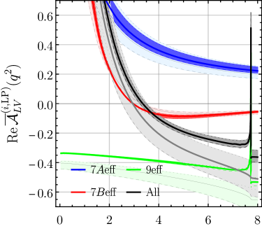
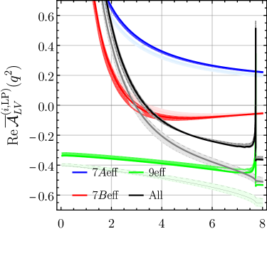
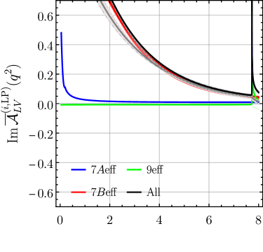
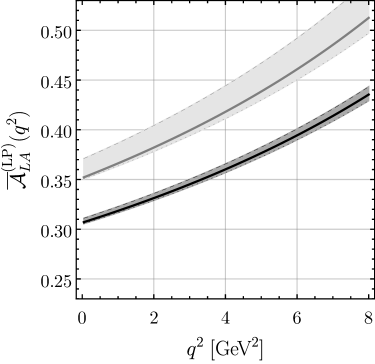
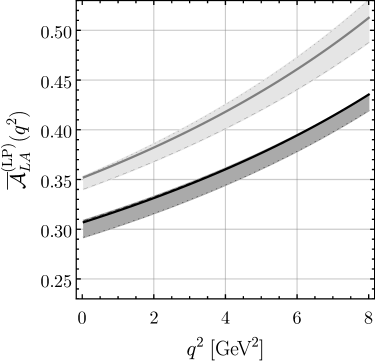
Figure 4: The $\mu_{h}$ [left] and $\mu_{hc}$ [right] dependence of the helicity amplitudes $\operatorname{Re}{\overline{\mathcal{A}}}_{LV}$ [upper], $\operatorname{Im}{\overline{\mathcal{A}}}_{LV}$ [middle] and ${\overline{\mathcal{A}}}_{LA}$ [lower] at LP. The variation of $\mu_{h}=\{2.5,\,5.0,\,10.0\}\,\text{GeV}$ and $\mu_{hc}=\{1.0,\,1.5,\,2.0\}\,\text{GeV}$ [dotted, solid, dashed] leads to the grey bands at LO QCD [lighter] and NLO QCD [darker]. The individual contributions $i=7A,7B,9$ [blue, red, green] are shown for ${\overline{\mathcal{A}}}_{LV}$.

The reduction of the dependence on $\mu_{h}=\{2.5,\,5.0,\,10.0\}\,\text{GeV}$ upon going from LO to NLO is shown in Figure 4 for ${\overline{\mathcal{A}}}_{LV}$ and ${\overline{\mathcal{A}}}_{LA}$. The NLO QCD corrections are sizeable for $V_{9}^{\text{eff}}$ and $V_{10}^{\text{eff}}$, where LO and NLO scale uncertainty bands do not overlap. These corrections have been neglected in previous predictions of $B_{q}\to\gamma\ell\bar{\ell}$. Whereas ${\overline{\mathcal{A}}}_{LA}$ is real-valued and slowly varying over $q^{2}\in[4m_{\ell}^{2},\,8.0]\,\text{GeV}^{2}$, ${\overline{\mathcal{A}}}_{LV}$ has a sizeable imaginary part already at LO QCD because of the $B$-type contribution $i=7B\text{eff}$, in contradistinction to the decays $B\to(X_{s},K,K^{*})+\ell\bar{\ell}$, where such contributions are suppressed by the small QCD-penguin coefficients. Further, $\operatorname{Re}({\overline{\mathcal{A}}}_{LV})$ is dominated for $q^{2}\lesssim 2\,\text{GeV}^{2}$ by the photon pole in $i=7A\text{eff},\,7B\text{eff}$, which interferes destructively with the $i=9\text{eff}$ contribution for $q^{2}\gtrsim 2\,\text{GeV}^{2}$ and leads to a zero crossing around $q^{2}_{0}\approx(3.0-3.5)\,\text{GeV}^{2}$. The zero crossing is responsible for the sign flip of the lepton forward-backward asymmetry $\mathcal{A}_{\text{FB}}(q^{2})$, see Section 4.2. NLO QCD corrections shift $q_{0}^{2}$ to slightly larger values and reduce the $\mu_{h}$-dependence. Moreover, in the $q^{2}$-region of the zero-crossing of the LP contribution, the total amplitude is also very sensitive to NLP corrections, see Section 4.1.2.

The dependence of ${\overline{\mathcal{A}}}_{L\chi}$ on the hard-collinear scale $\mu_{hc}$ is also shown in Figure 4, varying $\mu_{hc}=\{1.0,\,1.5,\,2.0\}\,\text{GeV}$. Also here a reduction of the scale uncertainty can be observed after including the NLO QCD corrections. Compared to the $\mu_{h}$ dependence, the residual $\mu_{hc}$ dependence at NLO is smaller in ${\overline{\mathcal{A}}}_{LV}$ and slightly larger in ${\overline{\mathcal{A}}}_{LA}$, but both scale dependencies are small compared to other theoretical uncertainties.

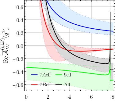
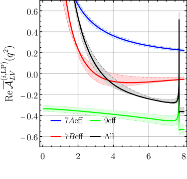
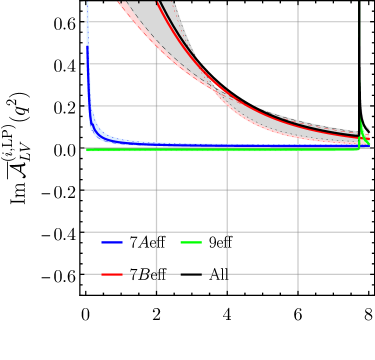
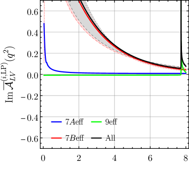
Figure 5: The $\lambda_{B_{s}}$ [left] and $\widehat{\sigma}^{(1)}_{B_{s}}$ [right] dependence of the helicity amplitudes $\operatorname{Re}{\overline{\mathcal{A}}}_{LV}$ [upper], $\operatorname{Im}{\overline{\mathcal{A}}}_{LV}$ [middle] and ${\overline{\mathcal{A}}}_{LA}$ [lower] at LP. The variation of $\lambda_{B_{s}}=(0.40\pm 0.15)\,\text{GeV}$ and $\widehat{\sigma}^{(1)}_{B_{s}}=(0.0\pm 0.7)$ [dotted, solid, dashed] leads to the grey bands. The individual contributions $i=7A,7B,9$ [blue, red, green] are also shown for ${\overline{\mathcal{A}}}_{LV}$.

The charm-quark pair threshold causes a divergence of ${\overline{\mathcal{A}}}_{LV}$ in Figure 4 at $q^{2}=4(m_{c}^{\text{PS}})^{2}\approx 7.73\,\text{GeV}^{2}$ from the two-loop matrix elements of $P_{1,2}^{c}$, which signals a breakdown of factorization and restricts us to $q^{2}\lesssim 6\,\text{GeV}^{2}$. The uncertainties due to the charm-quark mass on $\operatorname{Re}{\overline{\mathcal{A}}}_{LV}$ ($\operatorname{Im}{\overline{\mathcal{A}}}_{LV}$) for $q^{2}\lesssim 6\,\text{GeV}^{2}$ are at most $1.0\%$ ($2.0\%$) in the PS scheme. Note that the physical threshold is at $q^{2}=m_{J/\psi}^{2}>4(m_{c}^{\text{PS}})^{2}$. One might therefore be tempted to adopt the pole scheme for the charm-quark mass, in which case the partonic threshold divergence occurs closer to the physical threshold. However, we find that the uncertainty on $\operatorname{Re}{\overline{\mathcal{A}}}_{LV}$ ($\operatorname{Im}{\overline{\mathcal{A}}}_{LV}$) from $m_{c}$ for $q^{2}\lesssim 6\,\text{GeV}^{2}$ is $5.0\%$ ($5.0\%$) in the pole scheme, much larger than in the PS scheme, due to the larger uncertainty in the mass value.

The variation of the bottom-quark mass shows that for $q^{2}\lesssim 6\,\text{GeV}^{2}$ the uncertainty on $\operatorname{Re}{\overline{\mathcal{A}}}_{LV}$ ($\operatorname{Im}{\overline{\mathcal{A}}}_{LV}$) is less than $0.1\%$ ($0.3\%$) in the PS scheme and less than $0.3\%$ ($1.0\%$) in the pole scheme, and similarly for $\operatorname{Re}{\overline{\mathcal{A}}}_{LA}$.

As already mentioned, a strong dependence of ${\overline{\mathcal{A}}}_{L\chi}$ ($\chi=V,A$) on the first inverse moment $\lambda_{B_{s}}$ of the $B$-meson LCDA $\phi_{+}(\omega)$ should be expected, which is shown in Figure 5. It represents the largest uncertainty compared to the tiny $\mu_{h}$ and the $\mu_{hc}$ uncertainties, and also affects the location of the zero-crossing $q_{0}^{2}$ of $\operatorname{Re}{\overline{\mathcal{A}}}_{LV}$. To estimate the further model-dependence on the $B$-meson LCDA, we vary also the first (hatted) logarithmic moment $\widehat{\sigma}^{(1)}_{B_{s}}=(0.0\pm 0.7)$, as described in more detail in Appendix C. The uncertainty due to $\widehat{\sigma}^{(1)}_{B_{s}}$ is rather large for the contribution of $i=7B\text{eff}$, but overall small compared to the $\lambda_{B_{s}}$ uncertainty.

4.1.2 Amplitudes at NLP

The NLP corrections to the amplitudes are due to local and nonlocal $A$-type and $B$-type, as well as the local four-quark contributions in (3.42), see Section 3.2 and Figure 3.

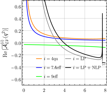
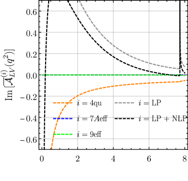
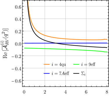
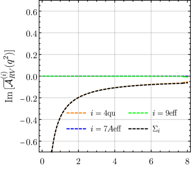
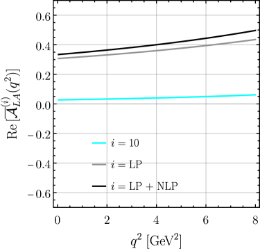
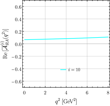
Figure 6: The local and nonlocal $A$-type NLP contributions to the real [solid] and imaginary [dashed] parts of the helicity amplitudes ${\overline{\mathcal{A}}}_{LV}$ [upper], ${\overline{\mathcal{A}}}_{RV}$ [middle] and ${\overline{\mathcal{A}}}_{hA}$ with $h=L,R$ [lower]. For comparison the LP [gray] and the total LP + NLP [black] results are also shown.

The local and nonlocal $A$-type NLP contributions to ${\overline{\mathcal{A}}}_{hV}$ ($h=L,R$) and ${\overline{\mathcal{A}}}_{LA}$ in (3.35)–(3.38) due to the semileptonic ($i=9\text{eff},\,10$) and dipole ($i=7A\text{eff}$) operators as well as the local contributions from the four-quark (4qu) operators in (3.42) are compared in Figure 6 separately to the LP results. For the non-local form factor parameterization we use the central value $r_{\text{LP}}=0.2$. It can be seen that the contributions $i=7A\text{eff},\,\text{4qu}$ have a photon pole for $q^{2}\lesssim 2\,\text{GeV}^{2}$ and that $i=\text{4qu}$ contributes an imaginary part to the left- and right-helicity amplitudes. The NLP corrections to ${\overline{\mathcal{A}}}_{LA}$ are within the expected size of a $\Lambda_{\text{QCD}}/m_{b}\sim(10-15)\%$ correction relative to LP. In the case of ${\overline{\mathcal{A}}}_{LV}$, this applies individually to the real part of $i=7A\text{eff}$ and $i=9\text{eff}$, amounting to $15\%$ and $(10-15)\%$ relative to their respective LP contributions, whereas their imaginary parts of the LP and NLP contributions are tiny ($9\text{eff}$) or vanish altogether ($7A\text{eff}$). The real and imaginary parts of the local NLP contribution $i=\text{4qu}$ turn out to be rather large, constituting $+(20-25)\%$ and $-30\%$ of the real part of the LP $i=7A\text{eff}$ contribution, which has been chosen for comparison because of a similar photon pole. The NLP corrections are most important in the $q^{2}$ region where the LP contributions cancel and give rise to the zero crossing of $\operatorname{Re}({\overline{\mathcal{A}}}_{LV})$. In fact, the location of the zero, $q^{2}_{0}\approx 4\,\text{GeV}^{2}$ is significantly shifted and the sum of these NLP corrections is sizeable compared to the LP part for $q^{2}\in[3,\,5]\,\text{GeV}^{2}$ around the zero crossing $q^{2}\in[3,\,5]\,\text{GeV}^{2}$, especially for $\operatorname{Re}({\overline{\mathcal{A}}}_{LV})$.

The right-handed helicity amplitudes ${\overline{\mathcal{A}}}_{R\chi}$ ($\chi=V,A$) are entirely NLP. ${\overline{\mathcal{A}}}_{RV}$ exhibits a zero at $q^{2}_{0}\approx 3\,\text{GeV}^{2}$ due to the interference of the $i=\text{4qu},9\text{eff}$ contributions, whereas the $i=7A\text{eff}$ part is not enhanced at $q^{2}\to 0$, see (3.38). The amplitude ${\overline{\mathcal{A}}}_{RA}$ is small.

	$m_{V}$	$\Gamma_{V}$	$f^{\parallel}_{V}$	$T_{1}^{B_{q}\to V}(0)$
$V$	$[\,\text{MeV}]$	$[\,\text{MeV}]$	$[\,\text{MeV}]$
$\phi(1020)$	$1019.461(16)$	$4.249(13)$	$233(4)$	$0.309(27)$
$\phi(1680)$	$1680(20)$	$150(50)$	—	—
$\phi(2170)$	$2170(15)$	$104(20)$	—	—
$\rho^{0}(770)$	$775.26(25)$	$147.8(9)$	$213(5)$	$0.272(26)$
$\omega(782)$	$782.65(12)$	$8.49(8)$	$197(8)$	$0.251(31)$
$\omega(1420)$	$1410(60)$	$290(190)$	—	—
$\rho(1450)$	$1465(25)$	$400(60)$	—	—

Table 2: Numerical input values for the parameters of the resonances entering the $b\to s$ and $b\to d$ transitions. Masses and decay widths are from [47] and decay constants and form factors from [45], with the $q^{2}$ dependence of $T_{1}^{B_{q}\to V}$ in the simplified series expansion (SSE) in Table 14 from light-cone sum rules only.

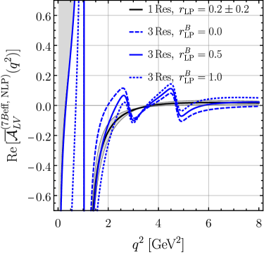
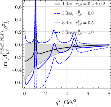
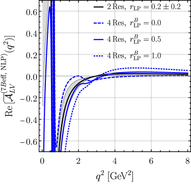
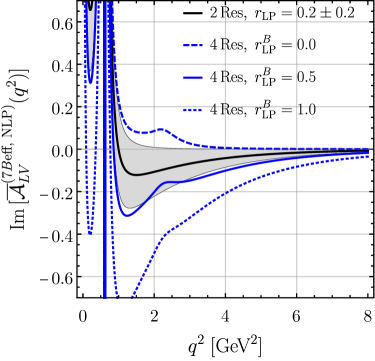
Figure 7: The real [left] and imaginary [right] parts of the NLP local + nonlocal $7B\text{eff}$-type contributions $i=7B\text{eff}$ to ${\overline{\mathcal{A}}}_{LV}$ for $q=s$ [upper] and $q=d$ [lower]. The default 1(2)-Res model for $r_{\text{LP}}=0.2\pm 0.2$ [grey band] is compared with the 3(4)-Res model for $r^{B}_{\text{LP}}=\{0.0,\,0.5,\,1.0\}$ [blue dashed, solid, dotted].

The $B$-type NLP contributions ($i=7B\text{eff}$) enter only in ${\overline{\mathcal{A}}}_{LV}$. The nonlocal form factors are modelled according to Section 3.4 with parameters listed in Table 2. The lowest resonances affect the very-low $q^{2}$ region $q^{2}\lesssim 1\,\,\text{GeV}$: $\phi(1020)$ for $q=s$, and $\rho^{0}(770)$ and $\omega(782)$ for $q=d$. We include these lowest resonances in our default model (“1(2) Res”) in both $A$- and $B$-type contributions. Further we describe the continuum part of the nonlocal NLP $B$-type contribution by the fraction $r_{\text{LP}}=0.2\pm 0.2$ of the LP $B$-type amplitude (3.15), omitting NLO QCD corrections. The positive central value of $r_{\text{LP}}$ implies destructive interference with the LP contribution, see (3.57), in agreement with sum rule calculations of the corresponding $A$-type form factor [24]. The resulting $B$-type NLP contributions to the helicity amplitudes are shown in Figure 7 as solid black line and grey band.

The $B$-type contribution needs the form factor in the time-like region. In order to investigate the impact of higher-mass resonances on this form factor, we define an alternative model (“3(4) Res”), which includes the next two resonances listed in Table 2 in the sum over $V$ in (3.57). We assume the unknown decay constants and form factors of the higher $\phi$, $\rho$ and $\omega$ resonances to be a fraction

$$r^{q}_{fT}\equiv\Big{(}f_{V^{\prime}}T_{1}^{B_{q}\to V^{\prime}}\Big{)}\Big{/}\Big{(}f_{V}T_{1}^{B_{q}\to V}\Big{)}\hskip 56.9055pt(q=d,s)$$ (4.6)

of those of the lowest ones and use the same value $r^{q}_{fT}=0.3$ for all higher resonances $V^{\prime}>V$. Since the higher resonances lie in the range of $q^{2}$, where we might expect the continuum contribution calculated in factorization to already be dual to the contribution from the relatively broad resonances, the value of $r_{\text{LP}}$ should be increased (implying a smaller continuum part in the sum of LP and NLP according to (3.57)). Hence, we introduce separate parameters $r_{\text{LP}}^{A}$ and $r_{\text{LP}}^{B}$, where the first is always kept at $r_{\text{LP}}^{A}=0.2\pm 0.2$, but the second should depart from this value in the “3(4) Res” model, at least for $q=s$, where the effect of resonances is more pronounced.

In Figure 7 the default model is compared to the one including the higher resonances. In the case $q=s$ (upper plots), the higher $\phi$ resonances are clearly visible despite their large widths of about $(100-150)\,\text{MeV}$. The “3-Res” model is shown for three different values of $r_{\text{LP}}^{B}$ and oscillates around the default 1-Res model for the real part independently of the choice of $r_{\text{LP}}$. On the other hand, the imaginary part is very sensitive to this choice. For $r_{\text{LP}}^{B}\approx 0.5$ the local effects of the resonances would be included globally in the 1-Res model with $r_{\text{LP}}^{B}=0.2$, in agreement with the qualitative expectation above. In the case of $q=d$ (lower plots) the effect of the excited resonances $\rho(1450)$ and $\omega(1420)$ is much smaller in ${\overline{\mathcal{A}}}_{LV}$, such that local duality above $q^{2}\gtrsim 2.0\,\text{GeV}^{2}$ works better compared to $q=s$. Also we see that with $r_{\text{LP}}^{B}\approx 0.3$ the 4-Res description is close to the 2-Res one, again in agreement with expectations.

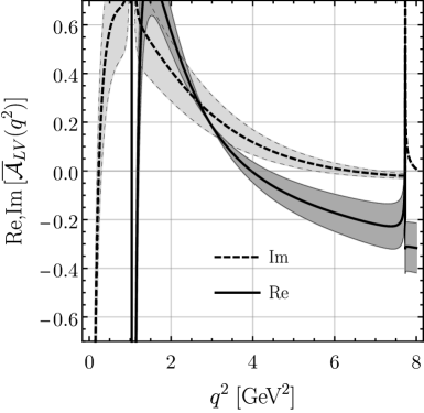
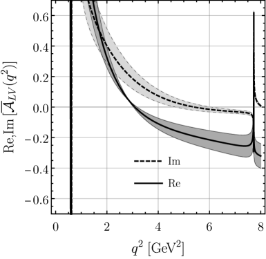
Figure 8: The real [solid, darker] and imaginary [dashed, lighter] part of the combined LP and NLP result for ${\overline{\mathcal{A}}}_{LV}$ in the default 1- and 2-Res model for $q=s$ [left] and $q=d$ [right], respectively. The grey band shows the variation $r_{\text{LP}}=0.2\pm 0.2$.

The final result of ${\overline{\mathcal{A}}}_{LV}$, including all contributions (LP and NLP, $A$-type and $B$-type), is shown in Figure 8 for the default 1(2)-Res model of the NLP nonlocal $B$-type contributions. The variation $r_{\text{LP}}=0.2\pm 0.2$ gives rise to the bands for the real and imaginary parts. The zero crossing of the real part for $q=s$ is shifted to $q_{0}^{2}\approx 4\,\text{GeV}^{2}$ when compared to the LP result of ${\overline{\mathcal{A}}}_{LV}$ in Figure 4. For $q=d$, the zero-crossing occurs at the lower value $q_{0}^{2}\approx 2.5\,\text{GeV}^{2}$.

4.2 $B_{q}\to\gamma\ell\bar{\ell}$ observables

From the amplitude (4.1) we obtain the two-fold ${\overline{B}}_{q}\to\gamma\ell\bar{\ell}$ decay-rate distribution

$$\frac{d^{2}{\overline{\Gamma}}}{dq^{2}\,d\!\cos\theta_{\ell}}\Big{|}_{|\text{SD}|^{2}} ={\overline{a}}(q^{2})+{\overline{b}}(q^{2})\cos\theta_{\ell}+{\overline{c}}(q^{2})\cos^{2}\!\theta_{\ell}$$ (4.7)

in terms of the kinematic variables $q^{2}\in[4m_{\ell}^{2},\,m_{B_{q}}^{2}]$ and $\cos\theta_{\ell}\in[-1,\,1]$, where $\theta_{\ell}$ is the angle between the ${\overline{B}}_{q}$-meson direction and the lepton momentum in the dilepton center-of-mass frame. The $q^{2}$-dependent angular coefficients are expressed in terms of the transversity amplitudes as follows:

$${\overline{a}} =\Gamma_{0}\sqrt{\lambda}^{3}q^{2}\beta_{\ell}\times\Big{[}(2-\beta_{\ell}^{2})\left(|{\overline{\mathcal{A}}}_{\parallel V}|^{2}+|{\overline{\mathcal{A}}}_{\perp V}|^{2}\right)+\beta_{\ell}^{2}\left(|{\overline{\mathcal{A}}}_{\parallel A}|^{2}+|{\overline{\mathcal{A}}}_{\perp A}|^{2}\right)\Big{]},$$ (4.8)

$${\overline{b}} =\Gamma_{0}\sqrt{\lambda}^{3}q^{2}\beta_{\ell}\times 4\,\beta_{\ell}\,\text{Re}\Big{[}{\overline{\mathcal{A}}}_{\parallel V}{\overline{\mathcal{A}}}_{\perp A}^{\ast}+{\overline{\mathcal{A}}}_{\parallel A}{\overline{\mathcal{A}}}_{\perp V}^{\ast}\Big{]},$$ (4.9)

$${\overline{c}} =\Gamma_{0}\sqrt{\lambda}^{3}q^{2}\beta_{\ell}\times\beta_{\ell}^{2}\Big{[}|{\overline{\mathcal{A}}}_{\parallel V}|^{2}+|{\overline{\mathcal{A}}}_{\perp V}|^{2}+|{\overline{\mathcal{A}}}_{\parallel A}|^{2}+|{\overline{\mathcal{A}}}_{\perp A}|^{2}\Big{]},$$ (4.10)

and

$$\Gamma_{0} \equiv\frac{\alpha_{\text{em}}^{3}|\mathcal{N}_{\text{ew}}|^{2}}{2^{11}\pi^{4}m_{B_{q}}^{5}}, \sqrt{\lambda} \equiv m_{B_{q}}^{2}-q^{2}, \beta_{\ell} \equiv\sqrt{1-\frac{4m_{\ell}^{2}}{q^{2}}}.$$ (4.11)

Eq. (4.7) refers to the square of the so-called structure-dependent (SD) amplitude. We provide the lepton-mass suppressed parts of the double-differential width due to the FSR amplitude of $P_{10}$ and its interferences with the SD amplitude in Appendix B. The differential decay width and the normalized lepton forward-backward asymmetry are

$$\frac{d{\overline{\Gamma}}}{dq^{2}} =2\left[{\overline{a}}(q^{2})+\frac{{\overline{c}}(q^{2})}{3}\right]+\ldots, {\overline{A}}_{\text{FB}}(q^{2}) =\frac{{\overline{b}}(q^{2})}{d{\overline{\Gamma}}/dq^{2}}+\ldots,$$ (4.12)

where the dots denote lepton-mass suppressed terms from the FSR contribution. The angular observables ${\overline{a}}(q^{2})$ and ${\overline{c}}(q^{2})$ differ only by lepton-mass effects, such that their difference

$${\overline{a}}(q^{2})-{\overline{c}}(q^{2}) \propto 2(1-\beta_{\ell}^{2})\left(|{\overline{\mathcal{A}}}_{\parallel V}|^{2}+|{\overline{\mathcal{A}}}_{\perp V}|^{2}\right)\propto\frac{m_{\ell}^{2}}{q^{2}}\left(|{\overline{\mathcal{A}}}_{\parallel V}|^{2}+|{\overline{\mathcal{A}}}_{\perp V}|^{2}\right)$$ (4.13)

is lepton-mass suppressed. The lepton-mass suppression renders the experimental measurement of these parts of the two-fold differential decay width challenging. Moreover, the lepton-mass suppressed FSR contributions in Appendix B cannot be disentangled from them and introduce a dependence on $C_{10}$, which is absent in ${\overline{a}}(q^{2})-{\overline{c}}(q^{2})$. Further, the FSR contribution introduces a nonanalytic $\cos\theta_{\ell}$ dependence as can be seen in (B.6) and (B.7). In consequence there are the two main observables, $d{\overline{\Gamma}}/dq^{2}$ and ${\overline{A}}_{\text{FB}}(q^{2})$, in the part of the phase space where $4m_{\ell}^{2}\ll q^{2}$.

The two-fold decay-rate distribution

$$\frac{d^{2}\Gamma}{dq^{2}\,d\!\cos\theta_{\ell}}\Big{|}_{|\text{SD}|^{2}} =a(q^{2})-b(q^{2})\cos\theta_{\ell}+c(q^{2})\cos^{2}\!\theta_{\ell}$$ (4.14)

for the CP-conjugated decay $B_{q}\to\gamma\ell\bar{\ell}$ is given by the quantities $a$, $b$ and $c$ without bars, which are obtained from (4.8)–(4.10) by using the CP-conjugated transversity amplitudes $\mathcal{A}_{\perp\chi}$ and $\mathcal{A}_{\parallel\chi}$ ($\chi=V,A$). The CP-transformation properties (4.4) of $\mathcal{A}_{\perp\chi}$ imply a minus sign in front of $b(q^{2})$ in correspondence with other $B\to V\ell\bar{\ell}$ decays ($V=K^{*},\phi,\ldots$) [65].

The combination of the two-fold decay-rate distributions of the decay (4.7) and the CP-conjugated decay (4.14) allows for two CP-averaged and two CP-asymmetric observables. We consider the CP-averaged rate and the normalized lepton-forward-backward asymmetry as well as the CP rate asymmetry, defined by

$$\frac{d\mathcal{B}}{dq^{2}} =\frac{\tau_{B_{q}}}{2}\frac{d[{\overline{\Gamma}}+\Gamma]}{dq^{2}}, \mathcal{A}_{\text{FB}}(q^{2}) =\frac{[{\overline{b}}+b](q^{2})}{d[{\overline{\Gamma}}+\Gamma]/dq^{2}}, \mathcal{A}_{\text{CP}}(q^{2}) =\frac{d[{\overline{\Gamma}}-\Gamma]/dq^{2}}{d[{\overline{\Gamma}}+\Gamma]/dq^{2}}.$$ (4.15)

We do not study the CP-asymmetry of the normalized lepton-forward-backward asymmetry defined as $\mathcal{A}^{\text{CP}}_{\text{FB}}=[{\overline{b}}-b](q^{2})/(d[\Gamma+{\overline{\Gamma}}]/dq^{2})$. We note that an untagged sample actually depends on the CP asymmetry of the lepton forward-backward asymmetry $\mathcal{A}^{\text{CP}}_{\text{FB}}(q^{2})\propto d^{2}[{\overline{\Gamma}}+\Gamma]\propto[{\overline{b}}-b](q^{2})$. On the other hand the measurement of the lepton forward-backward asymmetry $\mathcal{A}_{\text{FB}}(q^{2})\propto d^{2}[{\overline{\Gamma}}-\Gamma]\propto[{\overline{b}}+b](q^{2})$ requires tagging.

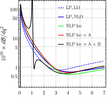
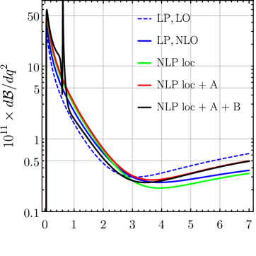
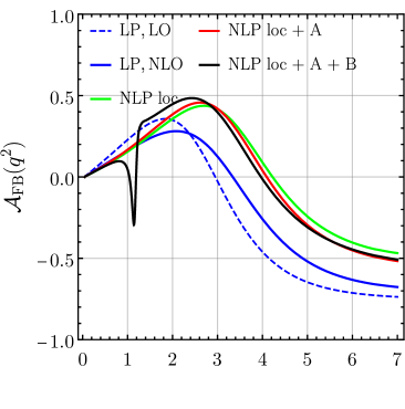
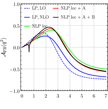
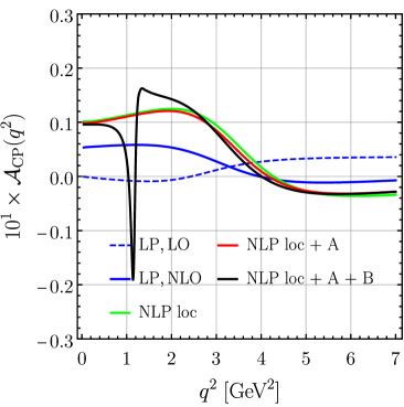
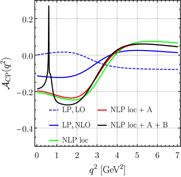
Figure 9: The $d\mathcal{B}/dq^{2}$ [upper], $\mathcal{A}_{\text{FB}}(q^{2})$ [middle] and $\mathcal{A}_{\text{CP}}(q^{2})$ [lower] distributions for $B_{s}\to\gamma\mu\bar{\mu}$ [left] and $B_{d}\to\gamma\mu\bar{\mu}$ [right] when adding successively various contributions: only LP [blue] at LO QCD [dashed] and NLO QCD [solid]; + local NLP corrections [green]; + nonlocal $A$-type [red]; + nonlocal $B$-type with lowest resonances [black] NLP corrections. The parameter $r_{\text{LP}}=0.2$.

The $q^{2}$ dependencies of the branching fraction $d\mathcal{B}/dq^{2}$, $\mathcal{A}_{\text{FB}}(q^{2})$ and $\mathcal{A}_{\text{CP}}(q^{2})$ for $B_{s}\to\gamma\mu\bar{\mu}$ and $B_{d}\to\gamma\mu\bar{\mu}$ are shown in Figure 9 when including successively the various higher-order QCD and NLP corrections discussed in Section 3. We recall that the calculation is valid in the “low-$q^{2}$” region $q^{2}\lesssim 6\,\text{GeV}^{2}$ or equivalently $E_{\gamma}\gtrsim 2.1\,\text{GeV}$ ($y\gtrsim 0.8$). In the figure, the NLP corrections have been separated into 1) purely local (“loc”), 2) nonlocal $A$-type (“A”) as given in (3.56) and 3) nonlocal $B$-type (“B”) as given in (3.57). At LP, the NLO QCD corrections – see “LP, LO” vs. “LP, NLO” – decrease (increase) $d\mathcal{B}/dq^{2}$ for $q^{2}\gtrsim 3.0\,\text{GeV}^{2}$ ($q^{2}\lesssim 3.0\,\text{GeV}^{2}$) and shift the position of the zero-crossing of $\mathcal{A}_{\text{FB}}(q^{2})$ by about $\Delta q^{2}_{0}\approx+0.5\,\text{GeV}^{2}$ towards higher values. Further, the NLO QCD corrections substantially change the CP asymmetry $\mathcal{A}_{\text{CP}}(q^{2})$. The CP asymmetry is always tiny for $q=s$, because it is suppressed by the Cabibbo angle, but for $q=d$ it can be reach $-10\%$ locally below the zero-crossing at $q^{2}\gtrsim 3.5\,\text{GeV}^{2}$.

The local NLP corrections lead to a decrease of about $(15-20)\%$ of $d\mathcal{B}/dq^{2}$ for $q^{2}\gtrsim 3.0\,\text{GeV}^{2}$, i.e. in the region where the individual LP contributions $i=7A\text{eff},\,7B\text{eff},\,9\text{eff}$ cancel, and give a large shift $\Delta q^{2}_{0}\approx+0.8\,\text{GeV}^{2}$ to the zero of the $\mathcal{A}_{\text{FB}}(q^{2})$. The inclusion of $A$-type nonlocal corrections (“NLP loc$\,+\,$A”) almost cancels the effect of “NLP loc” in $d\mathcal{B}/dq^{2}$, but not so in $\mathcal{A}_{\text{FB}}(q^{2})$ and $\mathcal{A}_{\text{CP}}(q^{2})$ for the chosen input $r^{q}_{fT}=0.3$ and $r_{\text{LP}}=0.2$, leaving $\mathcal{A}_{\text{CP}}(q^{2})$ for $q=d$ at about $-20\%$ at very low $q^{2}$ and $+5\%$ at higher $q^{2}$. The NLP nonlocal $B$-type corrections for the default model with only lowest resonances affects only the very-low $q^{2}$ region, with strong impact from the $\phi(1020)$ on $d\mathcal{B}/dq^{2}$ for $q=s$. The lowest resonances also affect the $\mathcal{A}_{\text{FB}}(q^{2})$ and $\mathcal{A}_{\text{CP}}(q^{2})$ locally in $q^{2}$. In total, the zero-crossing $q_{0}^{2}$ is significantly increased by NLP contributions compared to “LP, NLO”. The difference in $q_{0}^{2}$ between $B_{s}$ and $B_{d}$ decays of about $0.5\,\text{GeV}^{2}$ is due to a different value of $\lambda_{B_{q}}$, but also non-negligible contributions $\propto\lambda_{u}^{(q)}$ for $q=d$.

At very low $q^{2}$ the distributions shown in Figure 9 are strongly affected locally by the resonances from the $B$-type contributions, and therefore prone to the uncertainty in modelling the corresponding form factor. In the spirit of global parton-hadron duality, we investigate whether such effects become averaged once integrated over sufficiently large bins in $q^{2}$. The $q^{2}$ bins are chosen in the low-$q^{2}$ region, with upper bin boundary $q^{2}_{\text{max}}=6\,\text{GeV}^{2}$ to avoid large impacts of charmonium resonances. The lower bin boundaries are chosen as $q^{2}_{\text{min}}=\{4m_{\mu}^{2},\,1.0,\,2.0,\,3.0,\,4.0\}\,\text{GeV}^{2}$, excluding $q^{2}_{\text{min}}=1.0\,\text{GeV}^{2}$ for $q=s$ because it is at the center of the $\phi(1020)$ peak region. The results for $\mathcal{B}(B_{s}\to\gamma\mu\bar{\mu})$ and $\mathcal{B}(B_{d}\to\gamma\mu\bar{\mu})$ are listed in Table 3 for the same approximations of the various curves as in Figure 9.

$q^{2}$ bin	LP		NLP			uncertainty of “NLP all”
$[\,\text{GeV}^{2}]$	LO	NLO	loc	loc$\,+\,$A	all	$\mu_{h,hc}$	$\lambda_{B_{q}},\,\widehat{\sigma}^{(q)}_{B_{1}}$	$r_{\text{LP}}$	total
$B_{s}\to\gamma\mu\bar{\mu}$
$[4m_{\mu}^{2},\,6.0]$	2.32	2.96	3.81	4.03	12.43	${}_{-0.56}^{+0.11}$	${}_{-1.42}^{+3.56}$	${}_{-1.19}^{+1.39}$	${}_{-1.93}^{+3.83}$
$[2.0,\,6.0]$	0.40	0.34	0.31	0.36	0.30	${}_{-0.04}^{+0.01}$	${}_{-0.08}^{+0.21}$	${}_{-0.11}^{+0.14}$	${}_{-0.14}^{+0.25}$
$[3.0,\,6.0]$	0.30	0.22	0.19	0.22	0.21	${}_{-0.03}^{+0.01}$	${}_{-0.07}^{+0.18}$	${}_{-0.08}^{+0.10}$	${}_{-0.10}^{+0.20}$
$[4.0,\,6.0]$	0.22	0.15	0.12	0.15	0.15	${}_{-0.02}^{+0.01}$	${}_{-0.05}^{+0.14}$	${}_{-0.05}^{+0.07}$	${}_{-0.08}^{+0.16}$
$[4m_{\mu}^{2},\,8.64]$	2.77	3.24	4.05	4.34	12.74	${}_{-0.60}^{+0.14}$	${}_{-1.50}^{+3.85}$	${}_{-1.31}^{+1.54}$	${}_{-2.08}^{+4.15}$
$B_{d}\to\gamma\mu\bar{\mu}$
$[4m_{\mu}^{2},\,6.0]$	8.77	11.31	14.07	15.54	18.43	${}_{-1.17}^{+0.43}$	${}_{-5.67}^{+17.46}$	${}_{-4.33}^{+5.08}$	${}_{-7.23}^{+18.19}$
$[1.0,\,6.0]$	2.39	2.52	2.60	3.01	2.34	${}_{-0.28}^{+0.13}$	${}_{-0.69}^{+1.71}$	${}_{-0.77}^{+0.97}$	${}_{-1.07}^{+1.97}$
$[2.0,\,6.0]$	1.52	1.25	1.13	1.43	1.29	${}_{-0.16}^{+0.06}$	${}_{-0.39}^{+1.13}$	${}_{-0.43}^{+0.56}$	${}_{-0.60}^{+1.26}$
$[3.0,\,6.0]$	1.17	0.83	0.71	0.96	0.92	${}_{-0.11}^{+0.06}$	${}_{-0.32}^{+1.00}$	${}_{-0.32}^{+0.42}$	${}_{-0.47}^{+1.09}$
$[4.0,\,6.0]$	0.86	0.56	0.49	0.68	0.67	${}_{-0.08}^{+0.05}$	${}_{-0.25}^{+0.76}$	${}_{-0.24}^{+0.31}$	${}_{-0.35}^{+0.83}$
$[4m_{\mu}^{2},\,8.64]$	10.53	12.38	15.03	16.98	19.85	${}_{-1.33}^{+0.33}$	${}_{-6.07}^{+19.10}$	${}_{-4.85}^{+5.74}$	${}_{-7.88}^{+19.95}$

Table 3: The $q^{2}$-integrated branching fractions $10^{9}\times\mathcal{B}(B_{s}\to\gamma\mu\bar{\mu})$ and $10^{11}\times\mathcal{B}(B_{d}\to\gamma\mu\bar{\mu})$ in four / five bins in the various approximations shown in Figure 9. “NLP all” corresponds to “NLP loc + A + B” in Figure 9. The last four columns list the uncertainties due to 1) renormalization scale uncertainties, 2) $B$-meson LCDA parameters and 3) the continuum fraction $r_{\text{LP}}$ as well as “total” when adding them in quadrature.

The block of the first three corrections in Table 3, “LP, LO” through “NLP, loc”, are found within systematic approximations and assumptions, and can be considered as model-independent. Omitting for a moment the nonlocal $B$-type contributions and comparing “NLP loc$\,+\,$A” in the first two bins of $\mathcal{B}(B_{s}\to\gamma\mu\bar{\mu})$ shows that the photon pole at $q^{2}\to 4m_{\mu}^{2}$ in the bin $q^{2}\in[4m_{\mu}^{2},\,2.0\,\text{GeV}^{2}]$ contributes almost 90% of the rate. In this approximation the rate is of the order $4\cdot 10^{-9}$, comparable to the branching fraction $\mathcal{B}(B_{s}\to\mu\bar{\mu})$ of the non-radiative mode. When adding the nonlocal $B$-type contributions, however, the $\phi(1020)$ contribution dominates over these “short-distance” corrections and enhances the rate by a factor of three to $12\cdot 10^{-9}$, see “NLP all”, and is responsible for about 70% of the signal in the bin $[4m_{\mu}^{2},\,6.0\,\text{GeV}^{2}]$. The photon pole constitutes also about 80% of the rate of $\mathcal{B}(B_{d}\to\gamma\mu\bar{\mu})$ in $q^{2}\in[4m_{\mu}^{2},\,6.0\,\text{GeV}^{2}]$ when omitting the nonlocal $B$-type contributions due to the $\rho$ and $\omega$ resonances, which however have only a small impact compared to the $\phi$ in $\mathcal{B}(B_{s}\to\gamma\mu\bar{\mu})$, as expected from the discussion of duality violation in Section 3.3. They enhance the rate by a factor $1.2$ to about $1.8\cdot 10^{-10}$, which is comparable to the SM prediction of $\mathcal{B}(B_{d}\to\mu\mu)\approx 1\cdot 10^{-10}$. The comparison of the first bin $[4m_{\mu}^{2},\,6.0\,\text{GeV}^{2}]$ to the second bin shows that the branching fractions are reduced by a factor of about $40$ and $8$ for $q=s$ and $q=d$, respectively, once the photon pole contribution is excluded, making them an order of magnitude smaller than for the corresponding non-radiative rare decays, $B_{q}\to\mu\bar{\mu}$. Note, however, that for $\ell=e$ the $B_{q}\to e\bar{e}$ rates are strongly helicity suppressed by $(m_{e}/m_{\mu})^{2}$, whereas the rates of $B_{q}\to\gamma e\bar{e}$ are identical to $B_{q}\to\gamma\mu\bar{\mu}$ in the SM up to phase-space effects for very low $q^{2}$.

Comparison of the value $\mathcal{B}(B_{s}\to\gamma\mu\bar{\mu})=(8.4\pm 1.3)\cdot 10^{-9}$ in the $q^{2}$ bin $[4m_{\mu}^{2},\,8.64\,\text{GeV}^{2}]$ given in [10] with Table 3 shows that our prediction is about a factor 1.5 larger and within the given errors there is some tension. Here we used the QCD factorization approach to compute the $A$- and $B$-type contributions, allowing us also to include at LP the NLO QCD corrections, contrary to [10]. In addition, we include in our model of the nonlocal NLP $A$- and $B$-type contributions also a continuum contribution. On the other hand we do not include a model for charmonium resonances (but rather stay away from them by restricting $q^{2}\lesssim 6$ GeV²), which could be responsible for some differences when $q^{2}$ approaches $8\,\text{GeV}^{2}$. Similar comments apply to [11] who predict $\mathcal{B}(B_{s}\to\gamma\mu\bar{\mu})=7.79\cdot 10^{-9}$ in the bin $q^{2}\in[4m_{\mu}^{2},\,6.0\,\text{GeV}^{2}]$ and $\mathcal{B}(B_{d}\to\gamma\mu\bar{\mu})=(1.02\pm 0.16)\cdot 10^{-11}$ in the bin $q^{2}\in[1.0,\,6.0]\,\text{GeV}^{2}$, roughly a factor of 1.6 and 2.3, respectively, smaller than our results in Table 3. We attribute these differences to the difference between the QCD factorization computation of the $B\to\gamma^{*}$ form factors and the more model-dependent approaches used in [10, 11], and differences in the numerical values of the $T_{1}^{B_{q}\to V}$ form factors in the parameterization of the nonlocal NLP $B$-type contribution relative to [11].

We calculate the theoretical uncertainties from 1) scale variation, 2) $B$-meson LCDA parameters and 3) the modelling of the nonlocal $A$- and $B$-type contributions, as discussed for the amplitudes in Section 4.1. They are listed for the best approximation “NLP, all” in Table 3 and shown in Figure 10 for the $q^{2}$- distributions $d\mathcal{B}/dq^{2}$, $\mathcal{A}_{\text{FB}}(q^{2})$ and $\mathcal{A}_{\text{CP}}(q^{2})$. The default 1(2)-Res model is used and the uncertainties are added successively in quadrature.

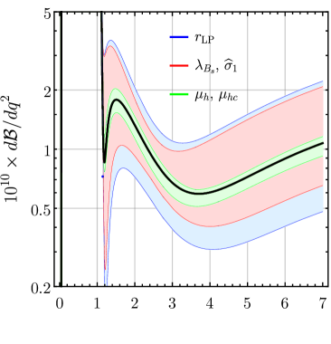
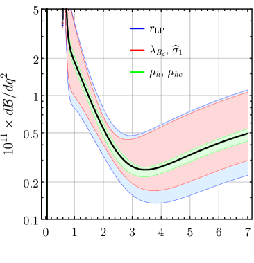
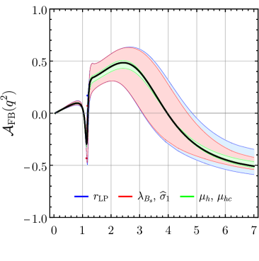
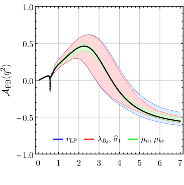
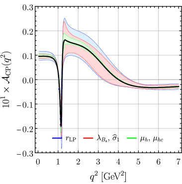
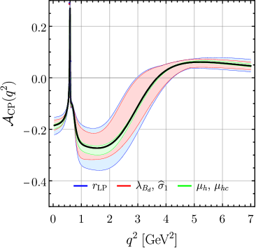
Figure 10: Uncertainty budget for $d\mathcal{B}/dq^{2}$ [upper], $\mathcal{A}_{\text{FB}}(q^{2})$ [middle] and $\mathcal{A}_{\text{CP}}(q^{2})$ [lower] for $q=s$ [left] and $q=d$ [right] when adding successively in quadrature the uncertainties due to renormalization scales ($\mu_{h,hc}$) [green], $B$-meson LCDA parameters ($\lambda_{B_{q}},\,\widehat{\sigma}^{(1)}_{B_{q}}$) [red] and the continuum fraction ($r_{\text{LP}}$) [blue].

The largest uncertainty is due to the LCDA parameters, amounting to about ${}^{+70}_{-30}\,$% for $B_{s}\to\gamma\mu\bar{\mu}$ in the bin $q^{2}\in[2.0,\,6.0]\,\text{GeV}^{2}$ (see Table 3), in particular the first inverse moment of the $B$-meson LCDA, $\lambda_{B_{q}}$, since roughly the LP is proportional to $1/\lambda_{B_{q}}$. It is even larger for $B_{d}\to\gamma\mu\bar{\mu}$ in that $q^{2}$ bin, because here the relative variation of $\lambda_{B_{d}}=(350\pm 150)\,\text{MeV}$ is larger and the minimal value in the variation is $200\,\text{MeV}$ to be compared to $\lambda_{B_{s}}=(400\pm 150)\,\text{MeV}$. The variation $r_{\text{LP}}=0.2\pm 0.2$ of the continuum fraction in the form factors model for the nonlocal $A$- and $B$-type contributions contributes another $\pm(35-45)\,$% to the uncertainty when going to $q_{\text{min}}^{2}\gtrsim 2.0\,\text{GeV}^{2}$, beyond the region of the lowest resonances. The large uncertainty of the power-suppressed contributions does not come as a surprise given that the continuum is modelled as a fraction of up to 40% of the LP amplitude.

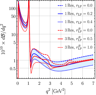
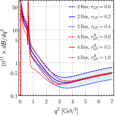
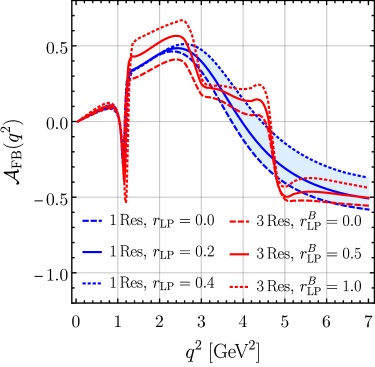
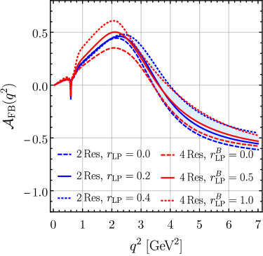
Figure 11: Comparison of the 1(2)-Res model with a continuum of $r_{\text{LP}}=0.2\pm 0.2$ [blue] with the 3(4)-Res model for different values $r_{\text{LP}}^{B}$ with fixed $r_{\text{LP}}^{A}=0.2$ [red] for $d\mathcal{B}/dq^{2}$ [upper] and $\mathcal{A}_{\text{FB}}(q^{2})$ [lower] in $B_{s}\to\gamma\mu\bar{\mu}$ [left] and $B_{d}\to\gamma\mu\bar{\mu}$ [right].

The nonlocal $B$-type corrections affect the $q^{2}$-differential distributions particularly in the very-low $q^{2}$ domain as shown at the amplitude level in Figure 7. There the default 1(2)-Res model was compared to the 3(4)-Res model for various values of the continuum fraction $r_{\text{LP}}^{B}$. This comparison is extended to the observables $d\mathcal{B}/dq^{2}$ and $\mathcal{A}_{\text{FB}}(q^{2})$ in Figure 11. The 1(2)-Res model with a continuum parameter $r_{\text{LP}}^{A}=r_{\text{LP}}^{B}=0.2\pm 0.2$ (blue) is compared to the 3(4)-Res model for various values $r_{\text{LP}}^{B}$ and fixed $r_{\text{LP}}^{A}=0.2$ (red). The variation of $r_{\text{LP}}$ in the 1-Res model spans a band that includes in the case of $d\mathcal{B}[B_{s}\to\gamma\mu\bar{\mu}]/dq^{2}$ the effect of $\phi(1680)$ in the 3-Res model for values $r_{\text{LP}}^{B}\approx 0.5$ and for the $\phi(2170)$ even for all values $r_{\text{LP}}^{B}\approx[0.0,\,1.0]$. For $\mathcal{A}_{\text{FB}}(q^{2})$ the higher resonances are locally not completely covered by this band, but oscillate around it, such that suitable binning would indeed average out the resonances. The comparison of the 2-Res with the 4-Res model in $B_{d}\to\gamma\mu\bar{\mu}$ shows a small impact of the higher resonances in all distributions as expected from the discussion of the corresponding amplitudes.

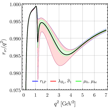
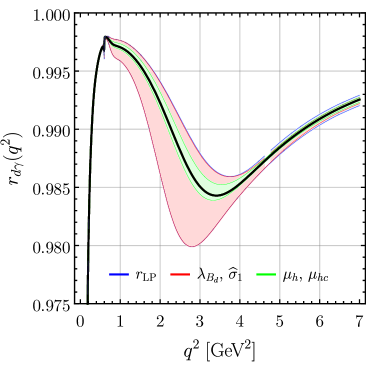
Figure 12: The ratio $r_{q\gamma}$ for $B_{s}\to\gamma\ell\bar{\ell}$ [left] and $B_{d}\to\gamma\ell\bar{\ell}$ [right] with uncertainty budget as in Figure 10.

The ratios of observables with different lepton flavours provide interesting tests of lepton-flavour universality. The deviations from unity are tiny in the SM, and hadronic uncertainties cancel to large extent. Here we briefly discuss the ratio

$$r_{q\gamma}(q^{2}) =\frac{d\mathcal{B}[B_{q}\to\gamma\mu\bar{\mu}]/dq^{2}}{d\mathcal{B}[B_{q}\to\gamma e\bar{e}]/dq^{2}} (q =d,s).$$ (4.16)

As shown in Figure 12, these ratios take values between $(0.98-1.00)$ for both $q=s,d$, except for $q^{2}\lesssim 0.4\,\text{GeV}^{2}$. Within the framework of our calculation, lepton-mass dependence arises only from $\beta_{\ell}$ through the phase-space measure, not from the amplitudes themselves. In Table 4 we give the ratio

$$R_{q\gamma} ={\displaystyle\int_{q^{2}_{\text{min}}}^{q^{2}_{\text{max}}}dq^{2}\frac{d\mathcal{B}[B_{q}\to\gamma\mu\bar{\mu}]}{dq^{2}}}\Bigg{/}{\displaystyle\int_{q^{2}_{\text{min}}}^{q^{2}_{\text{max}}}dq^{2}\frac{d\mathcal{B}[B_{q}\to\gamma e\bar{e}]}{dq^{2}}} (q =d,s)$$ (4.17)

for selected bins in $q^{2}$. $R_{q\gamma}$ is always very close to unity except when $q^{2}_{\text{min}}$ is below $1\,\text{GeV}^{2}$. The considered sources of uncertainties cancel to very high degree, and in view of the remaining tiny errors one should keep in mind that further not included higher order QCD and QED as well as NLP corrections can contribute at this level.

$q^{2}$ bin	$B_{s}\to\gamma\ell\bar{\ell}$		$B_{d}\to\gamma\ell\bar{\ell}$
$[\,\text{GeV}^{2}]$	cen	total	cen	total
$[4m_{\mu}^{2},\,6.0]$	0.9716	${}_{-0.0137}^{+0.0081}$	0.9263	${}_{-0.0093}^{+0.0046}$
$[1.0,\,6.0]$	—	—	0.9913	${}_{-0.0028}^{+0.0013}$
$[2.0,\,6.0]$	0.9883	${}_{-0.0021}^{+0.0012}$	0.9878	${}_{-0.0022}^{+0.0011}$
$[3.0,\,6.0]$	0.9875	${}_{-0.0009}^{+0.0007}$	0.9874	${}_{-0.0009}^{+0.0005}$
$[4.0,\,6.0]$	0.9883	${}_{-0.0006}^{+0.0005}$	0.9885	${}_{-0.0006}^{+0.0004}$
$[4m_{\mu}^{2},\,8.64]$	0.9721	${}_{-0.0130}^{+0.0077}$	0.9308	${}_{-0.0078}^{+0.0037}$

Table 4: The $q^{2}$-integrated lepton-flavour universality ratios $R_{q\gamma}$ for $B_{s}\to\gamma\ell\bar{\ell}$ [left] and $B_{d}\to\gamma\ell\bar{\ell}$ [right] in several $q^{2}$ bins for the approximation“NLP all”. The total uncertainty is obtained as for Table 3.

So far we discussed the so-called instantaneous distributions at the time of the production of the neutral $B_{q}$ meson without accounting for $B_{q}$-${\overline{B}}_{q}$ mixing. The time evolution due to mixing between production and decay further complicates the predictions of experimentally measurable observables. Thus, besides tagged and untagged there can be time-integrated or time-resolved measurements, all of which require a specific theoretical treatment of the time-dependence. In particular time-resolved measurements allow to measure effective lifetimes as well as direct and mixing-induced CP-asymmetries.

The modifications due to time-dependence might not be negligible for $B_{s}$ mesons, but are certainly small compared to the current parametric uncertainties. The $B_{s}\to\gamma\ell\bar{\ell}$ observable that is most likely to be measured first is the time-integrated branching ratio

$$\frac{d\langle\mathcal{B}\rangle}{dq^{2}} =\frac{1}{2}\int_{0}^{\infty}\!dt\;\left(\frac{d\Gamma[{\overline{B}}_{q}(t)\to\gamma\ell\bar{\ell}]}{dq^{2}}+\frac{d\Gamma[B_{q}(t)\to\gamma\ell\bar{\ell}])}{dq^{2}}\right),$$ (4.18)

hence we focus on this to explore the phenomenological impacts of the $B_{q}$-meson width difference. At the time $t=0$ of the production of the $B_{q}$ meson the time-dependent decay rate $d\Gamma[{\overline{B}}_{q}(t=0)\to\gamma\ell\bar{\ell}]/dq^{2}=d{\overline{\Gamma}}/dq^{2}$ is given by the instantaneous one in (4.12) and correspondingly for the CP-conjugated decay $d\Gamma[B_{q}(t=0)\to\gamma\ell\bar{\ell}]/dq^{2}=d\Gamma/dq^{2}$. In the case of $B_{s}\to\gamma\ell\bar{\ell}$, the time-dependence can be included for the time-integrated branching fraction by the simple replacement

$$|{\overline{\mathcal{A}}}_{\parallel\chi}|^{2} \to\frac{1}{1+y_{s}}\,|{\overline{\mathcal{A}}}_{\parallel\chi}|^{2}, |{\overline{\mathcal{A}}}_{\perp\chi}|^{2} \to\frac{1}{1-y_{s}}\,|{\overline{\mathcal{A}}}_{\perp\chi}|^{2}, (\chi =V,A)$$ (4.19)

in ${\overline{a}}(q^{2})$ and ${\overline{c}}(q^{2})$, where $y_{s}\equiv\Delta\Gamma_{s}/(2\Gamma_{s})$. This holds in the SM where the tiny $\lambda_{u}^{(s)}$ term can be neglected and no other weak phases than those in $V_{tb}V_{ts}^{*}$ contribute. The width difference of $B_{s}$ is already well measured to $y_{s}=0.065\pm 0.003$ [66]. For $B_{d}\to\gamma\ell\bar{\ell}$, however, the $\lambda_{u}^{(d)}$ term cannot be neglected and the formula for the time-integrated rate is slightly more involved. On the other hand, the upper bound on the width difference in the ballpark of $|y_{d}|\lesssim 0.005$ makes width effects negligible anyway. We computed the time-integrated branching fractions for the bins in Table 3 and find the following changes of the central values for $B_{s}\to\gamma\mu\bar{\mu}$:

$$10^{9}\times\mathcal{B}_{[q_{\text{min}}^{2},\,q_{\text{max}}^{2}]} \to 10^{9}\times\langle\mathcal{B}\rangle_{[q_{\text{min}}^{2},\,q_{\text{max}}^{2}]}$$

$$q^{2} \in[4m_{\mu}^{2},\,6.0]\,\text{GeV}^{2} : 12.43 \to 12.51$$

$$q^{2} \in[2.0,\,6.0]\,\text{GeV}^{2} : 0.300 \to 0.304$$

$$q^{2} \in[3.0,\,6.0]\,\text{GeV}^{2} : 0.207 \to 0.212$$

$$q^{2} \in[4.0,\,6.0]\,\text{GeV}^{2} : 0.146 \to 0.150$$ (4.20)

These changes correspond to factors $1.006,1.013,1.024$ and $1.027$ with respect to the instantaneous branching ratios. The changes are even smaller than the $\mathcal{O}(y_{s})\approx\mp\,6.5\%$ corrections of the individual transversity amplitudes squared (4.19) due to cancellation between the two in the branching fraction. Such a cancellation should be expected, since at LP the two transversity amplitudes are equal, and in this case the width difference affects the sum of the two amplitudes by the factor $1/(1-y_{s}^{2})$, which deviates from unity only by $\mathcal{O}(y_{s}^{2})$. Overall, the width difference results in tiny modifications of the instantaneous rate compared to parametric and theoretical uncertainties. The time-dependence of other observables can be worked out as well if required, but we refrain from doing so here.

5 Summary and conclusions

In this paper we provided the first analysis of the rare radiative $B_{q}\to\gamma\ell\bar{\ell}$ decays in the kinematic regime of large photon energy with QCD factorization techniques, which construct a systematic expansion in inverse powers of large photon energy and heavy quark mass. As in the case of $B_{u}\to\gamma\ell\bar{\nu}_{\ell}$, a two step matching on SCET${}_{\text{I}}$ and SCET${}_{\text{II}}$ leads to a systematic decoupling of hard and hard-collinear degrees of freedom. At leading power (LP) in $1/E_{\gamma}$, $1/m_{b}$ this allows us to include the sizeable $\mathcal{O}(\alpha_{s})$ QCD corrections, which have previously been omitted. The neutral current radiative decays are more involved than $B_{u}\to\gamma\ell\bar{\nu}_{\ell}$, since the real photon is not only emitted from the constituent quarks of the initial $B$-meson ($A$-type emission), but also directly from an operator in the weak EFT ($B$-type emission). Power-counting shows that the $B$-type emission also contributes at LP.

Further, we analyze the next-to-leading power (NLP) corrections and provide all local corrections, which can be calculated unambiguously. We also investigate the nonlocal corrections to $A$- and $B$-type emission from subleading-power form factors. A new feature compared to factorization calculations of $B_{u}\to\gamma\ell\bar{\nu}_{\ell}$ is the NLP form factor in the time-like region, which is affected by resonances in the region of very small dilepton mass, for which we adopted a parameterization in terms of resonances and a continuum term. We note that the well-known partial cancellation of the contributions from the operators $P_{9}$ and $P_{7}$ to the transversity/helicity amplitudes, which is also responsible for the zero at $q_{0}^{2}$ in the lepton-forward-backward asymmetry, makes the NLP corrections very important. This together with the resonance contamination in the very low $q^{2}$ region, the restriction to $q^{2}\lesssim 6$ GeV² to avoid the charmonium resonance, and the large uncertainty from the $B$-meson LCDA parameters leads to the conclusion that precise calculations of rare radiative $B_{q}\to\gamma\ell\bar{\ell}$ decay observables are difficult in practice.

The analytical results allow us to provide predictions in the Standard Model for the $q^{2}$-differential and $q^{2}$-integrated CP-averaged branching fraction ($d\mathcal{B}/dq^{2}$), lepton-forward-backward asymmetry ($\mathcal{A}_{\text{FB}}$), rate CP-asymmetry $(\mathcal{A}_{\text{CP}})$, and lepton-flavour ratios. We quantified the dominant uncertainties from renormalization scales, the parametric dependencies from the $B$-meson light-cone distribution amplitude (LCDA) as well as the modelling of nonlocal NLP corrections. These studies show that the rate for the $B_{s}$ decay mode is strongly increased by the $\phi$ resonance due to the $B$-type contribution of the operator $P_{7}$ at very low $q^{2}\lesssim 2.0\,\text{GeV}^{2}$, but becomes small once restricting to $q^{2}>2.0\,\text{GeV}^{2}$. Our main results are summarized in Table 3 and Figures 10 and 11. Here we quote the $B_{q}\to\gamma\mu\bar{\mu}$ branching fractions

$$\langle\mathcal{B}\rangle_{[4m_{\mu}^{2},\,6.0]} =\big{(}12.51^{+3.83}_{-1.93}\big{)}\cdot 10^{-9}, \langle\mathcal{B}\rangle_{[2.0,\,6.0]} =\big{(}0.30^{+0.25}_{-0.14}\big{)}\cdot 10^{-9}, (q =s)$$ (5.1)

$$\mathcal{B}_{[4m_{\mu}^{2},\,6.0]} =\big{(}1.84^{+1.82}_{-0.72}\big{)}\cdot 10^{-10}, \mathcal{B}_{[2.0,\,6.0]} =\big{(}0.13^{+0.13}_{-0.06}\big{)}\cdot 10^{-10}, (q =d)$$ (5.2)

in two $q^{2}$-bins, of which for $q=s$ the first is dominated by resonances. In the case of $B_{s}\to\gamma\mu\bar{\mu}$ the $\langle\mathcal{B}\rangle$ denotes the time-integrated branching fraction, which accounts for the non-vanishing width difference of the $B_{s}$ system. Compared to previous estimates [10, 11], the branching fractions from the QCD factorization calculation performed here are roughly a factor of two larger. We attribute these differences to the difference between the QCD factorization computation of the form factors and the more model-dependent and less complete parameterizations used in previous work as well as different form factor input in the nonlocal NLP $B$-type contributions used in [11]. The presence of the additional real photon lifts the helicity suppression of the purely leptonic $B_{q}\to\ell\bar{\ell}$, which yields similar rates for final states with electrons and muons. The rate CP asymmetry $\mathcal{A}_{\text{CP}}$ for $q=s$ is tiny, but reaches between $-20$% and $+5$% locally in $q^{2}$ for $q=d$.

Note added: When this paper was completed, Ref. [67] appeared, which presents the first theoretical estimate of $\lambda_{B_{s}}$. The QCD sum rule calculation for this quantity and $\lambda_{B_{s}}/\lambda_{B_{d}}$ is in very good agreement with the values used here.

Acknowledgements

CB thanks Robert Szafron for discussions. The work of MB is supported by the DFG Sonderforschungsbereich/Transregio 110 “Symmetries and the Emergence of Structure in QCD”. YMW acknowledges support from the National Youth Thousand Talents Program, the Youth Hundred Academic Leaders Program of Nankai University, the National Natural Science Foundation of China with Grant No. 11675082 and 11735010, and the Natural Science Foundation of Tianjin with Grant No. 19JCJQJC61100.

Appendix A Definitions and conventions

Throughout we use the common definitions

$$g_{\mu\nu}^{\perp} \equiv g_{\mu\nu}-\frac{n_{+}^{\mu}n_{-}^{\nu}}{2}-\frac{n_{-}^{\mu}n_{+}^{\nu}}{2}, \varepsilon_{\mu\nu}^{\perp} \equiv\varepsilon_{\mu\nu\alpha\beta}\,\frac{n_{+}^{\alpha}n_{-}^{\beta}}{2}=\varepsilon_{\mu\nu\alpha\beta}\,n_{+}^{\alpha}v^{\beta},$$ (A.1)

with $\varepsilon_{0123}=-1$ and the conventions

$$\mbox{Tr}[\gamma_{\mu}\gamma_{\nu}\gamma_{\alpha}\gamma_{\beta}\gamma_{5}] =-4i\varepsilon_{\mu\nu\alpha\beta}, \sigma_{\mu\nu}\gamma_{5} =\frac{i}{2}\varepsilon_{\mu\nu\alpha\beta}\,\sigma^{\alpha\beta}, \sigma_{\mu\nu}=\frac{i}{2}[\gamma_{\mu},\gamma_{\nu}].$$ (A.2)

Appendix B Details on final-state radiation

Final-state radiation (FSR) is governed by the $B_{q}$-to-vacuum hadronic matrix elements $S_{\alpha}^{(i)}$ appearing in (2.5),

$$S_{\alpha}^{(i)} =\big{\langle}{0}\big{|}{\overline{q}}\,\gamma_{\alpha}P_{L}\,b\big{|}{{\overline{B}}_{q}}\big{\rangle}=-\frac{i}{2}f_{B_{q}}p_{\alpha}, i =9,10,$$ (B.1)

$$S_{\alpha}^{(i)} =\frac{2{\overline{m}}_{b}}{m_{B_{q}}^{2}}\big{\langle}{0}\big{|}{\overline{q}}\,i\sigma_{\alpha\beta}p^{\beta}P_{R}\,b\big{|}{{\overline{B}}_{q}}\big{\rangle}=0, i =7,$$ (B.2)

$$S_{\alpha}^{(i)} =\frac{(4\pi)^{2}\,i}{m_{B_{q}}^{2}}\int\!d^{4}x\,e^{ipx}\,\big{\langle}{0}\big{|}\text{T}\{j_{f\alpha}(x),\,P_{i}(0)\}\big{|}{{\overline{B}}_{q}}\big{\rangle}, i =1,\ldots,6,8,$$ (B.3)

which are linear in the $B_{q}$-meson momentum $S_{\alpha}^{(i)}\propto p_{\alpha}$. They are contracted with the vector and axial-vector leptonic rank-two tensors

$$L^{\mu\nu}_{V(A)} =iQ_{\ell}\,\bar{u}(p_{\ell})\Big{[}\gamma^{\mu}\frac{\not{p}_{\ell}+\not{k}+m_{\ell}}{(p_{\ell}+k)^{2}-m_{\ell}^{2}}\gamma^{\nu}(\gamma_{5})-\gamma^{\nu}(\gamma_{5})\frac{\not{p}_{\overline{\ell}}+\not{k}-m_{\ell}}{(p_{\overline{\ell}}+k)^{2}-m_{\ell}^{2}}\gamma^{\mu}\Big{]}v(p_{\overline{\ell}})$$ (B.4)

with the property $p_{\nu}L^{\mu\nu}_{V}=0$ and $p_{\nu}L^{\mu\nu}_{A}\propto f_{B_{q}}\,m_{\ell}/m_{B_{q}}$. In consequence the FSR contributions vanish except the one from $P_{10}$, which is helicity suppressed and proportional to $f_{B_{q}}$. The FSR amplitude then takes the form

$${\overline{\mathcal{A}}}|_{\text{FSR}} =ie\frac{\alpha_{\text{em}}}{4\pi}\mathcal{N}_{\text{ew}}\frac{m_{\ell}\,{\overline{\mathcal{A}}}_{\text{FSR}}\,\epsilon^{\star}_{\mu}\,p_{\nu}}{\sqrt{\lambda}(1-\beta_{\ell}^{2}\cos^{2}\!\theta_{\ell})}\big{[}\bar{u}(p_{\ell})\!\left(-i\,\sigma^{\mu\nu}\right)\!\gamma_{5}\,v(p_{\overline{\ell}})\big{]}$$ (B.5)

in terms of the kinematic variables $(q^{2},\,\cos\theta_{\ell})$, where ${\overline{\mathcal{A}}}_{\text{FSR}}\equiv 4\,C_{10}Q_{\ell}f_{B_{q}}$.

The additional contributions to the two-fold differential decay width from the so-called structure-dependent (SD) contributions in (4.7) consist of the interference of SD$\,\times\,$FSR

$$\frac{d^{2}{\overline{\Gamma}}}{dq^{2}\,d\!\cos\theta_{\ell}}\Big{|}_{\text{SD}\times\text{FSR}} =\Gamma_{0}\sqrt{\lambda}^{3}q^{2}\beta_{\ell}\times\frac{m_{B_{q}}(1-\beta_{\ell}^{2})}{\sqrt{\lambda}\,(1-\beta_{\ell}^{2}\cos^{2}\!\theta_{\ell})}$$ (B.6)

$$\times(-\sqrt{2})\operatorname{Re}\Big{[}\Big{(}{\overline{\mathcal{A}}}_{\perp V}+\beta_{\ell}\cos\theta_{\ell}\,{\overline{\mathcal{A}}}_{\parallel A}\Big{)}{\overline{\mathcal{A}}}_{\text{FSR}}^{*}\Big{]}\,,$$

and the term proportional $|$FSR$|^{2}$

$$\frac{d^{2}{\overline{\Gamma}}}{dq^{2}\,d\!\cos\theta_{\ell}}\Big{|}_{|\text{FSR}|^{2}} =\Gamma_{0}\sqrt{\lambda}^{3}q^{2}\beta_{\ell}\times\frac{m_{B_{q}}^{2}(1-\beta_{\ell}^{2})}{4\,\lambda^{2}(1-\beta_{\ell}^{2}\cos^{2}\!\theta_{\ell})^{2}}|{\overline{\mathcal{A}}}_{\text{FSR}}|^{2}$$ (B.7)

$$\times\Big{[}m_{B_{q}}^{4}+q^{4}-2(1-\beta_{\ell}^{2})q^{2}m_{B_{q}}^{2}-\beta_{\ell}^{2}\cos^{2}\!\theta_{\ell}(m_{B_{q}}^{4}+q^{4})\Big{]},$$

where for the CP-conjugated decay the transversity amplitudes in (B.6) should be replaced according to (4.4). Both are lepton-mass suppressed as can be seen by the overall factor $(1-\beta_{\ell}^{2})$ and become important only for very low $q^{2}\sim 4m_{\ell}^{2}\ll 1$ GeV². Further they have a nonanalytic dependence on $\cos\theta_{\ell}$ given by the factor $(1-\beta_{\ell}^{2}\cos^{2}\!\theta_{\ell})^{-n}$ with $n=1,2$, respectively, which becomes most pronounced in regions of the phase space when $q^{2}\gg 4m_{\ell}^{2}$ and hence $\beta_{\ell}\to 1$. Then the collinear divergence in the limit $\cos\theta_{\ell}\to\pm 1$ is regulated by the finite lepton mass $m_{\ell}\neq 0$. The nonanalytic $\cos\theta_{\ell}$ dependence prevents a simple polynomial dependence on $\cos\theta_{\ell}$ as given in (4.7), but due to the lepton-mass suppression, this is of concern only for small regions in the phase space, such that the phenomenologically most important observables without lepton-mass suppression remain the differential decay width and the lepton forward-backward asymmetry.

Appendix C $B_{q}$-meson LCDA: RG evolution and model

The factorization approach leads to a convolution of the jet function with the nonperturbative $B$-meson LCDA $\phi_{+}(\omega;\mu)$ in the LP amplitudes (3.30). In $A$-type insertions, at NLO in QCD, the convolution (3.28) is related to the inverse and first two logarithmic moments, whereas in $B$-type insertions the knowledge of the functional form of $\phi_{+}(\omega;\mu)$ is required even at LO in QCD. Apart from theoretical constraints, little is known about $\phi_{+}$, because of the absence of stringent phenomenological constraints. In fact, the radiative charged-current decay $B_{u}\to\gamma\ell\bar{\nu}_{\ell}$ in the same kinematical region as $B_{q}\to\gamma\ell\bar{\ell}$ is considered as the prime decay to determine the inverse ($\lambda_{B_{u}}$) and the first logarithmic ($\sigma^{(1)}_{B_{u}}$) moments [20, 21, 22, 23, 24], and has been investigated by the Belle Collaboration [68]. There is a preference for small values of $\lambda_{B_{u,d}}\sim 0.2\,\text{GeV}$ from hadronic two-body decays $B\to\pi\pi,\,\pi\rho,\,\rho\rho$ [69, 70] in the framework of QCD factorization. QCD sum rules yield $\lambda_{B_{q}}\sim 0.46(11)\,\text{GeV}$ [71].

Such values usually refer to a particular renormalization scale. Throughout we set $\mu_{0}=1\,\text{GeV}$ as the initial scale, and RG evolution is used to evolve $\phi_{+}$ to the hard-collinear scale $\mu_{hc}$, accounting for higher-order QCD corrections. The RG equations for $\phi_{+}(\omega;\mu)$ and its moments involve a convolution in the momentum variable $\omega$, which can be avoided at the leading-logarithmic order when going to dual (position) space [72], where the corresponding nonperturbative function $\eta_{+}(s;\mu)=U_{+}(s;\mu,\mu_{0})\eta_{+}(s;\mu_{0})$ has autonomous scaling for each value of $s$.

We resort to the three-parameter model [24]

$$\phi_{+}(\omega;\mu_{0}) =\frac{\Gamma(\beta)}{\Gamma(\alpha)}\frac{\omega}{\omega_{0}^{2}}e^{-\omega/\omega_{0}}\,U(\beta-\alpha,\,3-\alpha,\,\omega/\omega_{0}),$$ (C.1)

which permits to solve the transformation from dual to momentum space analytically, and in consequence also an analytic solution of the RG equation. The three parameters $\omega_{0}$, $\alpha$ and $\beta$ are assumed to determine $\phi_{+}(\omega)$ at the scale $\mu_{0}$ and the RG evolution is performed as given in [24]. Further

$$\lambda_{B_{q}} =\frac{\alpha-1}{\beta-1}\omega_{0},$$ (C.2)

which allows to associate $\omega_{0}$ to $\lambda_{B_{q}}$, whereas $\alpha$ and $\beta$ determine the hatted logarithmic moments defined as

$$\widehat{\sigma}^{(n)}_{B_{q}} =\int_{0}^{\infty}d\omega\,\frac{\lambda_{B_{q}}}{\omega}\ln^{n}\frac{\lambda_{B_{q}}e^{-\gamma_{E}}}{\omega}\phi_{+}(\omega).$$ (C.3)

The three-parameter model reduces to the exponential model [42] for $\alpha=\beta$, which depends only a single parameter $\lambda_{B_{q}}=\omega_{0}$, the inverse moment.

In the numerical analysis, we choose as default the exponential model, i.e. $\alpha=\beta$. This fixes the logarithmic moments, as for example

$$\sigma^{(1)}_{B_{q}} =\gamma_{E}+\ln\frac{\mu_{0}}{\lambda_{B_{q}}}, \widehat{\sigma}^{(1)}_{B_{q}} =0,$$ (C.4)

$$\sigma^{(2)}_{B_{q}} =\gamma_{E}^{2}+\frac{\pi^{2}}{6}+\left(2\gamma_{E}+\ln\frac{\mu_{0}}{\lambda_{B_{q}}}\right)\ln\frac{\mu_{0}}{\lambda_{B_{q}}}, \widehat{\sigma}^{(2)}_{B_{q}} =\frac{\pi^{2}}{6}.$$ (C.5)

To calculate the uncertainty from the $B$-LCDA, besides the variation of $\lambda_{B_{q}}$ (i.e. $\omega_{0}$), we also vary $\widehat{\sigma}^{(1)}_{B_{q}}=(0.0\pm 0.7)$, $\widehat{\sigma}^{(2)}_{B_{q}}=(0\pm 6)$ to estimate the further model-dependence, using the three-parameter model (C.1). We use the following $(\alpha,\,\beta)$ tuples together with $\omega_{0}$:

	$\omega_{0}$	$\alpha$	$\beta$	$\lambda_{B_{q}}$	$\widehat{\sigma}^{(1)}_{B_{q}}$	$\widehat{\sigma}^{(2)}_{B_{q}}$	$\sigma^{(1)}_{B_{q}}$	$\sigma^{(2)}_{B_{q}}$
$B_{d}$	$0.295611\,\text{GeV}$	1.22294	1.18830	$0.35\,\text{GeV}$	$-0.70$	$-6.00$	0.93	$-5.63$
	$0.590920\,\text{GeV}$	1.42192	1.71234	$0.35\,\text{GeV}$	0.70	6.00	2.33	10.93
$B_{s}$	$0.337841\,\text{GeV}$	1.22294	1.18830	$0.40\,\text{GeV}$	$-0.70$	$-6.00$	0.68	$-6.03$
	$0.675338\,\text{GeV}$	1.42192	1.71234	$0.40\,\text{GeV}$	0.70	6.00	2.08	9.82

References

- [1] C. Bobeth, M. Gorbahn, T. Hermann, M. Misiak, E. Stamou and M. Steinhauser, in the Standard Model with Reduced Theoretical Uncertainty, Phys. Rev. Lett. 112 (2014) 101801, [1311.0903].
- [2] M. Beneke, C. Bobeth and R. Szafron, Enhanced electromagnetic correction to the rare -meson decay , Phys. Rev. Lett. 120 (2018) 011801, [1708.09152].
- [3] M. Beneke, C. Bobeth and R. Szafron, Power-enhanced leading-logarithmic QED corrections to , JHEP 10 (2019) 232, [1908.07011].
- [4] A. Bazavov et al., - and -meson leptonic decay constants from four-flavor lattice QCD, Phys. Rev. D98 (2018) 074512, [1712.09262].
- [5] LHCb collaboration, R. Aaij et al., Measurement of the branching fraction and effective lifetime and search for decays, Phys. Rev. Lett. 118 (2017) 191801, [1703.05747].
- [6] CMS collaboration, A. M. Sirunyan et al., Measurement of properties of B decays and search for B with the CMS experiment, JHEP 04 (2020) 188, [1910.12127].
- [7] ATLAS collaboration, M. Aaboud et al., Study of the rare decays of and mesons into muon pairs using data collected during 2015 and 2016 with the ATLAS detector, JHEP 04 (2019) 098, [1812.03017].
- [8] G. Eilam, C.-D. Lu and D.-X. Zhang, Radiative dileptonic decays of mesons, Phys. Lett. B391 (1997) 461–464, [hep-ph/9606444].
- [9] T. M. Aliev, A. Ozpineci and M. Savci, decays in light cone QCD, Phys. Rev. D55 (1997) 7059–7066, [hep-ph/9611393].
- [10] D. Guadagnoli, M. Reboud and R. Zwicky, as a test of lepton flavor universality, JHEP 11 (2017) 184, [1708.02649].
- [11] A. Kozachuk, D. Melikhov and N. Nikitin, Rare FCNC radiative leptonic decays in the standard model, Phys. Rev. D97 (2018) 053007, [1712.07926].
- [12] Y. G. Aditya, K. J. Healey and A. A. Petrov, Faking , Phys. Rev. D87 (2013) 074028, [1212.4166].
- [13] F. Dettori, D. Guadagnoli and M. Reboud, from , Phys. Lett. B768 (2017) 163–167, [1610.00629].
- [14] S. Descotes-Genon and C. T. Sachrajda, Universality of nonperturbative QCD effects in radiative B decays, Phys. Lett. B557 (2003) 213–223, [hep-ph/0212162].
- [15] S. Dubnička, A. Z. Dubničková, M. A. Ivanov, A. Liptaj, P. Santorelli and C. T. Tran, Study of decays in covariant quark model, Phys. Rev. D99 (2019) 014042, [1808.06261].
- [16] G. P. Korchemsky, D. Pirjol and T.-M. Yan, Radiative leptonic decays of mesons in QCD, Phys. Rev. D61 (2000) 114510, [hep-ph/9911427].
- [17] S. Descotes-Genon and C. T. Sachrajda, Factorization, the light cone distribution amplitude of the meson and the radiative decay , Nucl. Phys. B650 (2003) 356–390, [hep-ph/0209216].
- [18] E. Lunghi, D. Pirjol and D. Wyler, Factorization in leptonic radiative decays, Nucl. Phys. B649 (2003) 349–364, [hep-ph/0210091].
- [19] S. W. Bosch, R. J. Hill, B. O. Lange and M. Neubert, Factorization and Sudakov resummation in leptonic radiative decay, Phys. Rev. D67 (2003) 094014, [hep-ph/0301123].
- [20] M. Beneke and J. Rohrwild, B meson distribution amplitude from , Eur. Phys. J. C71 (2011) 1818, [1110.3228].
- [21] V. M. Braun and A. Khodjamirian, Soft contribution to and the -meson distribution amplitude, Phys. Lett. B718 (2013) 1014–1019, [1210.4453].
- [22] Y.-M. Wang, Factorization and dispersion relations for radiative leptonic decay, JHEP 09 (2016) 159, [1606.03080].
- [23] Y.-M. Wang and Y.-L. Shen, Subleading-power corrections to the radiative leptonic decay in QCD, JHEP 05 (2018) 184, [1803.06667].
- [24] M. Beneke, V. M. Braun, Y. Ji and Y.-B. Wei, Radiative leptonic decay with subleading power corrections, JHEP 07 (2018) 154, [1804.04962].
- [25] M. Beneke, T. Feldmann and D. Seidel, Systematic approach to exclusive , decays, Nucl. Phys. B612 (2001) 25–58, [hep-ph/0106067].
- [26] M. Beneke, T. Feldmann and D. Seidel, Exclusive radiative and electroweak and penguin decays at NLO, Eur. Phys. J. C41 (2005) 173–188, [hep-ph/0412400].
- [27] W.-Y. Wang, Z.-H. Xiong and S.-H. Zhou, Complete Analyses on the Short-Distance Contribution of in the Standard Model, Chin. Phys. Lett. 30 (2013) 111202, [1303.0660].
- [28] S. W. Bosch and G. Buchalla, The Double radiative decays in the heavy quark limit, JHEP 08 (2002) 054, [hep-ph/0208202].
- [29] M. Beneke, G. Buchalla, M. Neubert and C. Sachrajda, Penguins with Charm and Quark-Hadron Duality, Eur. Phys. J. C 61 (2009) 439–449, [0902.4446].
- [30] K. G. Chetyrkin, M. Misiak and M. Münz, Weak radiative -meson decay beyond leading logarithms, Phys. Lett. B400 (1997) 206–219, [hep-ph/9612313].
- [31] C. Bobeth, M. Misiak and J. Urban, Photonic penguins at two loops and dependence of , Nucl. Phys. B574 (2000) 291–330, [hep-ph/9910220].
- [32] C. Bobeth, P. Gambino, M. Gorbahn and U. Haisch, Complete NNLO QCD analysis of and higher order electroweak effects, JHEP 04 (2004) 071, [hep-ph/0312090].
- [33] T. Huber, E. Lunghi, M. Misiak and D. Wyler, Electromagnetic logarithms in , Nucl. Phys. B740 (2006) 105–137, [hep-ph/0512066].
- [34] D. Melikhov and N. Nikitin, Rare radiative leptonic decays , Phys. Rev. D70 (2004) 114028, [hep-ph/0410146].
- [35] B. Grinstein and D. Pirjol, Long distance effects in radiative weak decays, Phys. Rev. D62 (2000) 093002, [hep-ph/0002216].
- [36] C. W. Bauer, S. Fleming, D. Pirjol and I. W. Stewart, An Effective field theory for collinear and soft gluons: Heavy to light decays, Phys. Rev. D63 (2001) 114020, [hep-ph/0011336].
- [37] M. Beneke and D. Yang, Heavy-to-light meson form-factors at large recoil energy: Spectator-scattering corrections, Nucl. Phys. B736 (2006) 34–81, [hep-ph/0508250].
- [38] H. H. Asatrian, H. M. Asatrian, C. Greub and M. Walker, Two loop virtual corrections to in the standard model, Phys. Lett. B507 (2001) 162–172, [hep-ph/0103087].
- [39] H. H. Asatryan, H. M. Asatrian, C. Greub and M. Walker, Calculation of two loop virtual corrections to in the standard model, Phys. Rev. D65 (2002) 074004, [hep-ph/0109140].
- [40] D. Seidel, Analytic two loop virtual corrections to , Phys. Rev. D70 (2004) 094038, [hep-ph/0403185].
- [41] A. J. Buras, A. Czarnecki, M. Misiak and J. Urban, Completing the NLO QCD calculation of , Nucl. Phys. B631 (2002) 219–238, [hep-ph/0203135].
- [42] A. G. Grozin and M. Neubert, Asymptotics of heavy meson form-factors, Phys. Rev. D55 (1997) 272–290, [hep-ph/9607366].
- [43] M. Beneke and T. Feldmann, Symmetry breaking corrections to heavy to light meson form-factors at large recoil, Nucl. Phys. B592 (2001) 3–34, [hep-ph/0008255].
- [44] J. Albrecht, E. Stamou, R. Ziegler and R. Zwicky, Probing flavoured Axions in the Tail of , 1911.05018.
- [45] A. Bharucha, D. M. Straub and R. Zwicky, in the Standard Model from light-cone sum rules, JHEP 08 (2016) 098, [1503.05534].
- [46] J. Charles, A. Le Yaouanc, L. Oliver, O. Pene and J. Raynal, Heavy to light form-factors in the heavy mass to large energy limit of QCD, Phys. Rev. D 60 (1999) 014001, [hep-ph/9812358].
- [47] Particle Data Group collaboration, P. Zyla et al., Review of Particle Physics, PTEP 2020 (2020) 083C01.
- [48] Flavour Lattice Averaging Group collaboration, S. Aoki et al., FLAG Review 2019, 1902.08191.
- [49] M. Beneke, A. Maier, J. Piclum and T. Rauh, The bottom-quark mass from non-relativistic sum rules at NNNLO, Nucl. Phys. B891 (2015) 42–72, [1411.3132].
- [50] M. Beneke, A. Maier, J. Piclum and T. Rauh, NNNLO determination of the bottom-quark mass from non-relativistic sum rules, PoS RADCOR2015 (2016) 035, [1601.02949].
- [51] B. Chakraborty, C. T. H. Davies, B. Galloway, P. Knecht, J. Koponen, G. C. Donald et al., High-precision quark masses and QCD coupling from lattice QCD, Phys. Rev. D91 (2015) 054508, [1408.4169].
- [52] B. Colquhoun, R. J. Dowdall, C. T. H. Davies, K. Hornbostel and G. P. Lepage, and Leptonic Widths, and from full lattice QCD, Phys. Rev. D91 (2015) 074514, [1408.5768].
- [53] ETM collaboration, A. Bussone et al., Mass of the -quark and -meson decay constants from twisted-mass lattice QCD, Phys. Rev. D93 (2016) 114505, [1603.04306].
- [54] P. Gambino, A. Melis and S. Simula, Extraction of heavy-quark-expansion parameters from unquenched lattice data on pseudoscalar and vector heavy-light meson masses, Phys. Rev. D96 (2017) 014511, [1704.06105].
- [55] Fermilab Lattice, MILC, TUMQCD collaboration, A. Bazavov et al., Up-, down-, strange-, charm-, and bottom-quark masses from four-flavor lattice QCD, Phys. Rev. D98 (2018) 054517, [1802.04248].
- [56] European Twisted Mass collaboration, N. Carrasco et al., Up, down, strange and charm quark masses with Nf = 2+1+1 twisted mass lattice QCD, Nucl. Phys. B887 (2014) 19–68, [1403.4504].
- [57] C. Alexandrou, V. Drach, K. Jansen, C. Kallidonis and G. Koutsou, Baryon spectrum with twisted mass fermions, Phys. Rev. D90 (2014) 074501, [1406.4310].
- [58] HPQCD collaboration, A. T. Lytle, C. T. H. Davies, D. Hatton, G. P. Lepage and C. Sturm, Determination of quark masses from lattice QCD and the RI-SMOM intermediate scheme, Phys. Rev. D98 (2018) 014513, [1805.06225].
- [59] HPQCD collaboration, R. J. Dowdall, C. T. H. Davies, R. R. Horgan, C. J. Monahan and J. Shigemitsu, -Meson Decay Constants from Improved Lattice Nonrelativistic QCD with Physical , , , and Quarks, Phys. Rev. Lett. 110 (2013) 222003, [1302.2644].
- [60] C. Hughes, C. T. H. Davies and C. J. Monahan, New methods for meson decay constants and form factors from lattice NRQCD, Phys. Rev. D97 (2018) 054509, [1711.09981].
- [61] J. Charles et al., Current status of the Standard Model CKM fit and constraints on New Physics, Phys. Rev. D91 (2015) 073007, [1501.05013].
- [62] UTfit collaboration, M. Bona, Unitarity Triangle analysis in the Standard Model from the UTfit collaboration, PoS ICHEP2016 (2016) 554.
- [63] M. Beneke, A Quark mass definition adequate for threshold problems, Phys. Lett. B 434 (1998) 115–125, [hep-ph/9804241].
- [64] C. Hambrock, A. Khodjamirian and A. Rusov, Hadronic effects and observables in decay at large recoil, Phys. Rev. D92 (2015) 074020, [1506.07760].
- [65] F. Krüger, L. M. Sehgal, N. Sinha and R. Sinha, Angular distribution and CP asymmetries in the decays and , Phys. Rev. D 61 (2000) 114028, [hep-ph/9907386].
- [66] HFLAV collaboration, Y. S. Amhis et al., Averages of -hadron, -hadron, and -lepton properties as of 2018. Update 2020 at https://hflav-eos.web.cern.ch/hflav-eos/osc/PDG_2020/, 1909.12524.
- [67] A. Khodjamirian, R. Mandal and T. Mannel, Inverse moment of the -meson distribution amplitude from QCD sum rule, JHEP 10 (2020) 043, [2008.03935].
- [68] Belle collaboration, M. Gelb et al., Search for the rare decay of with improved hadronic tagging, Phys. Rev. D98 (2018) 112016, [1810.12976].
- [69] G. Bell and V. Pilipp, to NNLO in QCD factorization, Phys. Rev. D80 (2009) 054024, [0907.1016].
- [70] M. Beneke, T. Huber and X.-Q. Li, NNLO vertex corrections to non-leptonic decays: Tree amplitudes, Nucl. Phys. B832 (2010) 109–151, [0911.3655].
- [71] V. M. Braun, D. Yu. Ivanov and G. P. Korchemsky, The B meson distribution amplitude in QCD, Phys. Rev. D69 (2004) 034014, [hep-ph/0309330].
- [72] G. Bell, T. Feldmann, Y.-M. Wang and M. W. Y. Yip, Light-Cone Distribution Amplitudes for Heavy-Quark Hadrons, JHEP 11 (2013) 191, [1308.6114].