An Introduction To The Mathematics Of The Imaging Modalities Using Small Scaled Contrast Agents

Abstract.

In the recent years, we witness a great interest in imaging, in a wide sense, using contrast agents. One of the reasons is that many imaging modalities, as the ones related to medical sciences, suffer from several shortcomings. The most serious one is the issue of instability. Indeed, it is, nowadays, a common certainty that classical inverse problems of recovering objects from remote measurements are, mostly, highly unstable. To recover the stability, it is advised to create, whenever possible, the missing contrasts in the targets to image. In this survey paper, we follow this direction and propose an approach how to analyze mathematically the effect of the injected agents on the different fields under consideration. These contrast agents are small-sized particles modeled with materials that enjoy high contrasts as compared to the ones of the background. These two properties allow them, under critical scales of size/contrast, to create local spots when excited from far. These local spots can be remotely recovered in stable ways. The accessible information on the target are encoded in theses spots. After stating a class of such imaging modalities that enter into this framework, as the acoustic imaging, photo-acoustic imaging, optical imaging and more, we provide detailed analysis for first two modalities where the contrast agents are micro-bubbles and nano-particles respectively. In these cases, we provide a clear and useful correspondence between the critical size/contrast scales and the main resonances, and hence the local spots, they are able to create while excited with appropriate incident frequencies. To estimate the remote dominant field generated by the background in the presence of such particles, we derive the point-interaction approximation of these fields. This dominant field that we call the Foldy-Lax field, as it is reminiscent to the Foldy-Lax field generated by Dirac-like potentials with prescribed multiplicative (scattering) coefficients, encodes the fields after the multiple scattering between the background and the different particles. This Foldy-Lax field contains the accessible information on the target to image. Using resonating incident frequencies enhances this field and makes it readable from remote measurements.

1. Introduction and motivation

Our major focus in this survey is the mathematical analysis of problems described by partial differential models involving micro or nano-scaled structures enjoying high contrasts as compared to their surrounding background. The motivations of these studies come from inverse problems, medical imaging and material sciences. Here, we are mainly concerned with the inverse problems related to medical imaging. In a large class of inverse and imaging problems that have been studied in the recent decades, the goal is to use remotely measured data to reconstruct internal features of the mechanism that produced them. In general, the mechanism is described by partial differential equations with material coefficients entering them. Estimating (few of) these coefficients is the target of these problems. What we learned in the last two decades is that such problems are highly unstable, meaning that a small perturbation of the measured data can produce a large deviation in the reconstructed coefficients. These instabilities are unavoidable as they are inherent to the settings themselves. The main reason is that the forward maps are usually highly smoothing. There are several ways that one can follow to handle the issue of instability. The first approach is to try to stabilize such inverse and imaging problems. One way to stabilize them is to approximate them by a sequences of stable ones and see how the solutions of the stable ones converge to the true one. This is called the regularization approach, see [28] for more details. This approach of stabilizing the problems is a purely mathematical idea created since A. N. Tikhonov and J. L. Lions and passing by A. Calderon, see [40] for an overview on different ideas proposed for solving these ill-posed problems. The other approach, which is purely an engineering idea, is to go back to the data (the measured signals) and enhance them. One way of enhancing the signals is to inject small-scaled contrast agents into the target to image. Our goal is to analyze mathematically this approach, but most importantly to find how to quantify it and use it to solve the related inverse and imaging problems. We focus on imaging modalities involving micro-bubbles (as in Acoustics) and nano-particles (in models related to the Electromagnetism). There are of course other highly important and challenging models as the Elasticity and the models derived as combination of these models in the framework of multiphysics imaging (as Photo-Acoustic imaging, Magneto-Acoustic imaging, MREIT, etc), see [4] for further discussions.

Borrowing similar comments from the related experimental engineering literature, as a support to the second approach, it is well known that conventional imaging techniques, as microwave imaging techniques, are potentially capable of extracting features in breast cancer, for instance, in case of the relatively high contrast between healthy tissues and malignant ones, [30]. However, it is observed that in case of benign tissue, the variation of the contrasts is quite low so that such conventional imaging modalities are limited to be used for early detection of such diseases. Creating such missing contrasts is highly desirable. One way to do it is to use either electromagnetic nano-particles, see [18], or micro-bubbles, see [55], as contrast agents.

Next, we describe a list of few imaging modalities that could fit into the strategy we are willing to follow.

1. Acoustic Imaging using micro-bubbles as contrast agents, see [1, 55, 56, 39] for more details on related theoretical and experimental studies. This modality is based on using the contrasted scattered fields, by the targeted anomaly, measured before and after injecting micro-scaled bubbles. These bubbles are modeled by mass densities and bulk moduli enjoying contrasting scales. These contrasting scales allow them to resonate at certain incident frequencies. The goal then is to analyze mathematically this contrasted scattered fields in terms of these scales with incident frequencies close to these resonances and derive explicit formulas linking the values of the unknown mass density and bulk modulus of, the targeted region, to the measured scattered fields.

   
   

2. Optical Imaging using electromagnetic nano-particles as contrast agent, see [18, 23, 30]. In the same spirit as for the Acoustic imaging, we contrast the measured electromagnetic field before and after injecting the nano-particles. In the original works, see [18] for instance, the authors propose to inject a ’relatively dense’ set of magnetic (or dielectric) nano-particles. Using effective medium theory, we can transform the imaging problem into a particular inverse scattering problem. In addition, instead of using a dense set of such nano-particles, we propose to inject few of them but we choose them to be nearly resonating nano-particles. Precisely, in this case, we need to use frequencies of incidence close to the corresponding plasmonic or dielectric resonances (i.e. Mie resonances). Hence the equivalent scattering problem enjoys local coercivity which enables convexity of the related energy functional.

3. Photo-Acoustic Imaging using magnetic or dielectric nano-particles as contrast agents, see [49, 57]. Exciting injected magnetic (or dielectric) nano-particles in the targeted tissue will create heat on their surfaces (or bodies) and in its turn the heat will create pressure waves. The imaging problem is then to recover the permittivity from these remotely measured pressure waves. We have two major steps for this imaging modality. The first concerns the photo-acoustic inversion. In this step, we recover the electric energy created by the nano-particles. The second step is the electromagnetic inversion: from the reconstructed electric energy, we recover the permittivity (and eventually the conductivity). Here also, the plasmonic or dielectric resonances will play a key role.

   
   

4. Magnetic Particle Imaging. Created in early 2000, see [35], the method is based on tracking injected volume of magnetic nano-particles diluted in a fluid. Indeed, it is quantitative imaging method which uses the nonlinear remagnetization of the used nano-particles to determine their location, see [45] for more details. Hence the resulting MRI images, i.e. the measured potentials, are used to evaluate the density of distribution of the nano-particles. The reason why the discrepancy between the scattered field and the incident field becomes high, and hence useful, is due to the nonlinear character of the remagnetization (which is due to the nonlinear susceptibilities of the used nano-particles). We would like to study mathematically this imaging modality to

   1. quantify the link between the measured potentials and the density of distribution of the nano-particles.

   2. instead of using the nonlinear character to enhance the scattered fields, we propose to use nearly resonant particles. The advantage is that we do not need to use a high concentration of the nano-particles to be able to track them. This will reduce the amount of particles to be injected into the targeted body.

   There are few mathematical works devoted to this method, as [13] and [42] for instance.

5. Nuclear Imaging: Hadron-therapy. Contrary to the previously described imaging modalities, the target of this method is to be a final therapy for patients at their final stages (i.e. for extremely advanced tumors). The main idea is to accelerate the protons at very high speed to reach very high energies before to deliver them to the part of the body to be cured. The advantage, as compared to X-rays based methods, is that the energy is spread only on or close to the tumor while the X-rays dissipate energy while traveling. The goal is to understand how it works by localizing and quantifying the amount of energy transported near the tumor. Here also, to our best knowledge, there is no mathematical work devoted to analyzing this method, see [36, 37] for more detailed information.

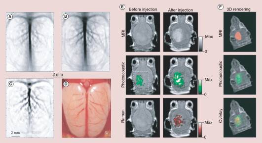
Figure 1. Non-invasive photo-acoustic imaging of a rat’s cerebral cortex using nano-particles as contrast agents. This figure is from [49].

In the sequel, to describe our approach, we will mainly focus on the acoustic imaging using micro-bubbles, i.e. (1), and the photo-acoustic imaging using (dielectric) nano-particles, i.e. (3). In Figure 1 and Figure 2, we see the sharpness of the images when injecting nano-particles or micro-bubbles respectively in the targeted regions. This suggests, in particular, that contrasting the images taken before and after injecting the small-scaled contrasts agents would allow us to extract quantitative information on the targeted regions, as the mass density and the bulk modulus, for the acoustic imaging, or the electric permittivity, and eventually the conductivity, for the photo-acoustic imaging of the targeted region. Our aim is to understand and quantify this.

At the mathematical analysis level, we need to study how the acoustic pressure and the electromagnetic waves (for the related imaging modalities) are perturbed by the presence of micro-bubbles or nano-particles having highly singular relative densities and/or bulks or relative electric permittivity or relative magnetic permeability. For both the two imaging modalities we described above, we need to handle non periodic distributions of the small scaled inclusions and hence homogenization type techniques do not apply. In addition, of a particular importance to us is the use of micro and nano-scaled inclusions which are nearly resonating. In our settings, by resonance we mean the frequencies of incidence for which the corresponding forward problem has non-unique solutions. They are solutions of nonlinear dispersion equations. Basically, in such situations, any solution is a linear combination of one which has a finite energy (fixed by the radiation condition) and others which are localized near the small inclusions. In general, and surely in our settings, such resonances are located in the (lower half of the) complex plane. But if we use micro or nano-scaled inclusions which have, in addition, high contrasts, then these resonances are, in fact, close, in terms of the scales and contrasts, to the real line. This fact will be extensively used in both the imaging modalities.

The analysis is based on integral equation methods (both direct and indirect representations), taking into account the different scales related to the size, contrasts and the eventual cluster of the particles. We highlight few of the key arguments in analyzing these imaging modalities:

1. Rewriting the related Lippmann-Schwinger integral equation for the acoustics (or system for the electromagnetics) as a linear combination of the surface double layer operator (or the Neumann-Poincaré operator) and the volume integral operator (or the Newtonian operator), we show that the eventual resonances split into two families: one given by surface-like eigenfunctions and the other body-like eigenfunction corresponding to the eigenvalues of the Neumann-Poincaré and the Newtonian operators respectively. For instance, we have the Minnaert resonance which corresponds to the value $-\frac{1}{2}$ as the eigenvalue of the Neumann-Poincaré operator, for acoustics, and the plasmonic resonances related to the eventual sequence of eigenvalues to the same operator for the electromagnetism. On the other hand, the dielectric (or Mie) resonances correspond to the eigenvalues of the Newtonian operator for electromagnetism. These resonances can be, approximately, excited if the material properties of the particles enjoy precise scales of their contrasts with the surrounding background. Such scales will be discussed in section 2.

2. The Neumann-Poincaré operator, or the double layer operator, appears due to the contrast of the higher order coefficient as the density for the acoustics model or the permeability for the electromactism model when written solely with the electric fields. It is then not surprising that the dominant terms of the surface-like resonances, i.e. Minnaert for acoustics and plasmonics for electromagntics, depend on that contrast. This is indeed the case as it will shown in section 4. This feature will be of importance in acoustic imaging to reconstruct the mass density. Contrary to these resonances, the volume-like ones (as the dielectric resonances) have their dominant parts independent on the corresponding contrasts (i.e. the contrast of the permittivity and eventually the conductivity).

3. The distribution of the small particles is not necessarily periodic, as we handle single particles, doubles (dimers, i.e. closely spaced two by two particles) and also clusters of highly dense particles. Therefore, homogenization techniques are not useful at this point. Rather, the method of analysis we use has its roots back to the Foldy formal method, see [32, 51], of representing the acoustic field, due to multiple point-like potentials. The multiplicative coefficients attached to these point-like potentials model the scattering strengths (that we call the scattering coefficients). The close form of the Foldy field, solution describes the field generated after all the mutual interaction between the point-like scatterers. Such a representation of the fields has been justified by Berezin and Faddeev in the frame work of quantum mechanics, see [20]. The idea is that based on the Krein extension theory of self-adjoint operators, one can model the diffusion by point-like particles by the Schröedinger model with singular potentials of Dirac type supported on those point-like scatterers. This opened different and fertile directions of research related to modeling with singular potentials supported on point, see [2], lines [29] or generally hypersurfaces [50]. Going back to our subject, and as our small-scaled particles enjoy high contrasts, it is natural then to expect that the dominant part of the field generated by their mutual interactions is reminiscent to the Foldy field. Indeed, this dominating field can be seen as a Foldy field generated by the point-like potentials, centered at the centers of our small particles, where the attaching coefficients, i.e. the scattering coefficients in Foldy’s language, are described by a combination of the used incident frequencies and the relative contrasts of the material (mass density for acoustics or permeability for electromagnetism for instance). This combination is nothing but the dominant part appearing in the (nonlinear) dispersion equation. These scattering coefficients can be large when the incident frequency is taken close to the different resonances mentioned above (depending of the scales of our model). This enhancement of the scattered field is the key step in all the imaging modalities we have cited above. To give a taste on how this is used, let us mention the following three situations:

   
   

   1. Injecting one single particle, the Foldy field reduce to one element, as there is no multiple scattering. In acoustic imaging, we can see from the remotely measured acoustic field, i.e. the far-field for instance, that its value changes drastically whether or not the used incident frequency is close to the resonance (the Minnaert resonance in this case). This discrimination allows us to estimate this resonance. From this resonance, we can estimate the mass density of the background in the vicinity of the injected bubble, see [26]. In photo-acoustics, we could estimate the internal modulus of the total field (i.e. phaseless total field). This allows us to transform the photo-acoustic imaging to the inversion of the phaseless total electric field, see [33].

   2. Injecting dimers, i.e. two close particles, then the Foldy field encodes the multiple scattering field between the two particles. From these fields, we can extract not only the total fields on the two centers, but also the background Green’s function on the two centers. This Green’s function evaluated on the two centers encodes the values of the lower coefficients of our models, i.e. the bulk modulus for acoustic imaging and the permittivity (and eventually the conductivity) for the photo-acoustic imaging, see [33]. However, extracting such information is possible only if the used incident frequencies are close to the mentioned resonances. This issue is related to the Foldy-Lax paradigm, an outstanding open question, on the possibility of extracting, from remote data (i.e. far-fields), the fields generated after multiple scattering between the particles. This paradigm makes sense and it is justified if the used incident frequencies are close to the resonances, see [34].

   3. Injecting a dense cluster of small particles, the corresponding Foldy field approximates the Lippmann-Schwinger field (i.e. the field solution of the Lippmann-Schwinger equation) with a (contrasting) coefficient given by the average of the mutual scattering coefficients of each particle. The sign of this contrast is fixed by the used incident frequency if it is chosen near to the mentioned resonances. As in the metamaterial theory, up to an appropriate choice of the incident frequency, we generate negative lower order coefficients of the effective medium (bulk modulus for acoustics and permittivity for electromagnetism for instance). Hence the derived effective medium enjoys local coercivity. This local coercivity makes the inverse scattering problem more stable. In particular, the related least-square functional might be convex. Again, recovering such nice properties is possible only if the incident frequencies are close to the mentioned resonances.

Figure 2. (a) Multilocular pancreatic cystic mass revealing intracystic septal enhancement $45$ s after micro-bubble injection with ultrasound. (b) The pattern is confirmed at contrast-enhanced CT. This figure is from [56].

The rest of the manuscript is divide as follows. In section 2, respectively section 3, we give a more precise description of the kind of micro-scaled, respectively nano-scaled, inclusions we will be using and describe qualitatively and quantitatively the generated resonances at the precise needed scales. The formal characterization of the resonances described in this section is well justified in deriving the needed asymptotic expansions of the different related fields. This is stated in section 4 for the acoustic imaging and in section 5 for the photo-acoustic imaging modalities respectively. From these expansions, we describe imaging functional that can be used to effectively extract the needed coefficients from those expansions.

2. Characterization of the contrast agents

2.1. Electromagnetic Nano-particles

Different types of nano-particles are proposed in the literature. Let us cite few of them:

1. To create contrast in the permittivity, carbon nano-tubes, ferroelectric nano-particles and the calcium copper titanate are used, see [18]. Such particles have diameter which is estimated around $10$ nm, or $10^{-8}$ m, and have the relative electrical permittivity of the order $10$ for the carbon nanotubes, $10^{3}$ for ferroelectric nano-particles and around $10^{6}$ for the Calcium copper titanate, see [61]. If the benign tumor is located at the cell level (which means that our imaging target $\Omega$ is that cell), with diameter of order $10^{-5}$m, then the $\Omega$-relative radius of the particles is of the order $a\sim 10^{-3}$. Hence, the relative permittivity of the types of nano-particles are estimated of the order $a^{-r}$ where $r$ is $\frac{1}{3}$ for the carbon nanotubes, $1$ for ferroelectric nano-particles and $2$ for the calcium copper titanate.

2. The human tissue is known to be nonmagnetic. To create magnetic contrasts, it was also proposed in [18] to use iron oxid magnetic nano-particles for imaging early tumors. Such material has a relative permeability of the order between $10^{4}$ and $10^{6}$, see [38], and hence of the order $a^{-r}$ with $r$ between $\frac{4}{3}$ and $2$.

3. Other types of material are given through more involved electric or magnetic susceptibilities. Examples of such nano-particles are those for which the permittivity (similarly the permeability) follow spatial dispersion relation as the ones given by the Drude model, i.e. $\epsilon:=\epsilon_{0}-\frac{\omega_{p}^{2}}{\omega(\omega+i\gamma)}$ $\left(\text{or}\;\mu:=\mu_{0}-\frac{\omega_{p}^{2}}{\omega(\omega+i\gamma)}\right)$ with $\omega_{p}$ as the plasma frequency, $\gamma$ the damping parameter and $\omega$ is our incident frequency.

This shows that for the detection of the tumors using such nano-particles, we can model the ratio of the relative electric permittivity and relative magnetic permeability in terms of the relative size of nano-particles. Inspired on this, we set the following definition:

Definition 2.1.

We call $(D_{m},\epsilon_{m},\mu_{m})$ an electromagnetic nano-particle of shape $D_{m}$ with diameter $a$, of order of few tens of nanometers, and permittivity and permeability $\epsilon_{m},\mu_{m}$ respectively. We call them

1. Electric (or Dielectric) Nano-particles if in addition: $\frac{\epsilon_{m}}{\epsilon_{0}}\sim a^{-r},r>0$ and $\frac{\mu_{m}}{\mu_{0}}\sim 1$ as $a\ll 1$.
   This implies that the relative index of refraction is large, i.e. $\frac{\kappa^{2}_{m}}{\kappa^{2}_{0}}:=\frac{\epsilon_{m}\mu_{m}}{\epsilon_{0}\mu_{0}}\gg 1\mbox{ as }a\ll 1$. Hence the relative speed of propagation $\frac{c_{m}}{c_{0}}:=\frac{\kappa_{0}}{\kappa_{m}}$ is small. But, the contrast of the transmission coefficient is moderate.

2. Magnetic (or Plasmonic) Nano-particles if in addition $\frac{\epsilon_{m}}{\epsilon_{0}}\sim 1$ and $\frac{1}{2}\frac{\mu_{m}+\mu_{0}}{\mu_{m}-\mu_{0}}$ is “very close” to one of the eigenvalues of the Neumann-Poincaré operator (i.e. the adjoint of the double layer operator). This means that the relative speed of propagation is moderate. But the contrast of the transmission coefficient is large. Example of such materials are given by the Drude model described above. Indeed, if $\mu_{m}:=\mu_{0}-\frac{\omega^{2}_{p}}{\omega(\omega+i\gamma)}$, then $\frac{1}{2}\frac{\mu_{m}+\mu_{0}}{\mu_{m}-\mu_{0}}=\frac{1}{2}-\frac{\mu_{0}\,\omega(\omega+i\gamma)}{\omega^{2}_{p}}$. For smooth shapes $D_{m}$, the corresponding double layer operator has its spectrum as $\{\sigma_{n}\}_{n\in\mathbb{N}}\subset[-\frac{1}{2},\frac{1}{2})$ with $0$ as the only accumulation point for the sequences $(\sigma_{n})_{n\in\mathbb{N}}$. Hence the incident frequency $\omega$ and the damping parameter $\gamma$ can be chosen so that $\frac{1}{2}\frac{\mu_{m}+\mu_{0}}{\mu_{m}-\mu_{0}}$ approaches elements of the sequence $(\sigma_{n})_{n\in\mathbb{N}}$.

2.2. Micro-Bubbles

Similar as for the electromagnetic nano-particles, we set the following definition of the micro-bubbles

Definition 2.2.

We call $(D_{m},\rho_{m},k_{m})$ a micro-bubble of shape $D_{m}$ with diameter $a$, of about few tens of micrometers, and mass density and bulk modulus $\rho_{m},k_{m}$ respectively. They are called

1. Low Dense / Low Bulk Bubbles if in addition: $\frac{\rho_{m}}{\rho_{0}}\sim a^{r}$ and $\frac{k_{m}}{k_{0}}\sim a^{r}$ with $r>0$ and then $\frac{c^{2}_{m}}{c^{2}_{0}}:=\frac{\rho_{m}}{k_{m}}\,\frac{\rho_{0}}{k_{0}}\sim 1\mbox{ as }a\ll 1$. This means that the relative speed of propagation $\frac{c^{2}_{m}}{c^{2}_{0}}$ is moderate. But the contrast of the transmission coefficient is large.

2. Moderate Dense / Low Bulk Bubbles if in addition: $\frac{\rho_{m}}{\rho_{0}}\sim 1$ and $\frac{k_{m}}{k_{0}}\sim a^{-r},r>0$, as $a\ll 1$. Such bubbles are not known to exist in nature but they might be designed, see [62]. These properties mean that the relative speed of propagation is small. But the contrast of the transmission coefficient is moderate.

3. Characterization of the key resonances

From the above modeling of the nano-particles as well the micro-bubbles, we observe that they enjoy one of the following properties:

1. the speed of propagation is small and the contrast of the transmission coefficient is moderate. In this case, even though the particle is small, the wave might spend some time inside it, i.e. we might have local body mode (or vibration) if the speed is small under some critical scales. However, there is no surface mode as the transmission coefficient is moderate.

2. the speed of propagation is moderate (not small) and the transmission coefficient is large (or singular as the Drude model). In this case, it is the other way around. We might have surface modes under critical scales of the transmission coefficients but it is unlikely to have body modes as the speed is not small enough.

These differences give rise to different types of resonances for our two types of materials (micro-bubbles and nano-particles). We classify them as follows

1. In the case of Micro-bubbles, we have

   1. the Minnaert resonance which corresponds to a surface-mode for the Low Density / Low Bulk bubbles.

   2. A sequence of resonances which correspond to body-modes for the Moderate Density / Low Bulk bubbles.

2. In the case of nano-particles,

   1. the plasmonic sequence of resonances which corresponds to surface-modes for plasmonic nano-particles.

   2. the Mie (or dielectric) sequence of resonances corresponding to body-modes for the dielectric nano-particles.

Such resonances manifest themselves for special values of $r$. Indeed for $r<2$, they are very large and for $r>2$ they are very small in terms of the relative diameter $a$, $a\ll 1$. However, for $r=2$, they are moderate and their dominant parts are independent of $a$. In the next section, we consider the case $r=2$ and show formally how these resonances indeed appear. For simplicity of the exposition, we handle the cases where the background is homogeneous, i.e. the material coefficients are all constant outside the injected particles. However, the same results occur even for heterogeneous backgrounds.

3.1. Formal characterization of the resonances. The acoustic model

Let $D=z+a\;B$ be a bounded, $C^{1}$-smooth and connected subset containing the origin of $\mathbb{R}^{3}$, with a ’radius’ $a\ll 1$. Let $u=u^{s}+u^{i}$ be the solution of the acoustic scattering problem, see [21, 22, 5, 8],

$$\begin{cases}\mathrm{div}\,\frac{1}{\rho}\nabla u+\omega^{2}\frac{1}{k}u=0\quad\text{in}\;\mathbb{R}^{3},\\ u^{s}:=u-u^{i}\text{ satisfies the following Sommerfeld Radiation Conditions (S.R.C.)}\\ \frac{\partial u^{s}}{\partial|x|}-i\;\omega\sqrt{\frac{\rho}{k}}\;u^{s}=o\left(\frac{1}{|x|}\right),|x|\rightarrow\infty.\end{cases}$$

where

$$\rho:=\begin{cases}\rho_{1}\quad\text{inside }D,\\ \rho_{0}\quad\text{outside }D\end{cases}\text{and}\qquad k:=\begin{cases}k_{1}\quad\text{inside }D,\\ k_{0}\quad\text{outside }D.\end{cases}$$

Here $u^{i}:=u^{i}(x,\omega,\theta):=e^{i\omega\sqrt{\frac{\rho_{0}}{k_{0}}}\;x\cdot\theta}$ is an incident plane wave propagating in the direction $\theta$.

From the Lippmann-Schwinger representation of the total acoustic field $u$, we have

(3.1) $$u(x)-\alpha\,\underset{x}{\mathrm{div}\,}\int_{D}G_{\omega}(x-y)\nabla u(y)dy-\beta\omega^{2}\int_{D}G_{\omega}(x-y)u(y)dy=u^{i}(x),$$

where $\alpha:=\frac{1}{\rho_{1}}-\frac{1}{\rho_{0}}$ and $\beta:=\frac{1}{k_{1}}-\frac{1}{k_{0}}$ represent the contrasts between the inner and the outer acoustic coefficients. Here, $G_{\omega}$ is the Green’s function of the background medium $(\rho_{0},k_{0})$ satisfying the outgoing Sommerfeld radiation conditions. This is an integro-differential equation. To transform it to a solely integral equation, we proceed by integration by parts then (3.1) becomes

$$u(x)-\gamma\omega^{2}\int_{D}G_{\omega}(x-y)u(y)dy+\alpha\int_{\partial D}G_{\omega}(x-y)\frac{\partial u}{\partial\nu}(y)dy=u^{i}(x),$$

where $\gamma:=\beta-\alpha\rho_{1}/k_{1}$, for $x\in D$. In addition, taking the normal derivative and trace, with the usual traces of the double layer potential, we obtain:

$$(1+\frac{\alpha}{2})\frac{\partial u}{\partial\nu}-\gamma\omega^{2}\partial_{\nu-}\int_{D}G_{\omega}(x-y)u(y)dy+\alpha(K_{D}^{\omega})^{*}[\frac{\partial u}{\partial\nu}]=\frac{\partial u^{i}}{\partial\nu}.$$

Hence for $x\in\mathbb{R}^{3}\setminus\overline{D}$, the total acoustic field $u(x)$ is characterized by $u|_{D}$ and $\frac{\partial u}{\partial\nu}|_{\partial D}$ which are solutions of the following close form system of integral equations:

$$[I-\gamma\omega^{2}N^{\omega}]u+\alpha\int_{\partial D}G_{\omega}(x-y)\frac{\partial u}{\partial\nu}(y)dy=u^{i}(x),\;\mbox{ in }D$$

$$[\frac{1}{\alpha}+\frac{1}{2}+(K_{D}^{\omega})^{*}][\frac{\partial u}{\partial\nu}]-\frac{\gamma}{\alpha}\omega^{2}\partial_{\nu-}\int_{D}G_{\omega}(x-y)u(y)dy=\frac{1}{\alpha}\frac{\partial u^{i}}{\partial\nu},\;\mbox{ on }\partial D$$

with the Newtonian (a volume-type) operator:

$$N^{\omega}:L^{2}(D)\longrightarrow L^{2}(D),\leavevmode\nobreak\ \leavevmode\nobreak\ \leavevmode\nobreak\ N^{\omega}(u)(x):=\int_{D}G_{\omega}(x-y)u(y)dy,$$

with image of $N^{\omega}$ in $H^{2}(D)$, and the Neumann-Poincaré (a surface-type) operator

$$(K_{D}^{\omega})^{*}:H^{-1/2}(\partial D)\longrightarrow H^{-1/2}(\partial D),\leavevmode\nobreak\ \leavevmode\nobreak\ \leavevmode\nobreak\ (K_{D}^{\omega})^{*}(f)(x):=p.v.\int_{\partial D}\frac{\partial}{\partial\nu_{x}}G_{\omega}(x-y)f(y)dy.$$

Remark 3.1.

The following properties are key in estimating the resonances. For $\omega=0$, each of these operators generates a sequence of eigenvalues: $\lambda_{m}(N^{0})\stackrel{{\scriptstyle m\rightarrow\infty}}{{\longrightarrow}}0$ and $\sigma_{p}((K_{D}^{0})^{*})\subset[-\frac{1}{2},\frac{1}{2})$. In addition, we have $K^{0}_{D}(1)=-\frac{1}{2}$. These singular values are behind all the used resonances.

Indeed, let us recall the system of integral equation and see how it behaves for the scales defining our micro-bubbles:

(3.2) $$\left[I-\gamma\leavevmode\nobreak\ \omega^{2}\leavevmode\nobreak\ N^{\omega}\right]u+\alpha\int_{\partial D}G_{\omega}(x-y)\frac{\partial u}{\partial\nu}(y)dy=u^{i}(x),\;\mbox{ in }D,$$

(3.3) $$\left[\frac{1}{\alpha}+\frac{1}{2}+(K_{D}^{\omega})^{*}\right]\left[\frac{\partial u}{\partial\nu}\right]-\frac{\gamma}{\alpha}\omega^{2}\partial_{\nu-}\int_{D}G_{\omega}(x-y)u(y)dy=\frac{1}{\alpha}\frac{\partial u^{i}}{\partial\nu},\;\mbox{ on }\partial D.$$

1. For Low Density / Low Bulk bubbles, we have $\gamma\sim 1$ and then $\gamma\,\omega^{2}\,N^{\omega}\ll 1$ as $a\ll 1$. Hence, there is no singularity coming from (3.2). But as $\alpha\gg 1$, precisely if $\alpha\sim a^{-2}$ as $a\ll 1$, then we can excite the eigenvalue $-\frac{1}{2}$ of $K_{D}^{0}$ and create a singularity in (3.3). In this case, we have the Minnaert resonance with surface-modes. This resonance was first observed in [8] based on indirect integral equation methods. This observation was used for different purposes, see [9, 10, 11, 12]. This result was extended to more general families of micro-bubbles in [5, 6].

2. For Moderate Density / Low Bulk bubbles, we have $\alpha\sim 1$ and then we keep away from the full spectrum of $(K_{D}^{0})^{*}$. Hence there is no singularity coming from (3.3). But as $\gamma\sim a^{-2}\gg 1$, we can excite the eigenvalues of the Newtonian operators $N^{0}$ and create singularities in (3.2). This gives us a sequence of resonances with volumetric-modes. This was observed in [7] and [52].

3. Observe that if $\alpha$ is negative (i.e. negative mass densities, similar to the Drude model for acoustics for instance) then we could excite the other sequence of eigenvalues of $(K_{D}^{0})^{*}$. This gives us another sequence of resonances (i.e. corresponding to the sequence of plasmonics in electromagnetics, see section 3.2).

Using Lippmann-Schwinger equations allows to characterize all these resonances and for varying backgrounds (i.e. heterogeneous backgrounds), see [26].

3.2. Formal characterization of the resonances. The electromagnetic model

We deal with non-magnetic materials. The electric field $E=E^{s}+E^{i}$ is solution of the electromagnetic scattering problem, see [24, 27],

$$\begin{cases}curl\;curl\;E+\omega^{2}\,\epsilon\,\mu_{0}\,E=0\quad\text{in }\mathbb{R}^{3},\\ E^{s}:=E-E^{i}\text{ satisfies the following Silver-Mueller Radiation Condition (S-M.R.C.)}\\ \underset{|x|\rightarrow\infty}{\lim}\left(curl\;E^{s}(x)\times x-i\;\omega\sqrt{\epsilon\;\mu_{0}}\;|x|\;E^{s}(x)\right)=0\end{cases}$$

where

$$\epsilon:=\begin{cases}\epsilon_{1}\quad\text{inside }D,\\ \epsilon_{0}\quad\text{outside }D.\end{cases}$$

Here, $E^{i}$ is a polarized incident electric field propagating in the background medium. In particular, it is divergence free, i.e. $\nabla\cdot E^{i}=0$ in the whole space.

The corresponding Lippmann-Schwinger equation is:

(3.4) $$E(x)+\eta\;\underset{x}{\nabla}\;\int_{D}\underset{y}{\nabla}G_{\omega}(x-y)\cdot E(y)dy-\omega^{2}\eta\int_{D}G_{\omega}(x-y)E(y)dy=E^{i}(x),$$

where $\eta:=\epsilon_{1}-\epsilon_{0}$ is the contrast of the inner and outer electric permittivities. Here, $G_{\omega}$ is the Green’s function of the Helmholtz equation $(\Delta+\omega^{2}\epsilon_{0}\;\mu_{0})=-\delta,$ satisfying the Sommerfeld outgoing radiation condition. By integration by parts, (3.4) becomes

$$E(x)-\eta\omega^{2}\int_{D}G_{\omega}(x-y)E(y)dy+\eta\nabla\int_{\partial D}G_{\omega}(x-y)E\cdot\nu(y)dy=E^{i}(x).$$

In addition, taking the normal limit from inside $D$, we obtain:

$$(1+\frac{\eta}{2})E\cdot\nu-\eta\,\omega^{2}\,\nu\cdot\int_{D}G_{\omega}(x-y)E(y)dy+\eta(K_{D}^{\omega})^{*}[E\cdot\nu]=E^{i}\cdot\nu,\;\mbox{ on }\partial D.$$

Hence for $x\in\mathbb{R}^{3}\setminus\overline{D}$, $E(x)$ is characterized by $E|_{D}$ and $E\cdot\nu|_{\partial D}$ which are solutions of the close system of integral equation:

(3.5) $$\left[I-\eta\omega^{2}N^{\omega}\right]E+\eta\,\nabla\int_{\partial D}G_{\omega}(x-y)E\cdot\nu(y)dy=E^{i}(x),\;\mbox{ in }D$$

and

(3.6) $$\left[\frac{1}{\eta}+\frac{1}{2}+(K_{D}^{\omega})^{*}\right][E\cdot\nu]-\omega^{2}\nu\cdot\int_{D}G_{\omega}(x-y)E(y)dy=\frac{1}{\eta}\;E^{i}\cdot\nu,\;\mbox{ on }\partial D.$$

1. For dielectric nano-particles, we have $\eta\gg 1$. Hence $\frac{1}{\eta}\ll 1$, however we keep away from the full spectrum of $(K_{D}^{0})^{*}$ as the dominating term of the sources is $\frac{1}{\eta}\;E^{i}\cdot\nu$ which is average-zero as $\nabla\cdot E^{i}=0$. Hence no singularity comes form (3.6). But if in addition $\eta\sim a^{-2}\gg 1$, then we can excite the eigenvalues of the Newtonian operators $N^{0}$ and create singularities in (3.5). Observe here that the Newtonian operator is vectorial in contrast to the acoustic case where it is a scalar operator. Therefore its spectral decomposition is more involved. Nevertheless, projecting it on the subspace of divergence free fields in $D$ with zero normal component on $\partial D$, we obtain the sequence of dielectric (or Mie) resonances.

2. Observe that if the real part of $\eta$ is negative (i.e. negative contrast permittivity) as in the Drude model, where $\eta=\epsilon-\epsilon_{0}=-\frac{\omega_{p}^{2}}{\omega(\omega+i\;\gamma)}$, then we can excite the sequence of eigenvalues of $(K_{D}^{0})^{*}$, which lie in $[-\frac{1}{2},\;\frac{1}{2})$, by appropriately choosing the damping parameter $\gamma$ and the incident frequency $\omega$. This gives us the sequence of electric plasmonics which create singularities in (3.6). With such material contrast $\eta$, there is no singularity that can be created in (3.5), since $N^{\omega}$ scales as $a^{2},\;a\ll 1$.

3. It is legitimate to ask if any resonance, corresponding to the Minnaert one in Acoustics, exists? To answer to this question, we consider magnetic materials, i.e. $\mu_{1}\neq\mu_{0}$. In the TM-approximation, the magnetic component $u:=H_{3}$, satisfies the acoustic scattering problem

$$\begin{cases}\mathrm{div}\,\frac{1}{\epsilon}\nabla u+\omega^{2}\mu u=0\quad\text{in }\mathbb{R}^{2},\\ u^{s}\text{ satisfies the S.R.C}\end{cases}$$

where $\epsilon=\epsilon_{1}$ inside $D$, $\epsilon=\epsilon_{0}=1$ outside $D$, $\mu=\mu_{1}$ inside $D$, $\mu=\mu_{0}=1$ outside $D$. As in the Acoustic case, for $x\in\mathbb{R}^{3}\setminus\overline{D}$, $u(x)$ is characterized by   $u|_{D}$   and   $\frac{\partial u}{\partial\nu}|_{\partial D}$   which satisfy the system:

$$\begin{cases}\left[I-\tilde{\gamma}\,\omega^{2}\,N^{\omega}\right]u+\tilde{\alpha}\int_{\partial D}G_{\omega}(x-y)\frac{\partial u}{\partial\nu}(y)dy=u^{i}(x),\;\mbox{ in }D\\ \,\\ \left[\frac{1}{\tilde{\alpha}}+\frac{1}{2}+(K_{D}^{\omega})^{*}\right][\frac{\partial u}{\partial\nu}]-\frac{\gamma}{\tilde{\alpha}}\omega^{2}\partial_{\nu-}\int_{D}G_{\omega}(x-y)u(y)dy=\frac{1}{\tilde{\alpha}}\frac{\partial u^{i}}{\partial\nu},\;\mbox{ on }\partial D\end{cases}$$

where, now, $\tilde{\gamma}:=\frac{\epsilon_{1}\mu_{1}}{\epsilon_{0}}-\mu_{0}\mbox{\leavevmode\nobreak\ \leavevmode\nobreak\ and\leavevmode\nobreak\ \leavevmode\nobreak\ }\tilde{\alpha}:=\epsilon^{-1}_{1}-\epsilon^{-1}_{0}.$

1. Hence $\tilde{\gamma}\sim 1$ if the index of refraction is moderate, i.e. $\epsilon_{1}\mu_{1}\sim 1$. Then $\gamma\,\omega^{2}\,N^{\omega}\ll 1$ as $a\ll 1$.

2. In addition $\tilde{\alpha}\gg 1$ if $\epsilon_{1}\ll 1$, as $a\ll 1$. Then we can excite the eigenvalue $-\frac{1}{2}$ of $K_{D}^{0}$.

Hence, a Minnaert-like resonance can be excited by $\epsilon$-near-zero and $\mu$-near-infinity nano-particles. The last issue is whether such materials exist in nature or possible to be designed. Material with $\epsilon$-near-zero are possible with the Drude model where $\epsilon:=\epsilon_{0}-\frac{\omega^{2}_{p}}{\omega(\omega+i\;\gamma)}$ choosing $\gamma,\gamma\ll 1$, and $\omega$ so that $\epsilon$ is near zero.

3.3. Summary on the existence of the resonances

We summarize here the possibilities we have in creating resonances.

1. Acoustic bubbles:

   • For low density / low bulk bubbles, we have the Minnaert resonance with surface-modes.

   • For moderate density / low bulk bubbles, we have a sequence of resonances with volumetric-modes.

   • For negative contrasts of mass densities, we have a sequence of resonances (corresponding to the plasmonics in electromagnetism) with surface-modes.

2. Electromagnetic nano-particles:

   • For dielectric nano-particles, we have the sequence of Mie (or dielectric) resonances with volumetric-modes.

   • For negative contrast of the permittivity, as Drude’s model, we have the sequence of plasmonic resonances with surface-modes.

   • For $\epsilon$-near-zero and $\mu$-near-infinity nano-particles, we have one more resonance (corresponding to the Minnaert one in acoustic bubbles) with surface-modes.

4. Acoustic imaging using resonating micro-bubbles

4.1. Expansion of the fields

Let $D:=z+a\;B$ be the bubble of center $z$ injected in the body to image $\Omega$ which is a bounded and smooth domain in $\mathbb{R}^{3}$.

Let $v:=v^{s}+v^{i}$ be the total field generated by the background $(\rho_{0},k_{0})$ without the bubble. Here the coefficients $(\rho_{0},k_{0})$ are variable and $W^{1}$-smooth inside $\Omega$ and $(\rho_{0},k_{0}):=(\rho_{0,\infty},k_{0,\infty})$ outside $\Omega$ where $\rho_{0,\infty}$ and $k_{0,\infty}$ are positive constants.

We set $u:=u^{s}+u^{i}$ to be the total field generated by the background $(\rho,k)$ in the presence of one bubble. This means that $(\rho,k)=(\rho_{1},k_{1})$ inside the bubble $D$ and $(\rho,k)=(\rho_{0},k_{0})$ outside of it. Here $v^{i}=u^{i}:=e^{i\kappa_{0}\theta\cdot x}$ is the incident plane wave where $\kappa_{0}:=\omega\sqrt{\frac{\rho_{0,\infty}}{k_{0,\infty}}}$ and $\theta$ is the direction of incidence. Hence, the acoustic model in the presence of one bubble injected in the heterogeneous background $\Omega$ reads as follows, see [21, 22, 5, 8],

$$\begin{cases}\mathrm{div}\,\frac{1}{\rho}\nabla u+\omega^{2}\frac{1}{k}u=0\quad\text{in }\mathbb{R}^{3},\\ u^{s}:=u-u^{i}\text{ satisfies (S.R.C.).}\end{cases}$$

Due to the Sommerfeld radiation condition, we have the following behavior of the scattered field $u^{s}(x,\theta)$ far away from the target region $\Omega$:

$$u^{s}(x,\theta)=\frac{e^{i\kappa_{0}|x|}}{|x|}u^{\infty}(\hat{x},\theta)+\mathcal{O}\left(|x|^{-2}\right),\;\;|x|\to+\infty,$$

where $\hat{x}:=x/|x|$ and $u^{\infty}(\hat{x},\theta)$ denotes the far-field pattern corresponding to the unit vectors $\hat{x},\theta$, i.e. the incident and propagation directions respectively.

Here we take the scales $k_{1}:=\bar{k}_{1}\;a^{2}\leavevmode\nobreak\ \mbox{ and }\leavevmode\nobreak\ \rho_{1}:=\bar{\rho}_{1}\;a^{2},$ where $\bar{k}_{1}$ and $\bar{\rho}_{1}$ are positive constants independent of $a$. With these scales, we have existence of the Minnaert resonance. Indeed, we have the expansion, see [26]:

(4.1) $$u^{\infty}(\hat{x},\theta,\omega,z)=v^{\infty}(\hat{x},\theta,\omega)-\frac{1}{\overline{k}_{1}}\;\frac{\omega^{2}_{M}}{\omega^{2}-\omega^{2}_{M}}|B|\;a\;v(z,-\hat{x},\omega)\;v(z,\theta,\omega)+O\left(\frac{a^{2}}{\left(\omega^{2}-\omega^{2}_{M}\right)^{2}}\right)$$

where

(4.2) $$\omega_{M}=\omega_{M}(z):=\sqrt{\frac{8\,\pi\,\overline{k}_{1}}{\rho_{0}(z)\,A_{\partial B}}}\leavevmode\nobreak\ \leavevmode\nobreak\ \leavevmode\nobreak\ (\emph{\leavevmode\nobreak\ The\leavevmode\nobreak\ Minnaert\leavevmode\nobreak\ resonance!})$$

with $A_{\partial B}:=\frac{1}{\left|\partial B\right|}\int_{\partial B}\int_{\partial B}\frac{(x-y)\cdot\nu(x)}{4\pi|x-y|}dxdy.$

The far-field $u^{\infty}(\hat{x},\theta,\omega,z)$ depends on the frequency of incidence $\omega$ and also the injected bubble at the point $z$, that is why we added the parameter $z$. The far-field $v^{\infty}(\hat{x},\theta,\omega)$ corresponds to scattering by the background but without the bubble, hence the parameter $z$ is not added.

4.2. Solution of the inverse problem using one injected bubble

The acoustic imaging problem we are interested in is to reconstruct the background coefficients $k_{0}$ and $\rho_{0}$ inside the imaging target $\Omega$. For this, we need the following data.

1. The back-scattered far-field $v^{\infty}(-\theta,\theta,\omega)$ in one single direction $\theta$ measured before injecting any bubble.

2. The back-scattered far-field $u^{\infty}(-\theta,\theta,\omega,z)$ in one single direction $\theta$ measured for each injected bubble, located in a point $z\in\Omega$.

We use these data for a band of frequencies

$$[\omega^{min}_{M},\leavevmode\nobreak\ \leavevmode\nobreak\ \omega^{max}_{M}]$$

where

$$\omega^{min}_{M}<\sqrt{\frac{4\,\pi\,\overline{k}_{1}}{\Big{(}\underset{\Omega}{\max}\,\rho_{0}(z)\Big{)}\leavevmode\nobreak\ \;A_{\partial B}}}\;\mbox{ and }\;\omega^{max}_{M}>\sqrt{\frac{4\,\pi\,\overline{k}_{1}}{\Big{(}\underset{\Omega}{\min}\,\rho_{0}(z)\Big{)}\;\leavevmode\nobreak\ A_{\partial B}}}.$$

The imaging procedure goes as follows. We set

(4.3) $$I(\omega,z):=u^{\infty}(-\theta,\theta,\omega,z)-v^{\infty}(-\theta,\theta,\omega)$$

as the imaging functional, remembering that the incident angle $\theta$ is fixed. We have the following properties from (4.1)

(4.4) $$I(\omega,z)\sim-\frac{\omega^{2}_{M}}{\overline{k}_{1}(\omega^{2}-\omega^{2}_{M}(z))}|B|\;a\;\;[v(z,\theta,\omega)]^{2}.$$

We divide this procedure into two steps:

1. Step 1. From this expansion, we recover $\omega^{2}_{M}(z)$ as the frequency for which the imaging function $\omega\rightarrow I(\omega,z)$ gets its largest value. From the estimation of this resonance $\omega^{2}_{M}(z)$, we reconstruct the mass density at the center of the injected bubble $z$, based on (4.1), as follows:

   $$\rho_{0}(z)=\frac{4\pi\,\overline{k}_{1}}{\omega^{2}_{M}(z)\;A_{\partial B}}.$$

   Scanning the domain $\Omega$ by such bubbles, we can estimate the mass density there.

2. Step 2. To estimate now the bulk modulus, we go back to (4.4) and derive the values of the total field $[v(z,\theta,\omega)]^{2}$. This field corresponds to the model without the bubble. Hence, we have at hand $v(z,\theta,\omega)$ for $z\in\Omega$ up to a sign (i.e. we know the modulus and the phase up to a multiple of $\pi$). Use the equation $\nabla\cdot\rho^{-1}_{0}\nabla v+\omega^{2}k^{-1}_{0}v=0$ to recover the values of $k_{0}$ in the regions where $v$ does not change sign. This can be done by numerical differentiation for instance. Other ways are of course possible to achieve this second step. In addition, we have at hand multiple frequency internal data.

The procedure described above uses the Minnaert resonance. The key point to recover the mass density is the explicit dependance of this resonance on the value of the mass density, of the background, on it’s ’center’, see (4.2).

Remark 4.1.

We have shown that using multifrequency back-scattering data at one single frequency, we can reconstruct the mass density with a simple and explicit formula. In addition, we can estimate the internal values of total field from which we derive the values of the bulk modulus via numerical differentiation. Disadvantages of this procedure are as follows:

• Possible zeros of the total fields $v(z,\theta,\omega_{M}(z))$. Indeed, we cannot recover the bulk modulus $k_{0}$ in the regions where this total field vanishes. But this is natural and cannot be avoided without extra information. One way to handle this issue is to use multiple directions of incidence $\theta$.

• Numerical differentiation. The numerical differentiation is an unstable step. In addition, we need to differentiate twice reconstructed, and hence noisy, quantities given by $\rho_{0}$ and $v$. This makes it a difficult issue to handle in practice. One way to remedy to this is to use two injected bubbles which are close to each other. Doing so, we can recover not only the total field $v$ but also the Green’s function $G_{\omega_{M}}$, of the background medium, on the ’centers’ of the two bubbles. From the singularities of $G_{\omega_{M}}$, we recover the bulk $k_{0}$. The idea of the proof is based on the Foldy-Lax paradigm on whether one can extract the multiple scattering field generated by closely spaced small particles from the measured far-field. This paradigm is justified for nearly resonating frequencies. This argument was tested in a similar situation, see [3]. A complete study of this paradigm for our settings is done in [34].

4.3. Summary on the Acoustic imaging using resonating bubbles

Here, we summarize the way how we propose to solve the acoustic imaging problem.

1. Injecting single bubbles and using the generated back-scattered field in one incident direction, sent at multiple frequencies, we can reconstruct

   1. the density $\rho_{0}$ via direct and stable formulas,

   2. the bulk $k_{0}$ with numerical differentiation.

2. Injecting double and close bubbles (i.e. dimers), we can avoid the numerical differentiation.

5. Photo-acoustic imaging using resonating nano-particles

5.1. The mathematical model

The photo-acoustic experiment, in the general setting, applies to targets that are electrically conducting, in other words the imaginary part of the ’permittivity’ is quite pronounce, and it goes as follows. Exciting the target, with laser, or by sending an incident electric field, will create heat in it surrounding. This heat, in its turn, creates fluctuations, i.e. a pressure field, that propagates along the body to image. This pressure can be collected in an accessible part of the boundary of the target. The photo-acoustic imaging is to trace back the pressure and reconstruct the permittivity that created it.

To describe the mathematical model behind this experiment, let us set $E$, $\bm{T}$ and $p$ to be respectively the electric field, the heat temperature and the acoustic pressure. Then, as described above, the photo-acoustic experiment is based on the following model coupling these three quantities:

$$\left\{\begin{array}[]{llrr}curl\;curl\;E-\omega^{2}\;\varepsilon\;\mu_{0}\;E=0,\leavevmode\nobreak\ \leavevmode\nobreak\ \leavevmode\nobreak\ E:=E^{s}+E^{i},\mbox{ in }\mathbb{R}^{3},\\ \\ \rho_{0}c_{p}\dfrac{\partial\bm{T}}{\partial t}-\nabla\cdot\kappa\nabla\bm{T}=\omega\;{\mathrm{Im\,}}(\varepsilon)\;|E|^{2}\;\delta_{0}(t),\;\mbox{ in }\mathbb{R}^{3}\times\mathbb{R}_{+},\\ \\ \dfrac{1}{c^{2}}\dfrac{\partial^{2}p}{\partial t^{2}}-\Delta p=\rho_{0}\;\beta_{0}\;\dfrac{\partial^{2}\bm{T}}{\partial t^{2}},\mbox{ in }\mathbb{R}^{3}\times\mathbb{R}_{+},\end{array}\right.$$

where $\rho_{0}$ is the mass density, $c_{p}$ the heat capacity, $\kappa$ is the heat conductivity, $c$ is the wave speed and $\beta_{0}$ the thermal expansion coefficient. To the last two equations, we supplement the homogeneous initial conditions:

$$\bm{T}=p=\frac{\partial p}{\partial t}=0,\mbox{ at }t=0$$

and the Silver-Mueller radiation condition to $E^{s}$. More details on the actual derivation of this model can be found in [57, 60] and more references therein.

In our settings, the source of the heat is given by the injected electromagnetic nano-particles. Precisely, we propose to inject dielectric nano-particles. As described in section 2 and section 3, these nano-particles enjoy the following features. They are highly localized as they are nano-scaled and they have high contrast permittivity. Under critical scales, that will be described later, these two features allow us to estimate the dominant part of the measure pressure and then extract from it the unknown permittivity, and eventually the conductivity as well.

To give more details on how such procedure works, we restrict ourselves to

1. the 2D-TM model for the electromagnetic propagation.

2. the heat conductivity $\kappa$ is small and can be neglected.

Under such conditions, the $2D$ model of the photo-acoustic reduces to one single equation, see [60].

(5.1) $$\left\{\begin{array}[]{rll}\partial^{2}_{t}p(x,t)-c_{s}^{2}(x)\Delta_{x}p(x,t)&=&0\qquad in\quad\mathbb{R}^{2}\times\mathbb{R}^{+}.\\ p(x,0)&=&\frac{\omega\,\beta_{0}}{c_{p}}{\mathrm{Im\,}}(\varepsilon)(x)\,|E_{3}|^{2}(x),\qquad in\quad\mathbb{R}^{2}\\ \partial_{t}p(x,0)&=&0\qquad in\quad\mathbb{R}^{2}\end{array}\right.$$

here $c_{s}$ is the velocity of sound in the medium that is smooth and $c_{s}-1$ is supported in a smooth and compact set $\Omega$. The constants $\beta_{0}$ and $c_{p}$ are known and $\omega$ is an incident frequency. The source $u:=E_{3}$ is solution of the scattering problem

(5.2) $$\left\{\begin{array}[]{rll}\Delta u+\omega^{2}\mu_{0}\epsilon\;u=0\quad\text{in }\mathbb{R}^{2},\\ \\ u(x):=u^{s}(x)+e^{i\;\omega\sqrt{\mu_{0}\epsilon_{0}}\;x}\\ \\ u^{s}\text{ satisfies the S.R.C.}\end{array}\right.$$

where $\epsilon=\epsilon_{1}$ inside $D$, $\epsilon=\epsilon_{0}$ outside $D$ and $\epsilon_{0}=1$ outside $\Omega$ ($D\subset\Omega$ being the injected nano-particle). The permittivity $\epsilon_{0}$ is variable and it is supposed to be Lipschitz smooth inside $\Omega$.

5.2. Inversion of the photo-acoustics using nano-particles

The goal of the photo-acoustic imaging using nano-particles is to recover $\epsilon$ in $\Omega$ from the measure of the pressure $p(x,t),\;x\in\partial\Omega$ and $t\in(0,T)$ for large enough $T$. The decoupling of the original photo-acoustic mathematical model (5.1) into (5.1)-(5.2) suggests that we split the inversion into the following two steps.

1. Acoustic Inversion: Recover the source term ${\mathrm{Im\,}}(\varepsilon)(x)\,|u|^{2}(x)$, $x\in\Omega$, from the measure of the pressure $p(x,t),\;x\in\partial\Omega$ and $t\in(0,T)$.

2. Electromagnetic Inversion: Recover the permittivity $\epsilon(x),\;x\in\Omega$ from ${\mathrm{Im\,}}(\varepsilon)(x)\,|u|^{2}(x)$, $x\in\Omega$.

The pressure is collected on the boundary of $\Omega$ in the following situations:

• Before injecting any particle.   There is a considerable amount of works in the literature based on such data. Without being exhaustive, we cite the following references [4, 17, 19, 14, 15, 16, 25, 31, 41, 46, 47, 53, 54, 58, 59] devoted to such inversions.

• After injecting a single particle. To our best knowledge, there is only the work [60] where plasmonic nano-particles are used and an optimization method was proposed to invert the electric energy fields. There, the $2D$-model is stated and the magnetic field was used.

• After injecting a double and close particles (dimers).

• After injecting a cluster of particles.

In the sequel, we show how we can use the data given by the second, third, or forth possibilities to solve the photo-acoustic imaging problem using dielectric nano-particles.

5.3. Some Known Acoustic Inversions [46, 47, 54].

Here, we describe two different methods proposed to do the inversion of the acoustic field and recover the initial data. The first one is related to the Radon transform and the second one is based on spectral theory.

1. If the speed of propagation $c_{s}$ is constant and $\Omega$ is a disc of radius $R$, then

   $${\mathrm{Im\,}}(\varepsilon)(x)\,|u|^{2}(x)=\frac{1}{2\pi R}\int_{\partial\Omega}\int_{0}^{2R}(\partial_{r}\,r\,\partial_{r}M({\mathrm{Im\,}}(\varepsilon)\,|u|^{2}))(p,r)\,\log(|r^{2}-|x-p|^{2}|)\,dr\,d\sigma(p)$$

   where

   $$M({\mathrm{Im\,}}(\varepsilon)\,|u|^{2})(x,r)=\frac{2\omega\beta_{0}}{c_{p}\pi}\int_{0}^{c_{s}r}\frac{p(x,t)}{\sqrt{r^{2}-t^{2}}}dt.$$

   See [54] for more details and [31], and the references therein, for further development on the inversion of the Radon transform.

2. Otherwise, but under certain conditions as the non-trapping one, we have the spectral representation

   $${\mathrm{Im\,}}(\varepsilon)(x)\,|u|^{2}(x)=\frac{c_{p}}{\omega\,\beta_{0}}\,\sum_{k}({\mathrm{Im\,}}(\varepsilon)(x)\,|u|^{2})_{k}\psi_{k}(x)$$

   where

   $$({\mathrm{Im\,}}(\varepsilon)(x)\,|u|^{2})_{k}=\lambda^{-2}_{k}g_{k}(0)-\lambda^{-3}_{k}\int_{0}^{\infty}\sin(\lambda_{k}t)\,g^{\prime\prime}_{k}(t)dt$$

   with

   $$g_{k}(t)=\int_{S}p(x,t)\frac{\partial\overline{\psi_{k}}}{\partial\nu}(x)dx$$

   and $(\lambda_{k},\psi_{k})$ is the eigen-system of $-c^{-2}_{s}(x)\Delta$ with zero Dirichlet boundary condition on $\partial\Omega$. See [46, 47] for more details.

5.4. An Approximative Acoustic Inversion [33].

Contrary to the previous described results, here we need no condition on the geometry of the shape of $\Omega$ nor a trapping conditions. We assume the permittivity $\epsilon_{0}(\cdot)$, of the medium, to be $W^{1,\infty}-$smooth in $\Omega$ and the permeability $\mu_{0}$ to be constant and positive. We propose approximative inversions of the acoustic pressure fields to retrieve the initial data under some conditions on localization and large contrast of the permittivity of the injected dielectric nano-particles. Precisely, we assume that the injected nano-particles enjoy the properties:

$${\mathrm{Re\,}}\left(\epsilon_{p}\right)\sim a^{-2}|\log(a)|^{-1}\leavevmode\nobreak\ \leavevmode\nobreak\ \leavevmode\nobreak\ \mbox{and}\leavevmode\nobreak\ \leavevmode\nobreak\ \leavevmode\nobreak\ {\mathrm{Im\,}}\left(\epsilon_{p}\right)\sim a^{-2}|\log(a)|^{-1-h-s},\;\leavevmode\nobreak\ \leavevmode\nobreak\ \leavevmode\nobreak\ s>0.$$

The frequency of the incidence $\omega$ is chosen close to the dielectric resonance $\omega_{n_{0}}$:

$$\omega^{2}_{n_{0}}:=\left(\mu_{0}\,\epsilon_{p}\,\lambda_{n_{0}}\right)^{-1},$$

as follows

(5.3) $$\omega^{2}:=\omega_{\pm}^{2}:={\mathrm{Re\,}}(\omega^{2}_{n_{0}})(1\pm|\log(a)|^{-h}),\;\leavevmode\nobreak\ \leavevmode\nobreak\ 0<h<1$$

where $\lambda_{n_{0}}$ is an eigenvalue of the Newtonian operator acting as:

$$A_{0}u(x):=\int_{D}-\frac{1}{2\pi}\ln(|x-y|)u(y)dy.$$

Let $x\in\partial\Omega$ and $t\geq diam(\Omega)$. Under the condition $0<s<1-h$, we have the following expansions of the pressure:

1. Injecting one nano-particle. In this case, we have the expansion

   $$(p^{+}+p^{-}-2p_{0})(t,x)=\frac{-t\,\omega\,\beta_{0}}{c_{p}\,(t^{2}-|x-z|^{2})^{3/2}}\;2\;{\mathrm{Im\,}}(\epsilon_{p})\int_{D}|u_{1}(x)|^{2}dx+\mathcal{O}\big{(}|\log(a)|^{\max(-1,2h-2)}\big{)}.$$

   Here, $p^{+}$ and $p^{-}$ correspond to the frequency $\omega_{+}^{2}:={\mathrm{Re\,}}(\omega^{2}_{n_{0}})(1+|\log(a)|^{-h})$, respectively $\omega_{-}^{2}:={\mathrm{Re\,}}(\omega^{2}_{n_{0}})(1-|\log(a)|^{-h})$, see (5.3) and $u_{1}$ is the total electric field in the presence of one dielectric nano-particle.

2. Injecting two close dielectric nano-particles. We have the following expansion

   $$(p^{+}+p^{-}-2p_{0})(t,x)=\frac{-t\,\omega\,\beta_{0}}{c_{p}\,(t^{2}-|x-z|^{2})^{3/2}}\;4\;{\mathrm{Im\,}}(\epsilon_{p})\int_{D}|u_{2}(x)|^{2}dx+\mathcal{O}\big{(}|\log(a)|^{\max(-1,2h-2)}\big{)}.$$

   where $D$ is any one of the two nano-particles. Here, $p^{+}$ and $p^{-}$ correspond to the frequency $\omega_{+}^{2}:={\mathrm{Re\,}}(\omega^{2}_{n_{0}})(1+|\log(a)|^{-h})$, respectively $\omega_{-}^{2}:={\mathrm{Re\,}}(\omega^{2}_{n_{0}})(1-|\log(a)|^{-h})$, see again (5.3) and $u_{2}$ is the total electric field in the presence of two closely spaced dielectric nano-particles.

Measuring $p^{+}(x,t),\leavevmode\nobreak\ \leavevmode\nobreak\ p^{-}(x,t)$ and   $p_{0}(x,t)$ for two single points $x_{1}\neq x_{2}\leavevmode\nobreak\ \leavevmode\nobreak\ \mbox{ in }\leavevmode\nobreak\ \leavevmode\nobreak\ \partial\Omega\leavevmode\nobreak\ \leavevmode\nobreak\$ at two single times $t_{1}\neq t_{2}$, we can

1. localize the center of the injected single nano-particle $z$ and estimate $\int_{D}|u_{1}(x)|^{2}dx$.

   
   

2. estimate the center of the two injected nano-particles $z_{1},z_{2}$ (but we do not distinguish them). In addition, we can estimate $\int_{D}|u_{2}(x)|^{2}dx$. Here $D$ is any of the two nano-particles.

In the next section, we show how we can recover the permittivity $\epsilon_{0}(z)$ from the previous recovered data, i.e. $\int_{D}|u_{1}(x)|^{2}dx$ and $\int_{D}|u_{2}(x)|^{2}dx$. Later, after scanning $\Omega$ with such nano-particles, we can recover $\epsilon_{0}$ in $\Omega$. We call this step, the electromagnetic inversion.

5.5. Electromagnetic Inversion

5.5.1. Injecting one single particle at once

We start with the case when we use only single nano-particles as contrast agents. In this case, we have the following approximation

$$\int_{D}|u_{1}|^{2}(x)dx=\frac{|u_{0}(z)|^{2}(\int_{D}e_{n_{0}}(x)dx)^{2}}{|1-\omega^{2}\mu_{0}\epsilon_{p}\lambda_{n_{0}}|^{2}}+\mathcal{O}\left(a^{2}\,\left|\log(a)\,\right|^{3h-1}\right).$$

Hence, we can extract the internal phaseless information $|u_{0}(z)|$. Recall that $u_{0}$ is solution of

(5.4) $$\Delta u_{0}+\omega^{2}\mu_{0}\epsilon_{0}u_{0}=0.$$

This means that measuring before and after injecting one nano-particle and scanning $\Omega$ with such nano-particles, we transform the photo-acoustic problem to an inverse problem of reconstructing $\epsilon_{0}$ from internal phaseless data $|u_{0}|$ with $u_{0}$ solution of (5.4).

Now, we move to the case where we use dimers.

5.5.2. Injecting double particles at once

Injecting two closely spaced nano-particles located at $z_{1}$ and $z_{2}$. In this case, we have at hand

$$\int_{D}|u_{1}|^{2}(x)dx\leavevmode\nobreak\ \leavevmode\nobreak\ \leavevmode\nobreak\ \mbox{ and }\leavevmode\nobreak\ \leavevmode\nobreak\ \leavevmode\nobreak\ \int_{D}|u_{2}|^{2}(x)dx.$$

Based on the Foldy-Lax approximation for frequencies near the resonances, see (5.3), we derive the following expansion

(5.5) $$\log|k|(z)=\log(2)-2\pi\,\gamma^{\star}-\frac{\frac{\int_{D}|u_{1}|^{2}(x)dx}{\int_{D}|u_{2}|^{2}(x)dx}-(1-C\Phi_{0})^{2}}{\frac{\int_{D}|u_{1}|^{2}(x)dx}{\int_{D}|u_{2}|^{2}(x)dx}-2(1-C\Phi_{0})}+O(|\log(a)|^{\max\{h-1,1-2h\}}),\;\leavevmode\nobreak\ \leavevmode\nobreak\ a\ll 1,$$

where $\gamma^{\star}$ is the Euler constant, $\Phi_{0}:=-\frac{1}{2\pi}\;\ln|z_{1}-z_{2}|$ and

$$\textbf{C}:=\int_{D}[\frac{1}{\omega^{2}\mu_{0}{\mathrm{Re\,}}\epsilon_{p}}I-A_{0}]^{-1}(1)(x)dx=\frac{\omega^{2}\mu_{0}{\mathrm{Re\,}}\epsilon_{p}}{1-\omega^{2}\mu_{0}{\mathrm{Re\,}}\epsilon_{p}\lambda_{n_{0}}}\Bigg{(}\int_{D}e_{n_{0}}dx\Bigg{)}^{2}+O(|\log(a)|^{-1}),\;\leavevmode\nobreak\ \leavevmode\nobreak\ a\ll 1.$$

As we have

$$|k|(z)=\omega^{2}|\epsilon_{0}|\mu_{0}=\omega^{2}\Big{(}|\epsilon_{r}|^{2}+\frac{|\sigma_{\Omega}|^{2}}{\omega^{2}}\Big{)}^{1/2}\,\mu_{0},$$

then using two different resonances $\omega_{n_{0}}$ and $\omega_{n_{1}}$, we can reconstruct both the permittivity $\epsilon_{r}(z)$ and the conductivity $\sigma_{\Omega}(z)$.

The results described in the two last sections can be found in [33].

Finally, let us describe the steps needed to follow in doing the electromagnetic imaging using a cluster of injected nano-particles.

5.5.3. Imaging using a cluster of contrast agents

We inject a cluster of contrast agents $(D_{m},\epsilon_{m},\mu_{0}),m=1,2,...,M$ inside $\Omega$. We need the following assumptions on the distribution of the cluster.

1. We have both    ${\mathrm{Re\,}}\epsilon_{m}\leavevmode\nobreak\ \leavevmode\nobreak\ \sim\leavevmode\nobreak\ \leavevmode\nobreak\ \overline{\epsilon_{m}}_{r}a^{-2}$    and    ${\mathrm{Im\,}}\epsilon_{m}\leavevmode\nobreak\ \leavevmode\nobreak\ \sim\leavevmode\nobreak\ \leavevmode\nobreak\ \overline{\epsilon_{m}}_{i}a^{-2+h}$,   with   $h\in(0,1)$.

2. $1-\frac{\omega^{2}_{n_{0}}}{\omega^{2}}=l_{M}a^{h}$,   with   $l_{M}\neq 0$ and $h\in(0,1)$.

3. There exists a function $K$ such that

   (5.6) $$\frac{1}{[a^{-1+h}]}\sum^{[a^{-1+h}]}_{j\neq m}\frac{f(z_{j})}{|z_{j}-z_{m}|}-\int_{\Omega}\frac{f(z)}{|z-z_{m}|}K(z)dz=o(1)\|f\|_{C^{0}(\Omega)},\mbox{uniformly for }z_{j}\mbox{ and as }a\ll 1.$$

The first assumption means that we use dielectric nano-particles. Observe that the ration $\frac{{\mathrm{Im\,}}\epsilon_{m}}{{\mathrm{Re\,}}\epsilon_{m}}$ is very small when $a\ll 1$ which mean that the Q-factor (i.e. the quality factor) is very high. This is the most important property that the dielectric nano-particles have. The second assumption means that we should use nearly resonating incident frequencies $\omega$. Indeed, this condition is key and it cannot be avoided. The third condition can be quite critical as it means that we have control of the distributed of the nano-particles after injecting them. Nevertheless, as we use a cluster of $M$ particles of the order $M\sim a^{h-1}$,    $0<h<1$   and   $a\ll 1$, it means that we do not need to inject that many of such nano-particles as soon the used frequency is close to the resonance, i.e. taking $h$ close to 1!

Under these assumptions, we have   $u(x,\theta)-u_{K}(x,\theta)=o(1),\mbox{ as }a\ll 1,$ where the effective field $u_{K}$ satisfies the effective problem:

(5.7) $$\left(\Delta+\omega^{2}_{n_{0}}\epsilon_{K}(x)\mu_{0}\right)u^{t}_{K}=0,\ \text{in}\ \mathbb{R}^{3},\leavevmode\nobreak\ \leavevmode\nobreak\ \leavevmode\nobreak\ u^{t}_{K}=u^{s}_{K}+e^{i\kappa_{0}x\cdot\theta},\leavevmode\nobreak\ \leavevmode\nobreak\ \leavevmode\nobreak\ \frac{\partial u^{s}_{K}}{\partial|x|}-i\kappa_{0}u^{s}_{K}=o\left(\frac{1}{|x|}\right),\ |x|\rightarrow\infty,$$

with    ${\mathrm{Re\,}}\epsilon_{K}:={\mathrm{Re\,}}\epsilon-K\frac{|B|}{l_{M}}\overline{\epsilon_{m}}_{r}\chi_{\Omega}.$     and    ${\mathrm{Im\,}}\epsilon_{K}={\mathrm{Im\,}}\epsilon+K\frac{|B|}{l_{M}}\overline{\epsilon_{m}}_{r}\chi_{\Omega}$.

Choosing $l_{M}>0$, we have

${\mathrm{Re\,}}\epsilon_{K}(x)<0,\leavevmode\nobreak\ \leavevmode\nobreak\ \leavevmode\nobreak\ \mbox{ for }\leavevmode\nobreak\ \leavevmode\nobreak\ \leavevmode\nobreak\ x\in\Omega\leavevmode\nobreak\ \leavevmode\nobreak\ \leavevmode\nobreak\ \mbox{ and }\leavevmode\nobreak\ \leavevmode\nobreak\ \leavevmode\nobreak\ \epsilon_{K}(x)-\epsilon\mbox{ can be large }.$

We can use $l_{M}\ll 1$ or $K\gg 1$ to enhance these contrasts.

We claim the following steps for reconstructing the permittivity.

1. From the measured pressure after injecting the cluster, we recover the pressure due to the effective medium $\epsilon_{K}$. The advantage here is that we use a sparse cluster of nano-particles with nearly resonating frequencies however.

2. From this data, we recover ${\mathrm{Im\,}}\epsilon_{K}\;|u_{K}|^{2}$ and hence $|u_{K}|^{2}$ as $\epsilon_{K}(x)-\epsilon$ is large and known.

3. This phaseless total internal field corresponds to a locally coercive Helmholtz wave propagator, i.e. (5.7). By the effective medium theory, we switch the sign of the index of refraction as for metamaterials (in material sciences).

4. Due to the coercivity, the corresponding least squares functional has a positive second Gateau-derivative. Hence it is a convex functional. Such and observation was already made by I. Knowles, see [43, 44].

5. The slope of the least squares functional is sharper as $l_{M}\ll 1$ (or $K\gg 1$).

6. Conclusion

In this section, we summarize to some extent the discussion we have made in the whole text by emphasizing on the key features and the possible extensions.

1. We do believe that imaging with contrast agents is among the promising modalities that are at the cutting edge of modern medical imaging.

2. We have a clear correspondence between the critical scales of the contrasting materials and the actual resonances.

3. Using nearly resonating frequencies provides simple and direct links between the measured data and the background coefficients.

4. We have demonstrated this in two frameworks: Acoustic Bubbles and Electromagnetic Nano-particles in their simplest models however. The original models should be more interesting of course.

5. Combination of imaging techniques with the effective medium theory might be applied successfully to different modalities as Raman Imaging and Magnetic Resonance Electric Impedance Imaging (MREIT). In particular, regarding MREIT and as stated in the literature, the most famous algorithm, called the harmonic $B_{z}$ algorithm [48], and its variants, are based on estimates of the lower bound of Jacobean of the harmonics mappings, see [48]. It is known that this lower bound cannot be achieved in the $3D$ settings. We believe that this shortcoming can be removed as we can retrieve coercivity if we inject resonating nano-particles as contrast agents. However, we need first to revisit the modeling behind and avoid the low frequency approximation that is used so far. In addition, the other imaging modalities as the Magnetic Particle Imaging and Nuclear Imaging (Hadron therapy) would be interesting and challenging as well.

References

- [1] C. R. Anderson, X. Hu, H. Zhang, J. Tlaxca, A. E. Declèves, R. Houghtaling, K. Sharma, M. Lawrence, K. W. Ferrara and J. J. Rychak, Ultrasound molecular imaging of tumor angiogenesis with an integrin targeted microbubble contrast agent. Investigative Radiology, 46(4), 215-224, 2011
- [2] S. Albeverio, F. Gesztesy, R. Hoegh-Krohn, and H. Holden. Solvable models in quantum mechanics. AMS Chelsea Publishing, Providence, RI, second edition, 2005. With an appendix by Pavel Exner.
- [3] A. Alsaedi; B. Ahmad; D. P. Challa; M. Kirane, and M. Sini, Extraction of the index of refraction by embedding multiple and close small inclusions. Inverse Problems, Volume 32, Number 4, 2016.
- [4] H. Ammari, An introduction to mathematics of emerging biomedical imaging, Springer-Verlag, Volume 62, 2008.
- [5] H. Ammari, D. P. Challa, A. P. Choudhury and M. Sini, The point-interaction approximation for the fields generated by contrasted bubbles at arbitrary fixed frequencies, Journal of Differential Equations, V. 267, pp. 2104-2191, 2019.
- [6] H. Ammari, D. P. Challa, A. P. Choudhury, and M. Sini, The equivalent media generated by bubbles of high contrasts: Volumetric metamaterials and metasurfaces. Multiscale Model. Simul., 18(1), pp. 240–293, 2020.
- [7] H. Ammari, A. Dabrowski, B. Fitzpatrick, P. Millien, and M. Sini, Subwavelength resonant dielectric nanoparticules with high refractive indices. Mathematical Methods in the Applied Sciences, 42, 6567-6579, 2019.
- [8] H. Ammari, B. Fitzpatrick, D. Gontier, H. Lee, and H. Zhang, Minnaert resonances for acoustic waves in bubbly media. Ann. Inst. H. Poincaré Anal. Non Linéaire, Volume 35, Issue 7, pp. 1975-1998, 2018.
- [9] H. Ammari, B. Fitzpatrick, E. Orvehed Hiltunen, and S. Yu, Subwavelength localized modes for acoustic waves in bubbly crystals with a defect. SIAM Journal on Applied Mathematics, 78, no. 6, 3316-3335, 2018.
- [10] H. Ammari, B. Fitzpatrick, H. Lee, S. Yu, and H. Zhang, Double-negative acoustic metamaterials. Quarterly of Applied Mathematics, 77, no. 4, 767-791, 2019.
- [11] H. Ammari, B. Fitzpatrick, D. Gontier, H. Lee, and H. Zhang, Sub-wavelength focusing of acoustic waves in bubbly media. Proceedings of the Royal Society A., 473, 20170469, 2017.
- [12] H. Ammari and H. Zhang, Effective medium theory for acoustic waves in bubbly fluids near Minnaert resonant frequency. SIAM J. Math. Anal., 49, 3252-3276, 2017.
- [13] C. Bathke, T. Kluth, C. Brandt, and P. Maass. Improved image reconstruction in magnetic particle imaging using structural a priori information. International Journal on Magnetic Particle Imaging, 3(1):ID 1703015, 10 pages, 2017.
- [14] G. Bal. Hybrid inverse problems and redundant systems of partial differential equations. In Inverse problems and applications, volume 615 of Contemp. Math., pages 15–47. Amer. Math. Soc., Providence, RI, 2014.
- [15] G. Bal, E. Bonnetier, F. Monard, and F. Triki. Inverse diffusion from knowledge of power densities. Inverse Probl. Imaging, 7(2):353-375, 2013.
- [16] G. Bal and G. Uhlmann, Inverse diffusion theory of photoacoustics. Inverse Problems, 26 (2010). 085010.
- [17] A. Beigl, P. Elbau, K. Sadiq, O. Scherzer, Quantitative photoacoustic imaging in the acoustic regime using SPIM. Inverse Problems 34 (2018), no. 5, 054003, 5 pp.
- [18] G. Belizzi and Ovidio M. Bucci. Microwave cancer imaging exploiting magnetic nanaparticles as contrast agent. IEEE Transactions on Biomedical Engineering, Vol. 58, N: 9, September 2011.
- [19] Z. Belhachmi, T. Glatz, O. Scherzer, A direct method for photoacoustic tomography with inhomogeneous sound speed. Inverse Problems 32 (2016), no. 4, 045005, 25 pp.
- [20] F. A. Berezin and L. D. Faddeev. A remark on Scroedinger’s equation with a singular potential. Soviet Math. Dokl. 2 (1961), 372-375.
- [21] R. Caflisch, M. Miksis, G. Papanicolaou, and L. Ting, Effective equations for wave propagation in a bubbly liquid. J. Fluid Mec. V-153, 259-273, 1985.
- [22] R. Caflisch, M. Miksis, G. Papanicolaou, and L. Ting, Wave propagation in bubbly liquids at finite volume fraction J. Fluid Mec. V-160, 1-14, 1986.
- [23] D. P. Challa, A. P Choudhury and M. Sini. Mathematical imaging using electric or magnetic nano-particles as contrast agents. Inverse Problems and Imaging June 2018, 12(3): 573-605. doi: 10.3934/ipi.2018025. arXiv:1705.01498
- [24] D. Colton and R. Kresse, Inverse acoustic and electromagnetic scattering theory, 93, Springer Science & Business Media, 2012.
- [25] B. T. Cox, S. R. Arridge, and P. C. Beard, Photoacoustic tomography with a limited-aperture planar sensor and a reverberant cavity, Inverse Problems, 23, pp. S95-S112, 2007.
- [26] A. Dabrowski, A. Ghandriche and M. Sini, Mathematical analysis of the acoustic imaging modality using bubbles as contrast agents at nearly resonating frequencies. arXiv:2004.07808
- [27] G. Dassios and R. Kleinman, Low frequency scattering, Oxford Mathematical Monographs. Oxford Science Publications. The Clarendon Press, Oxford University Press, New York, 2000. xx+297 pp.
- [28] H. W. Engl, M. Hanke and A. Neubauer, Regularization of Inverse Problems Mathematics and its Applications, Kluwer Acadenic Publisher, 2000.
- [29] P. Exner and S. Kondej Hiatus perturbation for a singular Schoedinger operator with an interaction supported by a curve in , J. Math. Phys. 49 (2008), 032111, 19 pp.
- [30] E. C. Fear, P. M. Meaney, M. A. Stuchly, Microwaves for breast cancer IEEE Potentials, Vol. 22, n: 1, pp.12-18, 2003.
- [31] D. Finch, M. Haltmeier and Rakesh, Inversion of spherical means and the wave equation in even dimensions, SIAM Journal on Applied Mathematics, V. 68, n. 2, pp. 392-412, 2007.
- [32] L. L. Foldy. The multiple scattering of waves. I. General theory of isotropic scattering by randomly distributed scatterers. Phys. Rev. (2), 67:107-119, 1945.
- [33] A. Ghandriche and M. Sini, Mathematical Analysis of the Photo-acoustic imaging modality using resonating dielectric nano-particles: The 2D TM-model, arXiv 2003.03162.
- [34] A. Ghandriche and M. Sini. Justification of the Foldy-Lax approximation for nearly resonating frequencies. Preprint.
- [35] B. Gleich, Principles and Applications of Magnetic Particle Imaging Springer-Vieweg series, Germany (2013).
- [36] http://enlight.web.cern.ch/what-is-hadron-therapy
- [37] https://wwwbd.fnal.gov/ntf/reference/hadrontreat.pdf
- [38] Open the link http://hyperphysics.phy-astr.gsu.edu/hbase/Tables/magprop.html , then click on ’Tables’ then on ’Magnetic properties’.
- [39] T. Ilovitsh, A. Ilovitsh, J. Foiret, et al. Enhanced microbubble contrast agent oscillation following 250 kHz insonation. Sci Rep 8, 16347 (2018).
- [40] V. Isakov, Inverse Problems for Partial Differential Equations Third edition, Applied Mathematical Sciences 127, Springer International Publishing, 2017.
- [41] A. Kirsch and O. Scherzer, Simultaneous reconstructions of absorption density and wave speed with photoacoustic measurements, SIAM J. Appl. Math. 72 (2012), no. 5, 1508-1523.
- [42] T. Kluth and P. Maass. Model uncertainty in magnetic particle imaging: Nonlinear problem formulation and model-based sparse reconstruction. International Journal on Magnetic Particle Imaging, 3(2):ID 1707004, 10 pages, 2017.
- [43] I. Knowles, Parameter identification for elliptic problems. J. Comp. Appl. Math. 131 (2001), 175-194.
- [44] I. Knowles and M. A. LaRussa, Conditional well-posedness for an elliptic inverse problem. SIAM J. Appl. Math., 71(2011), 952-971.
- [45] T. Knopp and T. M. Buzug, Magnetic Particle Imaging: An Introduction to Imaging Principles and Scanner Instrumentation, Springer Berlin Heidelberg, (2012).
- [46] P. Kuchment and L. Kunyansky, Mathematics of thermoacoustic and photoacoustic tomography, in Handbook of Mathematical Methods in Imaging, O. Scherzer, ed., Springer-Verlag, pp. 817-866, 2010.
- [47] P. Kuchment and L. Kunyansky, Mathematics of thermoacoustic tomography, European Journal of Applied Mathematics, Volume 19, Number 02, 2008.
- [48] J. J. Liu, J. K. Seo, M. Sini, E. J. Woo, On the convergence and stability of the harmonic algorithm in MREIT. SIAM J. Appl. Math. 67 (2007) N 5, 1259-1282.
- [49] W. Li and X. Chen. Gold nano-particles for photoacoustic imaging Nanomedicine (Lond.) (2015) 10(2), 299-320.
- [50] Mantile, A., Posilicano, A., and Sini, M., Self-adjoint elliptic operators with boundary conditions on not closed hypersurfaces, J. Differential Equations 261, 1-55, 2016.
- [51] P. A. Martin. Multiple scattering, Interaction of time-harmonic waves with N obstacles. Volume 107 of Encyclopedia of Mathematics and its Applications. Cambridge University Press, Cambridge, 2006.
- [52] T. Meklachi, S. Moskow, and J.C. Schotland, Asymptotic analysis of resonances of small volume high contrast linear and nonlinear scatterers, J. Math. Phys., 59, 083502, 2018.
- [53] W. Naetar and O. Scherzer, Quantitative photoacoustic tomography with piecewise constant material parameters, SIAM J. Imag. Sci., V. 7, pp. 1755-1774, 2014.
- [54] F. Natterer, The Mathematics of Computerized Tomography, Society for Industrial and Applied Mathematics, 2001.
- [55] S. Qin, C. F. Caskey and K. W. Ferrara. Ultrasound contrast micro-bubbles in imaging and therapy: physical principles and engineering. Phys Med Biol. 2009 March 21; 54(6): R27.
- [56] E. Quaia, Microbubble ultrasound contrast agents: an update. European radiology 17.8, pp. 1995-2008, 2007.
- [57] A. Prost, F. Poisson and E. Bossy. Photoacoustic generation by gold nanosphere: From linear to nonlinear thermoelastic in the long-pulse illumination regime arkiv:1501.04871v4
- [58] O. Scherzer, Handbook of Mathematical Methods in Imaging, Springer-Verlag, 2010.
- [59] P. Stefanov and G. Uhlmann, Thermoacoustic tomography with variable sound speed, Inverse Problems, 25, 075011, 2009.
- [60] F. Triki, M. Vauthrin. Mathematical modelization of the Photoacoustic effect generated by the heating of metallic nano-particles Quart. Appl. Math. 76 (2018), no. 4, 673–698.
- [61]
- [62] F. Zangeneh-Nejad and R. Fleury, Acoustic Analogues of High-Index Optical Waveguide Devices. Sci Rep 8, 10401 (2018).