Rotating Neutron Stars in $F(R)$ Gravity with Axions

Abstract

We investigate equilibrium configurations of uniformly rotating neutron stars in $R^{2}$ gravity with axion scalar field for GM1 equation of state (EoS) for nuclear matter. The mass-radius diagram, mass-central energy density are presented for some frequencies in comparison with static stars. We also compute equatorial and polar radii and moment of inertia for stars. For axion field $\phi$ the coupling in the form $\sim R^{2}\phi$ is assumed. Several interesting results follow from our consideration. Maximal possible star mass with given EoS increases due to the contribution of coupling term. We discovered the possibility to increase maximal frequency of the rotation in comparison with General Relativity. As a consequence the lower bound on mass of the fast rotating stars decreases. For frequency $f=700$ Hz neutron stars with masses $\sim M_{\odot}$ can exist for some choice of parameters (in General Relativity for same EoS this limit is around $1.2M_{\odot}$). Another feature of our solutions is relatively small increase of stars radii for high frequencies in comparison with static case. Thus, eventually the new class of neutron stars in $R^{2}$ gravity with axions is discovered namely fast rotating compact stars with intermediate masses.

1 Introduction

Consistent description of rotating neutron stars is one of the most interesting problems in modern astrophysics. From theoretical viewpoint it can be considered as a test for General Relativity and our models for strong interactions at very high densities ($10^{15}-10^{16}$ g/cm³).

Since the pioneer work of Oppenheimer and Volkoff (Oppenheimer & Volkoff, 1939) our knowledge about neutron stars has been considerably extended. Mass, radius and other parameters of relativistic stars depend from the equation of state (EoS) chosen for dense matter. Tens equations of state for description of neutron star matter were proposed over the years Rezzolla, et al., 2018. J. Antoniadis and colleagues confirmed the existence of massive neutron stars with $M>2M_{\odot}$ measuring the mass of PSR J0348+0432 with help of white dwarf spectroscopy (, 2012; , 2013). This limit constrains dramatically the stiffness of nuclear EoS: so-called hyperon puzzle takes place (see recent review of , 2020 and reference therein).

Slow and fast rotating neutron stars have been investigated mainly in frames of General Relativity. Slow-rotation approximation and its second order was firstly investigated by , 1967, , 1968. Consideration of slow rotation regime for uniformly rotating stars helps to establish universal relations between quadrupole moment, moment of inertia, and Love number of neutron stars (, 2012, , 2014, , 2013, , 2013).

Numerical procedures for constructing of equilibrium stellar configurations for the case of fast rotation were developed in many works (see for example , 1993, , 1994, , 1995, and used in some papers (see e.g. , 2014 and references therein) for obtaining similar EoS independent relations in full rotation regime. Differential rotating of neutron stars with polytropic EoS were studied in Giacomazzo, Rezzolla & Stergioulas, 2011 with using magnetohydrodynamic simulations (Giacomazzo & Rezzolla, 2011). Interesting results concerning rotating neutron stars with magnetic fields were obtained by Rezzolla, et al., 2001^a, Rezzolla, et al., 2001^b, Rezzolla, Lamb & Shapiro, 2000.

The gravitational field in neutron stars is extremely strong and therefore the question about possible deviations from General Relativity appears. In principle in frames of modified gravity one can obtain new branches of compact stars and its possible observation can help to discriminate between General Relativity and its counterparts.

Models of modified gravity are also motivated by cosmological background. Problem of dark energy which lead to accelerated expansion of universe (Riess, et al., 1998; Perlmutter, et al., 1999; Riess, et al., 2004) is usually treated in context of $\Lambda$CDM model. According to this model dark energy is nothing else than vacuum energy or cosmological constant with density consisting of around 70% of the all energy density in the universe. Usual baryon matter gives only 4 %. The rest part is so-called dark matter. This is another unresolved puzzle of modern astrophysics and cosmology.

Particle nature of dark matter is not questioned. A lot of astrophysical data support this viewpoint. As an example one should mention data about collision of galaxies in the Bullet Cluster and cluster MACSJ0025 (Markevitch, et al., 2003; Clowe, et al., 2006; Robertson, Massey & Eke, 2017; Bradač, et al., 2008)). There are two main candidates on the role of dark matter: weakly interacted massive particles (WIMPs) and axions (Sakharov & Khlopov, 1994; Sakharov, Sokoloff & Khlopov, 1996; Khlopov, Sakharov & Sokoloff, 1999; Marsh, 2016; Marsh, et al., 2017; Odintsov & Oikonomou, 2019; Cicoli, Guidetti & Pedro, 2019; Fukunaga, Kitajima & Urakawa, 2019; Caputo, 2019). Direct experiments for WIMPs detection give negative results (see CDMS II Collaboration, et al., 2010; Davis, McCabe & Bœhm, 2014; Davis, 2015; Roszkowski, Sessolo & Trojanowski, 2018; Schumann, 2019). Otherwise some indications in favor of existence of axions take place (Du, et al., 2018; Henning, et al., 2018; Ouellet, et al., 2019; Safdi, Sun & Chen, 2019; Avignone, Creswick & Vergados, 2018; Caputo, et al., 2019; Caputo, Garay & Witte, 2018; Lawson, et al., 2019; Rozner, et al., 2019). The possibility of axions detection is based on axion-photon interaction in the presence of magnetic fields (Balakin & Ni, 2010; Balakin, Bochkarev & Tarasova, 2012; Balakin, Muharlyamov & Zayats, 2014). According to theoretical estimations axion mass is very small but can lie in the wide limits $\sim 10^{-12}-10^{-3}$ eV. In the context of high energy astrophysics axions can affect on process of the cooling of neutron stars (see Keller & Sedrakian, 2013, Sedrakian, 2016, Sedrakian, 2019). They cause instabilities in neutron star magnetosphere (Day & McDonald, 2019) or even can mediate strong forces between neutron stars in binary system (see Hook & Huang, 2018).

Alternative description of accelerated cosmological expansion is proposed in various models of modified gravity (Capozziello & Fang, 2002; Nojiri & Odintsov, 2003; Carroll, et al., 2004). One should note also possibility of the unified description of cosmological evolution including early inflation, matter and radiation dominance era in $f(R)$ theory (Nojiri & Odintsov, 2011; Nojiri, Odintsov & Oikonomou, 2017).

The interesting model of $f(R)$ gravity with axion dark matter was proposed recently by Odintsov & Oikonomou, 2019. Using simple misalignment model (Anisimov & Dine, 2005) for axion field and $R^{2}$ gravity with non-minimal coupling with axion field it could describe early inflation and dark energy era within the same model.

Compact non-rotating stars in simple models of $f(R)$ gravity were extensively investigated in many works (for recent review of compact star models in modified theories of gravity see Olmo, Rubiera-Garcia & Wojnar, 2019 and references therein). Perturbative approach at which scalar curvature is assumed as $R\sim T$ ($T$ is the trace of energy-momentum tensor) was studied by Arapoǧlu, Deliduman & Eksi, 2011; Alavirad & Weller, 2013; Astashenok, Capozziello & Odintsov, 2013; Astashenok, Capozziello & Odintsov, 2014; Cheoun, et al., 2013; Astashenok, Capozziello & Odintsov, 2015. Self-consistent models of quark and neutron stars in $R^{2}$ gravity were considered in ref. Astashenok, Capozziello & Odintsov, 2015; Astashenok, Odintsov & de la Cruz-Dombriz, 2017; Astashenok, Baigashov & Lapin, 2018. Some interesting results were obtained. In General Relativity the solution outside the neutron star coincides with Schwarzschild solution around the star with some mass $M$. But in $R^{2}$ gravity the solution near the conventional surface of star (where pressure of matter drops to zero) is not Schwarzschild one because scalar curvature $R\neq 0$ outside the star. Scalar curvature quickly drops and from some distance one can assume that $R=0$ and therefore we have a solution corresponding to Schwarzschild solution with some mass $M_{s}$ and $M_{s}$ is not equal to mass confined by star surface. From the viewpoint of distant observer mass $M_{s}$ is gravitational mass of neutron star. One should mention that possible observable consequences appear only if the contribution of $R^{2}$-term is sufficiently large. It is interesting to consider models of $R^{2}$ gravity in which contribution of quadratic term is driven by some scalar field $\phi$. To construct such model it is sufficient to add the coupling between curvature and scalar field in simple form $R^{2}\phi$. Assuming for scalar field the solution of “core type” inside star one can expect that coupling term can strengthen the contribution of $R^{2}$-term. Outside the star the scalar field and scalar curvature quickly damp (of course, in comparison with the corresponding values inside the star). The radius of core should be around of Compton wavelength $\lambda_{c}$ for scalar field particles. For example for axion with mass in range $m_{a}\sim 10^{-11}-10^{-10}$ eV $\lambda_{c}\sim 10-10^{2}$ km. This scale is comparable with characteristic size of neutron stars.

Static configurations in this model of gravity have been considered recently by us (see Astashenok & Odintsov, 2020). We showed that axion field changes the behavior of scalar curvature inside and outside star in comparison with General Relativity. As in simple $R^{2}$ gravity the increase of mass for distant observer takes place due to appearance of area with $R\neq 0$ outside the star. But this effect is relatively uniform for various values of density in the center of star up to the masses close to maximum. Increase of radius also takes place but it is not so significant. There is also some “compensation” between pure $R^{2}$ term ($\alpha R^{2}$) and coupling term $\beta\phi R^{2}$. If $\alpha$ increases the contribution of second term decreases due to damping mean value of curvature and axion field.

In this paper we present rotating neutron stars in $R^{2}$ gravity with axions. We solve equations using numerical relativity’s methods and calculate characteristics of uniformly rotating neutron stars such as mass, polar and equatorial radii and moment of inertia. For illustration we consider realistic GM1 EoS for neutron stars without hyperons (, 1991). This EoS is relevant in the light of recently established sufficiently strong limits on mass and radius for pulsar PSR J0030+0451 (see Riley, et al., 2019, , 2019, , 2019).

The article is organized as following. In the next section we describe in detail the axisymmetric system of Einstein equations in the context of $f(R)$ gravity with scalar field and methods for solution of these equations. Then we consider star solutions for $R^{2}$ gravity coupled with axion field $\phi$ in the form $\beta R^{2}\phi$ where $\beta$ is some constant. Mass-radius and mass-central energy density relations are presented for constant frequency sequences of stars. We also considered mass-shedding limit and calculated eccentricity and the moment of inertia for stellar configurations. As counterparts for comparison of results we used simple $R^{2}$ gravity without axions and of course General Relativity. Results of our consideration are finally summarized and discussed in Conclusion.

2 3+1 formalism for rotating neutron stars in $f(R,\phi)$ gravity with scalar field

For $f(R,\phi)$ ($R$ is the scalar curvature) gravity with the action

$$S=\frac{1}{2}\int f(R)\sqrt{-g}d^{4}x$$ (1)

Einstein equations can be written in the form

$$f_{R}(R)R_{\mu\nu}-\frac{f(R)}{2}\,g_{\mu\nu}-\left(\nabla_{\mu}\nabla_{\nu}-g_{\mu\nu}\Box\right)f_{R}(R))=8\pi T_{\nu\mu}.$$ (2)

Here we use system of units in which $G=c=1$. The designation $f_{R}(R)$ means simply first derivative of the function $f(R)$ on its argument $R$. Covariant D’Alambertian $\Box=\nabla^{\mu}\nabla_{\mu}$ is introduced also. Tensor $T_{\mu\nu}$ is the energy-momentum tensor of matter fields. For brevity, we omit the arguments of function $f(R)$ below.

Another form of the Eq. (1) is

$$f_{R}R_{\mu\nu}-\frac{1}{2}Fg_{\mu\nu}-\left(\frac{1}{2}\Box+\nabla_{\mu}\nabla_{\nu}\right)f_{R}=8\pi\left(T_{\mu\nu}-\frac{1}{2}g_{\mu\nu}T\right),$$ (3)

where $T$ is the trace of energy-momentum tensor and $F\equiv f_{R}R-f$. For description of rotation in modified gravity we use well-known 3+1 formalism from General Relativity (Gourgoulhon, 2010; Alcubierre, 2008; Baumgarte & Shapiro, 2010; Gourgoulhon, 2007; , 2013). Let’s describe mathematical detail of this approach for $f(R)$ gravity.

Firstly one defines spacelike hypersurfaces of constant $t$ ($t$ is coordinate time) $\Sigma_{t}$. The induced metric $\gamma_{\alpha\beta}$ on hypersurface $\Sigma_{t}$ is

$$\gamma_{\alpha\beta}=g_{\alpha\beta}+n_{\alpha}n_{\beta},$$ (4)

where $g_{\alpha\beta}$ is the metric of 4-dimensional spacetime and $n^{\alpha}$ are components of unit timelike vector normal to $\Sigma_{t}$. The projection operator onto hypersurface $\Sigma_{t}$ can be defined from $\gamma{\alpha\beta}$ by raising of the first index:

$$\gamma^{\alpha}_{\cdot\beta}=\delta^{\alpha}_{\cdot\beta}+n^{\alpha}n_{\beta}.$$ (5)

Let us consider the metric in the following form:

$$ds^{2}=-N^{2}dt^{2}+\gamma_{ij}(dx^{i}+\beta^{i}dt)(dx_{j}+\beta_{j}dt).$$ (6)

Here $N$ is so-called lapse function and ${\beta^{i}}$ is shift vector. Then components $n^{\alpha}$ are

$$n^{\alpha}=N^{-1}\left(1,-\vec{\bm{\beta}}\right).$$

The next step is projecting of Einstein equations (3) twice onto hypersurface $\Sigma_{t}$, twice along to $\vec{\bm{n}}$ and once on $\Sigma_{t}$ and along $\vec{\bm{n}}$. Using well-known relations from differential geometry one can obtain the following equations:

$$f_{R}\left(\frac{\partial K_{ij}}{\partial t}-{\mathcal{L}}_{\vec{\bm{\beta}}}\,K_{ij}\right)+f_{R}\left(D_{i}D_{j}N-N\left\{{}^{3}R_{ij}+KK_{ij}-2K_{ik}K^{k}_{\ \,j}\right\}\right)=$$ (7)

$$=4\pi N\left[(\sigma-\epsilon)\gamma_{ij}-2\sigma_{ij}\right]-\frac{1}{2}FN\gamma_{ij}-N\left(\frac{1}{2}\gamma_{ij}\Box+D_{i}D_{j}\right)f_{R},$$

$$f_{R}({}^{3}R+K^{2}-K_{ij}K^{ij})=16\pi\epsilon+F+2D^{i}D_{i}f_{R},$$ (8)

$$f_{R}(D_{j}K^{j}_{\ \,i}-D_{i}K)=8\pi p_{i}-n^{\mu}\nabla_{\mu}(D_{i}f_{R}).$$ (9)

In the first equation we introduced the Lie derivative of tensor of extrinsic curvature $K_{ij}$ along the vector $\vec{\bm{n}}$

$${\mathcal{L}}_{\vec{\bm{\beta}}}\,K_{ij}=\beta^{k}\frac{\partial K_{ij}}{\partial x^{k}}+K_{kj}\frac{\partial\beta^{k}}{\partial x^{i}}+K_{ik}\frac{\partial\beta^{k}}{\partial x^{j}}.$$ (10)

$K$ is the trace of tensor $K_{ij}$ i.e.$K=K^{i}_{i}$. 3-dimensional Ricci tensor ${}^{3}R_{ij}$ and corresponding scalar curvature ${}^{3}R=\gamma^{ij}R_{ij}$ are associated with the Levi-Civita connection $D$ in 3-dimensional space. The corresponding covariant derivatives can be expressed through 3-dimensional Christoffel symbols ${}^{3}\Gamma^{i}_{\ \,jk}$ for example:

$$D_{i}D_{j}N=\frac{\partial^{2}N}{\partial x^{i}\partial x^{j}}-{}^{3}\Gamma^{k}_{\ \,ij}\frac{\partial N}{\partial x^{k}},$$ (11)

$$D_{j}K^{j}_{\ \,i}=\frac{\partial K^{j}_{\ \,i}}{\partial x^{j}}+{}^{3}\Gamma^{j}_{\ \,jk}K^{k}_{\ \,i}-{}^{3}\Gamma^{k}_{\ \,ji}K^{j}_{\ \,k},$$ (12)

$$D_{i}K=\frac{\partial K}{\partial x^{i}}.$$ (13)

The values $\epsilon$, $\sigma_{ij}$ and $p_{i}$ are defined according to relations:

$$\epsilon=n^{\mu}n^{\nu}T_{\mu\nu},$$

$$\sigma_{ij}=\gamma^{\mu}_{i}\gamma^{\nu}_{j}T_{\mu\nu},\quad\sigma=\sigma^{i}_{i}.$$ (14)

$$p_{i}=-n^{\mu}\gamma^{\nu}_{i}T_{\mu\nu}.$$

and have sense of the energy density, components of stress-tensor and vector of energy flux density correspondingly.

Now we consider star rotating along to polar axis with angular velocity $\omega$. In this case metric can be presented in form:

$$ds^{2}=-N^{2}dt^{2}+A^{2}(dr^{2}+r^{2}d\theta^{2})+B^{2}r^{2}\sin^{2}\theta(d\phi-\omega dt)^{2},$$ (15)

where metric functions depend only on radial coordinate $r$ and polar angle $\theta$. Shift vector $\vec{\bm{\beta}}$ has one non-zero component:

$${\beta^{i}}=(0,0,-\omega).$$

The nonzero components of extrinsic curvature for (15) are

$$K_{r\phi}=K_{\phi r}=-\frac{B^{2}r^{2}\sin^{2}\theta}{2N}\frac{\partial\omega}{\partial r},\quad K_{\theta\phi}=K_{\phi\theta}=-\frac{B^{2}r^{2}\sin^{2}\theta}{2N}\frac{\partial\omega}{\partial\theta}.$$

Diagonal components are zero and therefore trace of extrinsic curvature tensor is $K=0$. Finally one can obtain that

$$K_{ij}K^{ij}=\frac{B^{2}r^{2}\sin^{2}\theta}{2A^{2}N^{2}}\partial\omega\partial\omega.$$ (16)

We use the following notation

$$\partial g_{1}\partial g_{2}\equiv\left(\frac{\partial g_{1}}{\partial r}\frac{\partial g_{2}}{\partial r}+\frac{1}{r^{2}}\frac{\partial g_{1}}{\partial\theta}\frac{\partial g_{2}}{\partial\theta}\right).$$

For 3-dimensional curvature we obtain

$${}^{3}R=-\frac{2}{A^{2}}\left(\Delta_{(2)}\ln A+\Delta_{(4)}\ln B+(\partial\ln B)^{2}\right).$$ (17)

Hereinafter $\Delta_{(n)}$ is a part of Laplace operator in $n$-dimensional Euclidean space including derivatives on radial and polar coordinates:

$$\Delta_{(n)}=\frac{1}{r^{n-1}}\frac{\partial}{\partial r}\left(r^{n-1}\frac{\partial}{\partial r}\right)+\frac{1}{r^{2}\sin^{n-2}\theta}\frac{\partial}{\partial\theta}\left(\sin^{n-2}\theta\frac{\partial}{\partial\theta}\right)$$

The action of D’Alambertian on some function $\Phi\equiv\Phi(r,\theta)$ depending only from radial coordinate $r$ and polar angle $\theta$ for our task can be written as

$$\Box\Phi=\frac{1}{A^{2}}\Delta_{(3)}\Phi+\frac{1}{A^{2}}\partial\Phi\partial\ln(BN).$$

Finally for covariant Laplace operator we obtain that

$$D^{i}D_{i}\Phi=\frac{1}{A^{2}}\Delta_{(3)}\Phi+\frac{1}{A^{2}}\partial\Phi\partial\ln B.$$

The trace of equation (7) gives:

$$f_{R}D_{i}D^{i}N=Nf_{R}({}^{3}R-2K_{ik}K^{ik})+4\pi N(\sigma-3\epsilon)+$$ (18)

$$-\frac{3}{2}NF-\frac{3}{2}N\Box f_{R}-ND_{i}D^{i}f_{R}.$$

From equation (8) it follows that

$$f_{R}{}^{3}R=f_{R}K_{ij}K^{ij}+16\pi\epsilon+F+2D_{i}D^{i}f_{R}$$

and therefore one can rewrite the previous equation as

$$f_{R}D_{i}D^{i}N=Nf_{R}K_{ij}K^{ij}+4\pi N(\epsilon+\sigma)-\frac{1}{2}NF-$$ (19)

$$-\frac{3}{2}N\Box f_{R}+ND_{i}D^{i}f_{R}.$$

Finally multiplying by $A^{2}/N$ and using relations for $D_{i}D^{i}$ and D’Alambertian one obtains:

$$f_{R}\Delta_{(3)}\ln N+\frac{1}{2}\Delta_{(3)}f_{R}=4\pi A^{2}(\epsilon+\sigma)-\frac{1}{2}A^{2}F-$$ (20)

$$-f_{R}\partial\ln N\partial\ln(BN)-\partial\ln N\partial f_{R}-\frac{1}{2}\partial\ln(BN)\partial f_{R}+$$

$$f_{R}\frac{B^{2}r^{2}\sin^{2}\theta}{2N^{2}}(\partial\omega)^{2}$$

Then we rewrite equation (8) using relation for $K_{ij}K^{ij}$ and curvature ${}^{3}R$:

$$f_{R}\Delta_{(2)}\ln A+f_{R}\Delta_{(4)}\ln B+\Delta_{(3)}f_{R}=-8\pi A^{2}\epsilon-\frac{1}{2}A^{2}F-$$ (21)

$$-f_{R}(\partial\ln B)^{2}-\partial\ln B\partial f_{R}-f_{R}\frac{B^{2}r^{2}\sin^{2}\theta}{4N^{2}}(\partial\omega)^{2}$$

The next step is taking of $\phi\phi$-component of equation (7). We use the relation for second covariant derivative of scalar function on $\phi$

$$D_{\phi}D_{\phi}N=\frac{B^{2}}{A^{2}}r^{2}\sin^{2}\theta\partial\ln(Br\sin\theta)\partial\ln N$$

and for $\phi\phi$-component of $3$-dimensional Ricci tensor

$${}^{3}R_{\phi\phi}=-\frac{B}{A^{2}}r^{2}\sin^{2}\theta\Delta_{(4)}B.$$

Therefore one gets after some calculations the following equation from (7):

$$f_{R}\Delta_{(4)}\ln B+\frac{1}{2}\Delta_{(3)}f_{R}=4\pi A^{2}(\sigma^{r}_{r}+\sigma^{\theta}_{\theta}-\sigma^{\phi}_{\phi}-\epsilon)-\frac{1}{2}A^{2}F-$$ (22)

$$-f_{R}(\partial\ln B)^{2}-f_{R}\partial\ln(Br\sin\theta)\partial\ln N-\frac{1}{2}\partial\ln(BN)\partial f_{R}-$$

$$-\partial\ln(Br\sin\theta)\partial f_{R}-f_{R}\frac{B^{2}r^{2}\sin^{2}\theta}{2N^{2}}(\partial\omega)^{2}.$$

Finally one need to get the $\phi$-component of equation (9). Taking into account that for $R=R(r,\theta)$ and $n^{\mu}=N^{-1}(1,0,0,\omega)$ term $n^{\mu}\nabla_{\mu}D_{\phi}f_{R}$ is

$$n^{\mu}\nabla_{\mu}D_{\phi}f_{R}=f_{RR}\frac{B^{2}r^{2}\omega\sin^{2}\theta}{2A^{2}N}\left(\partial R\partial\ln(\omega B^{4})+\frac{4}{r}\left(\frac{\partial R}{\partial r}+\frac{1}{r\tan\theta}\frac{\partial R}{\partial\theta}\right)\right)$$

one obtains after multiplying by $2NA^{2}B^{-2}r^{-2}\sin^{-2}\theta$:

$$f_{R}\Delta_{(5)}\omega=-\frac{16\pi NA^{2}}{B^{2}r^{2}\sin^{2}\theta}p_{\phi}+$$ (23)

$$+f_{RR}\left[\partial R\partial\omega+4\omega\partial\ln B\partial R+\frac{4\omega}{r}\left(\frac{\partial R}{\partial r}+\frac{1}{r\tan\theta}\frac{\partial R}{\partial\theta}\right)\right]-$$

$$-3f_{R}\partial\ln B\partial\omega+f_{R}\partial\ln N\partial\omega.$$

One can rewrite the system of equations (20), (21), (22), (23). Firstly, adding (20) to (22) yields

$$f_{R}\Delta_{(4)}\ln(NB)+\Delta_{(4)}f_{R}=8\pi A^{2}(\sigma^{r}_{r}+\sigma^{\theta}_{\theta})-A^{2}F-$$ (24)

$$-f_{R}(\partial\ln(NB))^{2}-2\partial\ln(BN)\partial f_{R}.$$

Secondly, subtracting (22) from sum of (20) and (21) gives the equation

$$f_{R}\Delta_{(2)}\ln(NA)+\Delta_{(2)}f_{R}=8\pi A^{2}\sigma^{\phi}_{\phi}-\frac{1}{2}A^{2}F-$$ (25)

$$-f_{R}(\partial\ln N)^{2}-\partial\ln N\partial f_{R}+\frac{3}{4}f_{R}\frac{B^{2}r^{2}\sin^{2}\theta}{2N^{2}}(\partial\omega)^{2}.$$

For $\sigma^{\phi}_{\phi}$, $\sigma^{\theta}_{\theta}$, $\sigma^{r}_{r}$ and

$$\epsilon=\Gamma^{2}(\rho+p)-p,$$ (26)

$$\sigma^{r}_{r}=\sigma^{\theta}_{\theta}=p,\quad\sigma^{\phi}_{\phi}=p+(\epsilon+p)U^{2},$$ (27)

$$p_{\phi}=B(\epsilon+p)Ur\sin\theta,$$ (28)

where

$$\Gamma=(1-U^{2})^{-1/2},\quad U=\frac{B}{N}(\Omega-\omega)r\sin\theta.$$

In $f(R)$ gravity one needs additional equation for scalar curvature also. This equation can be obtained from trace of Einstein equations and for our case it takes the form:

$$\triangle_{(3)}f_{R}=\frac{8\pi}{3}A^{2}(3p-\rho)-\frac{A^{2}}{3}(F-f)-\partial{\ln(NB)}\partial{f_{R}}.$$ (29)

For the case of function $f_{R}=F(R,\phi)$ depending also from scalar field $\phi$ these equations are valid. For partial derivatives of function $F(R,\phi)$ one should remember standard rules from mathematical analysis for example

$$\frac{\partial F}{\partial r}=F_{R}\frac{\partial R}{\partial r}+F_{\phi}\frac{\partial\phi}{\partial r}$$

and so on.

Assuming the action for axion field in the following form

$$S_{\phi}=\int d^{4}x\sqrt{-g}\left(-\frac{1}{2}\partial^{\mu}\phi\partial_{\mu}\phi-V(\phi)\right).$$ (30)

one can obtain the equation for scalar field $\phi=\phi(r,\theta)$:

$$\triangle_{(3)}\phi=A^{2}\frac{dV}{d\phi}-\frac{A^{2}}{8\pi}\frac{df}{d\phi}-{\partial\phi}{\partial\ln BN}.$$ (31)

The system of equations (20), (25), (24), (23), (29), (31) should be supplemented by a set of boundary conditions for functions $\nu=\ln N$, $\eta=\ln NB$, $\zeta=\ln NA$, $R$ and $\phi$. Those are provided by the asymptotic flatness assumption. On spatial infinity the metric tensor tends towards Minkowski metric and therefore

$$\nu\rightarrow 0,\quad\eta\rightarrow 0,\quad\zeta\rightarrow 0,\quad R\rightarrow 0\quad\mbox{for}\quad r\rightarrow\infty.$$

For scalar field we also assume that $\phi\rightarrow 0$ when $r\rightarrow+\infty$ because the density of dark matter in the space ($\sim 10^{-29}$ g/cm³) is extremely low in comparison with densities inside relativistic stars.

For integration of system (20), (25), (24), (23), (29), (31) we used the self-consistent-field method (see , 1968, , 1971). The EoS is taken in the form $\rho=\rho(h)$, $p=p(h)$, where $h$ is log-enthalpy. Zero value of $h$ corresponds to $p=0$ (surface of star). For given central value $h_{c}$ (corresponding to some central density) the crude profile of enthalpy chosen ($h_{c}(1-r^{2}/r_{0}^{2})$ where $r_{0}$ is some radius in our calculations). Using the EoS we evaluate the pressure and energy. Then we solve system of equations as Poisson equations using the current $\epsilon$, $p$, $A$, $B$, $N$, $\omega$, $R$, $\phi$ in r.h.s. of these Eqs. Therefore one can obtain the next approximation for $A$, $B$, $N$, $\omega$, $R$ and $\phi$. Using the useful integral of motion from Bernoulli theorem

$$h=h_{c}+\ln N_{c}-\ln N+\ln\Gamma$$

we get the new profile $h$. This gives new profiles of density $\rho$ and pressure $p$. Then we again go to the solution of system as Poisson-like equations. This procedure gives after some cycles self-consistent solution.

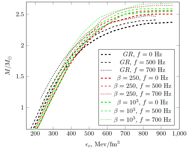
Figure 1: Mass - central density diagram for sequences of stellar configurations with constant frequencies of rotation (for frequency we take $f=500$ and $700$ Hz). Black curves correspond to non-rotating stars.

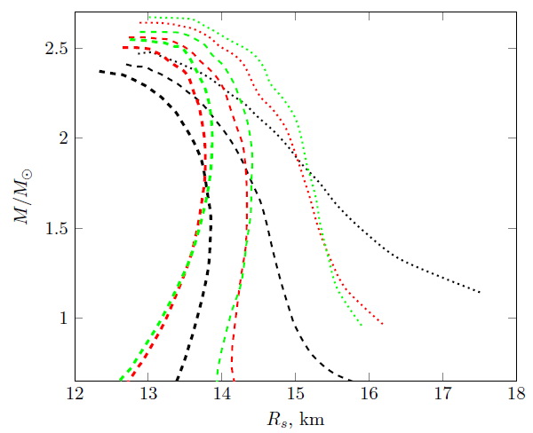
Figure 2: Mass - equatorial radius diagram for same constant frequency sequences as on Fig. 1. The convention of the plot colors and symbols is the same as on Fig. 1.

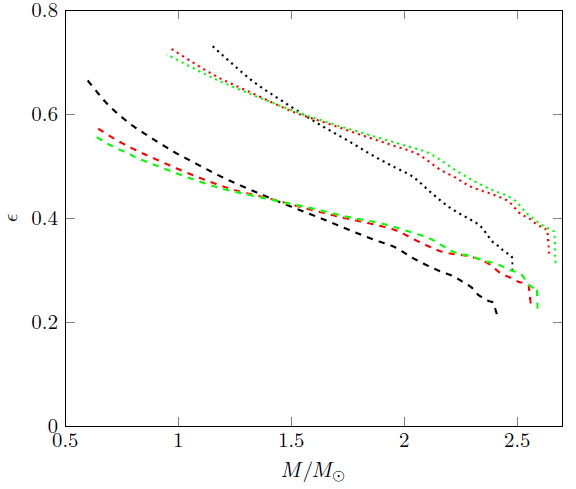
Figure 3: Eccentricity as function of gravitational mass for $f=500$ and $700$ Hz.

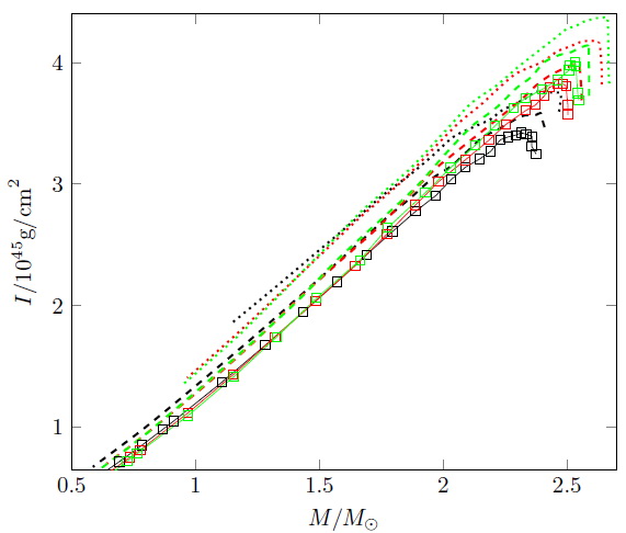
Figure 4: Moment of inertia as function of gravitational mass for nearly static configurations with $f=100$ (squares) and for $f=500$ and $700$ Hz.

$\rho_{c}$, MeV/fm3	230	350	470
GR	735	920	1130
$\alpha=0.25$	745	950	1130
$\alpha=2.5$	770	960	1145
$\alpha=0.25$, $\beta=250$	760	955	1160
$\alpha=0.25$, $\beta=1000$	775	950	1160

Table 1: Keplerian frequency (in Hz) for stellar configurations in General Relativity, pure $R^{2}$ gravity for two values of $\alpha$ and for $R^{2}$ gravity with axions for two values of $\beta$ (with fixed $\alpha=0.25$) at some central densities.

Model	$R_{1.4}^{f=0}$	$R_{1.4}^{f=500}$	$R_{1.4}^{f=700}$
GR	13.82	14.67	16.22
$\alpha=0.25$	13.70	14.47	15.69
$\alpha=2.5$	13.64	14.33	15.43
$\alpha=0.25$, $\beta=250$	13.59	14.33	15.39
$\alpha=0.25$, $\beta=1000$	13.62	14.33	15.38

Table 2: Radii of stellar configurations with $M=1.4M_{\odot}$ for non-rotating case and $f=500$ and $700$ Hz in the same models as in table 1.

Model	$M^{f=0}_{max}$	$M^{f=500}_{max}$	$M^{f=700}_{max}$
GR	2.39	2.43	2.49
$\alpha=0.25$	2.44	2.48	2.53
$\alpha=2.5$	2.51	2.57	2.62
$\alpha=0.25$, $\beta=250$	2.47	2.53	2.58
$\alpha=0.25$, $\beta=1000$	2.53	2.57	2.63

Table 3: Some parameters of neutron stars in the same models as in Table 1: the maximal stable masses in the static case, for frequencies $f=500$ and $700$ Hz.

3 Results

We considered in detail the model of $R^{2}$ gravity with the coupling of axion field $\phi$:

$$F(R,\phi)=R+\alpha R^{2}+\beta{R^{2}\phi}$$ (32)

For axion field we take simple potential without self-interaction following Marsh, 2016

$$V(\phi)=\frac{1}{2}{m^{2}_{a}}\phi^{2}.$$

This assumption corresponds to only small deviations from the potential minimum. For axion mass we assume the value corresponding to Compton wavelength $10r_{g}$ where $r_{g}$ is gravitational radius of Sun ($2.95$ km). For the parameter $\beta$ the range $250<\beta<1000$ in units of $r_{g}^{2}$ is explored. We also compared this model with simple $R^{2}$ gravity without axions and General Relativity.

We fix two parameters (in the case of rotation) for obtaining the stellar configuration, namely central energy density $\rho_{c}$ and angular velocity $\Omega$. Varying central density in given range we obtain sequence of neutron stars rotating with constant angular velocity.

Asymptotical behavior of $A(r,\theta)$ at $r\rightarrow\infty$ defines gravitational mass $M_{s}$ of star for distant observer. In General Relativity the solution of Einstein equations outside the star has the form for non-rotating star:

$$A(r)=\left(1+\frac{M_{s}}{2r}\right)^{2},\quad N(r)=\left(1-\frac{M_{s}}{2r}\right)\left(1+\frac{M_{s}}{2r}\right)^{-1}.$$ (33)

Therefore, the gravitational mass of star can be found as an asymptotical limit

$$M_{s}=2\lim_{r\rightarrow\infty}r(\sqrt{A}-1).$$

One should also account that circumferential radial coordinate ${r_{c}}$ is

$$\tilde{r_{c}}=Ar.$$

Note that in the following the symbol “r” on figures means circumferential radius. Suffix “c” is omitted.

On figure 1 we depicted the gravitational mass-central energy density relations for static case and three values of rotation frequency (for our calculations we considered the cases of $f=100$, $500$ and $700$ Hz). From these diagrams one can see that gravitational mass of star is increased with rotation in our models as in General Relativity.

The mass-equatorial radius diagram for same $f$-constant sequences are depicted on Fig. 2. One need to point out that parameters of stars weakly depend from frequency up to $f\sim 200$ Hz. The same limit is well-known in General Relativity. The interesting problem is to find the limits on masses of fast rotating neutron stars. From observations as well-known fastest rotating pulsar is PSR J1748 - 2446ad with $f=716$ Hz (Hessels, et al., 2006). The minimum mass of a rotating neutron star depends from frequency of rotation and chosen EoS. We can estimate the lower mass of stars with $f=700$ Hz in our model in comparison with General Relativity. From calculations it follows that lower bound for fast rotating neutron stars in our models can be considerably reduced for given EoS. For $f=700$ Hz this limit for $\alpha=0.25$, $\beta=250$ is only $\sim M_{\odot}$ (in General Relativity we have $\sim 1.2M_{\odot}$). For another EoS choice one can expect the same picture: in $R^{2}$ gravity with axions fast rotating stars with smaller masses can exist. From results of Haensel, et al., 2016 and Cipolletta, et al., 2015 it follows that in General Relativity the minimal neutron star masses at $f=716$ Hz for another stiff EoS (NL3, TM1) lie in the range $1.3-1.4M_{\odot}$. In principle the possible future observation of a fast rotating neutron stars with a lower mass could rule out these EoS or could be considered as some indirect confirmation of alternative models of gravity.

Second feature of stellar configurations in $R^{2}$ gravity with axions is that stars with intermediate masses ($1.1M_{\odot}<M<1.4M_{\odot}$) are more compact in comparison with General Relativity (see Table 2). The difference between radii of stars at $700$ Hz is $\sim 1$ km for $M=1.4M_{\odot}$ and up to $2$ km for $M=1.2M_{\odot}$. Therefore in modified gravity one can expect the appearance of more compact fast rotating stars. It is noteworthy that such difference can be tested from observations. X-ray astronomy allows to determine radii of neutron stars with better precision. This effect take place only for fast rotating stars. From Fig. 2 one can see that for static stars the difference between radii is negligible for given interval of masses.

The next question is maximal possible frequency of rotation in our models. Sequence of stellar configurations with given central density will end up at so-called Keplerian frequency $\Omega_{k}$. Hydrostatic equilibrium does not exist for star with $\Omega>\Omega_{k}$ because gravitational force exceeds the centrifugal force at the equator and therefore expulsion of mass from the star begins. This mass-shedding limit on frequency for our model of gravity is higher in comparison with General Relativity. In Table 1 we give the values of Keplerian frequency for some central densities.

In Table 3 we give for comparison some parameters of neutron stars in General Relativity, pure $R^{2}$ gravity (for two values of $\alpha$) and $R^{2}$ gravity with axions for two values of $\beta$ (with fixed $\alpha=0.25$): the maximal stable mass in the static case and for frequencies $f=500$ and $700$ Hz.

Maximal mass of star increases with rotation as expected. Effect of increasing mass due to the coupling between axion field and scalar curvature also is observed. For maximal mass of star with $f=700$ Hz in a case of GM1 EoS we obtained the value $\sim 2.65M_{\odot}$ for $\alpha=0.25$ and $\beta=10^{3}$ in comparison with $M_{max}=2.47M_{\odot}$) in General Relativity. In opposite case of non-rotating stars when difference between radii of stars in modified gravity and General Relativity is $\sim 0.4$ km for $f=500$ and $700$ Hz this quantity is reduced. This occurs because in General Relativity radius of star increases with rotation more strongly in comparison with our model of gravity.

The next interesting question is to investigate the deformation of star caused by rotation. We calculated the eccentricity parameter for stellar configurations as

$$e=\left(1-\frac{R_{p}^{2}}{R_{eq}^{2}}\right)^{1/2}$$ (34)

From Fig. 3 one can see that forms of stellar configurations in our model and in General Relativity in principle are similar for corresponding frequencies.

In description of pulsar properties the main important quantity is the moment of inertia. It can be calculated as

$$I=\frac{J}{\Omega},$$ (35)

where $J$ is angular momentum. For calculation of angular momentum we used the relation from General Relativity namely

$$J=\int_{\Sigma_{t}}(\epsilon+p)UA^{2}B^{2}r^{3}\sin^{2}\theta drd\theta d\phi.$$ (36)

This approximation can be considered as realistic because from the physical viewpoint the inertial characteristics of neutron stars should depend only from solution inside star unlike gravitational mass. Moment of inertia cannot be obtained directly from observations. We depict the moment of inertia as a function of the gravitational mass for frequency constant sequences on Fig. 4 for our model in comparison with General Relativity. Only for masses close to maximal one the inertial moment in modified gravity considerably declines from corresponding value in General Relativity for same frequency. This deviation can affect in principle the evolution of the spin period of massive fast rotating pulsars. Unfortunately we have no a lot of observational data about such pulsars.

One should also note that we considered only one value for axion mass $m_{a}=0.1$ (in units of $r_{g}^{-1}$. In case of non-rotating stars for smaller masses (for example in previous work we considered $m_{a}=0.01$) only size of axion “galo” around the star increases but scalar curvature for $r>50$ km is very close to zero and therefore contribution of term $R\phi^{2}$ is negligible. For stars rotating with frequencies up to $700$ Hz for $r>\sim 20$ km the solution of Einstein equations is very close to static spacetime. Therefore, the rotation parameters of stars weakly depend from parameter $m_{a}$ (of course for $\lambda_{c}>\sim R_{s}$).

4 Conclusion

We investigated realistic model of a uniformly rotating neutron star in axion $R^{2}$ gravity with curvature-axion coupling in the form $\sim R^{2}\phi$. For description of nuclear matter GM1 EoS is used. We calculated gravitational mass, equatorial and polar radii, eccentricity and moment of inertia for stellar configurations with constant frequency.

As in non-rotating case the increase of stellar mass due to axion scalar field takes place for rotating stars and in principle this effect weakly depends from frequency of rotation. One notes also that star radius for our model increases but not significantly for fast rotation. We obtained the increase of mass $\sim 0.2M_{\odot}$ for massive stars in the case of $\beta=1000$. This value is sufficient for possible observational indication of such model. The star radius increases not so considerably ($\sim 100$ m for $\beta=1000$).

Maximal possible frequency of rotation (Keplerian or mass-shedding limit) in $R^{2}$ gravity with axion increases in comparison with General Relativity. Of course this fact is interesting only from theoretical point of view because we have no observational data about compact stars rotating with frequency closed to mass-shedding limit.

However, our results show another interesting (and in principle observable in future) features of stellar configurations in modified gravity with axions. Stars with intermediate masses $M_{\odot}<M<1.4M_{\odot}$ are more compact at the same frequency of rotation. This difference for some parameters ($\sim 1-2$ km) in principle lies in possible errors of radii measurement from NICER mission. Neutron stars in modified gravity in some sense are more stable to fast rotation and mass bound on fast rotating pulsars become lower (for fixed EoS of course). We obtained for GM1 EoS that the limit on mass of fastest rotating neutron star (with $f\sim 700$ Hz) is close to $M_{\odot}$ down $20\%$ than in General Relativity for this EoS. Our preliminary calculations for another realistic EoS (Sly4 and APR) give the similar results. Possible observation of fast, compact stars with relatively small masses could be the best proof of viability of current model of gravity with axions.

Analysis of recently observed GW event (LIGO & Virgo Collaboration, et al., 2020) indicates towards possible existence of neutron stars with mass $2.7M_{\odot}$. This upper limit (if it is reliably confirmed) in combination with constraints on neutron star radii from NICER puts the question about validity of many realistic equations of state for dense matter for example even GM1 EoS considered in paper. In frames of model of $R^{2}$ gravity with axion it is possible to get the increase of observed neutron star masses for required limit for this EoS. It is interesting to consider another modified gravities as well as different interactions between gravity and axions which can lead to increase of maximal mass. We plan to consider this in near future.

Data availability. No new data were generated or analysed in support of this research.

References

- CDMS II Collaboration, et al. (2010) CDMS II Collaboration, et al., 2010, Science, 327, 1619
- LIGO & Virgo Collaboration, et al. (2020) Abbott, R., et al. 2020, arxiv, arXiv:2006.12611
- Alavirad & Weller (2013) Alavirad H., Weller J. M., 2013, PhRvD, 88, 124034
- Alcubierre (2008) Alcubierre M., 2008, Introduction to 3+1 Numerical Relativity, Oxford University Press, Oxford
- Anisimov & Dine (2005) Anisimov A., Dine M., 2005, JCAP, 2005, 009
- (6) Antoniadis J., et al., 2012, MNRAS, 423, 3316
- (7) Antoniadis J., et al., 2013, Science, 340, 448
- Arapoǧlu, Deliduman & Eksi (2011) Arapoǧlu S., Deliduman C., Eksi K. Y., 2011, JCAP, 2011, 020
- Astashenok, Capozziello & Odintsov (2013) Astashenok A. V., Capozziello S., Odintsov S. D., 2013, JCAP, 2013, 040
- Astashenok, Capozziello & Odintsov (2014) Astashenok A. V., Capozziello S., Odintsov S. D., 2014, PhRvD, 89, 103509
- Astashenok, Capozziello & Odintsov (2015) Astashenok A. V., Capozziello S., Odintsov S. D., 2015, Ap&SS, 355, 333
- Astashenok, Capozziello & Odintsov (2015) Astashenok A. V., Capozziello S., Odintsov S. D., 2015, PhLB, 742, 160
- Astashenok, Odintsov & de la Cruz-Dombriz (2017) Astashenok A. V., Odintsov S. D., de la Cruz-Dombriz Á., 2017, CQGra, 34, 205008
- Astashenok, Baigashov & Lapin (2018) Astashenok A. V., Baigashov A.S., Lapin S.A., 2018, Int. J. Geom. Meth. Mod. Phys., 16, 1950004
- Astashenok & Odintsov (2020) Astashenok A.V., Odintsov S.D., 2020, MNRAS, 493 , 78
- Avignone, Creswick & Vergados (2018) Avignone F. T., Creswick R. J., Vergados J. D., 2018, arXiv, arXiv:1801.02072
- Balakin & Ni (2010) Balakin A. B., Ni W.-T., 2010, CQGra, 27, 055003
- Balakin, Bochkarev & Tarasova (2012) Balakin A. B., Bochkarev V. V., Tarasova N. O., 2012, EPJC, 72, 1895
- Balakin, Muharlyamov & Zayats (2014) Balakin A. B., Muharlyamov R. K., Zayats A. E., 2014, EPJD, 68, 159
- Baumgarte & Shapiro (2010) Baumgarte T. W., Shapiro S. L., 2010, Numerical Relativity: Solving Einstein’s Equations on the Computer,
- (21) Bonazzola S., and Maschio G., 1971, Models of Rotating Neutron Stars in General Relativity, in The Crab Nebula, Proceedings from IAU Symposium no. 46, edited by R. D. Davies and F. Graham-Smith, Reidel, Dordrecht, p. 346.
- (22) Bonazzola, S., Gourgoulhon, E., Salgado, M., Marck, J. A. 1993, A&A, 278, 421.
- Bradač, et al. (2008) Bradač M., et al., 2008, ApJ, 687, 959
- Capozziello & Fang (2002) Capozziello S., 2002, IJMPD, 11, 483
- Capozziello, et al. (2011) Capozziello S., de Laurentis M., Odintsov S. D., Stabile A., 2011, PhRvD, 83, 064004
- Capozziello, et al. (2012) Capozziello S., de Laurentis M., de Martino I., Formisano M., Odintsov S. D., 2012, PhRvD, 85, 044022
- Caputo, et al. (2019) Caputo A., Regis M., Taoso M., Witte S. J., 2019, JCAP, 2019, 027
- Caputo, Garay & Witte (2018) Caputo A., Garay C. P., Witte S. J., 2018, PhRvD, 98, 083024
- Caputo (2019) Caputo A., 2019, PhLB, 797, 134824
- Carroll, et al. (2004) Carroll S. M., Duvvuri V., Trodden M., Turner M. S., 2004, PhRvD, 70, 043528
- (31) Chakrabarti S., Delsate T., Gurlebeck N., and Steinhoff J.,2014, PhRvL, 112, 201102
- Cheoun, et al. (2013) Cheoun M.-K., Deliduman C., Güngör C., Keles V., Ryu C. Y., Kajino T., Mathews G. J., 2013, JCAP 2013, 021
- Cicoli, Guidetti & Pedro (2019) Cicoli M., Guidetti V., Pedro F. G., 2019, JCAP, 2019, 046
- Cipolletta, et al. (2015) Cipolletta F., et al., 2015, PhRvD, 92, 023007
- Clowe, et al. (2006) Clowe D., Bradač M., Gonzalez A. H., Markevitch M., Randall S. W., Jones C., Zaritsky D., 2006, ApJL, 648, L109
- (36) Cook G.B., Shapiro S.L., and Teukolsky S.A., 1994, ApJ, 424, 823
- Davis, McCabe & Bœhm (2014) Davis J. H., McCabe C., Bœhm C., 2014, JCAP, 2014, 014
- Davis (2015) Davis J. H., 2015, IJMPA, 30, 1530038
- Day & McDonald (2019) Day F., and McDonald J., 2019, JCAP, 10, 051
- Du, et al. (2018) Du N., et al., 2018, PhRvL, 120, 151301
- Farinelli, et al. (2014) Farinelli R., De Laurentis M., Capozziello S., Odintsov S. D., 2014, MNRAS, 440, 2909
- Feola, et al. (2019) Feola P., Jimenez Forteza X., Capozziello S., Cianci R., Vignolo S., 2019, arXiv, arXiv:1909.08847
- (43) Friedman, J. L., Stergioulas, N., 2013, Rotating Relativistic Stars, Cambridge University Press
- Fukunaga, Kitajima & Urakawa (2019) Fukunaga H., Kitajima N., Urakawa Y., 2019, JCAP, 2019, 055
- Giacomazzo, Rezzolla & Stergioulas (2011) Giacomazzo B., Rezzolla L., Stergioulas N., 2011, PhRvD, 84, 024022
- Giacomazzo & Rezzolla (2011) Giacomazzo, B., Rezzolla, L., 2007, CQGra, 24, 235
- (47) Glendenning N.K., Moszkowski S.A., 1991, PhRvL, 67, 2414
- Gourgoulhon (2007) Gourgoulhon E., 2007, arXiv, gr-qc/0703035
- Gourgoulhon (2010) Gourgoulhon E., 2010, arXiv, arXiv:1003.5015
- (50) Hartle J. B., 1967, ApJ, 150, 1005
- (51) Hartle J. B., Thorne K. S. 1968, ApJ, 153, 807
- Haensel, et al. (2016) Haensel F., et al., 2016, EurPhJA, 52, 59
- Henning, et al. (2018) [ABRACADABRA Collaboration], 2018, DOI: 10.3204/DESY-PROC-2017-02/henning_reyco
- Hessels, et al. (2006) Hessels J. W. T., Ransom S. M., Stairs I. H., et al. 2006, Science, 311, 1901
- Hook & Huang (2018) Hook A., Huang J., 2018, JHEP 18, 36
- Keller & Sedrakian (2013) Keller J., Sedrakian A., 2013, NuPhA, 897, 62
- Khlopov, Sakharov & Sokoloff (1999) Khlopov M. Y., Sakharov A. S., Sokoloff D. D., 1999, NuPhS, 72, 105
- Lawson, et al. (2019) Lawson M., Millar A. J., Pancaldi M., Vitagliano E., Wilczek F., 2019, PhRvL, 123, 141802
- Markevitch, et al. (2003) Markevitch M., et al., 2003, ApJ, 583, 70
- Marsh (2016) Marsh D. J. E., 2016, PhR, 643, 1
- Marsh, et al. (2017) Marsh M. C. D., Russell H. R., Fabian A. C., McNamara B. R., Nulsen P., Reynolds C. S., 2017, JCAP, 2017, 036
- (62) Miller M.C., et al. 2019, ApJL, 887, L24
- Nojiri & Odintsov (2003) Nojiri S., Odintsov S. D., 2003, PhRvD, 68, 123512
- Nojiri, Odintsov & Oikonomou (2017) Nojiri S., Odintsov S. D., Oikonomou V. K., 2017, PhR, 692, 1
- Nojiri & Odintsov (2011) Nojiri S., Odintsov S. D., 2011, PhR, 505, 59
- Odintsov & Oikonomou (2019) Odintsov S. D., Oikonomou V. K., 2019, PhRvD, 99, 104070
- Odintsov & Oikonomou (2019) Odintsov S. D., Oikonomou V. K., 2019, PhRvD, 99, 104070
- Olmo, Rubiera-Garcia & Wojnar (2019) Olmo G. J., Rubiera-Garcia D., Wojnar A., 2019, arXiv, arXiv:1912.05202
- Oppenheimer & Volkoff (1939) Oppenheimer J.R. and Volkoff G.M., 1939, PhRv, 55, 374
- (70) Ostriker J.P. and Mark J. W.-K, 1968, ApJ, 151, 1075
- (71) Pappas G., and Apostolatos T.A., 2012, PhRvL, 108, 231104
- Perlmutter, et al. (1999) Perlmutter S., et al., 1999, ApJ, 517, 565
- Ouellet, et al. (2019) Ouellet J. L., et al., 2019, PhRvL, 122, 121802
- (74) Raaijmakers, G., et al. 2020, ApJL, 893, L21
- Rezzolla, et al. (2018) Rezzolla L., Pizzochero P., Jones D. I., Rea N., Vidaña I., 2018, ASSL..457
- Rezzolla, et al. (2001a) Rezzolla, L., Lamb, F., Markovic, D., Shapiro, S., 2001, PhRvD, 64, 104, 013
- Rezzolla, et al. (2001b) Rezzolla, L., Lamb, F., Markovic, D., Shapiro, S., 2001, PhRvD, 64, 104, 014
- Rezzolla, Lamb & Shapiro (2000) Rezzolla, L., Lamb, F., Shapiro, S., 2000, ApJ 531, L139
- Riess, et al. (1998) Riess A. G., et al., 1998, AJ, 116, 1009
- Riess, et al. (2004) Riess A. G., et al., 2004, ApJ, 607, 665
- Riley, et al. (2019) Riley T. E., et al., 2019, ApJL, 887, L21
- Robertson, Massey & Eke (2017) Robertson A., Massey R., Eke V., 2017, MNRAS, 465, 569
- Roszkowski, Sessolo & Trojanowski (2018) Roszkowski L., Sessolo E. M., Trojanowski S., 2018, RPPh, 81, 066201
- Rozner, et al. (2019) Rozner M., Grishin E., Ginat Y. B., Igoshev A. P., Desjacques V., 2019, arXiv, arXiv:1904.01958
- Safdi, Sun & Chen (2019) Safdi B. R., Sun Z., Chen A. Y., 2019, PhRvD, 99, 123021
- Sakharov & Khlopov (1994) Sakharov A. S., Khlopov M. Y., 1994, PAN, 57, 651
- Sakharov, Sokoloff & Khlopov (1996) Sakharov A. S., Sokoloff D. D., Khlopov M. Y., 1996, PAN, 59, 1005
- Schumann (2019) Schumann M., 2019, JPhG, 46, 103003
- Sedrakian (2016) Sedrakian A., 2016, PhRvD, 93, 065044
- Sedrakian (2019) Sedrakian A., 2019, PhRvD, 99, 043011
- (91) Stergioulas N., & Friedman J. L. 1995, ApJ, 444, 306
- (92) Tolos L., Fabbietti L., 2020, Prog. Part. Nucl. Phys., 112, 103770
- (93) Yagi K., Kyutoku K., Pappas G., Yunes N., and Apostolatos T. A., 2014, PhRvD, 89, 124013
- (94) Yagi K. and Yunes N., 2013, Science 341, 365
- (95) Yagi K. and Yunes N., 2013, PhRvD, 88, 023009