Consequences of Thermal Fluctuations of Well-Known Black Holes in Modified Gravity

Abstract

Quantum fluctuation consequences have significant role in high-energy physics. These fluctuation often regarded as a correction of the infrared (IR) limit. Such correction contribute to the high-energy limit of thermodynamical quantities and the stability conditions of black holes. In this work, we analyze the thermal stability of black holes in the presence of thermal fluctuations. We consider AdS black hole in Born-Infeld massive gravity with non-abelian hair and the charged AdS black hole with a global monopole. We develop many thermodynamical quantities such as entropy, temperature, pressure, heat capacity of a system at constant volume and pressure, ratio between the heat capacities at constant pressure and volume, Gibbs free energy and Helmholtz free energy for both black holes. The critical behavior and phase transitions of black holes are also presented. We also observe the local and global stability of black holes in the grand canonical ensemble and canonical ensemble for the specific values of different parameters, such as, symmetry breaking parameter $\eta$, massive parameter $m$ and non-abelian hair $\nu$.

I Introduction

In GR, black holes (BHs) have shown many generative features of spacetime such as the event horizon, the singularity, Hawking radiation and their connection with thermodynamics. Among all of the above phenomenon, the strong support to the thermodynamical properties of BHs is the Hawking radiation. Classically, nothing can escape from the event horizon of a BH while quantum mechanically it has been proved that BH can emit radiation, known as Hawking radiation 2 -3 and has the Planck spectrum. Discovery of Hawking radiation proved that BHs have temperature, therefore, the concept which is proposed by Bekenstein about the entropy of BHs is no longer a mystery. Also, the incredible work of Hawking made the entropy quantitative which is related to the area of the event horizon $S=\frac{A}{4}$ 4 -5 . The BHs are fluctuating, that is, the event horizon becomes fuzzy because of the quantized metric. Because of the quantum fluctuations, the need of making corrections to the maximum entropy of the BHs has been emerged, which leads towards the development of the holographic principle, which is an emerging new paradigm in quantum gravity 6 -7 . Moreover, the holographic principle implies that the degrees of freedom in a spatial region can be encoded on its boundary, with a density not exceeding one degree of freedom per Planck cell 8 .

Several approaches have been made practical and effective for evaluating the entropy corrections such as by using the non-perturbation quantum general relativity. In this approach the density of microstates for asymptotically flat BHs have been calculated which construct the logarithmic correction to the standard Bekenstein entropy area relation 9 . One can also use the methodologies based on generating logarithmic correction terms for all those BHs whose microscopic degrees of freedom are explained by conformal field theory 10 -11 , Hamiltonian partition functions 12 , loop quantum gravity 13 , near horizon symmetries 14 and thermodynamic arguments 15 . Moreover, the corrections to the entropy of dilation BHs are evaluated which emerged to be the logarithmic corrections 16 . By using the brick wall method, quantum corrections to the entropy of a static spherically symmetric BH global monopole system arising from the Dirac spinor field are investigated in Ref. 17 . The effect of thermal fluctuations for the entropy of both neutral and charged black holes has been investigated in Ref. 18 . Entropy corrections for Schwarzschild BHs has been found by putting it in the center of a spherical cavity of finite radius to achieve equilibrium with surroundings 19 . In a massive theory of gravity, the effects of the quantum fluctuations has been analyzed for a charged BTZ BH in asymptotically AdS and dS spacetimes 20 -21 . The effects of thermal fluctuations on charged ADS BHs and modified Hayward BHs have been investigated in the recent work 22 -23 .

The dRGT model, which is one of the interesting theories of massive gravity is introduced by the de Rham et al. 24 -25 . On the basis of the reference metric, there are various modifications to the dRGT model and Vegh provide one of the good methods 26 and his model undergoes the breaking of the translational symmetry. Zhang and Li proved that this model is stable 27 . After that, the thermodynamical properties and phase transition of many BHs have been investigated 28 -32 . Non-linear electrodynamics (NED) theories are also very useful theories 33 -41 . In order to remove the divergency of self energy of a point-like charge, Born and Infeld introduced one of the best and interesting NED theory which is known as Born-Infeld (BI) theory 42 . In the past few years BI action is being used with the development of superstring theory. D-branes dynamics and some soliton solutions of super-gravity are governed by BI action. For many reasons, extension of RN BH solutions in Einstein-Maxwell theory to charged BH solutions in BI theory along a cosmological constant has attracted some interest in past few years 57 -58 . There are many methods and approaches for studying and exploring the thermal stability and phase transitions of BHs explained in 59 .

Coupled to BI NED, BH solutions and their Van der Waals kind of behavior in massive gravity has been investigated in 44 . In the Maxwell field, one assumes the non-abelian Yang-Mills (YM) field coupled to gravity as a matter source. In Gauss-Bonnet-massive gravity, the thermodynamical properties of BHs and their phase transition in the existence of YM field have been investigated in 45 . In the presence of the YM and BI NED fields, the exact BH solutions of Einstein-Massive theory has been obtained by Hendi and Momennia 46 . After getting motivation from the recent work of Hendi and Momennia 46a , in which they study the thermodynamic description of (a)dS black holes in Born-Infeld massive gravity with a non-abelian hair. We extended their work to discuss the impact of thermal corrections on different parameters of black holes. This paper is outlined as follows: In Sec. II, we concentrate on working out the thermodynamical quantities of the AdS BH in BI massive gravity with a non-abelian hair in the existence of logarithmic correction to entropy. Furthermore, in Sec. III, for the charged AdS BH with a global monopole along with the logarithmic correction to the entropy, we find the conserved and thermodynamical quantities. Sec. IV contains tables of the results and Sec. V is devoted for conclusions.

II AdS Black Hole in BI Massive Gravity with a Non-Abelain Hair

We consider following (3+1)-dimensional action of EYM-massive gravity along with BI NED for the model

$${\L}_{G}=-\frac{1}{16\pi}\int_{M}d^{3+1}x\sqrt{-g}\bigg{(}R-2\Lambda+\ell_{BI}(\digamma_{M})-\digamma_{YM}+m^{2}\sum_{i}c_{i}\emph{U}_{i}(g,f)\bigg{)},$$

where $\ell_{BI}(\digamma_{M})$ and $\digamma_{YM}=\texttt{Tr}(\digamma_{\mu\nu}^{(a)}\digamma^{(a)\mu\nu})$ are the Lagrangian of BI NED and YM invariant, $m$ is related to graviton mass, $f$ make reference to an auxiliary metric, $c_{i}$ and $\emph{U}_{i}$ are free constants and symmetric polynomials of $4\times 4$ matrix $\emph{K}_{\nu}^{\mu}=\sqrt{g^{\mu\sigma}f_{\sigma\nu}}$. We obtain the three tensorial field equations which come from the variation of action of the above equation w.r.t metric tensor $g_{\mu\nu}$, Faraday tensor $F_{\mu\nu}$ and YM tensor $F_{\mu\nu}^{(a)}$, yield as

$$G_{\mu\nu}+\Lambda g_{\mu\nu}=\texttt{T}_{\mu\nu}^{M}+\texttt{T}_{\mu\nu}^{YM}-m^{2}\chi_{\mu\nu},\quad\partial_{\mu}[\sqrt{-g}F^{\mu\nu}\partial_{\digamma}\ell_{BI}(\digamma)]=0,\quad\hat{D}_{\mu}F^{(a)\mu\nu}=0,$$

where $\hat{D}_{\mu}$ is covariant derivative of gauge field. The energy-momentum tensor of electromagnetic and YM fields and $\chi_{\mu\nu}$ is written as

$$\texttt{T}_{\mu\nu}^{M} = \frac{1}{2}g_{\mu\nu}\ell_{BI}(\digamma)-2\digamma_{\mu\nu}\digamma_{\nu}^{\lambda}\partial_{\digamma}\ell_{BI}(\digamma),$$

$$\texttt{T}_{\mu\nu}^{M} = \frac{1}{2}g_{\mu\nu}F_{\rho\sigma}^{(a)}F^{(a)\rho\sigma}+2F_{\mu\lambda}^{(a)}F_{\nu}^{(a)\lambda},$$

$$\chi_{\mu\nu} = -\frac{c_{1}}{2}(\emph{U}_{1}g_{\mu\nu}-\emph{K}_{\mu\nu})-\frac{c_{2}}{2}(\emph{U}_{2}g_{\mu\nu}-2\emph{U}_{1}\emph{K}_{\mu\nu}+2\emph{K}_{\mu\nu}^{2})$$

$$- \frac{c_{3}}{2}(\emph{U}_{3}g_{\mu\nu}-3\emph{U}_{2}\emph{K}_{\mu\nu}+6\emph{U}_{1}\emph{K}_{\mu\nu}^{2}-6\emph{K}_{\mu\nu}^{3})-\cdot\cdot\cdot$$

The exact AdS BH solution of Einstein-Massive theory in the presence of YM and BI NED is being developed by Hendi and Momennia 46 and its line element is given by

$$ds^{2}=-f(r)dt^{2}+\frac{1}{f(r)}dr^{2}+r^{2}(d\theta^{2}+\sin^{2}d\phi^{2}),$$ (1)

where the metric function is

$$f(r)=1-\frac{m_{o}}{r}-\frac{\Lambda r^{2}}{3}+\frac{\upsilon^{2}}{r^{2}}+\frac{m^{2}}{2}(cc_{1}r+2c^{2}c_{2})+\frac{2\beta^{2}r^{2}}{3}(1-\chi_{1}),$$ (2)

and

$$\chi_{1}=_{2}\digamma_{1}(\frac{-1}{2},\frac{-3}{4};\frac{1}{4};\frac{-q^{2}}{\beta^{2}r^{4}}),$$ (3)

which is a hypergeometric function, $\Lambda$ is the cosmological constant, $q$ is the integration constant which is related to the total electric charge of BH, $\nu$ is the magnetic parameter, $c,~{}c_{1}$ and $c_{2}$ are free constants. Also $m_{o}$ is the integration constant which relates with the total mass of BH. The obtained solution possess Coulomb charge, massive term and a non-abelian hair. In the obtained $f(r)$, fourth term $\frac{\nu^{2}}{r^{2}}$ is related to the magnetic charge with non-abelian hair, fifth term is related to the massive gravitons and the last term is related to the non-linearity of electric charge. For massless graviton $m=0$ and linear electrodynamics $\beta\longrightarrow\infty$, $f(r)$ reduces to EYM solution with Maxwell field. By setting $f(r=r_{+})=0$, we have

$$m_{o}=r_{+}-\frac{\Lambda r_{+}^{3}}{3}+\frac{\nu^{2}}{r_{+}}+\frac{m^{2}(cc_{1}r_{{}_{+}}^{2}+2c^{2}c_{2}r_{+})}{2}+\frac{2\beta^{2}r_{+}^{3}(1-\chi_{1})}{3}.$$ (4)

Using the Hamiltonian approach, it was introduced that the total mass $M$ of BH can be obtained by the massive gravity as 47

$$M=\frac{m_{o}}{2}.$$ (5)

Hence, the total mass of BH becomes

$$M=\frac{r_{+}}{2}-\frac{\Lambda r_{+}^{3}}{6}+\frac{\nu^{2}}{2r_{+}}+\frac{m^{2}(cc_{1}r_{+}^{2}+2c^{2}c_{2}r_{+})}{4}+\frac{\beta^{2}r_{+}^{3}(1-\chi_{1})}{3},$$ (6)

which implies that outer horizon $r_{+}\neq 0$. The entropy and volume is related to BH horizon defined as 23

$$S_{o}=\pi r_{+}^{2},~{}~{}V=\frac{4\pi r_{+}^{3}}{3}.$$ (7)

In order to study the thermal fluctuations, thermal stability and phase transitions of BHs, we examine the conserved and thermodynamic quantities such as pressure, entropy, specific heats, Gibbs free energy and Helmholtz free energy of BHs by using the logarithmic correction terms. The temperature of AdS BH in BI massive gravity with non-abelian hair can be written as

$$T=\frac{f^{\prime}(r)}{4\pi}\mid_{r=r_{+}}=\frac{1}{4\pi r_{+}}\bigg{(}1-\Lambda r^{2}_{+}-\frac{\nu^{2}}{r^{2}_{+}}+m^{2}(cc_{1}r_{+}+c^{2}c_{2})+2\beta^{2}r^{2}_{+}\bigg{(}1-\sqrt{1+\frac{q^{2}}{\beta^{2}r^{2}_{+}}}\bigg{)}\bigg{)}.$$ (8)

Now we use the logarithmic correction terms for the entropy in order to discuss the thermal fluctuations. The corrected term for the entropy turns out to be 48

$$S=S_{o}-\frac{b}{2}\log[S_{o}T^{2}],$$ (9)

where $b$ is a constant parameter, which is added in order to handle the logarithmic correction terms produce because of the thermal fluctuations. By setting $b=0$, entropy can be recovered without any correction term.

Using Eqs. (7) and (8) in Eq. (9), we obtain

$$S=\pi r_{+}^{2}-\frac{b}{2}\log\bigg{[}\frac{\bigg{(}1-\Lambda r_{+}^{2}-\frac{\nu^{2}}{r_{+}^{2}}+m^{2}(cc_{1}r_{+}+c^{2}c_{2})+2\beta^{2}r_{+}^{2}\bigg{(}1-\sqrt{1+\frac{q^{2}}{\beta^{2}r_{+}^{2}}}\bigg{)}^{2}}{16\pi}\bigg{]}.$$ (10)

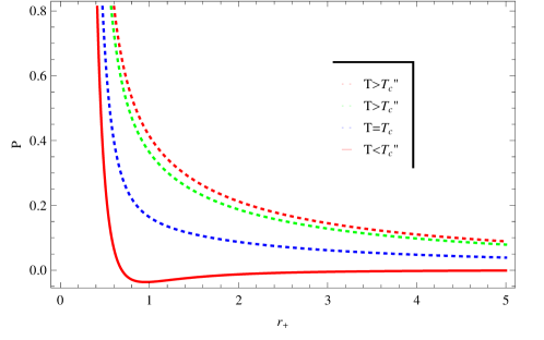
Figure 1: Plot of $P$ versus $r_{+}$ for AdS BH in BI massive gravity with a non-abelain hair. Specific values of different parameters are $\beta=1,~{}\nu=1,~{}c=1$, $m=1$ and $c_{2}=2$.

We consider usual thermodynamical pressure of BHs defined as 66 ,

$$P=\frac{-\Lambda}{8\pi}.$$ (11)

Using Eqs. (8) and (11), one can obtain the equation of state for the considered BH as follow

$$P=-\frac{r^{2}+2\beta^{2}r^{4}-2\beta^{2}\sqrt{1+\frac{q^{2}}{\beta^{2}r^{2}}}r^{4}-4\pi r^{3}T-v^{2}+cm^{2}r^{3}c_{1}+c^{2}m^{2}r^{2}c_{2}}{8\pi r^{4}}.$$ (12)

FIG.1 demonstrates $P$ versus $r_{+}$ for AdS BH in BI massive gravity with a non-abelain hair. The two upper dotted red and green lines correspond to the “ideal gas” phase for $T>T_{c}$, the critical isotherm $T=T_{c}$ is denoted by the dotted blue line, lower solid line corresponds to temperatures smaller than the critical temperature.

II.1 Thermal Stability

In BH thermodynamics, the amount of heat required to change the temperature of a BH, is known as thermal capacity or heat capacity. There are two types of heat capacities, one which measures the specific heat when heat is added to the system at the constant pressure $C_{{}_{p}}$ and the other which measure the specific heat when the heat is added to the system at the constant volume $C_{v}$. We obtain the specific heat at the constant volume by using the following relation

$$C_{v}=T(\frac{\partial S}{\partial r})(\frac{\partial r}{\partial T}).$$ (13)

Using Eqs.(8) and (10), we obtain

$$C_{v} = \frac{-1}{r_{+}\bigg{(}-\frac{4q^{2}}{r_{+}^{4}\sqrt{1+\frac{q^{2}}{\beta^{2}r_{+}^{4}}}}-2\beta^{2}+2\beta^{2}\sqrt{1+\frac{q^{2}}{\beta^{2}r_{+}^{4}}}+\Lambda-\frac{3\nu}{r_{+}^{4}}+\frac{1+c^{2}m^{2}c_{2}}{r_{+}^{2}}\bigg{)}}\bigg{(}1-2r_{+}^{2}\bigg{(}$$ (14)

$$\times -1+\sqrt{1+\frac{q^{2}}{\beta^{2}r_{+}^{4}}}\beta^{2}-r_{+}^{2}\Lambda-\frac{\nu}{r_{+}^{2}}+cm^{2}(r_{+}c_{1}+cc_{2})\bigg{)}\bigg{)}\bigg{(}2\pi r_{+}-\bigg{(}b\bigg{(}4r_{+}\beta^{2}$$

$$- \frac{4r_{+}\beta^{2}}{\sqrt{1+\frac{q^{2}}{\beta^{2}r_{+}^{4}}}}-2r_{+}\Lambda+\frac{2\nu}{r_{+}^{3}}+cm^{2}c_{1}\bigg{)}\bigg{)}\bigg{(}1-2r_{+}^{2}\bigg{(}-1+\sqrt{1+\frac{q^{2}}{\beta^{2}r_{+}^{4}}}\beta^{2}-r_{+}^{2}\Lambda$$

$$- \frac{\nu}{r_{+}^{2}}+cm^{2}(r_{+}c_{1}+cc_{2})\bigg{)}\bigg{)}^{-1}\bigg{)}.$$

The behaviors of heat capacity versus event horizon of the AdS BH in BI massive gravity with a non-abelian hair is displayed in FIGs. 2 and 3. In order to check the local stability of BH, we discuss two cases for fixed values of $m$. When $\Lambda=-1$ and $m=1$, the heat capacity always remain positive and indicates that BH is locally stable and no phase transitions take place. For $m=2$, there occur divergence point at $r_{+}=2.9$ and for $r_{+}<2.9$ BH becomes unstable. While for $r_{+}>2.9$, BH becomes thermodynamically stable. For $m=3$, divergence point occurs at $r_{+}=4.4$ and the phase transitions take place between small BH (SBH) and large BH (LBH). However, BH becomes locally stable for $r_{+}>5.75$, for $\Lambda=1$ and all fixed values of $m$, heat capacity is positive implying that no phase transition will take place and thus, the BH is locally stable for $\Lambda=1$. FIGs.4 and 5 represent the heat capacity versus event horizon of BH for fixed values of $\nu$ for negative and positive cosmological constant. For the case of negative cosmological constant heat capacity is negative for all the fixed values throughout the region which show the local usability of BH. For positive cosmological constant, there are stable and unstable regions depend upon the values of $\nu$, as shown in FIG.5.

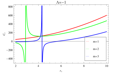
Figure 2: Plot of specific heat versus horizon radius for negative cosmological constant. Specific values of parameters are $\beta=1,~{}\nu=1,~{}c=1,c_{1}=1,c_{2}=1$ and $b=1$

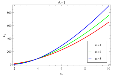
Figure 3: Plot of specific heat versus horizon radius for positive cosmological constant. Specific values of parameters are $\beta=1,~{}\nu=1,~{}c=1,c_{1}=1,c_{2}=1$ and $b=1$

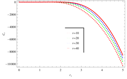
Figure 4: Plot of specific heat versus horizon radius for negative cosmological constant. Specific values of parameters are $\beta=1,~{}c=1,c_{1}=1,c_{2}=1$ and $b=1$

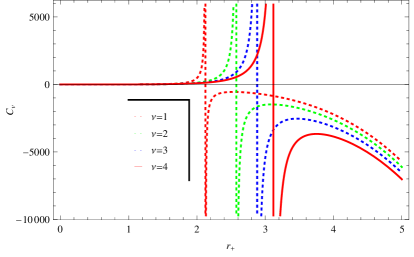
Figure 5: Plot of specific heat versus horizon radius for positive cosmological constant. Specific values of parameters are $\beta=1,~{}c=1,c_{1}=1,c_{2}=1$ and $b=1$

Furthermore, the specific heat at the constant pressure can be evaluated by the following relation

$$C_{p}=\frac{(\frac{\partial M}{\partial r})}{(\frac{\partial T}{\partial r})}.$$ (15)

In view of Eqs. (6) and (10), we have

$$C_{p}=\frac{-2\pi\bigg{(}r_{+}^{2}-r_{+}^{4}(2\beta^{2}(-1+\sqrt{1-\frac{q^{2}}{\beta^{2}r_{+}^{4}}})+\Lambda)-\nu^{2}+cm^{2}r_{+}^{2}(r_{+}c_{1}+cc_{2})\bigg{)}}{r_{+}^{2}\bigg{(}-\frac{4q^{2}}{r_{+}^{4}\sqrt{1+\frac{q^{2}}{\beta^{2}r_{+}^{4}}}}-2\beta^{2}+2\beta^{2}\sqrt{1+\frac{q^{2}}{\beta^{2}r_{+}^{4}}}+\Lambda-\frac{3\nu}{r_{+}^{4}}+\frac{1+c^{2}m^{2}c_{2}}{r_{+}^{2}}\bigg{)}}.$$ (16)

The ratio of the above two heat capacities is also investigated which can be expressed as

$$\gamma=\frac{C_{p}}{C_{v}}.$$ (17)

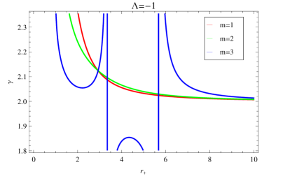
Figure 6: Plot of $\gamma$ versus $r_{+}$ for AdS BH in BI massive gravity with a non-abelian hair for negative cosmological constant. Specific values of different parameters are $\beta=1,~{}\nu=1,~{}c=1,~{}c_{1}=-1,~{}c_{2}=2$ and $b=1$

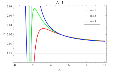
Figure 7: Plot of $\gamma$ versus $r_{+}$ for AdS BH in BI massive gravity with a non-abelian hair for positive cosmological constant. Specific values of parameters are $\beta=1,~{}\nu=1,~{}c=1,~{}c_{1}=-1,~{}c_{2}=2$ and $b=1$

Using Eqs. (14) and (16), we obtain

$$\gamma = \bigg{(}4\pi r_{+}^{2}(q^{2}+r_{+}^{4}\beta^{2})\big{(}-r_{+}^{2}+r_{+}^{4}(2\beta^{2}(-1+\sqrt{1-\frac{q^{2}}{\beta^{2}r_{+}^{4}}})+\Lambda)+\nu^{2}-cm^{2}r_{+}^{2}(r_{+}c_{1}$$

$$+ cc_{2})\big{)}\bigg{)}\bigg{(}-4b\beta^{4}r_{+}^{8}\sqrt{1+\frac{q^{2}}{\beta^{2}r_{+}^{4}}}+2b(q^{2}+r_{+}^{4}\beta^{2})(r^{4}(2\beta^{2}-\Lambda)+\nu)+2\pi r_{+}^{2}(q^{2}+r_{+}^{4}$$

$$+ \beta^{2})\big{(}-r_{+}^{2}+r_{+}^{4}\big{(}2\beta^{2}\big{(}-1+\sqrt{1+\frac{q^{2}}{\beta^{2}r_{+}^{4}}}\big{)}+\Lambda\big{)}+\nu\big{)}+cm^{2}r_{+}^{3}(q^{2}+r_{+}^{4}\beta^{2})\big{(}(b-2$$

$$\times \pi r_{+}^{2})c_{1}-2c\pi r_{+}c_{2}\big{)}\bigg{)}^{-1}.$$

FIGs. 6 and 7 illustrate the behavior of $\gamma$ for $\Lambda=-1$ and $\Lambda=1$ respectively. In the presence of logarithmic correction to the entropy, the value of the $\gamma$ increases for $\Lambda=1$ and decreases for $\Lambda=-1$. When $\Lambda=-1$, the value of $\gamma$ decreases for $m=1$ and $m=2$ while for $m=3$, the values of $\gamma$ has discontinuities. When $\Lambda=1$, the values of $\gamma$ increases for small horizon and then decrease to same values.

II.2 The Gibbs free energy

In order to analyze the global stability of BH, we now treat AdS BH in BI massive gravity with a non-abelian hair as a thermodynamical object by considering it in a grand canonical ensemble. In the grand canonical ensemble free energy is also known as the Gibbs free energy and it is defined as

$$G=M-TS+PV.$$ (19)

Inserting Eqs. (6), (7), (8), (10) and (12) into (19), we get

$$G = r_{+}-\frac{r_{+}^{3}\Lambda}{3}+\frac{\nu^{2}}{r_{+}}-\frac{2r_{+}^{3}\beta^{2}}{3}\bigg{(}-1+_{2}\digamma_{1}\big{(}\frac{-1}{2},\frac{-3}{4};\frac{1}{4};\frac{-q^{2}}{\beta^{2}r_{+}^{4}}\big{)}\bigg{)}+\frac{1}{2}cm^{2}r_{+}\big{(}r_{+}c_{1}+2cc_{2}\big{)}$$ (20)

$$+ \bigg{(}\frac{1}{8\pi r_{+}^{3}}\bigg{)}\times\bigg{(}2\pi r_{+}^{2}+b\log[16\pi]-b\log[\bigg{(}-1+2r_{+}^{2}\beta^{2}\bigg{(}-1+\sqrt{1+\frac{q^{2}}{r_{+}^{4}\beta^{2}}}\bigg{)}+r_{+}^{2}\Lambda$$

$$+ \frac{\nu}{r_{+}^{2}}-cm^{2}(r_{+}c_{1}+cc_{2})\bigg{)}^{2}]\bigg{)}\bigg{(}-r_{+}^{2}+r_{+}^{4}\bigg{(}2\beta^{2}\bigg{(}-1+\sqrt{1+\frac{q^{2}}{r_{+}^{4}\beta^{2}}}\bigg{)}+\Lambda\bigg{)}$$

$$+ \nu-cm^{2}r_{+}^{2}(r_{+}c_{1}+cc_{2})\bigg{)}-\frac{r^{3}}{6}((-12Mr+6r^{2}+6v^{2}+4r^{4}\beta^{2}-4r^{4}\chi_{1}\beta^{2}+3c$$

$$\times m^{2}r^{3}c_{1}+6c^{2}m^{2}r^{2}c_{2})(2r^{4})^{-1})$$

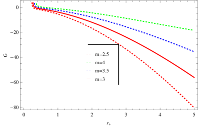
Figure 8: Plot of Gibbs free energy versus $r_{+}$ for AdS BH in BI massive gravity with a non-abelian hair for negative cosmological constant. Specific values of parameters are $\beta=1,~{}\nu=1,~{}c=1,~{}c_{1}=1,~{}c_{2}=2$ and $b=1$

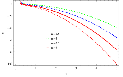
Figure 9: Plot of Gibbs free energy versus $r_{+}$ for AdS BH in BI massive gravity with a non-abelian hair for positive cosmological constant. Specific values of parameters are $\beta=1,~{}\nu=1,~{}c=1,~{}c_{1}=1,~{}c_{2}=2$ and $b=1$

The graphical representation of the Gibbs free energy and the horizon radius for the fixed values of massless graviton and cosmological constant takes place in the FIGs. 8 and 9. The left panel is for $\Lambda=-1$, while right panel is for $\Lambda=1$, one can see that the Gibbs free energy is negative throughout the region for both the cases. Gibbs free energy is used to discuss the global stability of BH. The negative trajectories for both the mentioned cases for all the values of $m$ represent the unstable region.

II.3 Canonical ensemble

If the transference of charge on the BH is restrained then the BH could be regarded as a thermodynamically closed system such as a conical ensemble. When the charge is fixed, the free energy is known as the Helmholtz free energy in the canonical ensemble and its expression can be derived by using the following relation

$$F=G-PV.$$ (21)

By using Eq. (20), the Helmholtz free energy for AdS BH in BI massive gravity with a non-abelain hair can be obtained as

$$F = r_{+}-\frac{r_{+}^{3}\Lambda}{3}+\frac{\nu^{2}}{r_{+}}-\frac{2r_{+}^{3}\beta^{2}}{3}\bigg{(}-1+_{2}\digamma_{1}\big{(}\frac{-1}{2},\frac{-3}{4};\frac{1}{4};\frac{-q^{2}}{\beta^{2}r_{+}^{4}}\big{)}\bigg{)}+\frac{1}{2}cm^{2}r_{+}\big{(}r_{+}c_{1}+2cc_{2}\big{)}$$ (22)

$$+ \bigg{(}\frac{1}{8\pi r_{+}^{3}}\bigg{)}\bigg{(}2\pi r_{+}^{2}+b\log[16\pi]-b\log\bigg{[}\bigg{(}-1+2r_{+}^{2}\beta^{2}\bigg{(}-1+\sqrt{1+\frac{q^{2}}{r_{+}^{4}\beta^{2}}}\bigg{)}+r_{+}^{2}\Lambda$$

$$+ \frac{\nu}{r_{+}^{2}}-cm^{2}(r_{+}c_{1}+cc_{2})\bigg{)}^{2}\bigg{]}\bigg{)}\bigg{(}-r_{+}^{2}+r_{+}^{4}\bigg{(}2\beta^{2}\bigg{(}-1+\sqrt{1+\frac{q^{2}}{r_{+}^{4}\beta^{2}}}\bigg{)}+\Lambda\bigg{)}+\nu-cm^{2}$$

$$\times r_{+}^{2}(r_{+}c_{1}+cc_{2})\bigg{)}+(16\pi^{2}r_{+}^{3})\bigg{(}3\bigg{(}-\frac{4q^{2}}{r_{+}^{4}\sqrt{1+\frac{q^{2}}{\beta^{2}r_{+}^{4}}}}-2\beta^{2}+2\beta^{2}\sqrt{1+\frac{q^{2}}{\beta^{2}r_{+}^{4}}}+\Lambda-\frac{3\nu}{r_{+}^{4}}$$

$$+ \frac{1+c^{2}m^{2}c_{2}}{r_{+}^{2}}\bigg{)}\bigg{)}^{-1}.$$

Figure 10: Plot of Gibbs free energy versus $r_{+}$ for AdS BH in BI massive gravity with a non-abelian hair for negative cosmological constant. Specific values of parameters are $~{}\nu=1,~{}c=1,~{}c_{1}=1,~{}c_{2}=2$ and $b=1$

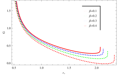
Figure 11: Plot of Gibbs free energy versus $r_{+}$ for AdS BH in BI massive gravity with a non-abelian hair for positive cosmological constant. Specific values of parameters are $~{}\nu=1,~{}c=1,~{}c_{1}=1,~{}c_{2}=2$ and $b=1$

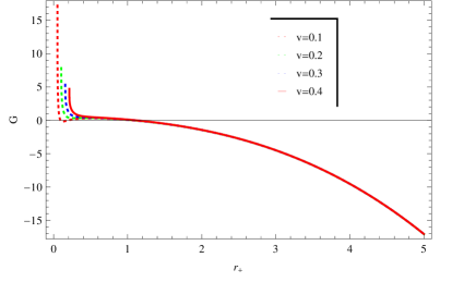
Figure 12: Plot of Gibbs free energy versus $r_{+}$ for AdS BH in BI massive gravity with a non-abelian hair for negative cosmological constant. Specific values of parameters are $\beta=1,~{}c=1,~{}c_{1}=1,~{}c_{2}=2$ and $b=1$

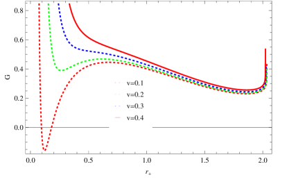
Figure 13: Plot of Gibbs free energy versus $r_{+}$ for AdS BH in BI massive gravity with a non-abelian hair for positive cosmological constant. Specific values of parameters are $\beta=1,~{}c=1,~{}c_{1}=1,~{}c_{2}=2$ and $b=1$

In FIGs. 10 and 11, we study the impact of non-linear electrodynamics on the Gibbs free energy of AdS BH in BI massive gravity with non-abelian hair. While in FIGS. 12 and 13, we demonstrate the impact of non-abelian hair on the Gibbs free energy. In FIGs. 10 and 12, non-linear electrodynamics and non-abelian hair effect slightly on the Gibbs free energy. For very smaller values of horizon radius, Gibbs free energy is positive while it becomes negative for increasing values of $r_{+}$. The impact of non-linear electrodynamics and non-abelian hair for the case of positive cosmological constant in FIGs. 11 and FIGS. 13 are remarkable because it makes the Gibbs energy positive. There is only one case $\nu=0.1$ for which Gibbs energy is negative for very small interval of horizon radius.

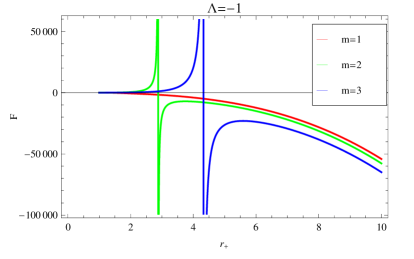
Figure 14: Plot of Helmholtz free energy versus $r_{+}$ for AdS BH in BI massive gravity with a non-abelian hair for negative cosmological constant. Specific values of parameters are $\beta=1,~{}\nu=1,~{}c=1,~{}c_{1}=-1,~{}c_{2}=2$ and $b=1$

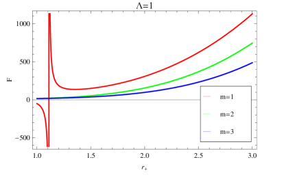
Figure 15: Plot of Helmholtz free energy versus $r_{+}$ for AdS BH in BI massive gravity with a non-abelian hair for positive cosmological constant. Specific values of parameters are $\beta=1,~{}\nu=1,~{}c=1,~{}c_{1}=-1,~{}c_{2}=2$ and $b=1$

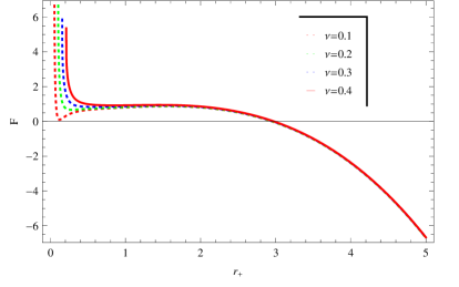
Figure 16: Plot of Helmholtz free energy versus $r_{+}$ for AdS BH in BI massive gravity with a non-abelian hair for negative cosmological constant. Specific values of parameters are $\beta=1,m=1,~{}c=1,~{}c_{1}=-1,~{}c_{2}=2$ and $b=1$

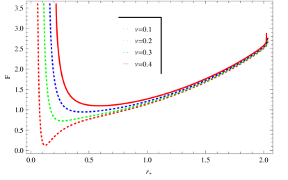
Figure 17: Plot of Helmholtz free energy versus $r_{+}$ for AdS BH in BI massive gravity with a non-abelian hair for positive cosmological constant. Specific values of parameters are $\beta=1,m=1,~{}c=1,~{}c_{1}=-1,~{}c_{2}=2$ and $b=1$

Behavior of the Helmholtz free energy $F$ against the horizon radius $r_{+}$ is represented in the FIGs.14 and 15 for both positive and negative cosmological constant at fixed values of massless graviton. When $\Lambda=-1$, for $m=1$ the Helmholtz free energy decreases and becomes negative for the larger horizon. When $m=2$, the Helmholtz free energy is positive for SBH but becomes negative when $r_{+}\geq 2.8$. When $m=3$, the Helmholtz free energy becomes negative for $r_{+}\geq 4.3$. We conclude that the Helmholtz free energy is negative for the larger horizon and higher values of massless graviton for the negative cosmological constant. When $\Lambda=1$, for $m=1$ the Helmholtz free energy is negative for small horizon while for $r\geq 1.1$, Helmholtz free energy becomes positive. For $m=2$ and $m=3$, the Helmholtz free energy is positive and increases for the larger values of horizon radius. We conclude that, the Helmholtz free energy is higher for $m=1$ as compared with $m=2$ and $m=3$. Also the Helmholtz free energy is positive, which leads to stability for the larger horizon radius and positive cosmological constant. FIGs. 16 and 17 demonstrate Helmholtz free energy for positive and negative cosmological constant at fixed values of $\nu$. For the case of negative cosmological constant Helmholtz energy is positive for very small horizon radius of all fixed values of $\nu$, then it turns to negative for intermediate and large horizon. For positive cosmological constant, Helmholtz energy is positive for all the cases of $\nu$.

III Charged AdS BH With a Global Monopole

The gravitational field of a global monopole which is an approximate solution for the metric outside a monopole produce from the breaking of a $O(3)$ symmetry is discussed by Barriola and Vilenkin 51 . When a charged AdS BHs swallows a global monopole the general static spherically symmetric metric and gauged potential can be written as 52

$$d\tilde{s}^{2}=-\tilde{f}{\tilde{(r)}}d\tilde{t}^{2}+\frac{1}{\tilde{h}{\tilde{(r)}}}+\tilde{r}^{2}(d\theta^{2}+sin^{2}\theta d\phi^{2}),$$ (23)

$$\tilde{A}=\frac{\tilde{q}}{\tilde{r}}d\tilde{t},~{}~{}\tilde{f}{(\tilde{r})}=\tilde{h}{(\tilde{r})}=1-8\pi\eta_{o}^{2}-\frac{2\tilde{m}}{\tilde{r}}+\frac{\tilde{q}^{2}}{\tilde{r}^{2}}+\frac{\tilde{r}^{2}}{l^{2}},$$ (24)

where $\tilde{m}$ is the mass parameter and $\tilde{q}$ is an electric charge parameter. Also, $l$ is associated with the cosmological constant as $\Lambda=-\frac{3}{l^{2}}$. The coordinate transformations are given by

$$\tilde{t}=(1-8\pi\eta_{o}^{2})^{-\frac{1}{2}}t,\tilde{r}=(1-8\pi\eta_{o}^{2})^{\frac{1}{2}}r.$$ (25)

New parameters can be defined as follows

$$m=(1-8\pi\eta_{o}^{2})^{-\frac{3}{2}}\tilde{m},q=(1-8\pi\eta_{o}^{2})^{-1}\tilde{q},\eta^{2}=8\pi\eta_{o}^{2},$$ (26)

where $\eta$ is the symmetry breaking parameter. In view of Eqs. (23) and (25), Eq. (26) can be written as,

$$ds^{2}=-f(r)dt^{2}+\frac{1}{h(r)}dr^{2}+(1-\eta^{2})r^{2}(d\theta^{2}+sin^{2}\theta d\phi^{2}),$$ (27)

the solution will take the form of the four-dimensional Reissner-Nordst$\ddot{o}$m (RN) AdS BH if we set $\eta=0$, where

$$A=\frac{q}{r}dt,f(r)=h(r)=1-\frac{2m}{r}+\frac{q^{2}}{r^{2}}+\frac{r^{2}}{l^{2}},$$ (28)

by using $l^{2}=-\frac{3}{\Lambda}$, we get

$$f(r)=1-\frac{2m}{r}+\frac{q^{2}}{r^{2}}-\frac{\Lambda r^{2}}{3}.$$ (29)

In order to calculate the thermodynamical quantities of charged AdS BH with global monopole, we begin with the event horizon of the BH situated at $r=r_{h}$, which is the largest root of the $f(r)=h(r)=0$. At infinity, the electric charge $q$ along with the potential can be evaluated by

$$Q=\frac{1}{4\pi}\oint\textsl{F}^{\mu\omega}d^{2}\sum{\mu\omega}=(1-\eta^{2})q,$$ (30)

$$\Phi=\xi^{\mu}A_{\mu}|_{r=r_{h}}=\frac{q}{r_{h}},$$ (31)

where $\xi^{\mu}$ is the timelike killing vector $(\partial_{t})^{\mu}$ 53 . The Arnowitt-Deser-Misner (ADM) mass $M$ of the system can be evaluated by the Komar integral

$$M=\frac{1}{8\pi}\oint\xi_{(t)}^{\mu:\nu}d^{2}\sum_{\mu\nu},$$ (32)

$$M=(1-\eta^{2})m.$$ (33)

In order to find the expression for mass put $f(r)=0$ in Eq. (29), we obtain

$$m=\frac{r}{2}+\frac{q^{2}}{2r}-\frac{\Lambda r^{3}}{6}.$$ (34)

By using Eqs. (30), (33) and (34), we get

$$M=(1-\eta^{2})\bigg{(}\frac{r_{+}}{2}+\frac{Q^{2}}{(1-\eta^{2})^{2}2r_{+}}-\frac{\Lambda r_{+}^{3}}{6}\bigg{)}.$$ (35)

The Hawking temperature $T$ of the charged AdS BH with global monopole is given by

$$T=\frac{f^{\prime}(r)}{4\pi}=\frac{1}{4\pi r_{+}}\bigg{(}1-\Lambda r_{+}^{2}-\frac{Q^{2}}{(1-\eta^{2})^{2}r_{+}^{2}}\bigg{)}.$$ (36)

The area $A$ at the horizon of the charged AdS BH with golobal monopole can be obtained as

$$A=\int_{r=r_{+}}\sqrt{g_{\theta\theta}g_{\phi\phi}}d\theta d\phi=4\pi(1-\eta^{2})r_{+}^{2}.$$ (37)

The entropy $S_{o}$ can be evaluated by using the above equation is given by

$$S_{o}=\frac{A}{4}=\pi(1-\eta^{2})r_{+}^{2}.$$ (38)

The logarithmic correction term for the entropy of charged AdS BH with global monopole can be obtained by using Eq. (9)

$$S=\pi(1-\eta^{2})r_{+}^{2}-\frac{b}{2}\log\bigg{[}\frac{(1-\eta^{2})\bigg{(}1+\frac{Q^{2}}{r_{+}^{2}(-1+\eta^{2})^{2}}-r_{+}^{2}\Lambda\bigg{)}^{2}}{16\pi}\bigg{]}.$$ (39)

The thermodynamic volume $V=(\frac{\partial M}{\partial P})$ can be given as

$$V=\frac{4\pi(1-\eta^{2})r_{+}^{3}}{3}.$$ (40)

From the above results, it is clear that the thermodynamical quantities such as, the electric charge $Q$, the ADM mass $M$, the area at the horizon of the BH $A$, the thermodynamic volume $V$, the corrected term of the entropy $S$ and the temperature $T$ are associated with the the symmetry breaking parameter $\eta$. The first law of thermodynamics holds for the above thermodynamical quantities for details see ref a100 . We step forward to analyze the thermal stability, phase transition, local and global stability in the presence of the grand canonical ensemble and canonical ensemble. The equation of state for charged AdS BH with global monopole take the following form

$$P=\frac{Q^{2}+\left(-1+\eta^{2}\right)^{2}r^{2}(-1+4\pi rT)}{8\left(-1+\eta^{2}\right)^{2}\pi r^{4}}.$$ (41)

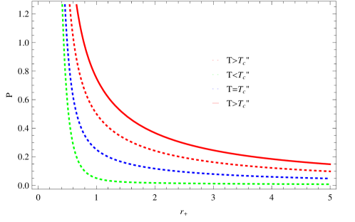
Figure 18: Plot of $P$ versus $r_{+}$ for charged AdS BH with a global monopole.

FIG. 18 demonstrates $P$ versus $r_{+}$ for charged AdS BH with a global monopole. The two upper red lines correspond to the “ideal gas” phase for $T>T_{c}$, the critical isotherm $T=T_{c}$ is denoted by the dotted blue line, lower dotted green correspond to temperatures smaller than the critical temperature.

Further, to analyze and study the phase transition of the charged AdS BH with a global monopole, we move to evaluate the important thermodynamical quantities such as the heat capacities $C_{p}$ and $C_{v}$. Generally, when the heat capacity is positive it implies that the BH is stable and negative heat capacity implies that BH is unstable. Instability of a BH means that the BH cannot bear even a small perturbation and proceed to disappear. Heat capacity for the mentioned BH can be evaluated by the using the relation Eq. (13) as

$$C_{v} = \frac{1}{3Q^{2}-r_{+}^{2}(-1+\eta^{2})^{2}(1+r_{+}^{2}\Lambda)}\times\bigg{(}r_{+}^{3}(-1+\eta^{2})^{2}\big{(}1-\frac{Q^{2}}{r_{+}^{2}(-1+\eta^{2})^{2}}-r_{+}^{2}\Lambda\big{)}$$

$$\times \big{(}-2\pi r_{+}(-1+\eta^{2})+\frac{2b(Q^{2}+r_{+}^{4}(-1+\eta^{2})^{2}\Lambda)}{r_{+}(Q^{2}-r^{2}(-1+\eta^{2})^{2}(-1+r_{+}^{2}\Lambda))}\big{)}\bigg{)}.$$

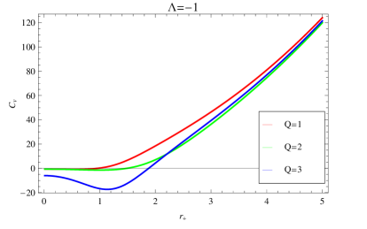
Figure 19: Plot of $C_{v}$ versus $r{+}$ for charged AdS BH with a global monopole for negative cosmological constant.

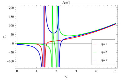
Figure 20: Plot of $C_{v}$ versus $r_{+}$ for charged AdS BH with a global monopole for positive cosmological constant.

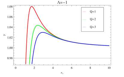
Figure 21: Plot of $\gamma$ versus $r_{+}$ for charged AdS BH with a global monopole for negative cosmological constant.

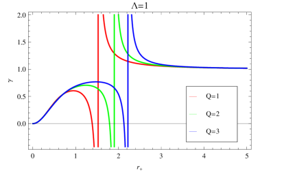
Figure 22: Plot of $\gamma$ versus $r_{+}$ for charged AdS BH with a global monopole for positive cosmological constant.

The graphical analysis of heat capacity at constant volume is represented in FIGs. 19 and 20 for negative and positive cosmological constant respectively. In Fig. 19, when $\Lambda=-1$, the $C_{v}$ is negative for $0\leq r_{+}\leq 0.1,~{}0\leq r_{+}\leq 1.5$ and $0\leq r_{+}\leq 1.89$ for $Q=1,~{}Q=2$ and $Q=3$, respectively. The heat capacity is positive for higher values of horizon radius. We conclude that, for negative cosmological constant, phase transition takes place and BH is unstable for lower values of horizon radius but stable for larger values of horizon radius. In FIG. 20, when $Q=1$, the curve has two regions with one divergent point. The small radius region has negative heat capacity therefore BH is unstable in this region while the large radius region has positive heat capacity therefore it is stable. When $Q=2$, the curve has four regions with three divergent points. For the small horizon, the heat capacity is negative and thus it is unstable. For the first part of the intermediate part of the horizon, the heat capacity is positive and BH is stable in this region. But in the second part of the intermediate BH (IBH) the heat capacity is negative and so BH is unstable. The LBH has positive heat capacity and therefore BH is stable in this region. The phase transition takes place in between SBH first and second part of IBH and LBH. When $Q=3$, the curve has two divergent points in three regions. The phase transition takes place again as shown in the figure.

Now, the heat capacity when the heat is added to the system at the constant pressure $C_{P}$ can be evaluated by the using the relation Eq.(15) as

$$C_{p}=-\frac{2\pi r_{+}^{2}(-1+\eta^{2})(Q^{2}+r_{+}^{2}(-1+\eta^{2})^{2}(-1+r_{+}^{2}\Lambda))}{-3Q^{2}+r_{+}^{2}(-1+\eta^{2})^{2}(1+r_{+}^{2}\Lambda)}$$ (43)

Also, $\gamma$ turns out to be

$$\gamma = \bigg{(}\pi r_{+}^{2}(-1+\eta^{2})(-Q^{2}+r_{+}^{2}(-1+\eta^{2})^{2}(-1+r^{2}\Lambda))\bigg{)}\bigg{(}b(Q^{2}+r_{+}^{4}(-1+\eta^{2})^{2}\Lambda)$$

$$- \pi r_{+}^{2}(-1+\eta^{2})(Q^{2}+r_{+}^{2}(-1+\eta^{2})^{2}(1-r_{+}^{2}\Lambda))\bigg{)}^{-1}.$$

FIGs. 21 and 22 represent the graphical analysis on $\gamma$ versus $r_{+}$ for negative and positive cosmological constant, respectively. In FIG. 21 for $\Lambda=-1$, $\gamma$ is higher for the lower values of $Q$. For $Q=1,~{}Q=2$ and $Q=3$, the values of $\gamma$ are highest at $r_{+}=1.6,~{}r_{+}=2.5$ and $r_{+}=3$, respectively. For $r_{+}\geq 5$, the value of $\gamma$ starts approaching to the same value for all different values of $Q$. We conclude that for the negative cosmological constant and for all different values of $Q$, the values of $\gamma$ are positive. In FIG. 22, we analyze the graph for three different values of $Q$ and discuss the case for $\Lambda=1$. When $Q=1$, for the small radial region, $\gamma$ is positive for the first part of the intermediate region then $\gamma$ becomes negative and again for the second part of intermediate region for large radial region, $\gamma$ becomes positive. When $Q=1$ and $Q=2$, both curves show similar behavior as per $Q=1$. Hence, we conclude that the for the smaller values of radius, the $\gamma$ is negative while for the larger values of the radius, the $\gamma$ is positive and the curve approaches to the same value of $\gamma$.

Now, we investigate the global stability of the charged AdS BH with a global monopole by using the Gibbs free energy or free energy in the grand canonical ensemble. The Gibbs free energy can be derived by using Eq.(19). The expression for the Gibbs free energy of the charged AdS BH with global monopole is

$$G = \frac{1}{24(-1+\eta^{2})^{2}r^{3}}(12(-1+\eta^{2})r^{2}(Q^{2}+(-1+\eta^{2})r(2M+(-1+\eta^{2})r))+4(-1$$

$$+ \eta^{2})r^{2}(-3Q^{2}+(-1+\eta^{2})^{2}r^{2}(-3+\Lambda r^{2}))-(3(Q^{2}+(-1+\eta^{2})^{2}r^{2}(-1+\Lambda r^{2}))$$

$$\times (2(-1+\eta^{2})\pi r^{2}+b\text{Log}[\frac{(1-\eta^{2})(1+\frac{Q^{2}}{(-1+\eta^{2})^{2}r^{2}}-\Lambda r^{2})^{2}}{16\pi}]))(\pi)^{-1})$$

FIGs. 23 and 24 depict the graph between the Gibbs free energy $G$ against the radius of the BH at the horizon $r_{+}$ at different values of $Q$. In FIG. 23, when $\Lambda=-1$, apparently there are no divergent points. In the small region radius, the Gibbs free energy is negative for all different values of $Q$. But the Gibbs free energy is positive and displays a smooth curve in the IBH and again its negative in the LBH. Thus, we conclude that the charged AdS BH with a global monopole is unstable in the SBH and LBH but, its stable in the IBH. In FIG. 24, for all different values of $Q$, the Gibbs free energy is negative for the SBH and positive for the LBH. When $Q=4$, the Gibbs free energy is highest as compared to for the $Q=3$, $Q=2$ and $Q=1$. Thus, the Gibbs free energy is higher for the higher the value of $Q$. We conclude that the charged AdS BH with a global monopole is globally stable for the larger horizon radius.

Now, for investing the thermodynamically global stability in the canonical ensemble, we will consider the charged AdS BH with a global monopole in the canonical ensemble. The free energy or the Helmholtz free energy for charged AdS BH with a global monopole can be derived by using the Eq. (21) as

$$F = \frac{1}{24}\bigg{(}\frac{4(-1+\eta^{2})(-3(q^{2}+r_{+}^{2})+r_{+}^{4}\Lambda)}{r_{+}}-\frac{1}{\pi}\bigg{(}2(1-\frac{Q^{2}}{r_{+}^{2}(-1+\eta^{2})^{2}}-r_{+}^{2}\Lambda)(-2\pi r_{+}(-1$$ (46)

$$+ \eta^{2})+\frac{2b(Q^{2}+r_{+}^{4}(-1+\eta^{2})^{2}\Lambda)}{r_{+}(Q^{2}-r_{+}^{2}(-1+\eta^{2})^{2}(-1+r_{+}^{2}\Lambda))})\bigg{)}-\frac{1}{\pi r_{+}^{3}(-1+\eta^{2})^{2}}\bigg{(}3(Q^{2}+r_{+}^{2}(-1+\eta^{2})^{2}$$

$$\times (-1+r_{+}^{2}\Lambda))(2\pi r_{+}^{2}(-1+\eta^{2})$$

$$+ b\log[\frac{(1-\eta^{2})(-1+\frac{Q^{2}}{r_{+}^{2}(-1+\eta^{2})^{2}}+r_{+}^{2}\Lambda)}{16\pi}])\bigg{)}\bigg{)}.$$

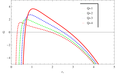
Figure 23: Plot of $G$ versus $r_{+}$ for charged AdS BH with a global monopole for negative cosmological constant.

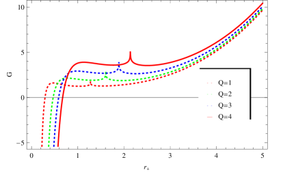
Figure 24: Plot of $G$ versus $r_{+}$ for charged AdS BH with a global monopole for positive cosmological constant.

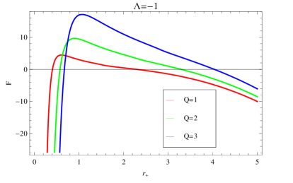
Figure 25: Plot of $F$ versus $r_{+}$ for charged AdS BH with a global monopole for negative cosmological constant.

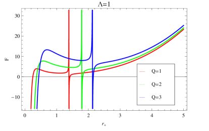
Figure 26: Plot of $F$ versus $r_{+}$ for charged AdS BH with a global monopole for positive cosmological constant.

The graphical analysis of Helmholtz free energy for charged AdS BH with a global monopole for specific values of different parameters is represented in the FIGs. 25 and 26. In FIG. 25, for $Q=1,~{}Q=2$ and $Q=3$, when the cosmological constant is negative the Helmholtz free energy is positive for $0.25\leq r_{+}\leq 1.5,~{}0.6\leq r_{+}\leq 2.25$ and $0.65\leq r_{+}\leq 2.8$, respectively. The Helmholtz free energy is negative for the larger horizon radius thus the charged AdS BH with a global monopole is unstable for LBH. In FIG. 26, for $\Lambda=1$, Helmholtz free energy displays an interesting and yet complicated behavior. For $Q=1$, the Helmholtz free energy is negative for the SBH but it is positive for the IBH and LBH. Similarly, for $Q=2$ and $Q=3$, the Helmholtz free energy is negative for the SBH and positive for the IBH and LBH. The Helmholtz free energy is increasing and stays positive for the larger horizon radius. The Helmholtz free energy is higher for the higher values of $Q$. Thus, we conclude that for the lower horizon radius the charged AdS BH with a global monopole is globally unstable and for the higher horizon radius it is globally stable.

Our purpose was to check that does presence of monopole has any influence on the phase behavior of the charged AdS BH with global monopole. The above calculations and the graphical representation implies that the charged AdS BH with a global monopole undergo a small to large BH phase transition which is remarkably explained through the graphical representation in FIGs. 19-26. Until now, we have analyzed and discussed the local thermodynamical properties of the charged AdS BH with a global monopole. We have find that the charged AdS BH with a global monopole experiences a SBH and LBH phase transition, which is interestingly remarkable. If we compare our results with RN AdS BH, we can easily see that the existence of the global monopole has influence on the critical points but the law of corresponding states remain unchanged and constant as stated above.

III.1 Tables

Table 1: Summary table for the heat capacity $C_{v}$ versus $r_{+}$ for $\Lambda=-1$ and $\eta=0.5$.

$C_{v}$	$Q$	Horizon radius $r_{+}$	Stability
	Q=1	$0\leq r_{+}\leq 0.1$	unstable
negative	$Q=2$	$0\leq r_{+}\leq 1.5$	unstable
	$Q=3$	$0\leq r_{+}\leq 1.89$	unstable
	$Q=1$	$r_{+}=0.11$	Phase Transition
$C_{v}=0$	$Q=2$	$r_{+}=0.51$	Phase Transition
	$Q=3$	$r_{+}=0.91$	Phase Transition
	$Q=1$	$r_{+}\geq 0.12$	stable
positive	$Q=2$	$r_{+}\geq 0.52$	stable
	$Q=3$	$r_{+}\geq 0.2$	stable

Table 2: Summary table for the heat capacity $C_{v}$ versus $r_{+}$ for $\Lambda=1$ and $\eta=0.5$.

$C_{v}$	$Q$	Horizon radius $r_{+}$	Stability
	Q=1	$0\leq r_{+}\leq 1.26,~{}1.41\leq r_{+}\leq 1.44$	unstable
negative	$Q=2$	$0\leq r_{+}\leq 1.28,~{}2.15\leq r_{+}\leq 2.19$	unstable
	$Q=3$	$0\leq r_{+}\leq 1.79,~{}1.86\leq r_{+}\leq 2.19$	unstable
	$Q=1$	$r_{+}=0.14,1.5$	Phase Transition
$C_{v}=0$	$Q=2$	$r_{+}=1.29,2.16,2.10$	Phase Transition
	$Q=3$	$r_{+}=1.8,1.85,2.2$	Phase Transition
	$Q=1$	$r_{+}\geq 1.51$	stable
positive	$Q=2$	$1.3\leq r_{+}\leq 2.15,~{}r_{+}\geq 2.11$	stable
	$Q=3$	$1.81\leq r_{+}\leq 1.84,~{}r_{+}\geq 2.21$	stable

Table 3: Summary table for the $\gamma$ versus $r_{+}$ for $\Lambda=-1$ and $\eta=0.5$.

$\gamma$	$Q$	Horizon radius $r_{+}$	Stability
	Q=1	$0.51\leq r_{+}\leq 0.52$	unstable
negative	$Q=2$	$0.69\leq r_{+}\leq 0.71$	unstable
	$Q=3$	$0.85\leq r_{+}\leq 0.89$	unstable
	$Q=1$	$r_{+}=0.53$	Phase Transition
$\gamma=0$	$Q=2$	$r_{+}=0.72$	Phase Transition
	$Q=3$	$r_{+}=0.9$	Phase Transition
	$Q=1$	$r_{+}\geq 0.54$	stable
positive	$Q=2$	$r_{+}\geq 0.73$	stable
	$Q=3$	$r_{+}\geq 0.91$	stable

Table 4: Summary table for the $\gamma$ versus $r_{+}$ for $\Lambda=1$ and $\eta=0.5$.

$\gamma$	$Q$	Horizon radius $r_{+}$	Stability
	Q=1	$1.41\leq r_{+}\leq 1.5$	unstable
negative	$Q=2$	$1.81\leq r_{+}\leq 1.9$	unstable
	$Q=3$	$2.18\leq r_{+}\leq 2.21$	unstable
	$Q=1$	$r_{+}=1.40,1.51$	Phase Transition
$\gamma=0$	$Q=2$	$r_{+}=1.80,1.2$	Phase Transition
	$Q=3$	$r_{+}=2.17,2.22$	Phase Transition
	$Q=1$	$0\leq r_{+}\leq 1.39,~{}r_{+}\geq 1.52$	stable
positive	$Q=2$	$0\leq r_{+}\leq 1.79,~{}r_{+}\geq 1.21$	stable
	$Q=3$	$0\leq r_{+}\leq 2.16,~{}r_{+}\geq 2.23$	stable

Table 5: Summary table for the $G$ versus $r_{+}$ for $\Lambda=-1$ and $\eta=0.5$.

$G$	$Q$	Horizon radius $r_{+}$	Stability
	Q=1	$0.21\leq r_{+}\leq 0.24,~{}r_{+}\geq 2$	unstable
negative	$Q=2$	$0.36\leq r_{+}\leq 0.4,~{}r_{+}\geq 2.23$	unstable
	$Q=3$	$0.41\leq r_{+}\leq 0.42,~{}r_{+}\geq 2.6$	unstable
	$Q=1$	$r_{+}=0.23,2$	Phase Transition
$G=0$	$Q=2$	$r_{+}=0.45,2.23$	Phase Transition
	$Q=3$	$r_{+}=0.48,2.59$	Phase Transition
	$Q=1$	$0.23\leq r_{+}\leq 2$	stable
positive	$Q=2$	$0.45\leq r_{+}\leq 2.23$	stable
	$Q=3$	$0.48\leq r_{+}\leq 2.59$	stable

Table 6: Summary table for the $G$ versus $r_{+}$ for $\Lambda=1$ and $\eta=0.5$.

$G$	$Q$	Horizon radius $r_{+}$	Stability
	Q=1	$0.22\leq r_{+}\leq 0.24$	unstable
negative	$Q=2$	$0.37\leq r_{+}\leq 0.39$	unstable
	$Q=3$	$0.43\leq r_{+}\leq 0.45$	unstable
	$Q=1$	$r_{+}=0.25$	Phase Transition
$G=0$	$Q=2$	$r_{+}=0.40$	Phase Transition
	$Q=3$	$r_{+}=0.46$	Phase Transition
	$Q=1$	$r_{+}\geq 0.26$	stable
positive	$Q=2$	$r_{+}\geq 0.41$	stable
	$Q=3$	$r_{+}\geq 0.47$	stable

Table 7: Summary table for the $F$ versus $r_{+}$ for $\Lambda=-1$ and $\eta=0.5$.

$F$	$Q$	$r_{+}$	Stability
	Q=1	$0.23\leq r_{+}\leq 0.30,~{}r_{+}\geq 2.4$	unstable
negative	$Q=2$	$0.42\leq r_{+}\leq 0.49,~{}r_{+}\geq 3.4$	unstable
	$Q=3$	$0.55\leq r_{+}\leq 0.60,~{}r_{+}\geq 4.1$	unstable
	$Q=1$	$r_{+}=0.31,2.39$	Phase Transition
$F=0$	$Q=2$	$r_{+}=0.50,3.39$	Phase Transition
	$Q=3$	$r_{+}=0.61,4.09$	Phase Transition
	$Q=1$	$0.32\leq r_{+}\leq 2.38$	stable
positive	$Q=2$	$0.51\leq r_{+}\leq 3.38$	stable
	$Q=3$	$0.62\leq r_{+}\leq 4.08$	stable

Table 8: Summary table for the $F$ versus $r_{+}$ for $\Lambda=1$ and $\eta=0.5$.

$F$	$Q$	Horizon radius $r_{+}$	Stability
	Q=1	$0.19\leq r_{+}\leq 0.22,~{}1.39\leq r_{+}\leq 1.40$	unstable
negative	$Q=2$	$0.3\leq r_{+}\leq 0.38,~{}1.79\leq r_{+}\leq 1.80$	unstable
	$Q=3$	$0.4\leq r_{+}\leq 0.42,~{}2.1\leq r_{+}\leq 2.2$	unstable
	$Q=1$	$r_{+}=0.23,1.38,1.41$	Phase Transition
$F=0$	$Q=2$	$r_{+}=0.39,1.78,1.81$	Phase Transition
	$Q=3$	$r_{+}=0.43,2.09,2.21$	Phase Transition
	$Q=1$	$0.23\leq r_{+}\leq 1.37,~{}r_{+}\geq 1.42$	stable
positive	$Q=2$	$0.39\leq r_{+}\leq 1.77,~{}r_{+}\geq 1.82$	stable
	$Q=3$	$0.43\leq r_{+}\leq 2.08,~{}r_{+}\geq 2.22$	stable

IV Conclusions

In this paper, we have analyzed the effects of thermal fluctuations on the AdS BH in BI massive gravity with a non-abelian hair and the charged AdS BH with a global monopole. Utilizing the logarithmic correction of the entropy, we have calculated the conserved and thermodynamical quantities for both BHs. We have studied the $P-r_{+}$ behavior and local stability for the AdS BH in BI massive gravity with a non-abelian hair through heat capacity. Moreover, we have discussed impact of parameter $\nu$ on the local stability of BH. We have investigated the behavior of $\gamma$ for negative and positive cosmological constant. We have studied the impact of the different parameters such as, $\beta$ and $\nu$ on the Gibbs free energy. We also have analyzed the impact of non-abelian hair $\nu$ on the Helmholtz free energy. Similarly, we have analyzed all the above properties for charged AdS BH with a global monopole.

We have deeply studied the influence of thermal corrections on different important parameters of BH including mass of graviton $m$, non-abelian hair $\nu$, non linear electrodynamics $\beta$. We observed that critical horizons for the phase transitions shifted due to the thermal corrections for both BHs and this range is different from the usual range of phase transitions in literature work 46a . This shifting is indicated by the specific heat and Gibbs free energy for both the models. Our results proved that for the large BHs, the impact of thermal corrections is negligible while for small BHs, it has significant role. We have shown that for both positive and negative cases, the behavior of specific heat and Gibbs free energy has significant differences. Our study may be helpful to investigate the deeply correlated condensed matter system, P-V criticality, reentrant phase transitions, efficiency of heat engines and Joule Thomson effect. Our results show that it is very important to consider corrected thermodynamics to study the microscopic interaction when black hole is small because quantum and thermal fluctuations cannot be ignored.

References

- (1) S. W. Hawking, Commun. Math. Phys. 43, 199 (1975).
- (2) W. G. Unruh, Phys. Rev. D 14, 870 (1976).
- (3) M. S. Ma and R. Zhao, Phys. Lett. B 751, 278 (2015).
- (4) S. W. Hawking, Nature 248, 30 (1974).
- (5) D. Bak and S. J. Rey, Class. Quant. Grav. 17, 1 (2000).
- (6) S. K. Rama, Phys. Lett. B 457, 268 (1999).
- (7) G. T. Hooft, C. R. Stephens and B. F. Whiting, Class. Quant. Grav. 11, 621 (1994).
- (8) A. Ashtekar, Advanced Series in Astrophysics and Cosmology, (World Scientific, Singapore, 1991).
- (9) T. R. Govindarajan et al., Class. Quant. Grav. 18, 2877 (2001).
- (10) S. Carlip, Class. Quant. Grav. 17, 4175 (2000).
- (11) R. K. Kaul and P. Majumdar, Phys. Rev. Lett. 84, 5255 (2000).
- (12) J. Makela and P. Repo, How to interpret Black Hole Entropy? , gr-qc/9812075 (1998).
- (13) S. Carlip, Class. Quant. Grav. 17, 4175 (2000).
- (14) S. Das, P. Majumdar and R. K. Bhaduri, Class. Quant. Grav. 19, 2355 (2002).
- (15) J. Jing and M. L. Yan, Phys. Rev. D 63, 24003 (2001).
- (16) L. Maowang and J. Ji, Inter. J. Theor. Phys. 39, 1331 (2000).
- (17) G. Gour and A. J. M. Medved, Class. Quant. Grav. 20, 15 (2003).
- (18) F. J. Wang, Phys. Lett. B 660, 144 (2008).
- (19) B. Pourhassan et al., Phys. Lett. B 773, 325 (2017).
- (20) P. Pradhan, Advan. High Ener. Phys. 2017, 8 (2017).
- (21) B. Pourhassan and M. Fazal, Europhys. Lett. 111, 40006 (2015).
- (22) B. Pourhassan et al., Eur. Phys. J. C 76, 145 (2016).
- (23) C. D. Rham and G. Gabadadze, Phys. Rev. D 82, 044020 (2010).
- (24) C. D. Rham et al., Phys. Rev. Lett. 106, 231101 (2011).
- (25) D. Vegh, ”Holography without translational symmetry.” arXiv preprint arXiv:1301.0537 (2013).
- (26) H. Zhang and X. Z. Li, Phys. Rev. D 93, 124039 (2016).
- (27) S. H. Hendi et al., JHEP 11, 157 (2015).
- (28) J. Xu et al., Phys. Rev. D 91, 124033 (2015).
- (29) S. H. Hendi et al., Ann. Phys. 528, 819 (2016).
- (30) S. H. Hendi et al., Phys. Rev. D 95, 021501 (2017).
- (31) S. H. Hendi et al., Phys. Lett. B 769, 191 (2017).
- (32) W. Heisenberg and H. Euler, Z. Phys. 98, 714 (1936).
- (33) H. Yajima and T. Tamaki, Phys. Rev. D 63, 064007 (2001).
- (34) J. Schwinger, Phys. Rev. 82, 664 (1951).
- (35) V. A. D. Lorenci and M. A. Souza, Phys. Lett. B 512, 417 (2001).
- (36) V. A. D. Lorenci and R. Klippert, Phys. Rev. D 65, 064027 (2002).
- (37) M. Novello and E. Bittencourt, Phys. Rev. D 86, 124024 (2012).
- (38) M. Novello et al., Class. Quant. Grav. 20, 859 (2003).
- (39) D. H. Delphenich, Nonlinear electrodynamics and QED [arXiv:0309108].
- (40) D. H. Delphenich, Nonlinear optical analogies in quantum electrodynamics [arXiv:0610088].
- (41) M. Born and L. Infeld, Proc. R. Soc. Lond. A 143, 410 (1934).
- (42) D. L. Wiltshire, Phys. Rev. D 38, 2445 (1988).
- (43) D. A. Rasheed, arXiv:hep-th/9702087.
- (44) T. Tamaki and T. Torii, Phys. Rev. D 62, 061501 (2000).
- (45) N. Breton, Phys. Rev. D 67, 124004 (2003).
- (46) M. Aiello, R. Ferraro and G. Giribet, Phys. Rev. D 70, 104014 (2004).
- (47) M. Cataldo and A. Garcia, Phys. Lett. B 456, 28 (1999).
- (48) S. Fernando and D. Krug, Gen. Rel. Grav. 35, 129 (2003).
- (49) T. K. Dey, Phys. Lett. B 595, 484 (2004).
- (50) S. H. Hendi et al., JHEP 11, 157 (2015).
- (51) M. Zhang et al., Adv. High Energy Phys. 20, 3819246 (2017).
- (52) K. Meng and J. Li, Europhys. Lett. 116, 10005 (2016).
- (53) S. H. Hendi and M. Momennia, Phys. Rev. D 74, 104032 (2006).
- (54) S. H. Hendi and M. Momennia, arXiv: 1801.07906. 2018.
- (55) R. G. Cai et al., Phys. Rev. D 91, 024032 (2015).
- (56) B. Pourhassan and M. Fazal, Europhys. Lett. 111, 40006 (2015).
- (57) A. Jawad and M. U. Shahzad, Eur. Phys. J. C 77, 349 (2017).
- (58) M. barriola and A. Vilenkin, Phys. Rev. Lett. 63, 341 (1989).
- (59) G. M. Deng et al., Int. J. M. Phys. A 3, 1850022 (2008).
- (60) R. M. Wald, General relativity (University of Chicago Press, Chicago, 1984).
- (61) S. Soroushfar and S. Upadhyay , Phys. Lett. B 804, 135360 (2020).