Analysis of Adaptive Synchrosqueezing Transform with a Time-varying Parameter††thanks: This work was supported in part by the National Natural Science Foundation of China
under grants 61373087, 11871348, 61872429
and Simons Foundation under grant 353185.
Jian Lu1, Qingtang Jiang2, and Lin Li3
Abstract
The synchrosqueezing transform (SST) was developed recently to separate the components of non-stationary multicomponent signals. The continuous wavelet transform-based SST (WSST) reassigns the scale variable of the continuous wavelet transform of a signal to the frequency variable and sharpens the time-frequency representation. The WSST with a time-varying parameter, called the adaptive WSST, was introduced very recently in the paper “Adaptive synchrosqueezing transform with a time-varying parameter for non-stationary signal separation”. The well-separated conditions of non-stationary multicomponent signals with the adaptive WSST and a method to select the time-varying parameter were proposed in that paper. In addition, simulation experiments in that paper show that the adaptive WSST is very promising in estimating the instantaneous frequency of a multicomponent signal, and in accurate component recovery. However the theoretical analysis of the adaptive WSST has not been studied. In this paper, we carry out such analysis and obtain error bounds for
component recovery with the adaptive WSST and the 2nd-order adaptive WSST. These results provide a mathematical guarantee to non-stationary multicomponent signal separation with the adaptive WSST.
1. Shenzhen Key Laboratory of Advanced Machine Learning and Applications, College of Mathematics and Statistics, Shenzhen University, Shenzhen 518060, P.R. China. E-mail: jianlu@szu.edu.cn
2. Department of Mathematics and Statistics,
University of Missouri-St. Louis, St. Louis, MO 63121, USA. E-mail: jiangq@umsl.edu
3. School of Electronic Engineering, Xidian University, Xi′an, 710071, P.R. China.
E-mail: lilin@xidian.edu.cn
Keywords: Adaptive continuous wavelet transform; Adaptive synchrosqueezing transform;
Instantaneous frequency estimation; Non-stationary multicomponent signal separation.
Most real signals such as EEG and bearing signals are non-stationary multicomponent signals given by
(1)
with , where is the trend, and , are called the instantaneous amplitudes and the instantaneous frequencies. Modeling a non-stationary signal as in (1)
is important to extract information hidden in .
The empirical mode decomposition (EMD) algorithm along with the Hilbert spectrum analysis (HSA)
is a popular method to decompose and analyze nonstationary signals [19].
EMD decomposes a nonstationary signal as a superposition of intrinsic mode functions (IMFs) and then the instantaneous frequency of each IMF is calculated by HSA which results in a representation of the signal as in (1). The properties of EMD have been studied and variants of EMD have been proposed to improve the performance in many articles, see e.g. [10, 11, 12, 16, 25, 27, 32, 37, 40, 43, 47, 52].
A weakness of EMD is that it can easily lead to mode mixtures or artifacts, namely undesirable or false components [26]. In addition, there is no mathematical theorem to guarantee the recovery of the components.
Recently the continuous wavelet transform-based synchrosqueezed transform (WSST) was developed in [14] to separate the components of a non-stationary multicomponent signal.
In addition, the short-time Fourier transform-based SST (FSST) was also proposed in [39] and further studied in [44, 33] for this purpose.
To provide sharp representations for signals with significant frequency changes, the 2nd-order FSST and the 2nd-order WSST were introduced in [34] and [31] respectively,
and the theoretical analysis of them was carried out in [2] and [36] respectively.
Other SST related methods include the generalized WSST [21],
a hybrid empirical mode decomposition-SST computational scheme [9],
the synchrosqueezed wave packet transform [48], WSST with vanishing moment wavelets [7], the demodulation-transform based SST [41, 20, 42],
higher-order FSST [35], signal separation operator [8] and empirical signal separation algorithm [25]. In addition, the synchrosqueezed curvelet transform for two-dimensional mode decomposition was introduced in [51] and the statistical analysis of synchrosqueezed transforms has been studied in [49].
SST provides an alternative to the EMD method and its variants, and it overcomes some limitations of the EMD scheme [1, 29]. SST has been used in multiple applications including machine fault diagnosis [22, 42],
crystal image analysis [28, 50],
welding crack acoustic emission signal analysis [17], and medical data analysis
[18, 45, 46].
Most of the WSST and FSST algorithms available in the literature are based on a continuous wavelet or a window function with a fixed window, which means high time resolution and frequency resolution cannot be obtained simultaneously. Recently the Rnyi entropy-based adaptive SST was proposed in [38] and the adaptive FSST with the window function containing time and frequency parameters was studied in [3]. Very recently the authors of [4, 23, 24] considered
the 2nd-order adaptive FSST and WSST with a time-varying parameter. They obtained the well-separated condition for multicomponent signals using linear frequency modulation signals to approximate a non-stationary signal at any local time. The experimental results show that the adaptive SST is very promising in estimating the instantaneous frequency of a multicomponent signal, and in accurate component recovery.
However the theoretical analysis of the adaptive SST has not been carried out.
The goal of this paper is to study the theoretical analysis of the adaptive WSST.
We obtain the error bounds for component recovery with the adaptive WSST and the 2nd-order adaptive WSST.
The rest of this paper is organized as follows. In Section 2, we briefly review WSST, the 2nd-order WSST, the adaptive WSST and the 2nd-order adaptive WSST. We study the theoretical analysis of the (1st-order) adaptive WSST and that of the 2nd-order adaptive WSST in Sections 3 and 4 respectively. In both cases, we obtain the error bounds for component recovery. The proofs of theorems and lemmas are presented in the appendices.
2 Synchrosqueezed transform
In this section we briefly review the continuous wavelet transform (CWT)-based synchrosqueezed transform (WSST) and the adaptive WSST.
A function is called a continuous wavelet (or an admissible wavelet) if it satisfies (see e.g. [13, 30]) the admissible condition:
(2)
where is the Fourier transform of is defined by
The CWT of a signal with a continuous wavelet is defined by
(3)
The variables and are called the scale and time variables respectively. The signal can be recovered by the inverse wavelet transform (see e.g. [5, 6, 13, 30])
A function is called an analytic signal if it satisfies for .
For an analytic continuous wavelets, an analytic signal
can be recovered by (refer to [15, 14]):
(4)
where is defined by
(5)
Furthermore,
a real signal can be recovered by the following formula (see [14]):
(6)
The “bump wavelet” defined by
(7)
where with ;
and the (scaled) Morlet wavelet defined by
(8)
where , are the commonly used continuous wavelets.
Note that the CWT given above can be applied to a slowly growing if the wavelet function is
in the Schwarz class , the set of all such functions that and all of its derivatives are rapidly decreasing.
2.1 CWT-based synchrosqueezing transform
To achieve a sharper time-frequency representation of a signal, the synchrosqueezed wavelet transform (WSST) reassigns the scale variable to the frequency variable. For a given signal , let be the phase transformation [14] (also called “instantaneous frequency information” in [39]) defined by
(9)
WSST is to reassign the scale variable by transforming CWT of to a quantity, denoted by
, on the time-frequency plane:
(10)
where throughout this paper , is a compactly supported function with certain smoothness and , and means the integral with ranging over the set .
We consider multicomponent signals of (1) with the trend being removed, namely,
(11)
with . In addition, we assume that for .
For and , let denote the set of multicomponent signals of (11) satisfying the following conditions:
(12)
(13)
(14)
(15)
The condition (15) is called the well-separated condition with resolution . For , let be the zone in the
scale-time plane defined by
(16)
Then the well-separated condition (15) implies that are not overlapping.
In practice, for a particular signal , its CWT lies in a region of the scale-time plane:
for some . That is is negligible for outside this region. Throughout this paper we assume for each , the scale is in the interval:
(17)
Theorem A. [14] Let with and . Let be a continuous wavelet in with supp(.
If is small enough, then the following statements hold.
(a)
For satisfying , there exists a unique such that .
(b) Suppose satisfies and . Then
(c) For any ,
(18)
where is independent of .
2.2 Adaptive WSST with a time-varying parameter
In this paper we consider continuous wavelets of the form
(19)
where , .
In this paper, we let be a fixed positive number, e.g., one may set . Thus for the simplicity of notation, we drop in .
The parameter in is also called the window width in the time-domain of wavelet .
The CWT of with a time-varying parameter considered in [24] is defined by
(21)
where is a positive and differentiable function of .
We call the adaptive CWT of with .
If
then the original signal can be recovered from (see [24]):
(22)
for analytic . In addition, if is analytic, then for a real-valued , we have
The condition for is required for .
When is bandlimited, i.e., is compactly supported, to say supp for some , then as long as
(23)
If is not compactly supported, we consider the “support” of outside which . More precisely, for a given small positive threshold , if
for for some , then we say is essentially supported in .
When is even and decreasing for ,
then is obtained by solving
(24)
For example, when is the Gaussian function defined by
(25)
then, with , the corresponding is given by
(26)
For a non-bandlimited , is not satisfied, and in this case a second term is added to (19) such that the resulting
satisfies (and hence ), where is independent of . See, for example, Morlet’s wavelet given in (8), where a second term is required to assure .
In this paper we study the error bound for individual component recovery by the adaptive WSST
analogous to (18), where should be replaced by for the adaptive WSST. However, instead of using , we will use a modified function of defined by
(27)
As in [24], in this paper we always assume (23) holds.
Due to the condition (23), whether is bandlimited or not.
In the following we assume , is even and decreasing for unless is compactly supported. If is not compactly supported, then is defined by (24) for a given small .
Next we recall the adaptive WSST introduced in [24]. First we denote
(28)
We use and to denote the adaptive CWT defined by (21) with replaced by and respectively, where .
is , the instantaneous frequency of . Note that “c” in means the complex version of the phase transformation.
Hence, for a general , [24] defines :=
Re,
the real part of , as the phase transformation of the adaptive WSST.
Then the (1st-order) adaptive WSST, denoted by
, is defined by
(30)
The 2nd-order adaptive WSST was proposed in [24]. To introduce the corresponding phase transformation, the authors of [24] considered linear frequency modulation signal (also called linear chirp signal)
(31)
It was shown in [24] that defined below is , the instantaneous frequency of :
(32)
for satisfying and , where
(33)
Then :=Re(),
the real part of , is the phase transformation for the 2nd-order adaptive WSST.
Here we consider two types of the 2nd-order adaptive WSSTs:
(34)
and
(35)
where is the real part of defined by
Note that is with
described by threshold .
If , a constant, then is reduced to given by
(36)
Then we define the conventional 2nd-order WSSTs as
The conventional 2nd-order WSST was first introduced in [31]. The reader refers to [31] for different
phase transformations .
3 Analysis of adaptive WSST
We assume
(37)
Thus satisfies the well-separated condition (15) with resolution .
However, the value may be very small. In this case, we cannot apply Theorem A directly.
The reason is that to guarantee the results in Theorem A to hold, the continuous wavelet needs to satisfy supp or at least
is small for . If is quite small, then has a very good frequency resolution, which implies by the uncertainty principle that has a very poor time resolution, or equivalently has a very large time duration,
which results in large errors in instantaneous frequency estimate.
We use the adaptive CWT to adjust the time-varying window width at certain local time where the frequencies of two components are close.
In this section we consider the case that each component is approximated locally by a sinusoidal signal. Here we consider conditions:
(38)
for some small positive numbers .
Let denote the set of multicomponent signals of (11) satisfying (12), (13), (37) and (38).
Let . Write as
Then the adaptive CWT of defined by (21) with can be expanded as
or
(39)
where is the remainder for the expansion of given by
(40)
With
and
we have
where
(41)
Hence we have
(42)
where
(43)
Similarly can be expanded as (39) with remainder ,
defined as in (40) with replaced by .
Then we have the estimate for similar to (42). More precisely, we have
(44)
where
(45)
with
(46)
Remark 1.
The condition (14), which was considered in [14], means that and instantaneous frequency change slowly compared with . For , [33] uses another condition for the change of and :
(47)
Condition (38) is essentially the condition (47). If satisfy (14), then we have a similar error bound for the expansion of . More precisely, suppose satisfy
Thus, we can expand as (39) with , where in this case is
(49)
With the condition of (48), we have an estimate for ,
the remainder for the expansion of , where in this case
is defined by (49) with replaced by .
In this paper we consider the condition (38).
The statements for the theoretical analysis of the adaptive WSST with condition (48) instead of (38)
are still valid as long as in (43), in
(45), and
(below in (53) and (54) respectively) and so on are replaced respectively by
that in (49) and
similar terms. This also applies to the 2nd-order adaptive WSST in Section 4, where we will not repeat this discussion on the condition like (48).
If the remainder in (39) is small, then
the term in (39) determines the scale-time zone of the adaptive CWT of the th component of . More precisely, if is band-limited, to say supp( for some , then lies within the zone of the scale-time plane:
The upper and lower boundaries of are respectively
or equivalently
Thus and do not overlap (with lying above in the scale-time plane) if
(50)
or equivalently
(51)
Therefore the multicomponent signal is well-separated (that is ), provided that satisfies (51) for .
Observe that our well-separated condition (51) is different from that in (15) considered in [14].
When is not compactly supported, let be the number defined by (24), namely assume is essentially supported in .
Then
lies within the scale-time zone defined by
(52)
Thus if the remainder in (39) is small,
lies within and hence,
the multicomponent signal is well-separated provided that satisfies (51) for . In this section we assume that (51) with holds for some .
Here we remark that in practice are unknown. However the condition in (15) considered in the seminal paper [14] on SST and that in (51) involve .
Like paper [14], our paper establishes theoretical theorems which guarantee the recovery of components, namely, we provide conditions under which the components can be recovered.
Next we present our analysis results on the adaptive WSST in Theorem 1 below,
where is defined by (24), and
throughout this paper, denotes .
Recall that we assume that the scale variable lies in the interval (17).
Throughout this section, we may assume that
(55)
In addition, we denote
Then one can obtain from (50) that for any , the following inequality holds:
(56)
Theorem 1.
Suppose for some small .
Let be the scale-time zone defined by (52).
Then we have the following.
(a) Suppose satisfies , where is given in (55).
Then for with ,
there exists a unique such that .
(b) For with , we have
(57)
where
Hence, for satisfying and , we have
(58)
where
(59)
(c) For a , suppose that satisfies the condition in part (a)
and that in part (b) satisfies
, where
The proof of Theorem 1(b) needs the following lemma.
Lemma 1.
Let be the adaptive CWT of . Then
(63)
We provide the proofs of Theorems 1 and Lemma 1 in Appendices A and C respectively. In the rest of this section, we give some remarks on the results presented in Theorem 1.
Remark 2.
When is supported in , then the condition in Theorem 1 part (a) for is reduced to . Furthermore, in this case
, and for ,
for
and .
Hence and in (59) and (62) are respectively
Also, Theorem 1 can be written as Theorem A. To show this, in the following let us just consider the case for simplicity. Write
defined by (53) and (54) respectively as
with
Let . If is small enough such that
(64)
then , and
Thus the conditions in Theorem 1 are satisfied, and the following corollary follows from
Theorem 1 immediately (with ).
Corollary 1.
Suppose for some small , and supp(. Let . If is small enough such that (64) holds, then we have the following.
(a)
For satisfying , there exists a unique such that .
(b) For satisfying and , we have
(c) For any , ,
Remark 3.
When , a constant, is the regular WSST
defined by (10). Suppose supp.
Then Corollary 1 is Theorem A with condition (38).
Remark 4.
When is not supported on , but decays fast at , then the terms in the summation
for in (59) will be small as long as is quite large (hence is very small). More precisely,
from (50), we have
Thus
Similarly, we have .
Recall that we assume that is decreasing on .
Hence
The quantities for other are smaller than also since are larger than .
As an example, let us consider the case when is the Gaussian function given in (25). If we let , then
Thus even in practice is small, for example or , and hence is large,
but the term in the summation for in (59) is still very small.
Thus could be small if is small.
To summarize, in the case that is not compactly supported,
the statements in Corollary 1 still hold if the same conditions are satisfied and that is large enough (and hence is small enough).
Remark 5.
Observe that in Corollary 1, . In [14] and [33] on theoretical analysis on WSST and FSST, and have the same relationship.
It means that if is small, then will be very small. In other words, theoretically,
to have small error bounds for the instantaneous frequency estimate, and must be very small, which means is essentailly a superposition of sinusoidal signals. This is the reason for that in practice WSST and FSST work well for sinusoidal signals, but not for signals with fast changing instantaneous frequency. The 2nd-order SSTs were introduced for signals with fast changing instantaneous frequency. We provide the analysis of 2nd-order adaptive WSST in the next section.
Before moving on to the next section, we consider an example to show the recovery error bound in
(61).
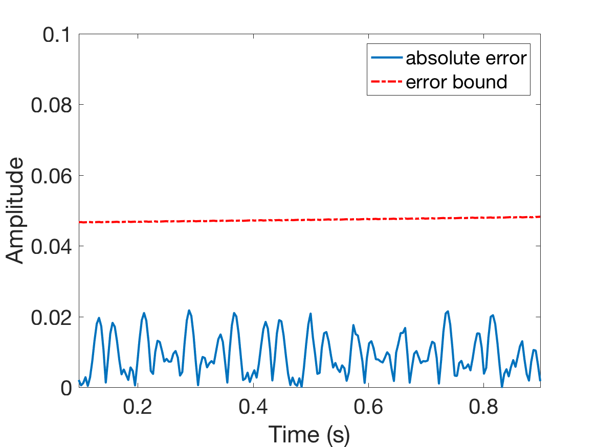
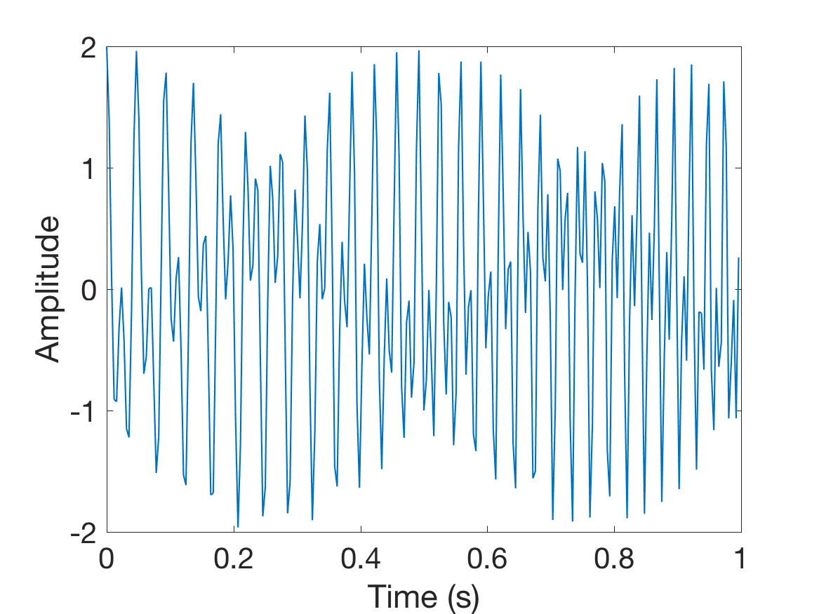
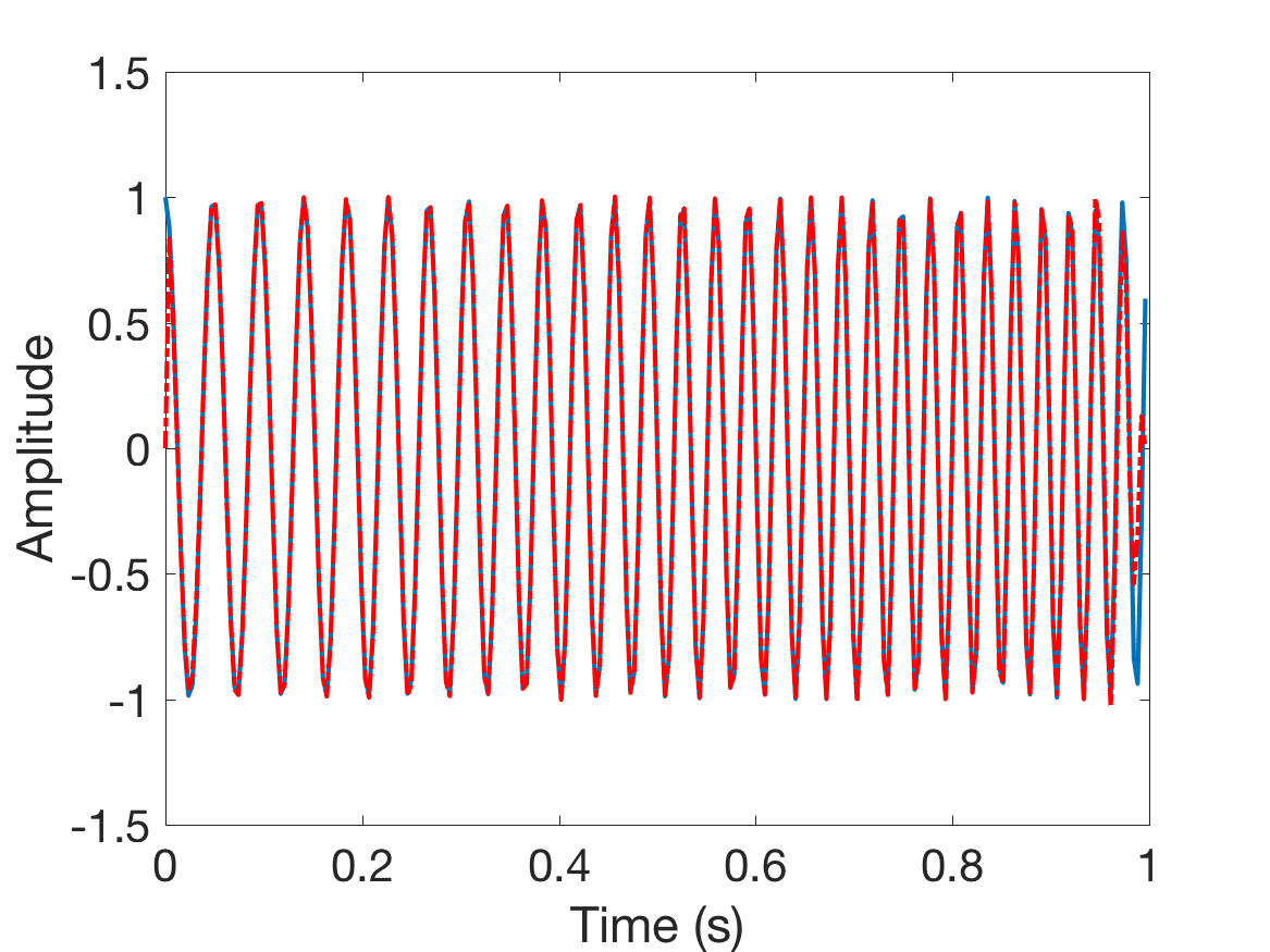
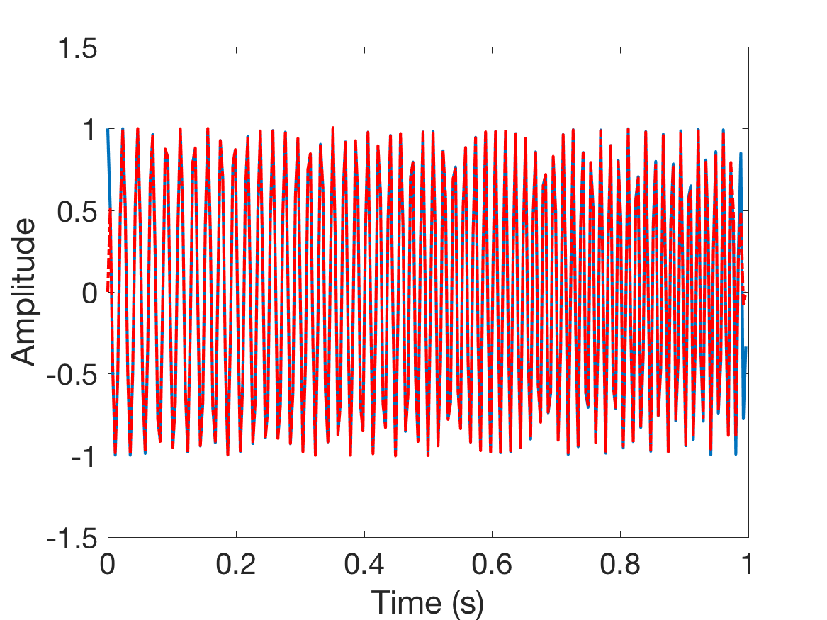
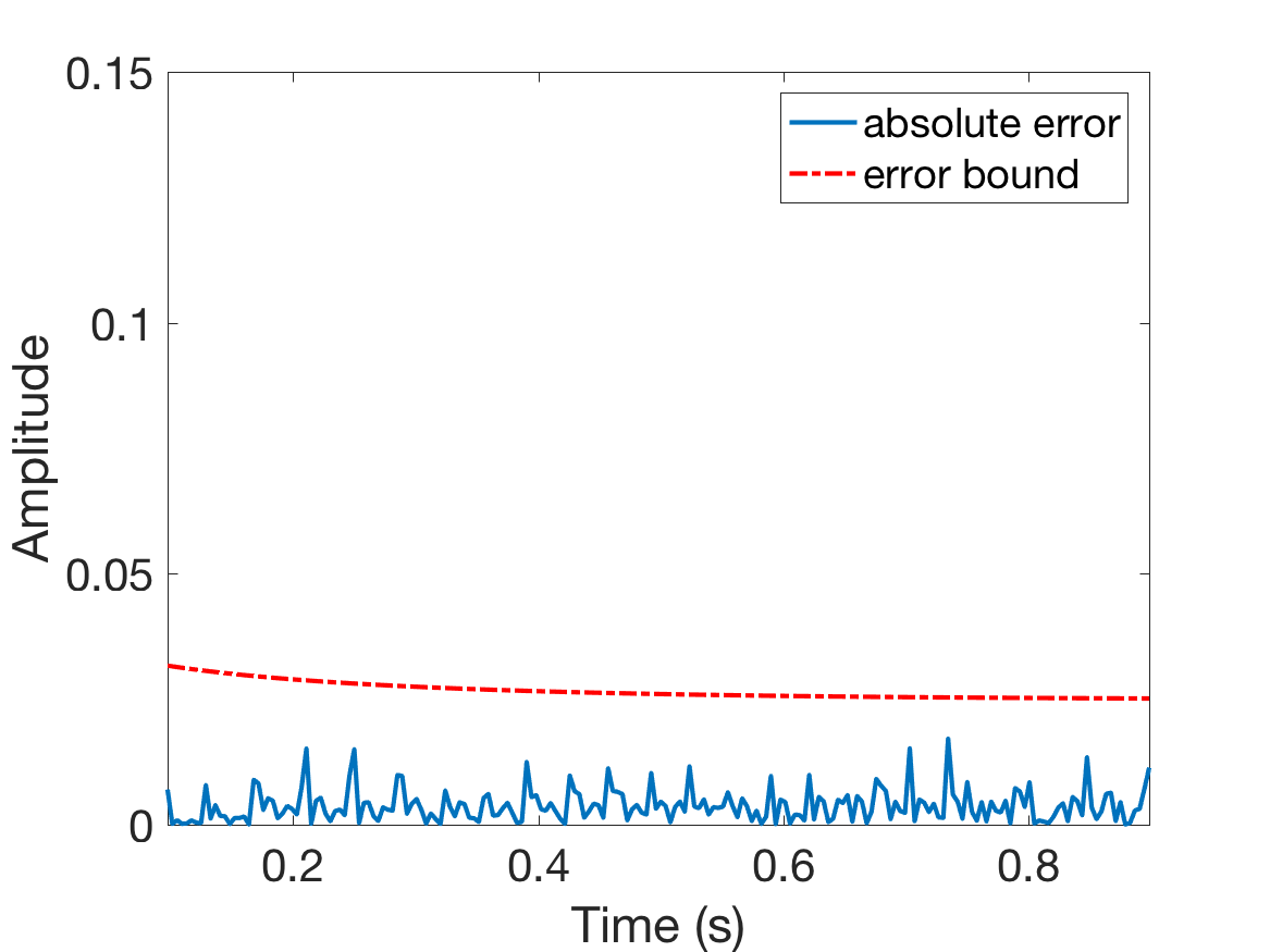
Figure 1: Example of two-component signal in (65).
Top: Waveform;
Middle-left: and recovered (red dot-dash line); Middle-right: and recovered (red dot-dash line);
Bottom-left: Absolute recovery error for and error bound ;
Bottom-right: Absolute recovery error for and error bound .
Example 1.
Let be a two-component linear frequency modulation signal given by
(65)
The number of sampling points is and the sampling rate is 256Hz.
The instantaneous frequencies of and are and , respectively.
Hence, with .
In Fig.1, we show the waveform of .
We let , and choose to be
We set and .
We show the recovered in the middle row of Fig.1.
The absolute recovery errors (the quantity on the left-hand side of (61)) for and and the error bounds and
are provided in the bottom row of Fig.1. Observe from the middle row of Fig.1 that the recovery errors are small except near boundary points and due to the boundary issue. Hence, we show the errors for in the bottom row of Fig.1.
4 Analysis of 2nd-order adaptive WSST
In this section we consider multicomponent signals of (11)
satisfying
the following conditions:
(66)
We also assume each is well approximated locally by linear chirp signals of (31)
with and small:
(67)
for some small positive numbers . More precisely, write as
Therefore, approximates well if are small. Note that
is a linear combination of linear chirps with variable .
Next we consider the approximation of when is approximated by .
With (68), we have
(72)
where
(73)
For given , we use to denote the Fourier transform of , namely,
where denotes the Fourier transform. Note that depends on also if . We drop in
for simplicity. Thus we have
(74)
Note that to distinguish the different types of the remainders for the expansion of resulted from different local approximations for ,
in this section we use “”, which means residual, to denote the remainder for the expansion of in (72). By (71), we have the following estimate for :
By (75), we know is small if are small enough. Hence, in this case determines the scale-time zone for .
More precisely, let be a given small number as the threshold.
Denote
If is even and decreasing for .
Then can be written as
(76)
where is obtained by solving In general depends on both and , and it is hard to obtain the explicit expressions for the boundaries of .
As suggested in [24], in this paper, we assume can be replaced by with
such that defined by (76) with can be written as
(77)
for some , and
(78)
In addition, we will assume the multicomponent signal is well-separated, that is there is such that
(79)
or equivalently
(80)
Next we consider the case that is the Gaussian function defined by (25) as an example to illustrate our approach. One can obtain for this (see [24]),
(81)
Thus
(82)
Therefore, in this case,
assuming (otherwise, for any ),
In the following we assume given by (11) satisfy (37) and (66), and that the adaptive CWTs
of its components with a window function
lie within scale-time zones in the sense that
(78) holds and each is given by (77).
In addition, we assume is well-separated, that is there is such that (80) holds. Let denote the set of such multicomponent signals
satisfying (67).
Next we introduce more notations to describe our main theorems on the 2nd-order adaptive WSST. For , denote
Clearly
We also denote
and denote
(89)
Recall that and denote respectively the adaptive CWTs defined by (21) with replaced by and , where are defined by
(28). Expand and as in (72), and let , , and be the corresponding residuals.
Then , , , and are given as in (73) with replaced respectively by , , , and . Thus we have the estimates for these residuals similar to (75). More precisely, we have
Next we provide Theorem 2 on the 2nd-order adaptive WSST.
The proof of Part (b) of Theorem 2 is based on the following three lemmas whose proofs are postponed to Appendix C. The residuals in these lemmas are defined as
(91)
where
with and are the errors defined by (73) with replaced by and respectively.
Suppose for some small . Then we have the following.
(a) Suppose satisfies . Then for with , there exists such that .
Suppose satisfies , , and .
Then
(96)
where
Furthermore,
(97)
where
(98)
(c) Suppose that satisfies the condition in part (a) and ,
where is defined by (60).
Then for any satisfying , we have
(99)
where
(100)
and with
(101)
and denoting the Lebesgue measure of the set :
(102)
Note that the error bound for the component recovery (99) also depends on the Lebesgue measure of the set . This makes sense since defined by (34)
takes the integral along the set
namely, does not take account of in .
Thus only in the case that is small, the integral of in
(99) can provide accurate component recovery.
Next we consider another type of 2nd-order WSST defined by (35), where the integral is taken along . To this regard, for a given , denote
(103)
Theorem 3.
Suppose with a window function
for some small . Then besides (a) in Theorem 2, the following hold:
Suppose with , we have
(104)
where
(105)
Suppose satisfies and . Then
(106)
Thus, for , we have
(107)
Suppose that satisfies the condition in part (a) of Theorem 2.
In addition, suppose the following two conditions hold: (i) , (ii) , where is given in (60).
Then for any satisfying ,
(108)
where is defined by (100), and is defined by (101).
The proofs of Theorems 2 and 3 will be provided in Appendix B.
Compared with (99), the integral of in
(108) provides more accurate component recovery. However, in this case there is a restriction on
on the set : .
The error bounds
, , in (98),
(105) and (107) for instantaneous frequency estimates are determined by and . From their definitions in (91), we know and are bounded by
, and/or , , , and/or , for (refer to (90)), and , where is defined as with replaced respectively by
Under decay conditions on and , , , , are small for , while , ,
are small as long as are small. Thus and are small.
For the component recovery error bounds in (99) and (108), are small if has certain decay. Thus under certain extra conditions, Theorem 2 and 3 can be stated in the formulation in Corollary 1.
Finally we consider another example to illustrate the recovery error bounds in
(108).
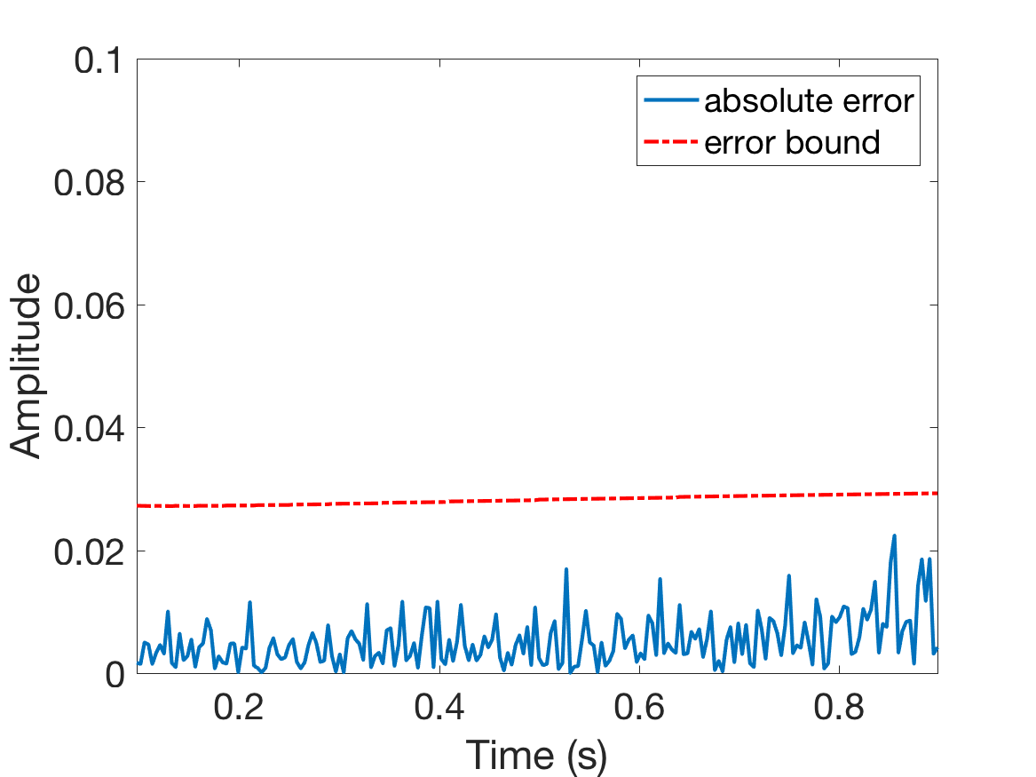
Example 2.
Let be another two-component linear frequency modulation signal given by
(109)
Again we set the number of sampling points to be and the sampling rate 256Hz.
The instantaneous frequencies of and are and , respectively. Clearly and have fast changing frequencies.
In Fig.2, we show the waveform of .
Figure 2: Example of two-component signal in (109).
Top: Waveform;
Middle-left: and recovered (red dot-dash line); Middle-right: and recovered (red dot-dash line);
Bottom-left: Absolute recovery error for and error bound ;
Bottom-right: Absolute recovery error for and error bound .
We choose , and to be defined by (87).
We set , . In addition, we use and given by (83).
We show the recovered in the middle row of Fig.2.
The absolute recovery errors for and and the error bounds and are provided in the bottom row of Fig.2. From Fig.2, we know the recovery errors are small except near boundary points and .
Proof of Theorem 1 Part (c).
Following similar discussions in [14], one can obtain that
(110)
where
Next we show that is the set defined by
Indeed, by Theorem 1 Part (b), if , then . Thus . Hence . On the other hand, suppose . Since , by Theorem 1 Part (a), for an in . If , then by Theorem 1 Part (b),
since .
This contradicts to the assumption since . Hence and . Thus we get . This , together with (110), leads to
Proof of Theorem 3 Part . By (92) in Lemma 1, we have
This shows (106). (107) follows from (106) and the assumption .
Proof of Theorem 3 Part (c). First we have the following result which can be derived as that on p.254 in [14]:
(116)
where
Let
Next we show that . By Theorem 3 Part (b1)(b2), if , then since . Thus . Hence .
On the other hand, suppose . Since , by Theorem 2 Part (a), for an in . If , then
and this contradicts to the assumption with , where we have used the fact and
by Theorem 3 Part (b1)(b2).
Hence and . Thus we know . This and (116) imply
(117)
The estimate (115), together with (117), leads to (108).
This completes the proof of Theorem 3 Part (c).
Proof of Lemma 3. (3) follows immediately
from (92) if . Thus to prove Lemma 3, it is enough to show . By the definition of in (4),
one can easily obtain that for ,
By this and direct calculations, one can get
.
So we need merely to show .
To this regard, first we notice that
This follows from and . The latter can be verified straightforward by the definition of . Thus, we have
[1] F. Auger, P. Flandrin, Y. Lin, S.McLaughlin, S. Meignen, T. Oberlin, and H.-T. Wu, “Time-frequency reassignment and synchrosqueezing: An overview,” IEEE Signal Process. Mag., vol. 30, no. 6, pp. 32–41, 2013.
[2] R. Behera, S. Meignen, and T. Oberlin, “Theoretical analysis of the 2nd-order synchrosqueezing transform,”
Appl. Comput. Harmon. Anal., vol. 45, no. 2, pp. 379–404, 2018.
[3] A.J. Berrian and N. Saito, “Adaptive synchrosqueezing based on a quilted short-time Fourier transform,” arXiv:1707.03138v5, Sep. 2017.
[4] H.Y. Cai, Q.T. Jiang, L. Li and B.W. Suter, “Analysis of adaptive short-time Fourier transform-based synchrosqueezing transform,” Analysis and Applications, 2020. https://doi.org/10.1142/S0219530520400047
[5] C.K. Chui, An Introduction to Wavelets, Academic Press, 1992.
[6] C.K. Chui and Q.T. Jiang, Applied Mathematics—Data
Compression, Spectral Methods, Fourier Analysis, Wavelets and
Applications, Amsterdam: Atlantis Press, 2013.
[7] C.K. Chui, Y.-T. Lin, and H.-T. Wu, “Real-time dynamics acquisition from irregular samples - with application to anesthesia evaluation,” Anal. Appl., vol. 14, no. 4, pp. 537–590, 2016.
[8] C.K. Chui and H.N. Mhaskar, “Signal decomposition and analysis via extraction of frequencies,” Appl. Comput. Harmon. Anal., vol. 40, no. 1, pp. 97–136, 2016.
[9] C.K. Chui and M.D. van der Walt, “Signal analysis via instantaneous frequency estimation of signal components,” Int’l J. Geomath., vol. 6, no. 1, pp. 1–42, 2015.
[10] A. Cicone. “Iterative Filtering as a direct method for the decomposition of nonstationary signals,” Numerical Algorithms, vol. 373, 112248, 2020.
[11] A. Cicone, J.F. Liu, and H.M. Zhou, “Adaptive local iterative filtering for signal decomposition and instantaneous frequency analysis,” Appl. Comput. Harmon. Anal., vol. 41, no. 2, pp. 384–411, 2016.
[12] A. Cicone and H.M. Zhou, “Numerical analysis for iterative filtering with new efficient implementations based on FFT,” preprint. Arxiv: 1802.01359.
[13] I. Daubechies, Ten Lectures on Wavelets, SIAM, CBMS-NSF Regional Conf. Series in Appl. Math, 1992.
[14] I. Daubechies, J.F. Lu, and H.-T. Wu, “Synchrosqueezed wavelet transforms:
An empirical mode decomposition-like tool,” Appl. Comput. Harmon. Anal., vol. 30, no. 2, pp. 243–261, 2011.
[15] I. Daubechies and S. Maes, “A nonlinear squeezing of the continuous wavelet transform based on auditory nerve models,” in A. Aldroubi, M. Unser Eds. Wavelets in Medicine and Biology, CRC Press, 1996, pp. 527–546.
[16] P. Flandrin, G. Rilling, and P. Goncalves, “Empirical mode decomposition as a filter bank,” IEEE Signal Proc. Letters, vol. 11, no. 2, pp. 112–114, Feb. 2004.
[17] K. He, Q. Li, and Q. Yang, “Characteristic analysis of welding crack acoustic emission signals using synchrosqueezed wavelet transform,” J. Testing and Evaluation, vol. 46, no. 6, pp. 2679–2691, 2018.
[18] C.L. Herry, M. Frasch, A. J. Seely1, and H. -T. Wu, “Heart beat classification from single-lead ECG using the synchrosqueezing transform,” Physiological Measurement, vol. 38, no. 2, 2017.
[19] N.E. Huang, Z. Shen, S.R. Long, M.L. Wu, H.H. Shih, Q. Zheng, N.C. Yen, C.C. Tung, and H.H. Liu, “The empirical mode decomposition and Hilbert spectrum for nonlinear and nonstationary time series analysis,” Proc. Roy. Soc. London A, vol. 454, no. 1971, pp. 903–995, 1998.
[20] Q.T. Jiang and B.W. Suter, “Instantaneous frequency estimation based on synchrosqueezing wavelet transform,” Signal Proc., vol. 138, no. pp. 167–181, 2017.
[21] C. Li and M. Liang, “A generalized synchrosqueezing transform for enhancing signal time-frequency representation,” Signal Proc., vol. 92, no. 9, pp. 2264–2274, 2012.
[22] C. Li and M. Liang, “Time frequency signal analysis for gearbox fault diagnosis using a generalized synchrosqueezing transform,” Mechanical Systems and Signal Proc., vol. 26, pp. 205–217, 2012.
[23] L. Li, H.Y. Cai, H.X. Han, Q.T. Jiang and H.B. Ji, “Adaptive short-time Fourier transform and synchrosqueezing transform for non-stationary signal separation,” Signal Proc.,
vol.166, January 2020, 107231. https://doi.org/10.1016/j.sigpro.2019.07.024
[24] L. Li, H.Y. Cai and Q.T. Jiang, “Adaptive synchrosqueezing transform with a time-varying parameter for non-stationary signal separation,” Appl. Comput. Harmon. Anal., in press, 2020.
https://doi.org/10.1016/j.acha.2019.06.002
[25] L. Li, H.Y. Cai, Q.T. Jiang and H.B. Ji, “An empirical signal separation algorithm based on linear time-frequency analysis,” Mechanical Systems and Signal Proc.,
vol. 121, pp. 791–809, 2019.
[26] L. Li and H. Ji, “Signal feature extraction based on improved EMD method,” Measurement, vol. 42, pp. 796–803, 2009.
[27] L. Lin, Y. Wang, and H.M. Zhou, “Iterative filtering as an alternative algorithm for empirical mode decomposition,” Adv. Adapt. Data Anal., vol. 1, no. 4, pp. 543–560, 2009.
[28] J.F. Lu and H.Z. Yang, “Phase-space sketching for crystal image analysis based on synchrosqueezed transforms,” SIAM J. Imaging Sci., vol. 11, no. 3, pp.1954–1978, 2018.
[29] S. Meignen, T. Oberlin, and S. McLaughlin, “A new algorithm for multicomponent signals analysis based on synchrosqueezing: With an application to signal sampling and denoising,” IEEE Trans. Signal Proc., vol. 60, no. 11, pp. 5787–5798, 2012.
[30] Y. Meyer, Wavelets and Operators, Volume 1, Cambridge University Press, 1993.
[31] T. Oberlin and S. Meignen, “The 2nd-order wavelet synchrosqueezing transform,” in 2017 IEEE International Conference on Acoustics, Speech and Signal Processing (ICASSP), March 2017, New Orleans, LA, USA.
[32] T. Oberlin, S. Meignen, and V. Perrier, “An alternative formulation for the empirical mode decomposition,” IEEE Trans. Signal Proc.,
vol. 60, no. 5, pp. 2236–2246, 2012.
[33] T. Oberlin, S. Meignen, and V. Perrier, “The Fourier-based synchrosqueezing
transform,” in Proc. 39th Int. Conf. Acoust., Speech,
Signal Proc. (ICASSP), 2014, pp. 315–319.
[34] T. Oberlin, S. Meignen, and V. Perrier,“Second-order synchrosqueezing transform or invertible reassignment? Towards ideal time-frequency representations,” IEEE Trans. Signal Proc.,
vol. 63, no. 5, pp. 1335–1344, 2015.
[35] D.-H. Pham and S. Meignen, “High-order synchrosqueezing transform for multicomponent signals analysis - with an application to gravitational-wave signal,” IEEE Trans. Signal Proc., vol. 65, no. 12, pp. 3168–3178, 2017.
[36] D.-H. Pham and S. Meignen,
“Second-order synchrosqueezing transform: the wavelet case and comparisons,” preprint, Sep. 2017.
HAL archives-ouvertes: hal-01586372
[37] G. Rilling and P. Flandrin, “One or two frequencies? The empirical mode decomposition answers,” IEEE Trans. Signal Proc., vol. 56, pp. 85–95, 2008.
[38] Y.-L. Sheu, L.-Y. Hsu, P.-T. Chou, and H.-T. Wu, “Entropy-based time-varying window width selection for nonlinear-type time-frequency analysis,” Int’l J. Data Sci. Anal., vol. 3, pp. 231–245, 2017.
[39] G. Thakur and H.-T. Wu, “Synchrosqueezing based recovery of instantaneous frequency from nonuniform samples,” SIAM J. Math. Anal., vol. 43, no. 5, pp. 2078–2095, 2011.
[40] M.D. van der Walt, “Empirical mode decomposition with shape-preserving spline interpolation,”Results in Applied Mathematics, in press, 2020.
[41] S.B. Wang, X.F. Chen, G.G. Cai, B.Q. Chen, X. Li, and Z.J. He, “Matching demodulation
transform and synchrosqueezing in time-frequency analysis,”
IEEE Trans. Signal Proc., vol. 62, no. 1, pp. 69–84, 2014.
[42] S.B. Wang, X.F. Chen, I.W. Selesnick, Y.J. Guo, C.W. Tong and X.W. Zhang,
“Matching synchrosqueezing transform: A useful tool for characterizing signals with fast varying instantaneous frequency and application to machine fault diagnosis,” Mechanical Systems and Signal Proc., vol. 100, pp. 242–288, 2018.
[43] Y. Wang, G.-W. Wei and S.Y. Yang , “Iterative filtering decomposition based on local spectral evolution kernel,” J. Scientific Computing, vol. 50, no. 3, pp. 629–664, 2012.
[44] H.-T. Wu, Adaptive Analysis of Complex Data Sets, Ph.D. dissertation, Princeton Univ., Princeton, NJ, 2012.
[45] H.-T. Wu, Y.-H. Chan, Y.-T. Lin, and Y.-H. Yeh, “Using synchrosqueezing transform to discover breathing dynamics from ECG signals,”Appl. Comput. Harmon. Anal., vol. 36, no. 2, pp. 354–459, 2014.
[46] H.-T. Wu, R. Talmon, and Y.L. Lo, “Assess sleep stage by modern signal processing techniques,” IEEE Trans. Biomedical Engineering, vol. 62, no. 4, 1159–1168, 2015.
[47] Z. Wu and N. E. Huang, “Ensemble empirical mode decomposition: A noise-assisted data analysis method,” Adv. Adapt. Data Anal., vol. 1, no. 1, pp. 1–41, 2009.
[48] H.Z. Yang, “Synchrosqueezed wave packet transforms and diffeomorphism based spectral analysis for 1D general mode decompositions,” Appl. Comput. Harmon. Anal., vol. 39, no.1, pp. 33–66, 2015.
[49] H.Z. Yang, “Statistical analysis of synchrosqueezed transforms,” Appl. Comput. Harmon. Anal., vol. 45, no. 3, pp. 526–550, 2018.
[50] H.Z. Yang, J.F. Lu, and L.X. Ying,
“Crystal image analysis using 2D synchrosqueezed transforms,” Multiscale Modeling Simulation, vol. 13, no. 4, pp. 1542–1572, 2015.
[51] H.Z. Yang and L.X. Ying, “Synchrosqueezed curvelet transform for two-dimensional mode decomposition,” SIAM J. Math Anal., vol 46, no. 3, pp. 2052–2083, 2014.
[52] Y. Xu, B. Liu, J. Liu, and S. Riemenschneider, “Two-dimensional empirical mode decomposition by finite elements,” Proc. Roy. Soc. London A, vol. 462, no. 2074, pp. 3081–3096, 2006.