Polarimetric SAR Image Semantic Segmentation with 3D Discrete Wavelet Transform and Markov Random Field

Abstract

Polarimetric synthetic aperture radar (PolSAR) image segmentation is currently of great importance in image processing for remote sensing applications. However, it is a challenging task due to two main reasons. Firstly, the label information is difficult to acquire due to high annotation costs. Secondly, the speckle effect embedded in the PolSAR imaging process remarkably degrades the segmentation performance. To address these two issues, we present a contextual PolSAR image semantic segmentation method in this paper. With a newly defined channel-wise consistent feature set as input, the three-dimensional discrete wavelet transform (3D-DWT) technique is employed to extract discriminative multi-scale features that are robust to speckle noise. Then Markov random field (MRF) is further applied to enforce label smoothness spatially during segmentation. By simultaneously utilizing 3D-DWT features and MRF priors for the first time, contextual information is fully integrated during the segmentation to ensure accurate and smooth segmentation. To demonstrate the effectiveness of the proposed method, we conduct extensive experiments on three real benchmark PolSAR image data sets. Experimental results indicate that the proposed method achieves promising segmentation accuracy and preferable spatial consistency using a minimal number of labeled pixels.

I Introduction

The past few decades witnessed significant progress in polarimetric synthetic aperture radar (PolSAR) theories and applications. With the flourish of airborne and spaceborne PolSAR systems, massive high-resolution PolSAR images are collected nowadays. PolSAR image semantic segmentation, the process of dividing PolSAR images into different terrain categories, has received increasing attentions in modern civil and military applications. A great variety of state-of-the-art PolSAR image segmentation approaches have been proposed in recent years [18, 14, 19, 15, 1, 3, 2, 10, 4, 5, 11, 12, 9, 34, 22, 23, 24, 26, 27, 29, 16, 20, 21, 7, 8, 13, 31, 17, 30, 32, 33, 6, 25, 28, 36, 35].

However, despite the rapid progress, there are still some challenges in PolSAR image semantic segmentation. Firstly, it is well acknowledged that high-quality annotated data is difficult to acquire, which is extremely severe in PolSAR data processing task. Annotation of the PolSAR image is not only labor-intensive and time-consuming, but also demanding specialty-oriented knowledge and skills, which leads to the scarcity of ground truth semantic information. Secondly, PolSAR images are susceptible to speckle noise caused by the coherent imaging mechanism of PolSAR systems, which dramatically degrades the quality of PolSAR images and the following segmentation performance.

A great number of methods have been proposed to address the above two issues [1, 2, 3, 10, 4, 5, 8, 7, 9, 6]. One primary strategy is using more representative features, such as wavelet analysis [1], Gabor filtering[2] and convolutional neural network (CNN) [3, 4, 5, 6] etc. Compared with the original polarimetric indicators, these extracted features incorporate local semantic information by convolutional operations over a specified region, yielding higher spatial consistency, which can effectively depress speckle noise. In addition, a group of discriminative and representative features are beneficial for the classifier to approach the decision boundary, and therefore relieves the reliance of classifiers on annotations. Another strategy dedicates to enforcing the local consistency on pixel labels. Typical approaches include the over-segmentation technique utilized in preprocessing step and graph-based optimization executed as a post-processing process. Over-segmentation technique divides the whole PolSAR image into small homogeneous patches or superpixels which are considered as an integral part in the following classifier learning and labeling process [8, 7]. Pixels in each patch share the same label during the segmentation. Graph-based optimization incorporates label smoothness priors into the segmentation task by solving a maximum a posterior (MAP) problem [2, 9, 10, 4]. With the integrated contextual consistency priors, the speckle noise in PolSAR images can be effectively depressed, producing segmentation results with higher classification accuracy and better spatial connectivity.

Both the above two strategies can effectively promote the performance of PolSAR image semantic segmentation. However, most of the existing PolSAR image segmentation methods usually consider only one of them. It is worth noting that although the prevailing deep neural networks are capable of learning discriminative and data-driven features, their performance is subject to the availability of large amounts of annotated data which require great efforts of experienced human annotators. In addition, the time consumption of deep neural networks is usually high. Therefore, to make the most advantage of contextual semantic information, and reduce the time consumption and the reliability on annotations, we propose a new PolSAR image semantic segmentation pipeline in this work. The main inspiration is to integrate multi-scale texture features and semantic smoothness priors into a principled framework. Specifically, we use the three-dimensional discrete wavelet transform (3D-DWT) to extract multi-scale PolSAR features. By incorporating the connections between features in the third dimension, the 3D-DWT features are more representative than traditional 2-dimensional (2D) texture features, yet could be extracted without complex learning process. Then, we utilize Markov Random Field (MRF) to refine the segmentation results by enforcing label smoothness and the alignment of label boundaries with image edges. It can effectively counteract speckle noise while achieving better spatial connectivity and classification accuracy. The main contributions of this work are summarized as follows:

(1) We formulate the spatial semantic features using 3D-DWT and label smoothness priors using MRF into a principled framework. To the best of our knowledge, this is the first work that simultaneously incorporates 3D-DWT and MRF into PolSAR image semantic segmentation.

(2) Different from traditional MRF models which only incorporate label smoothness priors, our defined MRF not only encourages the spatial consistency but also enforces the alignment of label boundaries with image edges. Belief propagation (BP) algorithm is employed to optimize the MRF model due to its fast convergence.

(3) To evaluate the performance of the proposed method, we conduct extensive experiments on three real benchmark PolSAR images. Experimental results show the advantages of our proposed method compared with the other eight competing PolSAR image semantic segmentation methods.

The remainder of this paper is organized as follows. We introduce the preliminaries, including the related works of PolSAR image semantic segmentation, 3D-DWT and graph model in Section II. Then, we describe the proposed method, including the raw polarimetric indicators, 3D-DWT feature extraction, SVM-MRF based supervised classification model and the model optimization in Section III. Section IV reports experimental results on three real benchmark PolSAR images. Conclusions and future works are discussed in Section V.

II Preliminaries

II-A Related works

Considering the foundations of current PolSAR image semantic segmentation methods, we broadly divide them into three categories: scattering mechanism-based methods, statistics-based methods and machine learning-based methods, which will be detailed below.

II-A1 Scattering mechanism-based methods

This category of methods conduct segmentation based on diverse polarimetric target decomposition methods, from which various terrain classes can be derived with explicit physical meanings. The most classical scattering mechanism-based method is the $H/\bar{\alpha}$ segmentation approach proposed by Cloude and Pottier [14]. In this method, eigenanalysis is firstly performed on polarimetric coherency matrix, constructing a 2-D feature plane using the extracted scattering entropy H and average scattering angle $\bar{\alpha}$. The $H/\bar{\alpha}$ plane is then divided into eight subspaces which represent diverse scattering mechanisms. Based on this subspace division, each pixel can be projected to one of the eight primary zones, determining its terrain category finally. Other commonly employed target decomposition methods include Freeman decomposition[15] and four-component decomposition[16] etc.

II-A2 Statistics-based methods

With the development of polarimetric theories, researchers discovered that polarimetric data comply with certain statistical laws. Lee et al. proposed the complex Wishart distribution for both coherency matrix and covariance matrix. Based on this hypothesis, a Wishart distance was defined to reveal the similarity of a pixel to a certain terrain clustering center[17, 18]. Lee et al. innovatively combined polarimetric distribution with target decomposition theories[19]. Specifically, an initial segmentation is firstly conducted using $H/\bar{\alpha}$ decomposition, and then the segmentation map is iteratively updated based on Wishart distance. In addition to the complex Wishart distribution, other polarimetric statistical hypotheses as $K$-distribution[20] and $\mathcal{U}$-distribution [9] were also brought forward and employed in PolSAR image semantic segmentation task [21, 10, 4].

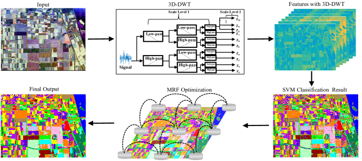
Figure 1: Illustration of our proposed method. The whole pipeline includes three steps. In step 1, based on the raw features extracted from PolSAR data, 3D-DWT is employed to generate spatial texture features. In step 2, SVM is used to generate class probabilities and a preliminary classification map. In step 3, MRF optimization is conducted to refine the classification map.

II-A3 Machine learning-based methods

Machine learning approach has dominated the PolSAR image semantic segmentation task in recent years. Bayesian classification method was firstly introduced to PolSAR image segmentation by Kong et al[22]. Pottier et al.[23] and Antropov et al.[24] applied neural network in PolSAR image semantic segmentation. Support vector machine (SVM) was extensively employed in this task [26, 25, 1, 2], producing desirable segmentation results due to its elaborate optimization architecture and good generalization ability. Most recently, the advent of deep learning techniques provided a new way for PolSAR image segmentation. Zhou et al.[3] and Bi et al. [4, 5] exploited convolutional neural network (CNN) to extract hierarchical polarimetric features. Deep belief network was applied to PolSAR image segmentation by Liu et al [27]. Zhang et al. [28] utilized stacked sparse autoencoder to learn deep spatial sparse features of PolSAR. Jiao et al. [29] designed a PolSAR image segmentation method based on deep stacking network. Chen et al. [30] proposed a novel semicoupled projective dictionary pair learning method (DPL) with stacked auto-encoder (SAE) for PolSAR image classification. The SAE is utilized to obtain hierarchical features, while SDPL is employed to reveal the intrinsic relationship between different features and perform classification. MRF technique has also been employed in PolSAR image segmentation task. Wu et al. [8] proposed a region-based PolSAR image segmentation method which combines MRF and Wishart distribution. Liu et al. [31] designed a PolSAR image segmentation method based on Wishart triplet Markov field (TMF). Masjedi et al.[2] incorporated texture features and contextual information realized by MRF technique in PolSAR image segmentation. Doulgeris et al.[9] put forward an automatic MRF segmentation algorithm based on $\mathcal{U}$-distribution for PolSAR images. In addition, these are new trends of multi-dimentional PolSAR image analyses. Xu et al. [32, 33] recently proposed novel POLSAR image analysis methods which exploit spatial and aspect dimensions jointly with polarimetric features.

Investigating the theories and performances of these PolSAR image semantic segmentation methods, we can discover that: 1) Methods falling into the first two categories are simple, fast, and physically interpretable, however, the segmentation results are coarse and imprecise, making them only suitable for preliminary analysis of PolSAR data. 2) Machine learning-based methods, especially the supervised methods, achieve better segmentation performance than the former two categories of methods. However, they rely heavily on large amounts of annotated data, even for the most popular deep learning-based methods. In addition, the deep learning-based methods usually consume a long running time. 3) By incorporating contextual information, MRF effectively improves segmentation performance and enforces label smoothness.

Inspired by the above analysis, we aim to explore more discriminative polarimetric features and fully utilize the contextual information of PolSAR data in this work. Specifically, 3D-DWT is firstly employed to extract multi-scale contextual polarimetric features. Moreover, a newly defined MRF model is further applied to refine the segmentation map, which not only enforces label smoothness, but also encourages the alignment of label boundaries with image edges.

II-B Wavelet analysis

The wavelet transform (WT) [38] is a popular mathematical tool for time-frequency analysis. Through dilating and shifting operation, sets of wavelets are generated from the original mother wavelet, which can be used to analyze different proportions of signals. Specific for image processing, the high-frequency proportion represents small-scale details, such as the edges of images, while the low-frequency proportion corresponds to the smoothing part of images.

The advent of multi-resolution analysis (MRA) [39] dramatically promoted the practical application of wavelet analysis. MRA aims at constructing a set of orthogonal wavelet bases which can infinitely approximate $L^{2}(R)$ space in the frequency domain. This provides an efficient way to analyze various proportions of signals. Owing to its outstanding localization characteristics and multi-resolution analysis ability, wavelet analysis has been extensively applied in multiple fields, including image processing, audio analysis, and theoretical physics etc[1, 2]. The commonly utilized wavelets include Haar wavelet, Daubechies wavelet, and Morlet wavelet etc.

II-C Graph Model in Image Segmentation

Graph model is one of the most important models in image processing owing to its solid mathematical foundation [40]. It provides a convenient approach to depict the local consistency between pixels in an image. For image segmentation task, an undirected graph $\mathcal{G}=<\mathcal{V},\mathcal{E}>$ can be established over the image, where image node set $\mathcal{V}$ corresponds to pixels, and undirected edge set $\mathcal{E}$ represents the neighborhood relationship, i.e., similarities, between pixels [41]. Then the labels of $\mathcal{V}$ spread through edges $\mathcal{E}$ using an optimization function, realizing segmentation of graph $\mathcal{G}$.

If positivity and Markovianity of variables on the graph are satisfied, the graph can be regarded as an MRF. Image segmentation problem, with class labels as variables, is a typical MRF solving problem. Based on the Hammersley-Clifford theorem and Bayesian theory [42], the labeling task in MRF can be transformed to solving a MAP problem.

III The proposed method

III-A Overview of the Proposed Method

In this section, we will first define some notations, and then introduce the pipeline of the proposed method. For a given PolSAR image, the raw PolSAR feature data is defined as $\mathbf{X}\in{R^{H\times{W}\times{D}}}$, where $H$ and $W$ are the height and width of the PolSAR image, and $D$ is the dimension of the selected raw polarimetric indicator as described in Section II. The labeled training samples are denoted as ${(\mathbf{x}_{i},\mathbf{y}_{i})}_{i=1}^{n}$, where $n\ll H\times{W}$, $\mathbf{y}_{i}\in\{1,\cdots K\}$. Here, $K$ is the total number of classes. The proposed method is designed to assign label $\mathbf{y}_{i}$ to each pixel $i(i\in{1,\cdots,N)}$, where $N=H\times{W}$. We further denote $\mathbf{Y}=\{\mathbf{y}_{i}\}$ in the following sections.

Taking the Flevoland area data set 1 as example, Fig. 1 illustrates the framework of the proposed method, which formulates 3D-DWT contextual feature extraction and SVM-MRF classification into a unified model. Raw polarimetric indicators are firstly extracted from the original polarimetric matrices (Section III.B). We then implement 3D-DWT feature extraction on the raw features to obtain multi-scale contextual features (Section III.C). The consequently executed SVM-MRF classification method consists of two subproblems, i.e., SVM learning-subproblem and label propagation-subproblem (Section III.D-E). We will detail all the above components in the following paragraphs.

III-B Polarimetric Raw Indicators

We first define a raw polarimetric feature set as input of our proposed method. All the features are directly drawn from the second-order $3\times 3$ complex coherency polarimetric matrix $T$, which are shown as:

$$\{\rm{SPAN}\rm,\emph{T}_{11},\emph{T}_{22},\emph{T}_{33},|\emph{T}_{12}|,|\emph{T}_{13}|,|\emph{T}_{23}|\}\\$$

In the employed 7-dimensional (7D) feature set, SPAN ($\rm{SPAN}$=$T_{11}+T_{22}+T_{33}$) denotes the total polarimetric power. The remaining six features indicate the intensities of the diagonal and upper triangle elements of complex coherency polarimetric matrix $T$. Since the 7D features are all transformed from the original scattering matrix, they represent different spectrums of polarimetric signals, yet interrelated to each other. Therefore, they can be considered as diverse information channels of the terrain targets, which makes it a natural and straightforward choice to perform 3D-DWT on the polarimetric feature cube.

III-C 3D-DWT Feature Extraction

Define $f(x)$ as a quadratic integrable function, and $\phi(x)$ as the mother wavelet function which satisfies the admissibility condition. The wavelet analysis is defined as:

$$W_{\phi f}{(a,b)}=<f(x),\phi_{a,b}(x)>=\int f(x)\frac{1}{\sqrt{a}}\phi{(\frac{x-b}{a})}dx,$$ (1)

where $\phi_{a,b}(x)$ is wavelet basis function which is obtained from mother wavelet $\phi(x)$ through dilating and shifting operation. $a$ is called scaling parameter and $b$ is called shifting parameter.

Continuous wavelet transform (CWT) is greatly suitable for data analysis due to the detailed description of signals. However, CWT is computation resource costly and information redundant due to the similarity between wavelet components, which makes it inapplicable in practical applications. To address this problem, CWT is transformed to discrete wavelet transform (DWT) through discretization on both time domain and frequency domain.

Generally, dyadic discretization is carried out on scaling parameter $a$ as 1, $a_{0}$, $a_{0}^{2}$, $a_{0}^{3}$, …, $a_{0}^{j}$. Under scale level $a_{0}^{j}$, taking $b_{0}$ as the shifting step, $b$ is discretized as 0, $a_{0}^{j}b_{0}$, $2a_{0}^{j}b_{0}$, …, $ka_{0}^{j}b_{0}$. Then the DWT is written as:

$$W_{m,n}^{\phi}(f)=<f(x),\phi_{m,n}(x)>=\int f(x)\phi_{m,n}(x)dx,$$ (2)

where $\phi_{m,n}(x)=a_{0}^{-m/2}\phi((x-n{b_{0}}{a_{0}^{m}})/{a_{0}^{m}})$, $a_{0}$ and $b_{0}$ are dyadic scale parameter and shifting parameter, respectively.

According to multi-resolution analysis (MRA), function $f(x)$ can be approximated using a linear combination of scaling function $\psi(x)$ and wavelet function $\phi(x)$ which represent low-frequency approximation and high-frequency detail respectively. A discrete signal $f[n]$ can be approximated by

$$f(n) = \frac{1}{\sqrt{M}}\sum_{k}C_{\psi}[j_{0},k]\psi_{j_{0},k}[n]$$ (3)

$$+ \frac{1}{\sqrt{M}}\sum_{j=j_{0}}^{\infty}\sum_{k}D_{\phi}[j,k]\phi_{j,k}[n],$$

where $j_{0}$ is any starting scale, $C_{\psi}[j_{0},k]$ is called scaling coefficient, and $D_{\phi}[j,k]$ is called wavelet coefficient. In DWT, their values are:

$$C_{\psi}[j_{0},k]=\frac{1}{\sqrt{M}}\sum_{n}f(n)\psi_{j_{0},k}(n),$$

$$D_{\phi}[j,k]=\frac{1}{\sqrt{M}}\sum_{n}f(n)\phi_{j,k}(n),$$ (4)

where $f[n]$, $\psi_{j_{0},k}[n]$ and $\phi_{j,k}[n]$ are discrete functions defined on $[0,M-1]$, containing totally $M$ points.

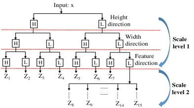
Figure 2: 3D-DWT feature extraction. The PolSAR data cube is decomposed in two scale levels. At each scale level, convolutions with all combinations of high-pass and low-pass filters in three dimensions yield eight different PolSAR data cubes. Then, the PolSAR data cube filtered by the low-pass filters in three dimensions is further decomposed in the next scale level.

In this work, we apply the 3D-DWT technique to polarimetric data cube, which encodes the contextual information to different scales. It is noteworthy that 3D-DWT can be achieved by applying 1D-DWTs to each of the three dimension. For this application, MRA decomposes the original signal into low-frequency part and high-frequency part, and then continually decomposes low-frequency part while keeping the high-frequency part unchangeable. In practice, scaling and wavelet functions are achieved using a filter bank $[L,H]$, where $L$ are low-pass filters with coefficients $C_{\psi}[j,k]$ and $H$ are high-pass filters with coefficients $D_{\phi}[j,k]$. The Haar wavelet is employed in this work, where $C_{\psi}[j,k]=(1/\sqrt{2},1/\sqrt{2})$, and $D_{\phi}[j,k]=(-1/\sqrt{2},1/\sqrt{2})$. The decomposition structure as shown in Fig.2 is employed in this work. After the 3D-DWT decomposition, 15 sub-cubes ${Z}_{1},{Z}_{2},...,{Z}_{15}$ are generated. It should be noted that the down-sampling step is left out in the process, and thus each sub-cube has the same size with the original polarimetric data cube. For pixel $(i,j)$, the 3D-DWT wavelet coefficients can be concatenated to below feature vector form.

$${z}(i,j)=({Z}_{1}(i,j,\cdot),{Z}_{2}(i,j,\cdot),\cdots,{Z}_{15}(i,j,\cdot)),$$ (5)

To further enforce spatial consistency, a $3\times 3$ square mean filter is applied to the absolute values of 3D-DWT wavelet coefficients following:

$$\bar{Z}_{k}(i,j)=\frac{1}{9}\sum_{m=i-1}^{i+1}\sum_{n=j-1}^{j+1}|{Z}_{k}(m,n,\cdot)|,k=1,2,\cdots,15,$$ (6)

We denote ${\mathbf{Z}}\in{R^{H\times{W}\times{15D}}}$ as the final concatenated feature vector in the following sections. With the 7D raw feature set (described in Section III.B) as input, the 3D-DWT feature extractor outputs 105-dimensional texture features, acting as input for the SVM classifier.

III-D SVM-MRF Classification Model

Given the extracted 3D-DWT features as input, we next introduce our proposed SVM-MRF PolSAR image semantic segmentation model. It aims to estimate class label $\mathbf{Y}$ with observation $\mathbf{Z}$ (we use the 3D-DWT features $\mathbf{Z}$ instead of the original raw features $\mathbf{X}$). To serve this propose, we define an energy function given by:

$$E=E_{d}+E_{s},$$ (7)

where $E_{d}$ indicates the SVM data loss term, and $E_{s}$ denotes the label smoothness term. The dense class labels $\mathbf{Y}$ can be predicted by minimizing this energy function,

III-D1 SVM data loss term

This term is designed to predict class labels based on the contextual 3D-DWT features, which follows the multi-class probabilistic SVM [46] as

$$E_{d}=-\sum_{i=1}^{N}log{P(\mathbf{y}_{i}|\mathbf{z}_{i})},$$ (8)

where $P(\mathbf{y}_{i}|\mathbf{z}_{i})$ denotes the probabilities of pixel $i$ belonging to class $\mathbf{y}_{i}$ with feature $\mathbf{z}_{i}$. Minimizing this term encourages that the class label with higher output probability will be preferred. The larger the probability of a pixel belonging to a certain class, the more probable that the pixel is assigned with the corresponding label.

III-D2 Label smoothness term

The label smoothness term is defined to enforce the smoothness of estimated class label map and alignment of class label boundaries with image edges, which is defined as

$$E_{s}=\alpha_{s}\sum_{i=1}^{N}\sum_{j\in\mathcal{N}(i)}\mathcal{S}_{ij},$$ (9)

where $\alpha_{s}$ is the label smoothness factor. $\mathcal{N}(i)$ is the neighboring pixel set of pixel $i$. $\mathcal{S}_{ij}$ is defined as

$$\mathcal{S}_{ij}=|\mathbf{y}_{i}-\mathbf{y}_{j}|\exp(-\frac{\|\mathbf{v}_{i}-\mathbf{v}_{j}\|_{2}^{2}}{2\sigma}),$$ (10)

where $\mathbf{v}_{i}$ is a feature vector located at pixel $i$, which should be chosen as the features whose values significantly change across edges in image. We take $\mathbf{v}_{i}$ as the Pauli matrix components in this work. $\sigma$ indicates the mean squared distance between features of two adjacent pixels $i$ and $j$. The label smoothness loss function encourages the label boundaries to align with strong image edges. For pixels $i$ and $j$ within flat regions, $\exp(-\frac{\|\mathbf{v}_{i}-\mathbf{v}_{j}\|_{2}^{2}}{2\sigma})$ in Eq. (10) is large, then minimizing $\mathcal{S}_{ij}$ will intensify the chance that labels $\mathbf{y}_{i}$ and $\mathbf{y}_{j}$ take same class label. However, for neighboring pixels spanning strong edges, $\exp(-\frac{\|\mathbf{v}_{i}-\mathbf{v}_{j}\|_{2}^{2}}{2\sigma})$ is smaller (or even near to zero), thus the inconsistency between the class labels of neighboring pixels $i$ and $j$ is allowable during optimization.

Summarized from the above formulations, the final integrated energy function can be written as

$$E=-\sum_{i=1}^{N}log{P(\mathbf{y}_{i}|\mathbf{z}_{i})}+\alpha_{s}\sum_{i=1}^{N}\sum_{j\in\mathcal{N}(i)}\mathcal{S}_{ij},$$ (11)

III-E Optimization

Label $\mathbf{Y}$ can be solved by minimizing the energy function defined in Eq. (11). We decompose this optimization problem into two subproblems, i.e. SVM learning-subproblem and Label propagation-subproblem.

III-E1 SVM learning-subproblem

For this subproblem, a multi-class probabilistic SVM classifier is firstly trained using a preselected training set based on 3D-DWT features. Next, the learned classifier is employed to predict pixel-wise class probabilities of the whole data set, providing input for the label propagation-subproblem.

III-E2 Label propagation-subproblem

Based on the trained classifier in SVM learning-subproblem, this subproblem focuses on updating label $\mathbf{Y}$ while incorporating label smoothness priors. This label assignment problem is a combinatorial optimization problem, which can be regarded as a standard MRF model[10]. The labels $\mathbf{Y}$ over the graph constitute an MRF, and Eq. (11) is the energy function on it. The two terms of the energy function enforce label constraints from the agreement between SVM predictions and target class labels, and class label smoothness, respectively. Minimizing these two terms enforces that the predicted class labels should be smooth and consistent with the SVM predictions.

Labeling problem in an MRF is a NP-hard problem. However, optimal solution can be approximately achieved using optimization algorithms [43, 44]. Belief propagation (BP) algorithm [44] iteratively optimizes MRF using an “up-down-left-right” message passing schedule in a linear time complexity, which makes the model converge very quickly. Therefore, BP algorithm is employed to optimize our defined MRF model in this work.

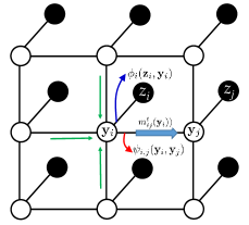
Figure 3: Message passing scheme in MRF model using BP algorithm.

Figure 3 illustrates the message passing policy of BP optimization algorithm. Each node $i$ in the MRF model corresponds to one pixel in the given PolSAR image, which can be considered as a random value. Label $\mathbf{y}_{i}$ is linked to its 3D-DWT contextual feature data $\mathbf{z}_{i}$. Let $\phi_{i}(\mathbf{z}_{i},\mathbf{y}_{i})$ represent the likelihood potential of label $\mathbf{y}_{i}$ given feature data $\mathbf{z}_{i}$, taking the form of the multi-class probabilistic SVM loss term $-\log P(\mathbf{y}_{i}=j|\mathbf{z}_{i})$ [See Eq. (8)], $\psi_{i,j}(\mathbf{y}_{i},\mathbf{y}_{j})$ stand for the label smoothness potential that encourages label contextual consistency between neighboring pixels $i$ and $j$ with form $\alpha_{s}\mathcal{S}_{ij}$ [See Eq. (9-10)]. Then at iteration $t$, the message sent from node $i$ to its neighboring node $j\in\mathcal{N}(i)$ is given by

$$\begin{split}\small m_{ij}^{t}(\mathbf{y}_{j})\leftarrow\mathop{\max}\limits_{\mathbf{y}_{i}}(\mathop{\sum}\limits_{k\in\mathcal{N}(i)\backslash j}m_{ki}^{t-1}(\mathbf{y}_{i})-\phi_{i}(\mathbf{z}_{i},\mathbf{y}_{i})-\psi_{i,j}(\mathbf{y}_{i},\mathbf{y}_{j}))\end{split}$$ (12)

With all messages initialized as 0, messages of each node are iteratively updated and propagated to its neighboring nodes until convergence. Finally, label $\mathbf{y}_{i}$ is obtained by estimating the maximum belief for node $i$, which is given by

$$\begin{split}\mathbf{y}_{i}=\mathop{\arg\max}\limits_{\mathbf{y}_{i}\in\{1,...,K\}}(\mathop{\sum}\limits_{k\in\mathcal{N}(i)}m_{ki}^{t}(\mathbf{y}_{i})-\phi_{i}(\mathbf{z}_{i},\mathbf{y}_{i}))\end{split}$$ (13)

The open source code package MRF minimization is employed to implement the BP algorithm.

III-F Summary of the Algorithm

Algorithm 1 illustrates the pipeline of the proposed method. We first extract raw features from the PolSAR data (Section III.B). Then, contextual features are extracted using the 3D-DWT technique (Section III.C). Finally, we predict class labels by optimizing our designed SVM-MRF based supervised learning model (Section III.D-E).

Algorithm 1 PolSAR Image Semantic Segmentation Using 3D Discrete Wavelet Transform and Markov Random Field

Input: Pixel-wise coherence matrix $T$, ground truth class labels, pairwise smoothness parameter $\alpha_{s}$
  Output: Pixel-wise class labels $\mathbf{Y}$

1:Extract raw features $\mathbf{X}\in{R^{H\times{W}\times{D}}}$

2:Convert $\mathbf{X}$ to ${\mathbf{Z}}\in{R^{H\times{W}\times{15D}}}$ using 3D-DWT feature extraction technique

3:Randomly select a proportion of pixels with ground truth class labels as training samples and train a multi-class SVM classifier

4:Estimate class probabilities of pixels using the trained SVM classifier

5:Predict the class labels $\mathbf{Y}$ by solving an MRF model with BP optimization algorithm

6:$\bf end$

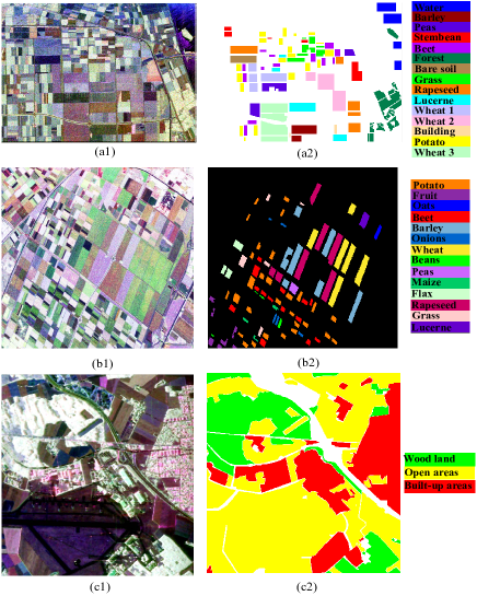
Figure 4: Experimental images. (a1) PauliRGB image of Flevoland area data set 1. (a2) Ground truth class labels and color codes of Flevoland area data set 1. (b1) PauliRGB image of Flevoland area data set 2. (b2) Ground truth class labels and color codes of Flevoland area data set 2. (c1) PauliRGB image of Oberpfaffenhofen area data set. (c2) Ground truth class labels and color codes of Oberpfaffenhofen area data set.

IV Experiments

IV-A Experimental Data and Settings

In this section, experiments on three real PolSAR data sets are conducted to validate the performance of the proposed method. Figure 4 displays the experimental images employed for evaluation. The first image was acquired by NASA/JPL AIRSAR on August 16, 1989. It is an L-band PolSAR image with size 750$\times$1024. We denote this data set as Flevoland area data set 1 in following sections. Figure 4(a1) presents the PauliRGB image of Flevoland area data set 1, and Fig. 4(a2) shows the ground truth class labels and color codes. There are 15 classes in total, including water, barley, peas, stembean, beet, forest, bare soil, grass, rapeseed, lucerne, wheat 1, wheat 2, building, potato, and wheat 3.

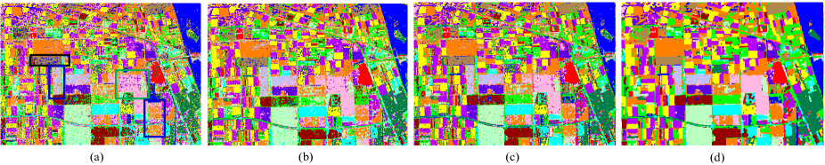
Figure 5: Ablation study of our proposed method. (a) SVMNoDWT. (b) SVM2D. (c) SVM3D. (d) SVM3D-BPMRF

TABLE I: Ablation study of our proposed method

Method	Water	Barley	Peas	Stembean	Beet	Forest	Bare soil	Grass
SVMNoDWT	96.12	90.66	88.02	80.51	73.49	83.53	74.46	45.27
SVM2D	94.37	95.23	92.57	95.09	87.15	90.83	92.46	59.07
SVM3D	97.23	95.88	92.50	95.53	94.76	93.75	96.18	67.04
SVM3D-BPMRF	98.42	97.66	97.38	98.20	99.64	98.80	99.75	83.22
Method	RapeSeed	Lucerne	Wheat 1	Wheat 2	Building	Potato	Wheat 3	Overall CA
SVMNoDWT	72.86	76.67	64.95	82.25	45.85	81.57	88.30	79.98
SVM2D	79.60	90.19	83.74	86.26	85.58	89.89	91.36	87.66
SVM3D	86.37	90.20	79.23	87.97	94.56	90.90	93.21	90.57
SVM3D-BPMRF	95.53	95.88	89.70	96.86	99.32	97.83	98.87	96.72

The second data set is another L-band image collected by AIRSAR over Flevoland area in 1991. The size of this image is 1020$\times$1024. This data set is denoted as Flevoland area data set 2 in Section IV. Figure 4(b1) displays the PauliRGB image of Flevoland area data set 2. The ground truth class labels and color codes are presented in Fig. 4(b2). Flevoland area data set 2 includes 14 classes, which are potato, fruit, oats, beet, barley, onions, wheat, beans, peas, maize, flax, rapeseed, grass, and lucerne, respectively.

Figure 4(c1) shows the PauliRGB image of the third experimental data set. It is an L-band image obtained by E-SAR, German Aerospace Center, over Oberpfaffenhofen area in Germany. The size of this image is 1300$\times$1200. The ground truth class labels and color codes are given in Fig. 4(c2). There are three labeled classes in the image: built-up areas, wood land, and open areas. The void areas are unlabeled class, which are not taken into consideration during the experiments.

In the experiments, we first conduct ablation study in Section III.B, justifying the effectiveness of the two key and novel components of the proposed method: 3D-DWT contextual features and MRF optimization. Then parameter analysis will be presented in Section III.C. Finally, in Section III.D, we demonstrate the effectiveness of the proposed method by comparison with the other eight methods listed as below.

(1) KNN method [7] which employs a Euclidean distance defined on the basis of three polarimetric PauliRGB channels.

(2) SupWishart method [19] which is supervised method based on Wishart statistical hypothesis of PolSAR data.

(3) SupWishart-PMRF method which combines supervised Wishart semantic segmentation with Potts MRF model.

(4) MLRsubMLL method [47] which combines subspace multinomial logistic regression and MRF. Graph cut method is employed to solve the MRF in this method.

(5) GGW-BPMRF method. The original paper [2] employs GLCM, Gabor and wavelet transforms of PauliRGB data as texture features, and SVM with Potts MRF model as classifier. To fairly evaluate the performance of different features, we change the Potts MRF model to BP MRF model instead.

(6) SVM3D-GCMRF method [48] which exploits 3D-DWT texture features as input feature of SVM classifier and feature similarity model for MRF optimization. Graph cut method is utilized to solve the MRF model.

(7) CNN method [3] which applies deep neural network in PolSAR image semantic segmentation.

(8) CNN-BPMRF method which integrates CNN with BP MRF into a unified framework.

We conducted quantitative comparisons on the three experimental data sets, wherein the classification accuracies and time consumptions are reported and analyzed. For convenience, we define the classification accuracy (CA) of a class as the ratio of the number of pixels correctly classified for the class to the total number of pixels in this class. The Overall CA is defined as the ratio of the number of correctly classified pixels in the whole image to the total number of pixels in the image. For all the experiments, we randomly select 1$\%$ pixels with ground truth class labels as training samples. For all SVM-based methods, in order to determine the SVM parameters, we randomly select 200 training samples from the training set to perform cross-validation. It should be noted that the cross-validation time consumption is included in the time cost analysis in Section IV. All experiments are implemented on a laptop with 2.6GHz CPU and 16GB memory.

IV-B Ablation Study

To evaluate the effectiveness of the two key components of the proposed method: 3D-DWT contextual features and MRF optimization, we conduct four groups of experiments:

(1) Using raw polarimetric features and SVM classification, without 3D-DWT contextual features and MRF optimization (Denoted as SVMNoDWT).

(2) Using 2D-DWT texture features, i.e., conducting DWT only on width and height dimensions but not on feature dimension, and SVM classification, without MRF optimization (Denoted as SVM2D).

(3) Using 3D-DWT features and SVM classification, without MRF optimization (Denoted as SVM3D).

(4) Using 3D-DWT features and SVM classification with MRF optimization (Denoted as SVM3D-BPMRF).

Taking Flevoland area data set 1 for example, Fig. 5 illustrates the semantic segmentation results under the above four comparison scenarios. Figure 5(a) shows the semantic segmentation result of SVMNoDWT, where a great deal of misclassified pixels can be observed. In the region marked by black rectangle, an appreciable part of bare soil pixels are misclassified as water class. In addition, we can find distinct class confusions between rapeseed and wheat 1 [highlighted by blue rectangles], and wheat 2 and beet [highlighted by green rectangle]. Except for the above class confusions, the whole class label map exhibits a speckle-like appearance. The reason accounting for these phenomena is that the representative ability of the raw features is weak, and the speckle noise is not effectively depressed without encoding the contextual information. Figure 5(b) displays the semantic segmentation result based on 2D-DWT features. We can discover from this figure that the speckle noise is greatly mitigated compared with Fig. 5(a). The semantic segmentation result using 3D-DWT contextual features is presented in Fig. 5(c). Compared with the class label map in Fig. 5(b), less isolated pixels and better spatial consistency can be observed in this figure, which exactly illustrates the stronger feature discrimination and contextual representation of 3D-DWT than 2D-DWT. The segmentation result of our proposed method is depicted in Fig. 5(d). It is noteworthy that the segmentation result after performing MRF optimization is in better conformity with the ground truth class labels, and exhibits less intra-class variability [37] and clearer label boundaries, which demonstrates that MRF optimization can effectively counteract the speckle noise and promote the contextual consistency.

Tables I lists the numerical results of the four comparison scenarios. We can conclude from the table that our proposed method outperforms SVMNoDWT, SVM2D, and SVM3D by 16.74%, 9.06% and 6.15% respectively, which justifies the effectiveness of feature extraction using 3D-DWT and the label smoothness enforcement of MRF. It is noticeable the Overall CA value using 3D-DWT is 2.91% higher than 2D-DWT, which validates the effectiveness of the wavelet transforms on the third dimension.

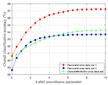
Figure 6: The influence of $\alpha_{s}$ on classification accuracy.

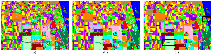
Figure 7: Semantic segmentation results for Flevoland area data with different $\alpha_{s}$. (a) $\alpha_{s}$=1 (b) $\alpha_{s}$=5 (b) $\alpha_{s}$=10.

IV-C Parameter Analysis

For the proposed method, parameter $\alpha_{s}$ which determines the tightness of label smoothness constraint significantly influences the final segmentation result. Larger $\alpha_{s}$ indicates that label smoothness term plays a more important role during the optimization, therefore tends to generate smoother semantic segmentation result. However, too large $\alpha_{s}$ will lead to loss of details. Therefore, we next analyze the impact of parameter $\alpha_{s}$, to reach a compromise between the classification accuracy and detail preservation.

Figure 6 shows the influence of parameter $\alpha_{s}$ on the Overall CA value, where $\alpha_{s}$ takes value from 0 to 10 with step size 0.5. $\alpha_{s}$$=$$0$ corresponds to the scenario without MRF optimization. It can be observed obviously from Fig. 6 that the classification accuracy increases significantly with the increment of $\alpha_{s}$ when $\alpha_{s}$ is less than 3. When $\alpha_{s}$ grows larger than 3, the increase tendency of Overall CA value slows down and roughly converges at $\alpha_{s}$$=$$5$. When $\alpha_{s}\textgreater 5$, the $\alpha_{s}$ increase brings marginal improvement on classification accuracy.

To intuitively illustrate the influence of parameter $\alpha_{s}$, taking Flevoland area data set 1 for example, we show the semantic segmentation results with $\alpha_{s}$ taking three typical values 1, 5 and 10 in Fig. 7. We can observe from Fig. 7(a) that when $\alpha_{s}$ takes the value 1, although the whole class label map is smoother than the case without MRF optimization as shown in Fig. 5(c), some speckle-like and isolated pixels still scatter in the image. Moreover, the label boundaries are not clear and straight. Figure 7(b) exhibits the semantic segmentation result with $\alpha_{s}=5$. We can discover from the figure that the speckle noise is better depressed than the result shown in Fig. 7(a), and the label boundaries are well aligned with the image edges. However, when $\alpha_{s}$ increases to value 10, although the whole image shows favorable spatial connectivity, many terrain details fade out or even disappear in the segmentation map, especially the thin and small regions. For example, the bridge in the right middle part and the road in the middle bottom part of the image [marked by black rectangles] get broken after strong smoothing. Therefore, to make a balance between the spatial connectivity and detail preservation, $\alpha_{s}$ takes the value 5 in the following experiments.

Figure 8: Semantic segmentation results of different methods on Flevoland area data set 1. (a) KNN. (b) SupWishart. (c) SupWishart-PMRF. (d) MLRsubMLL. (e) GGW-BPMRF. (f) CNN. (g) CNN-BPMRF. (h) SVM3D-GCMRF. (i) SVM3D-BPMRF.

TABLE II: CAs (%) of Flevoland area data set 1 with different methods

Method	Water	Barley	Peas	Stembean	Beet	Forest	Bare soil	Grass
KNN [7]	18.84	88.73	62.00	25.24	70.40	41.25	81.31	38.00
SupWishart [19]	52.61	45.77	88.33	83.01	74.98	86.42	59.29	65.09
SupWishartMRF	54.84	50.70	95.69	92.41	76.95	92.39	56.43	71.55
MLRsubMLL [47]	91.94	81.54	0.02	84.79	80.50	96.25	98.10	0.00
GGW-BPMRF	92.89	92.35	88.71	78.49	90.22	96.80	62.93	56.15
CNN [3]	95.38	92.48	96.19	97.02	96.11	97.95	79.62	77.50
CNN-BPMRF	97.42	96.17	98.28	97.78	98.60	98.65	91.64	83.51
SVM3D-GCMRF [48]	96.37	97.35	95.88	96.88	95.76	97.66	100.00	82.01
Our Method	98.42	97.66	97.38	98.20	99.64	98.80	99.75	83.22
Time Cost	RapeSeed	Lucerne	Wheat 1	Wheat 2	Building	Potato	Wheat 3	Overall CA
5.8 s	35.98	46.03	46.97	56.20	65.71	49.01	65.79	50.84
10.2 s	46.96	86.77	14.71	92.38	84.08	68.67	83.89	70.00
19.2 s	59.37	84.92	13.15	97.25	80.95	65.16	87.16	73.49
6 h 28 m 21.8 s	90.87	91.93	38.42	64.08	86.39	91.09	79.47	73.91
4 m 10.9 s	74.57	69.83	47.36	92.61	60.68	75.84	95.53	82.48
35 m 26.7 s	76.16	93.57	78.53	87.46	79.86	90.26	94.57	90.18
37 m 15.1 s	81.06	94.62	88.47	92.11	84.49	94.10	97.22	93.83
6 h 30 m 52.3 s	91.03	94.66	91.61	96.23	77.55	94.70	97.49	95.04
5 m 6.0 s	95.53	95.88	89.70	96.86	99.32	97.83	98.87	96.72

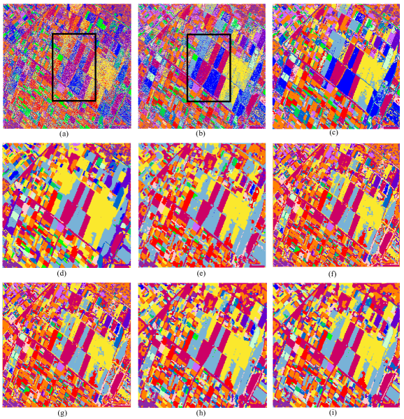
Figure 9: Semantic segmentation results of different methods on Flevoland area data set 2. (a) KNN. (b) SupWishart. (c) SupWishart-PMRF. (d) MLRsubMLL. (e) GGW-BPMRF. (f) CNN. (g) CNN-BPMRF. (h) SVM3D-GCMRF. (i) SVM3D-BPMRF.

TABLE III: CAs (%) of Flevoland area data set 2 with different methods

Method	Potato	Fruit	Oats	Beet	Barley	Onions	Wheat	Overall CA
KNN [7]	67.92	80.97	81.64	39.93	30.99	18.54	53.68	48.89
SupWishart [19]	87.24	26.33	88.52	67.93	32.39	17.18	77.85	65.78
SupWishartMRF	98.46	13.37	94.98	83.99	27.32	11.92	89.89	73.06
MLRsubMLL [47]	83.15	98.24	99.71	51.07	74.79	32.08	79.95	79.58
GGW-BPMRF	91.66	92.76	81.64	82.33	95.73	4.51	93.13	86.83
CNN [3]	90.18	93.82	68.36	72.37	83.09	32.86	88.49	86.16
CNN-BPMRF	92.81	96.37	83.00	76.10	87.50	33.05	93.44	89.75
SVM3D-GCMRF [48]	95.54	99.90	79.34	79.01	97.53	55.49	98.20	93.01
Our Method	95.01	99.91	79.25	78.48	98.44	57.79	98.77	93.43
Method	Beans	Peas	Maize	Flax	Rapeseed	Grass	Lucerne	Time Cost
KNN [7]	60.63	78.38	48.60	32.95	45.88	31.83	58.27	7.3 s
SupWishart [19]	38.17	89.54	60.85	85.98	74.59	38.18	74.09	13.1 s
SupWishartMRF	32.16	100.00	57.75	94.56	85.67	46.91	86.65	25.9 s
MLRsubMLL [47]	79.92	98.70	45.99	91.24	92.07	56.98	88.50	12 h 2 m 52.2 s
GGW-BPMRF	31.15	99.81	82.87	18.09	94.33	76.64	46.54	5 m 11.5 s
CNN [3]	53.97	98.47	61.09	90.17	96.55	66.06	84.69	41 m 8.4 s
CNN-BPMRF	54.90	99.21	82.17	94.19	97.92	71.00	88.96	43 m 17.6 s
SVM3D-GCMRF [48]	62.57	99.68	77.36	91.26	93.53	81.66	92.04	12 h 9 m 38.2 s
Our Method	62.88	100.00	72.84	92.92	94.09	82.24	95.67	7 m 22.9 s

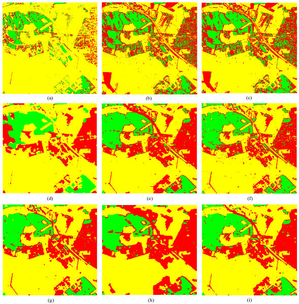
Figure 10: Semantic segmentation results for Oberpfaffenhofen area data set for different methods. (a) KNN. (b) SupWishart. (c) SupWishart-PMRF. (d) MLRsubMLL. (e) GGW-BPMRF. (f) CNN. (g) CNN-BPMRF. (h) SVM3D-GCMRF. (i) SVM3D-BPMRF.

TABLE IV: CAs (%) of Oberpfaffenhofen area data set with different methods

Method	Built-up areas	Wood land	Open areas	Overall CA	Time Cost
KNN [7]	57.83	23.55	99.75	72.95	1 m 25.0 s
SupWishart [19]	66.60	56.28	90.66	77.55	10.9 s
SupWishart-PMRF	70.27	55.72	90.04	77.79	33.4 s
MLRsubMLL [47]	74.52	72.28	99.68	88.07	27 h 5 m 51.2 s
GGW-BPMRF	89.25	87.38	97.26	93.28	12 m 25.3 s
CNN [3]	89.26	78.95	97.23	91.21	54 m 32.6 s
CNN-BPMRF	90.91	84.43	98.02	93.51	56 m 18.0 s
SVM3D-GCMRF [48]	80.11	92.09	93.89	90.73	27 h 18 m 45.7 s
Our method	90.40	86.68	97.77	93.62	15 m 31.9 s

IV-D Results and Comparisons

IV-D1 Flevoland Area Data set 1

The class label maps of Flevoland area data using the nine compared methods are presented in Fig. 8, and the CA values and time consumptions are reported in Table II.

Figure 8(a)-(b) illustrate the class label maps using KNN and SupWishart methods respectively. We can find a great number of miscellaneous labels in these two figures [marked by the black and blue rectangles in Fig. 8(a)-(b)]. This is because the KNN and Wishart distances are not discriminative enough to distinguish the confused classes with similar scattering mechanisms. SupWishart-PMRF method integrates Potts MRF priors with SupWishart method, achieving better spatial connectivity. However, the confusion between water and bare soil, rapeseed and wheat 1 classes can still be noticeably observed [marked by the black and blue rectangles in Fig. 8(c)]. Figure 8(d) presents the class label map of MLRsubMLL method. We can find obvious ambiguities between rapeseed and wheat 3 classes, and rapeseed and wheat 1 classes [marked by the blue rectangle in Fig. 7(d)]. In addition, MLRsubMLL method fails to discriminate grass class [highlighted by black rectangle in Fig. 7(d)]. The numerical results in Table II show that the Overall CA values of KNN, SupWishart, SupWishart-PMRF, and MLRsubMLL lag behind our proposed method by 45.88%, 26.72%, 23.23% and 22.81% respectively.

To better validate the effectiveness of our proposed method, we compare it with four state-of-the-art methods, i.e., GGW-BPMRF, SVM3D-GCMRF, CNN and CNN-BPMRF methods. Investigating Fig. 8(e)-(i) and Table II, we can conclude:

(1) 3D-DWT features are more representative than combinations of 2D texture features. Using the same BP MRF model, the superiority of the Overall CA value of our proposed method over GGW-BPMRF is owing to the stronger ability of 3D-DWT features in distinguishing diverse terrains.

(2) CNN fails to differentiate a number of classes with similar scattering mechanisms [marked by black and blue rectangles in Fig. 8(f)]. This is because only 1,677 training samples (1% pixels with ground truth class labels) are available in this experimental set, which results in insufficient tuning of the CNN filters due to the deep architecture of the network. The Overall CA values of CNN and CNN-BPMRF methods fall behind our proposed method by 6.54% and 2.89% respectively. Besides, our proposed method consumes much less time (5 minutes 6.0 seconds) than CNN (35 minutes 26.7 seconds) and CNN-BPMRF (37 minutes 15.1 seconds).

(3) With the same 3D-DWT features, our proposed method marginally outperforms SVM3D-GCMRF method by 1.68%. However, SVM3D-GCMRF method consumes 6 hours 30 minutes 52.3 seconds on the model convergence, while our proposed method only costs 5 minutes 6.0 seconds. The distinct lower time consumption makes our proposed method more practical in real applications.

The above conclusions gracefully demonstrate the strong discriminative ability of 3D-DWT features under low annotation scenario, and the favorable label smoothness enforcement of MRF optimization with low time consumption.

IV-D2 Flevoland Area Data set 2

Figure 9 illustrates the class label maps of the nine compared methods on Flevoland area data set 2. The numerical results of their CA values and time consumptions are reported in Table III. Observing Fig. 9(a)-(i) and Table III, we highlight below main observations:

(1) Without utilizing texture features or MRF optimization, the speckle noise in Fig.8 (a)-(b) greatly degrades the segmentation performance. The erroneous classifications of KNN and SupWishart methods are severe, where oats and barley classes are totally confused [marked by black rectangles]. In addition, the two images present granular appearances, which is attributed to the impact of speckle noise.

(2) The performance of CNN is undesirable when the annotated data are scarce. We can discover from Table III that the CA values of CNN on onions, beans, maize and grass classes are 32.86%, 53.97%, 61.09%, and 66.06% respectively, which far trails behind the performance of our proposed method. This is because the training samples of these four classes are too limited for CNN to adequately train the deep-structured network.

(3) MLRsubMLL and SVM3D-GCMRF methods which employ graph cut algorithm to optimize the MRF model, consume far more time (12 hours 2 minutes 52.2 seconds for MLRsubMLL and 12 hours 9 minutes 38.2 seconds for SVM3D-GCMRF, respectively) than methods using BP algorithm (5 minutes 11.5 seconds for GGW-BPMRF, and 7 minutes 22.9 seconds for our proposed method).

(4) Our proposed method again yields the best Overall CA value among the nine competitors. The combination of 3D-DWT features and MRF optimization significantly alleviates the negative impact of speckle noise, achieving preferable segmentation performance and contextual consistency.

IV-D3 Oberpfaffenhofen Area Data set

The semantic segmentation results of different methods on Oberpfaffenhofen area data set are presented in Fig. 10, and the numerical results of CA values and time consumptions are listed in Table IV.

The Oberpfaffenhofen area data set has two characteristics. Firstly, its size (1300 $\times$ 1200) is the largest among the three experimental data sets. Secondly, the training set size of this data set is 13,721, which is much larger than Flevoland area data set 1 (1,677 training samples) and Flevoland area data set 2 (1,353 training samples). The above two characteristics make Oberpfaffenhofen area data set a favorable experimental scenario for analyzing the time consumptions of different methods. From Fig. 10 and Table IV, we can conclude:

(1) The segmentation performance and spatial connectivity of the methods without texture features, i.e., KNN, SupWishart and SupWishart-PMRF methods, are obviously inferior to the remaining methods, which demonstrates the effectiveness of texture features in PolSAR image segmentation.

(2) The performance of GGW-BPMRF, CNN-BPMRF and our proposed method are very close to each other. Benefitting from the contextual information incorporation using both texture features and MRF optimization, the class label maps of these methods present a desirable visual effect with preferable contextual consistency and clear label boundaries while well preserving the image details. It should be highlighted that, due to the complex learning process, CNN-BPMRF method consumes more time (56 minutes 18.0 seconds) than our proposed method (15 minutes 31.9 seconds).

(3) Investigating Fig.10 (d) and (h), we can discover that the graph cut method employed in MLRsubMLL and SVM3D-GCMRF methods over-smooths the class label maps, where a great number of terrain details, especially some thin and small regions, fade out or even disappear in the segmentation results. This may be due to the fact that compared with Flevoland area data set 1 and Flevoland area data set 2, the image boundaries in the Oberpfaffenhofen area data set are more complex and oblique. It is noteworthy that the time consumptions of these two methods are much longer (27 hours 5 minutes 51.2 seconds for MLRsubMLL, and 27 hours 18 minutes 45.7 seconds for SVM3D-GCMRF) than the methods using BP algorithm.

V Conclusion

In this paper, we presented a PolSAR image semantic segmentation method with 3D discrete wavelet transform (3D-DWT) and Markov random field (MRF). The advantages of our work lie in three points: (1) The proposed method incorporates contextual semantic information in both the feature extraction and post-optimization process, which effectively depresses speckle noise and enforces spatial consistency. (2) 3D-DWT is an effective polarimetric discriminator which can differentiate diverse terrains under low annotation scenario. (3) Our defined MRF effectively enforces class label smoothness and the alignment of label boundaries with the image edges. The employed belief propagation (BP) optimization algorithm solves our defined MRF model with high efficiency.

To further ameliorate the issues caused by low annotations and speckle noise, we plan to develop below approaches in the future: (1) Feature extraction method based on subspace image factorization, which enables effective feature extraction while removing noise simultaneously. (2) Deep learning based multi-level feature fusion which enforces two directional, i.e., top-bottom and bottom-top, feature fusions to suppress noise.

Haixia Bi received the B.S. degree and M.S. degree in computer science and technology from Ocean University of China, Qingdao, China, in 2003 and 2006, and the Ph.D. degree in computer science and technology from Xi’an Jiaotong University, Xi’an, Jun. 2018. She is currently a post-doctoral research fellow with the University of Bristol, Bristol, United Kingdom. Her current research interest lies in machine learning, remote sensing image processing and big data.

Lin Xu received his Ph.D. degree from Xi’an Jiaotong University. Upon two years of academic experience as a postdoctoral researcher in Electrical and Computer Engineering at New York University Abu Dhabi and one-year industry experience as a senior researcher of the Institute of Advanced Artificial Intelligence in Horizon Robotics. He joined Shanghai Em-Data Technology Co., Ltd. as the director of the Artificial Intelligence Institute. He is currently working on machine learning models/algorithms, deep learning techniques, 2D/3D data analysis, and high-level computer vision recognition, e.g., classification, retrieval, segmentation, detection, and their applications in the security system, traffic control, and automatic drive. His research interest lies in neural networks, learning algorithms, and applications in computer vision.

Xiangyong Cao received the B.Sc. and Ph.D degree from Xi’an Jiaotong University, Xi’an, China, in 2012 and 2018 respectively. He was a Visiting Scholar with Columbia University, New York, NY, USA, from 2016 to 2017. He is currently a post-doctoral research fellow with Xi’an Jiaotong University, Xi’an, China. His current research interests include Bayesian method, deep learning, and hyperspectral image processing.

Yong Xue (SM’04) received the B.Sc. degree in physics and the M.Sc. degree in remote sensing and GIS from Peking University, Beijing, China, in 1986 and 1989, respectively, and the Ph.D. degree in remote sensing and GIS from the University of Dundee, Dundee, U.K. He is a Professor with the School of Electronics, Computing and Mathematics, University of Derby, Derby, United Kingdom. His research interests include middleware development for Geocomputation on spatial information grid, aerosol, digital earth, high throughput computation and telegeoprocessing. Prof. Xue is editors of the International Journal of Remote Sensing, International Journal of Digital Earth, a chartered physicist, and a member of the Institute of Physics, U.K.

Zongben Xu received the Ph.D. degree in mathematics from Xi’an Jiaotong University, Xi’an, China, in 1987. He currently serves as the Chief Scientist of the National Basic Research Program of China (973 Project), and the Director of the Institute for Information and System Sciences, Xi’an Jiaotong University. He is the Academician of the Chinese Academy of Sciences. His current research interests include intelligent information processing and applied mathematics. Prof. Xu was a recipient of the National Natural Science Award of China in 2007, and the CSIAM Su Buchin Applied Mathematics Prize in 2008. He delivered a 45 minute talk on the International Congress of Mathematicians in 2010.

References

- [1] C. He, S. Li, Z. X. Liao, and M. S. Liao, “Texture classification of PolSAR data based on sparse coding of wavelet polarization textons,” IEEE Trans. Geosci. Remote Sens., vol. 51, no. 8, pp. 4576-4590, Aug. 2013.
- [2] A. Masjedi, M. J. V, Zoej, and Y. Maghsoudi, “Classification of polarimetric SAR images based on modeling contextual information and using texture features,” IEEE Trans. Geosci. Remote Sens., vol. 54, no. 2, pp. 932-943, Feb. 2016.
- [3] Y. Zhou, H. Wang, F. Xu, and Y. Jin, “Polarimetric SAR image classification using deep convolutional neural networks,” IEEE Geosci. Remote Sens. Lett., vol. 13, no. 12, pp. 1935-1939, Dec. 2016.
- [4] H. Bi, J. Sun, and Z. Xu, “A Graph-Based Semisupervised Deep Learning Model for PolSAR Image Classification,” IEEE Trans. Geosci. Remote Sens., vol. 57, no. 4, pp. 2116-2132, Apr. 2019.
- [5] H. Bi, F. Xu, Z. Wei, Y. Xue and Z. Xu, “An Active Deep Learning Approach for minimally-Supervised PolSAR Image Classification,” IEEE Trans. Geosci. Remote Sens., vol. 57, no. 11, pp. 9378-9395, Nov. 2019.
- [6] B. Rasti, D. Hong, R. Hang, P. Ghamisi, X. Kang, J. Chanussot, and J. Benediktsson, “Feature extraction for hyperspectral imagery: The evolution from shallow to deep,” IEEE Geosci. Remote Sens. Mag., 2020. DOI: 10.1109/MGRS.2020.2979764.
- [7] B. Hou, H. Kou, and L. Jiao, “Classification of polarimetric SAR images using multilayer autoencoders and superpixels ,” IEEE J. Sel. Topics Appl. Earth Observ. Remote Sens., vol. 9, no. 7, pp. 3072-3081, Jul. 2016.
- [8] Y. H. Wu, K. F. Ji, W. X. Yu, and Y. Su, “Region-based classification of polarimetric SAR images using Wishart MRF,” IEEE Geosci. Remote Sens. Lett., vol. 5, no. 4, pp. 668-672, Oct. 2008.
- [9] A. P. Doulgeris, “An automatic -distribution and Markov Random Field segmentation algorithm for PolSAR images,” IEEE Trans. Geosci. Remote Sens., vol. 53, no. 4, pp. 1819-1827, Apr. 2015.
- [10] H. Bi, J. Sun, and Z. Xu, “Unsupervised PolSAR Image Classification Using Discriminative Clustering,” IEEE Trans. Geosci. Remote Sens., vol. 55, no. 6, pp. 3531-3544, Jun. 2017.
- [11] D. Hong, N. Yokoya, J. Chanussot, J. Xu, and X. Zhu, “Learning to propagate labels on graphs: An iterative multitask regression frameworkfor semi-supervised hyperspectral dimensionality reduction,” ISPRS J.Photogramm. Remote Sens., vol. 158, pp. 35-49, 2019.
- [12] J. Yao, D. Meng, Q. Zhao, W. Cao, and Z. Xu, “Nonconvex-sparsity and nonlocal-smoothness-based blind hyperspectral unmixing,” IEEE Trans. Image Process., vol. 28, no. 6, pp. 2991-3006, 2019.
- [13] D. Hong, X. Wu, P. Ghamisi, J. Chanussot, N. Yokoya, and X. Zhu, “Invariant attribute profiles: A spatial-frequency joint feature extractorfor hyperspectral image classification,” IEEE Trans. Geosci. Remote Sens., 2020. DOI:10.1109/TGRS.2019.2957251.
- [14] S. R. Cloude and E. Pottier, “An entropy based classification scheme for land application of polarimetric SAR,” IEEE Trans. Geosci. Remote Sens., vol. 35, no. 1, pp. 68-78, Jan. 1997.
- [15] A. Freeman and S. L. Durden, “A Three-component scattering model for polarmetric SAR data,” IEEE Trans. Geosci. Remote Sens., vol. 36, no. 3, pp. 963-973, May 1998.
- [16] Y. Yamaguchi, T. Moriyama, M. Ishido, and H. Yamada, “Four-component scattering model for polarimetric SAR image decomposition,” IEEE Trans. Geosci. Remote Sens., vol. 43, no. 8, pp. 1699-1706, Aug. 2005.
- [17] J. S. Lee, K. W. Hoppel, S. A. Mango, and A. R. Miller, “Intensity and phase statistics of multilook polarimetric and interferometric SAR imagery,” IEEE Trans. Geosci. Remote Sens., vol. 32, no. 5, pp. 1017-1028, Sep. 1994.
- [18] J. S. Lee, M. R. Grunes, and R. Kwok, “Classification of multi-look polarimetric SAR imagery based on complex Wishart distribution,” Int. J. Remote Sens., vol. 15, no. 11, pp. 2299-2311, Jul. 1994.
- [19] J. S. Lee, M. R. Grunes, T. L. Ainsworth, L. J. Du, D. L. Schuler, and S. R. Cloude, “Unsupervised classification using polarimetric decomposition and the complex Wishart classifier,” IEEE Trans. Geosci. Remote Sens., vol. 37, no. 5, pp. 2249-2258, Sep. 1999.
- [20] J. S. Lee, D. L. Schuler, R. H. Langz, and K. J. Ransod, “-distribution for multi-look processed poarimetric SAR imagery,” In Proc. IEEE IGARSS, 1994, vol. 4, pp. 2179-2181.
- [21] A. P. Doulgeris, S. N. Anfinsen, and T. Eltoft, “Automated non-Gaussian clustering of polarimetric synthetic aperture radar images,” IEEE Trans. Geosci. Remote Sens., vol. 49, no. 10, pp. 3665-3676, Oct. 2011.
- [22] J. A. Kong, A. A. Swartz, H. A. Yueh, L. M. Novak, and R. T. Shin, “Identification of terrain cover using the optimum polarimetric classifier,” J. Electromagn. Waves Applic., vol. 2, no. 2, pp. 171-194, 1988.
- [23] E. Pottier and J. Saillard, “On radar polarization target decomposition theorems with application to target classification by using network method,” In Proc. ICAP, Apr. 1991, vol. 1, pp. 265-268.
- [24] O. Antropov, R. Rauste, H. Astola, J. Praks, T. Hame, and M. T. Hallikainen, “Land cover and soil type mapping from spaceborne PolSAR data at L-Band with probabilistic neural network,” IEEE Trans. Geosci. Remote Sens., vol. 52, no. 9, pp. 5256-5270, Sep. 1998.
- [25] D. Hong, N. Yokoya, J. Chanussot, and X. Zhu, “CoSpace: Common subspace learning from hyperspectral-multispectral correspondences,” IEEE Trans. Geosci. Remote Sens., vol. 57, no. 7, pp. 4349-4359, 2019.
- [26] S. Fukuda and H. Hirosawa, “Support vector machine classification of land cover: Application to polarimetric SAR data,” in Proc. IEEE IGARSS, Jul. 2001, vol. 1, pp. 187-189.
- [27] F. Liu, L. Jiao, B. Hou, and S. Yang, “POL-SAR image classification based on Wishart DBN and local spatial information,” IEEE Trans. Geosci. Remote Sens., vol. 54, no. 6, pp. 3292-3308, Jun. 2016.
- [28] L. Zhang, W. Ma, and D. Zhang, “Stacked sparse autoencoder in PolSAR data classification using local spatial information,” IEEE Geosci. Remote Sens. Lett., vol. 13, no. 9, pp. 1359-1363, Sep. 2016.
- [29] L. Jiao, and F. Liu, “Wishart deep stacking network for fast POLSAR image classification,” IEEE Trans. Image Process., vol. 25, no. 7, pp. 3273-3286, Jul. 2016.
- [30] Y. Chen, L. Jiao, Y. Li, L. Li, D. Zhang, B. Ren, and N. Marturi, “A novel semicoupled projective dictionary pair learning method for PolSAR image classification,” IEEE Trans. Geosci. Remote Sens., vol. 57, no. 4, pp. 2407-2418, Apr. 2019.
- [31] G. Liu, M. Li, Y. Wu, P. Zhang, L. Jia, and H. Liu, “PolSAR image classification based on Wishart TMF with specific auxiliary field,” IEEE Geosci. Remote Sens. Lett., vol. 11, no. 7, pp. 1230-1234, Jul. 2014.
- [32] F. Xu, Q. Song and Y. Q. Jin, “Polarimetric SAR image factorization,” IEEE Trans. Geosci. Remote Sens., vol. 55, no. 9, pp. 5026-5041, Sep. 2017.
- [33] F. Xu, Y. Li and Y. Q. Jin, “Polarimetric-anisotropic decomposition and anisotropic entropies of high-resolution SAR images,” IEEE Trans. Geosci. Remote Sens., vol. 54, no. 9, pp. 5467-5482, Sep. 2016.
- [34] H. Bi, F. Xu, Z. Wei, Y. Han, Y. Cui, Y. Xue, and Z. Xu, “Unsupervised PolSAR Image Factorization with Deep Convolutional Networks,” In Proc. IEEE IGARSS, 2019, pp. 1061-1064.
- [35] X. Cao, J. Yao, Z. Xu, and D. Meng, “Hyperspectral Image Classification With Convolutional Neural Network and Active Learning,” IEEE Trans. Geosci. Remote Sens., DOI:10.1109/TGRS.2020.2964627, 2020.
- [36] F. Xu, and Y.-Q. Jin, “Deorientation theory of polarimetric scattering targets and application to terrain surface classification,” IEEE Trans. Geosci. Remote Sens., vol. 43, no. 10, pp. 2351- 2364, Oct. 2005.
- [37] D. Hong, N. Yokoya, J. Chanussot, and X. X. Zhu, “An augmented linear mixing model to address spectral variability for hyperspectral unmixing,” IEEE Trans. Image Process., vol. 28, no. 4, pp. 1923-1938, 2019.
- [38] L. C. Lin, “A tutorial of the wavelet transform,” NTUEE, Taiwan.
- [39] S. G. Mallat, “A theory for multiresolution signal decomposition: the wavelet representation,” IEEE Trans. Pattern Anal. Mach. Intell., vol. 11, no. 7, pp. 674-693, 1989.
- [40] M. Culp, and G. Michailidis, “Graph based semi-supervised learning,” IEEE Trans. Pattern Anal. Mach. Intell.., vol. 30, no. 1, pp. 174-179, Jan. 2008.
- [41] J. Sun and J. Ponce “Learning Dictionary of Discriminative Part Detectors for Image Categorization and Cosegmentation,” Int. J. Comput. Vis., vol. 120, no. 2, pp. 111-133, Nov. 2016.
- [42] S. Geman and D. Geman, “Stochastic relaxation, Gibbs distribution and the Bayesian restoration of images,” IEEE Trans. Pattern Anal. Mach. Intell., vol. 6, no. 6, pp. 721-741, Nov. 1984.
- [43] R. Szeliski, R. Zabih, D. Scharstein, O. Veksler, V. Kolmogorov, A. Agarwala, M. Tappen, and C. Rother, “A Comparative Study of Energy Minimization Methods for Markov Random Fields,” In ECCV, 2006.
- [44] M. F. Tappen and W. T. Freeman, “Comparison of graph cuts with belief propagation for stereo, using identical MRF parameters,” In ICCV, 2003.
- [45] X. Cao, F. Zhou, L. Xu, D. Meng, Z. Xu, and J. Paisley, “Hyperspectral Image Classification With Markov Random Fields and a Convolutional Neural Network,” IEEE Trans. Image Process., vol. 27, no. 5, pp. 2354-2367, May 2018.
- [46] R. E. Fan, K. .W. Chang, C. J. Hsieh, X. R Wang and C. J. Lin, “LIBLINEAR: A library for large linear classification,” J. Machine Learning Research, vol.9, pp.1871-1874, Aug. 2008.
- [47] J. Li, J. M. Bioucas-Dias, and A. Plaza, “Spectral-spatial hyperspectral image segmentation using subspace multinomial logistic regression and Markov random fields,” IEEE Trans. Geosci. Remote Sens., vol. 50, no. 3, pp. 809-823, Mar. 2012.
- [48] X. Cao, L. Xu, D. Meng, Q. Zhao, and Z. Xu, “Integration of 3-dimensional discrete wavelet transform and Markov random field for hyperspectral image classification,” Neurocomputing, vol. 226, pp. 90-100, Feb. 2017.