Circuit Synthesis based on Prescribed Lagrangian

Abstract.

We advance here an algorithm of a synthesis of an electric circuit based on prescribed quadratic Lagrangian. That is the circuit evolution equations are equivalent to the relevant Euler-Lagrange equations. The proposed synthesis is a systematic approach that allows to realize any finite dimensional physical system described by a Lagrangian in a lossless electric circuit so that their evolution equations are equivalent. The synthesized circuit is composed of (i) capacitors and inductors of positive or negative values for the respective capacitances and inductances, and (ii) gyrators. The circuit topological design is based on the set of $LC$ fundamental loops (f-loops) that are coupled by $GLC$-links each of which is a serially connected gyrator, capacitor and inductor. The set of independent variables of the underlying Lagrangian is identified with f-loop charges defined as the time integrals of the corresponding currents. The EL equations for all f-loops account for the Kirchhoff voltage law whereas the Kirchhoff current law holds naturally as consequence of the setup of the coupled f-loops and the corresponding charges and currents. The proposed synthesis in particular provides for efficient implementation of the desired spectral properties in an electric circuit. The synthesis provides also a way to realize arbitrary mutual capacitances and inductances through elementary capacitors and inductors of positive or negative respective capacitances and inductances.

1. Introduction

The Lagrangian formalism for electric circuits (networks) is a well-known subject in electrical engineering. Illustrating examples of constructing the Lagrangian for rather simple circuits can be found in some monographs on the variational principles of mechanics, [GantM, 9], [Wells, 15]. A growing interest to systematic studies of different aspects of the Lagrangian formalism for electric networks motivated a number of studies conducted in the last three decades. To name a few, the general Lagrangian framework for a broad class of electrical networks, with or without switches, have been proposed in [Scher]. The Kirchhoff current law emerges there as a set of constraints for the corresponding Lagrangian system while the Euler–Lagrange (EL) equations can be interpreted as the Kirchhoff voltage law. In [Ume16] the Lagrangian method is used to construct a dual to a non-planar circuit. In [CleSch] the authors study the relation between the Lagrangian and the Hamiltonian formalisms for $LC$ circuits. The Hamiltonian formalism of electric networks with gyrators is considered in [Masc],

The focus of this work is on a certain canonical realization of a quadratic Lagrangian in a lossless electric network composed of (i) capacitors and inductors of positive or negative capacitance and inductance, and (ii) gyrators. We have succeeded in constructing such a realization and refer to it as canonical $GLC$-network. This canonical $GLC$-network can be viewed topologically as a set of $LC$-loops coupled to each other by serial combination that involves at least one of the three basis elements (capacitor, inductor and gyrator) as illustrated in Fig. 1.1. Importantly, capacitances and inductances of all involved respective capacitors and inductors can be either positive or negative. Capacitors and inductors of respective negative capacitance and negative inductance are commonly used in modern electronics. They after are realized based on operational amplifiers concisely reviewed in Section 4.2.

To illustrate an idea of the canonical $GLC$-network we develop it first for the simplest case of a quadratic Lagrangian for two variables defined by

(1.1) $$\mathcal{L}=\frac{1}{2}\sum_{k,m=1}^{2}\alpha_{km}\dot{Q}_{k}\dot{Q}_{m}+\sum_{k,m=1}^{2}\theta_{km}Q_{m}\dot{Q}_{k}-\frac{1}{2}\sum_{k,m=1}^{2}\eta_{km}Q_{k}Q_{m},\quad\dot{Q}_{k}=\partial_{t}Q_{k},$$

(1.2) $$\alpha_{km}=\alpha_{mk},\quad\theta_{km}=-\theta_{mk},\quad\eta_{km}=\eta{}_{mk},$$

where all coefficients $\alpha_{km}$, $\theta_{km}$ and $\eta_{km}$ are real-valued quantities. The initial step in the construction of the canonical $GLC$-network is to associate the variables $Q_{1}$ and $Q_{2}$ with charges for respectively two f-loops (see Section 4.3) and then couple them as required. With that in mind and with understanding that coupling of two f-loops must come through sharing a branch we use the following elementary identity $2ab=\left(a+b\right)^{2}-a^{2}-b^{2}$ and recast the Lagrangian (1.1) and (1.2) as follows

(1.3) $$\mathcal{L}=\mathcal{L}_{1}+\mathcal{L}_{2}+\mathcal{L}_{\mathrm{int}},$$

where the Lagrangian components $\mathcal{L}_{1}$, $\mathcal{L}_{1}$ and $\mathcal{L}_{\mathrm{int}}$ are defined by the following expressions

(1.4) $$\mathcal{L}_{1}=\frac{L_{1}\left(\partial_{t}Q_{1}\right)^{2}}{2}-\frac{\left(Q_{1}\right)^{2}}{2C_{1}},\quad\mathcal{L}_{2}=\frac{L_{2}\left(\partial_{t}Q_{2}\right)^{2}}{2}-\frac{\left(Q_{2}\right)^{2}}{2C_{2}},$$

(1.5) $$\mathcal{L}_{\mathrm{int}}=G_{12}\left(Q_{1}\partial_{t}Q_{2}-Q_{2}\partial_{t}Q_{1}\right)+\frac{L_{12}\left(\partial_{t}\left(Q_{1}+Q_{2}\right)\right)^{2}}{2}-\frac{\left(Q_{1}+Q_{2}\right)^{2}}{2C_{12}},$$

and parameters $L_{1}$, $L_{2}$, $L_{12}$, $C_{1}$, $C_{2}$, $C_{12}$ and $G_{12}$ are defined by the following equations

(1.6) $$L_{1}=\alpha_{11}-\alpha_{12},\quad L_{2}=\alpha_{22}-\alpha_{21},\quad L_{12}=\alpha_{12},$$

(1.7) $$C_{1}=\left(\eta_{11}-\eta_{12}\right)^{-1},\quad C_{2}=\left(\eta_{22}-\eta_{21}\right)^{-1},\quad C_{12}=\eta_{12}^{-1},\quad G{}_{12}=\theta_{21}.$$

It is a straightforward exercise to verify the Lagrangian expressions defined by equations (1.1) and (1.2) on one hand and equations (1.3)-(1.7) on the other hand are exactly equal. Notice that the form of coupling between two f-loops described by equations (1.5) is perfectly suited to be associated with what we call $GLC$-link, which is a branch composed of a serially connected gyrator, capacitor and inductor as shown in Fig. 1.1.

In this case the canonical $GLC$-network consists of exactly two $LC$-loops coupled by a gyrator link that involves at least one of the elements such as gyrator, capacitor and inductor serially connected as depicted in Fig. 1.1. The representation of the network parameters there in terms of the coefficients $\alpha_{km}$, $\theta_{km}$ and $\eta_{km}$ of the quadratic Lagrangian defined by equations (1.1) and (1.2) is as follows:

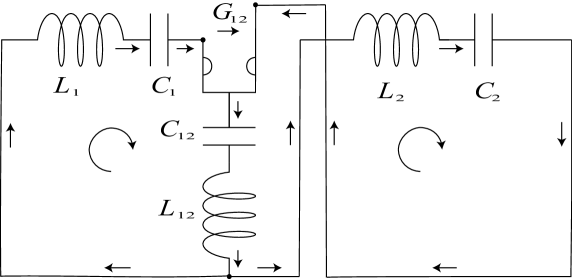
Figure 1.1. The network of two oriented $LC$-loops that are coupled by $GLC$-link. The link is composed of ($k$) a gyrator of the gyrator resistance $G_{12}$, (ii) a capacitor of the capacitance $C_{12}$ and (iii) an inductor of inductance $L_{12}$ connected in a series. The values of involved elements are defined by equations (1.6) and (1.7). Notice the difference between the left and the right connections for the gyrator and $LC$-loops. It is explained by the non-reciprocity of the gyrator and is designed to be consistent with (i) the standard port assignment and selection of positive directions for the loop currents and the gyrator; (ii) the sign of gyration resistance as shown in Fig. 4.2 and equations (4.2).

A simple procedure for the construction of the canonical $GLC$-loop Lagrangian form of the original general quadratic Lagrangian is provided in Section 2. This canonical $GLC$-loop Lagrangian leads straightforwardly to the synthesis of the canonical $GLC$-network associated with the Lagrangian.

2. Preparation to the circuit synthesis

We are interested in lossless circuits, that is there no resistors are involved. We name such circuits $GLC$-circuits and define them as follows.

Definition 1 ($GLC$-circuit).

$GLC$-circuit is defined as any circuit composed of (i) capacitors and inductors of positive or negative values for the respective capacitances and inductances; (ii) gyrators.

Let the Lagrangian be of general quadratic form

(2.1) $$\mathcal{L}=\frac{1}{2}\dot{Q}^{\mathrm{T}}\alpha\dot{Q}+\dot{Q}^{\mathrm{T}}\theta Q-\frac{1}{2}Q^{\mathrm{T}}\eta Q,\quad\dot{Q}=\partial_{t}Q,\quad Q=\left[Q_{1},Q_{2},\ldots,Q_{N}\right]{}^{\mathrm{T}},$$

or

(2.2) $$\mathcal{L}=\frac{1}{2}\sum_{k,m=1}^{N}\alpha_{km}\dot{Q}_{k}\dot{Q}_{m}+\sum_{k,m=1}^{N}\theta_{km}Q_{m}\dot{Q}_{k}-\frac{1}{2}\sum_{k,m=1}^{N}\eta_{km}Q_{k}Q_{m},$$

where $\alpha=\left\{\alpha_{km}\right\}$, $\theta=\left\{\theta_{km}\right\}$ and $\eta=\left\{\eta_{km}\right\}$ are $N\times N$ matrices satisfying

(2.3) $$\alpha_{km}=\alpha_{mk},\quad\theta_{km}=-\theta_{mk},\quad\eta_{km}=\eta{}_{mk},\quad 1\leq k,m\leq N.$$

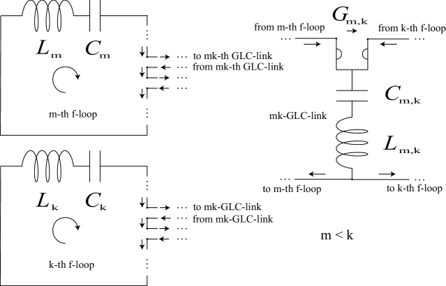
Figure 2.1. This figure provides graphical support to the circuit synthesis by showing how the $m$-th and the $k$-th f-loops are coupled by the $GLC$-link of the index $m,k$. It is understood that any other pair of f-loops can be coupled if needed similarly. Notice that under assumption $m<k$ the $m$-th and $k$-th f-loop are connected respectively to the left and to right shoulders of $GLC$-link. The arrows indicate the positive directions of the currents. All shown connections are designed to be consistent with (i) the standard port assignment and selection of positive directions for the loop currents and the gyrator; (ii) the sign of gyration resistance as shown in Fig. 4.2 and equations (4.2).

The first step of the circuit synthesis based on the prescribed Lagrangian defined by equations (2.1) - (2.3) is to transform it into a particular form suited for its circuit implementation. This transformation starts with the interpretation of the coordinates $Q_{m}$ and the corresponding generalized velocities $v_{m}=\partial_{t}Q_{m}$, $1\leq m\leq N$ as respectively the $m$-th f-loop charges and currents of the circuit to be constructed. With this interpretation in mind the terms $\frac{1}{2}\alpha_{mm}\dot{Q}_{m}^{2}$ and $\frac{1}{2}\eta_{mm}Q_{m}^{2}$ can be naturally attributed respectively to the energies of an inductor of the inductance $L_{m}=\alpha_{mm}$ and a capacitor of the inverse capacitance $B_{m}=C_{m}^{-1}=\eta_{mm}$ associated with $m$-th f-loop. The terms $\frac{1}{2}\alpha_{km}\dot{Q}_{k}\dot{Q}_{m}$ and $\frac{1}{2}\eta_{km}Q_{k}Q_{m}$ for $k\neq m$ are commonly attributed respectively to the energies of mutual inductance $L_{km}=\alpha_{km}$ and mutual capacitance of the inverse capacitance $B_{km}=C_{km}^{-1}=\eta_{mm}$. Though these terms evidently carry information on mutual coupling between different f-loops they are not linked directly to branches of a circuit. To address the problem we use elementary identity $2ab=\left(a+b\right)^{2}-a^{2}-b^{2}$ for $a=Q_{k},\dot{Q}_{k}$ and $b=Q_{m},\dot{Q}_{m}$ and rearrange the Lagrangian terms as follows

(2.4) $$\frac{1}{2}\sum_{k,m=1}^{N}\alpha_{km}\dot{Q}_{k}\dot{Q}_{m}=\frac{1}{2}\sum_{k=1}^{N}\left(2\alpha_{kk}-\sum_{m=1}^{N}\alpha_{km}\right)\dot{Q}_{k}^{2}+\frac{1}{2}\sum_{1\leq m<k\leq N}\alpha_{km}\left(\dot{Q}_{k}+\dot{Q}_{m}\right)^{2}.$$

(2.5) $$\frac{1}{2}\sum_{k,m=1}^{N}\eta_{km}Q_{k}Q_{m}=\frac{1}{2}\sum_{k=1}^{N}\left(2\eta_{kk}-\sum_{m=1}^{N}\eta_{km}\right)Q_{k}^{2}+\frac{1}{2}\sum_{1\leq m<k\leq N}\left(Q_{k}+Q_{m}\right)^{2},$$

Notice also

(2.6) $$\sum_{k,m}\theta_{km}Q_{m}\dot{Q}_{k}=\sum_{1\leq m<k\leq N}\theta_{km}\left(Q_{m}\dot{Q}_{k}-Q_{k}\dot{Q}_{m}\right).$$

Based on identities (2.4)-(2.6) we recast the original Lagrangian defined by equations (2.1)-(2.3) as

(2.7) $$\mathcal{L}=\sum_{k=1}^{N}\mathcal{L}_{k}+\sum_{1\leq m<k\leq N}\mathcal{L}_{km},$$

(2.8) $$\mathcal{L}_{k}=L_{k}\dot{Q}_{k}^{2}+B_{k}Q_{k}^{2},\;\dot{Q}_{k}=\partial_{t}\left(Q\right),\;1\leq k\leq N,$$

(2.9) $$\mathcal{L}_{km}=L_{km}\left(\dot{Q}_{k}+\dot{Q}_{m}\right)^{2}+B_{km}\left(Q_{k}+Q_{m}\right)^{2}+G_{km}\left(Q_{m}\dot{Q}_{k}-Q_{k}\dot{Q}_{m}\right),\;1\leq m<k\leq N,$$

where inductances $L_{k}$ and $L_{km}$, inverse capacitances $B_{k}$ and $B_{km}$, and gyration resistances $G_{km}$ are defined by

(2.10) $$L_{k}=2\alpha_{kk}-\sum_{m=1}^{N}\alpha_{km}=\alpha_{kk}-\sum_{m\neq k}\alpha_{km},\quad 1\leq k\leq N;$$

(2.11) $$L_{km}=\alpha_{km},\quad 1\leq m<k\leq N;$$

(2.12) $$B_{k}=C_{k}^{-1}=2\eta_{kk}-\sum_{m=1}^{N}\eta_{km}=\eta_{kk}-\sum_{m\neq k}\eta_{km},\quad 1\leq k\leq N;$$

(2.13) $$B_{km}=C_{km}^{-1}=\eta{}_{km},\quad G_{km}=\theta_{km},\quad 1\leq m<k\leq N,$$

We refer to the Lagrangian representation (2.7)-(2.9) as the loop Lagrangian. The point of the above transformation leading to the loop Lagrangian is to replace products $\dot{Q}_{k}\dot{Q}_{m}$ and $Q_{k}Q_{m}$ with respectively $\left(\dot{Q}_{k}+\dot{Q}_{m}\right)^{2}$ and $\left(Q_{k}+Q_{m}\right)^{2}$ accompanied by the proper modification of the coefficients before $\dot{Q}_{k}^{2}$ and $Q_{m}^{2}$. With that done we notice first that the Lagrangian $\mathcal{L}_{k}$ defined by equations (2.8) can naturally be associated with $k$-th f-loop of the circuit to be constructed, see Section 4.1 and equations (4.11), (4.12) there. As to the Lagrangian $\mathcal{L}_{km}$ defined by equations (2.9) it is perfectly suited to be attributed to what we call a $GLC$-link which is a connector between $k$-th and $m$-th f-loops defined as follows.

Definition 2 ($GLC$-link).

$GLC$-link, shown on the right side of Fig. 2.1, is a branch composed of a circuit made of (i) a gyrator of the gyrator resistance $G$, (ii) a capacitor of the capacitance $C$ and (iii) an inductor of inductance $L$ connected in a series. Some of the quantities $G$, $B=C^{-1}$and $L$ are allowed to be zero but at least one them is required to be non-zero. In other words, $GLC$-link can be composed of 3, 2 or 1 elements. For instance, it can just a gyrator or capacitor, or it can be a combination of a capacitor and inductance.

Indeed, equations (2.9) suggest that the charge and the corresponding current associated with the $GLC$-link are respectively $Q_{k}+Q_{m}$ and $\partial_{t}\left(Q_{k}+Q_{m}\right)$ and the gyroscopic interaction between $k$-th and $m$-th f-loops is accounted for by the term involving gyration resistances $G_{km}$.

Notice that it might happen that for particular values of indexes $\mathcal{L}_{k}=0$ and/or $\mathcal{L}_{km}=0$, implying effectively that the corresponding circuit elements have to be eliminated. In particular, the possibility of $\mathcal{L}_{km}=0$ can result in a circuit which is a composition of two or more totally disconnected components. In view of these factors we want to limit naturally our considerations to Lagrangians that yield connected circuits only. With that in mind we introduce the concepts of connected f-loops and of admissible Lagrangian as follows.

Definition 3 (connected f-loops).

Using the expressions (2.9) for the Lagrangian component $\mathcal{L}_{km}$ valid for $1\leq m<k\leq N$ we define $\mathcal{L}_{km}$ for every pair $k\neq m$ by the following equality

(2.14) $$\mathcal{L}_{km}=\mathcal{L}_{sp},\;s=\min\left\{k,m\right\},\;p=\max\left\{k,m\right\}.$$

We define then for $k\neq m$ the $k$-th and the $m$-th f-loops to be directly connected if $\mathcal{L}_{km}\neq 0$. For $k\neq m$ the $k$-th and the $m$-th f-loops are called connected if the following is true. There exists a set $S_{km}=\left\{s_{1},\ldots,s_{q}\right\}$ of distinct indexes $s_{i}\neq k,m$ such that for every pair $\left\{s_{i},s_{i+1}\right\}$ the corresponding f-loops are directly connected for $0\leq i\leq q$ assuming that $s_{0}=k$ and $s_{q+1}=m$. In other words, the $k$-th and the $m$-th f-loops are connected if there exists a “path” from $k$ to $m$ in the set of indexes such the end points of each of its segments correspond to directly connected f-loops.

Having defined connected f-loops we proceed with the following definition.

Definition 4 (admissible Lagrangian).

We refer to the loop Lagrangian defined by equations (2.7)-(2.9) as admissible if (i) for every pair of different indexes $\left\{k,m\right\}$ corresponding f-loops are connected; (ii) every $k$-th f-loop Lagrangian $\mathcal{L}_{k}$ defined by equations (2.7) and (2.8) is not zero, that is

(2.15) $$\mathcal{L}_{k}\neq 0,\;1\leq k\leq N.$$

3. The circuit synthesis

The circuit synthesis described in this sections is based on the results of Section 2. It assumes that: (i) the Lagrangian is admissible according to Definition 4, and (ii) the synthesized circuit is an $GLC$-circuit as in Definition 1. In fact, the synthesis process is rather straightforward and guided by Fig. 2.1 providing visual support. We still add to that formal steps of the synthesis algorithm to make sure that the synthesized $GLC$-circuit implements the desired goals.

The circuit synthesis algorithm can be viewed a process of consequent modifications of the set of initially isolated f-loops as they get connected by proper $GLC$-links. The process utilizes the expressions of the loop Lagrangian components $\mathcal{L}_{k}$ and $\mathcal{L}_{km}$ defined by equations (2.7)-(2.9) and its steps are as follows.

The circuit synthesis algorithm.

1. Set up the initial state of the f-loops. Based on the Lagrangians $\mathcal{L}_{k}$, $1\leq k\leq N$ we create the corresponding $LC$-circuits (f-loops) $\mathsf{F}_{k}$ with the values of inductances $L_{k}$ and capacitances $C_{k}$ defined by equations (2.10) and (2.12). These initially disconnected f-loops $\mathsf{F}_{k}$ constitute the initial state of circuit before the their coupling process is fully implemented.

2. Create the $GLC$-links to be used for coupling of the f-loops. Based on non-zero Lagrangians $\mathcal{L}_{km}$, $1\leq m<k\leq N$ we create $GLC$-links $\mathsf{G}_{km}$ with the values of inductances $L_{km}$, capacitances $C_{km}$ and gyration resistances $G_{km}$ defined by equations (2.11) and (2.13).

3. Modify recurrently f-loops $\mathsf{F}_{k}$ by coupling them with $GLC$-links $\mathsf{G}_{km}$. The modification process starts with the initial state of the f-loops $\mathsf{F}_{k}$. Its goal is to add up to the initial state of the $GLC$-circuit one-by-one all non-zero $GLC$-links $\mathsf{G}_{km}$. Suppose that $\mathsf{F}_{m}^{\prime}$ and $\mathsf{F}_{k}^{\prime}$ for $m<k$ constitute an intermediate state of the $m$-th and $k$-th loops in the process of adding non-zero $GLC$-links. We modify them by adding up $GLC$-link $\mathsf{G}_{km}$ as follows. We open up the f-loop $\mathsf{F}_{m}^{\prime}$ by removing its wire segment and connect the ends of the so open f-loop to the left shoulder of $GLC$-link $\mathsf{G}_{km}$ as indicated in Fig. 2.1. Then we open up the f-loop $\mathsf{F}_{k}^{\prime}$ by removing its wire segment and connect the ends of the so open f-loop to the right shoulder of $GLC$-link $\mathsf{G}_{km}$ as indicated in Fig. 2.1. As the result of the modification we get new states $\mathsf{F}_{m}^{\prime\prime}$ and $\mathsf{F}_{k}^{\prime\prime}$ for the corresponding f-loops with integrated into them $GLC$-link $\mathsf{G}_{km}$. Executing the described process until all $GLC$-links $\mathsf{G}_{km}$ are integrated into the $GLC$-circuit we arrive at the desired synthesized circuit.

It follows from the circuit synthesis algorithm that the synthesized $GLC$-circuit is uniquely defined by the prescribed Lagrangian. This circuit can be viewed as canonical and we name it canonical $GLC$-circuit. Since any $GLC$-circuit can be associated with the Lagrangian based on equations (4.11) and (4.11) for its elementary terms the following statements hold.

Theorem 5 (circuit implementation of a Lagrangian system).

Any finite-dimensional physical system described by a Lagrangian can be implemented as the canonical $GLC$-circuit associated with it.

Theorem 6 (equivalent canonical $GLC$-circuit).

Any $GLC$-circuit has an equivalent representation as the canonical $GLC$-circuit in the sense that the evolution equations for the both circuits are equivalent.

A $GLC$-circuit can be different from its canonical $GLC$-circuit. This is the case when the circuit has a twig which is common to more than two loops as demonstrated below by an example of simple $GLC$-circuit that involves only inductors and capacitors.

Example 7 (canonical $GLC$-circuit).

Let us consider a circuit composed of 3 f-loops with inductances and inverse capacitances respectively $L_{k},B_{k}$,$\>k=1,2,3$ and having a single common branch with inductances and inverse capacitances respectively $L_{b},B_{b}$. The corresponding circuit Lagrangian then is

(3.1) $$\mathcal{L}=\frac{1}{2}\sum_{k=1}^{3}\left(L_{k}\dot{Q}_{k}^{2}-B_{k}Q_{k}^{2}\right)+\frac{L_{\mathrm{b}}}{2}\left(\dot{Q}_{1}+\dot{Q}_{2}+\dot{Q}_{3}\right)^{2}-\frac{B_{\mathrm{b}}}{2}\left(Q_{1}+Q_{2}+Q_{3}\right)^{2}.$$

Then according to equations (2.10), (2.12), (2.11) and (2.13) the canonical $GLC$-circuit involves only inductors and capacitors of the following respective values for inductances and inverse capacitances

(3.2) $$\mathring{L}_{k}=L_{k}-L_{\mathrm{b}},\quad\mathring{B}_{k}=B_{k}-B_{\mathrm{b}},\quad k=1,2,3,$$

(3.3) $$\mathring{L}_{km}=L_{\mathrm{b}},\quad\mathring{B}_{mk}=B_{\mathrm{b}},\quad 1\leq m<k\leq 3.$$

Notice that if the values of all inductances and capacitances of the original circuit are positive, that is $L_{k},L_{\mathrm{b}}>0,B_{k},B_{\mathrm{b}}>0$,$\>k=1,2,3$ then according to equations (3.2) and (3.3) some of the corresponding values $\mathring{L}_{k}$ and $\mathring{B}_{k}$ for the canonical $GLC$-circuit can evidently be negative.

4. A Sketch of the Basics of Electric Networks

For the sake of self-consistency, we provide in this section basic information on the basics of the electric network theory and relevant notations.

Electrical networks is a well established subject represented in many monographs. We present here basic elements of the electrical network theory following mostly to [BalBic, 2], [Cau], [SesRee]. The electrical network theory constructions are based on the graph theory concepts of branches (edges), nodes (vertices) and their incidences. This approach is efficient in loop (fundamental circuit) analysis and the determination of independent variables for the Kirchhoff current and voltage laws - the subjects relevant to our studies here.

We are particularly interested in conservative electrical network which is a particular case of an electrical network composed of electric elements of three types: capacitors, inductors and gyrators. We remind that a capacitor or an inductor are the so-called two-terminal electric elements whereas a gyrator is four-terminal electric element as discussed below. We assume that capacitors and inductors can have positive or negative respective capacitances and inductances.

4.1. Circuit elements and their voltage-current relationships

The elementary electric network (circuit) elements of interest here are a capacitor, an inductor, a resistor and a gyrator, [BalBic, 1.5, 2.6], [Cau, App.5.4], [Iza, 10]. These elements are characterized by the relevant voltage-current relationships. These relationships for the capacitor, inductor and resistor are respectively as follows [BalBic, 1.5], [Rich, 3-Circuit theory], [SesBab, 1.3]:

(4.1) $$I=C\partial_{t}V,\quad V=L\partial_{t}I,\quad V=RI,$$

where $I$ and $V$ are respectively the current and the voltage, and real $C$, $L$ and $R$ are called respectively the capacitance, the inductance and the resistance. The voltage-current relationship for the gyrator depicted in Fig. 4.2 are

(4.2) $$(a):\>\begin{bmatrix}V_{1}\\ V_{2}\end{bmatrix}=\begin{bmatrix}-GI_{2}\\ GI_{1}\end{bmatrix},\quad(b):\>\begin{bmatrix}V_{1}\\ V_{2}\end{bmatrix}=\begin{bmatrix}GI_{2}\\ -GI_{1}\end{bmatrix},$$

where $I_{1},\>I_{2}$ and $V_{1},\>V_{2}$ are respectively the currents and the voltages, and quantity $G$ is called the gyration resistance.

The common graphic representations of the network elements are depicted in Figs. 4.1 and 4.2. The arrow next to the symbol $G$ in Fig. 4.2 shows the direction of gyration.

The gyrator has the so-called inverting property as shown in Fig. 4.3, [BalBic, 1.5], [Dorf, 29.1], [Iza, 10]. Namely, when a capacitor or an inductor connected to the output port of the gyrator it behaves as an inductor or capacitor respectively with the following effective values

(4.3) $$L_{\mathrm{ef}}=G^{2}C,\quad C_{\mathrm{ef}}=\frac{L}{G^{2}}.$$

Notice that the voltage-current relationships in equations (4.2) (b) can be obtained from the same in equations (4.2) (a) by substituting $-G$ for $G$. The gyrator is a device that accounts for physical situations in which the reciprocity condition does not hold. The voltage-current relationships in equations (4.2) show that the gyrator is a non-reciprocal circuit element. In fact, it is antireciprocal. Notice, that the gyrator, like the ideal transformer, is characterized by a single parameter $G$, which is the gyration resistance. The arrows next to the symbol $G$ in Fig. 4.2(a) and (b) show the direction of gyration.

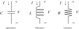
Figure 4.1. Capacitance, inductance and resistance.

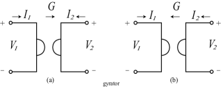
Figure 4.2. Gyrator.

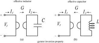
Figure 4.3. (a) Effective inductor; (b) effective capacitor.

Along with the voltage $V$ and the current $I$ variables we introduce the charge variable $Q$ and the momentum (per unit of charge) variable $P$ by the following formulas

(4.4) $$Q\left(t\right)=\intop I\left(t\right)\,dt,\quad I\left(t\right)=\partial_{t}Q,$$

(4.5) $$P\left(t\right)=\intop V\left(t\right)\,dt,\quad V\left(t\right)=\partial_{t}P.$$

We introduce also the energy stored variable $W$, [Rich, Circuit Theory]. Then the voltage-current relations (4.1) and the stored energy $W$ can be represented as follows:

(4.6) $$\text{capacitor: }V=\frac{Q}{C},\quad I=\partial_{t}Q=C\partial_{t}V,$$

$$Q=CV=C\partial_{t}P;$$

(4.7) $$W=\frac{1}{2}VQ=\frac{Q^{2}}{2C}=\frac{CV^{2}}{2}=\frac{C\left(\partial_{t}P\right)^{2}}{2};$$

(4.8) $$\text{inductor: }V=L\partial_{t}I,\quad P=LI=L\partial_{t}Q,$$

$$\partial_{t}Q=\frac{P}{L};$$

(4.9) $$W=\frac{PI}{2}=\frac{LI^{2}}{2}=\frac{L\left(\partial_{t}Q\right)^{2}}{2}=\frac{P^{2}}{2L};$$

(4.10) $$\text{resistor: }V=RI,\quad P=RQ.$$

The Lagrangian associated with the network elements are as follows [GantM, 9], [Rich, 3]:

(4.11) $$\text{capacitor: }\mathcal{L}=\frac{Q^{2}}{2C},\>\text{inductor: }\mathcal{L}=\frac{L\left(\partial_{t}Q\right)^{2}}{2},$$

(4.12) $$\text{gyrator: }\mathcal{L}=GQ_{1}\partial_{t}Q_{2},$$

$$\mathcal{L}=\frac{G\left(Q_{1}\partial_{t}Q_{2}-Q{}_{2}\partial_{t}Q_{1}\right)}{2}.$$

Notice that the difference between two alternatives for the Lagrangian in equations (4.12) is $\frac{1}{2}G\partial_{t}\left(Q_{1}Q_{2}\right)$ which is evidently the complete time derivative. Consequently, the EL equation are the same for both Lagrangians, see Section 6.

4.2. Circuits of negative impedance, capacitance and inductance

There is a number of physical devices that can provide for negative capacitances and inductances needed for our circuits [Dorf, 29]. Figure 4.4 shows operational amplifiers that implement negative impedance, capacitance and inductance respectively, Following to [Iza, 10].

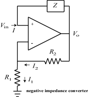
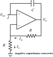
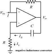
(a)                                           (b)                                           (c)

Figure 4.4. Operational-amplifier-based negative (a) impedance converter; (b) capacitance converter; (c) inductance converter.

The currents and voltages for circuits depicted in Fig. 4.4 are respectively as follows: (i) for negative impedance as in Fig. 4.4(a)

(4.13) $$V_{\mathrm{in}}=-ZI,\quad V_{\mathrm{o}}=2V_{\mathrm{in}},\quad I_{1}=I_{2}=\frac{V_{\mathrm{in}}}{R};$$

(ii) for negative capacitance as in Fig. 4.4(b)

(4.14) $$V_{\mathrm{in}}=Z_{\mathrm{in}}I,\quad Z_{\mathrm{in}}=-\frac{\mathrm{i}}{\omega C},\quad V_{\mathrm{o}}=2V_{\mathrm{in}},\quad I_{1}=I_{2}=\frac{V_{\mathrm{in}}}{R};$$

(iii) for negative inductance as in Fig. 4.4(c)

(4.15) $$V_{\mathrm{in}}=Z_{\mathrm{in}}I,\quad Z_{\mathrm{in}}=-\mathrm{i}\omega R^{2}C,\quad I_{1}=I_{2}=\frac{V_{\mathrm{in}}}{R},\quad V_{\mathrm{o}}=V_{\mathrm{in}}\left(1+\frac{1}{\mathrm{i}\omega RC}\right).$$

4.3. Topological aspects of the electric networks

We follow here mostly to [BalBic, 2]. The purpose of this section is to concisely describe and illustrate relevant concepts with understanding that the precise description of all aspects of the concepts is available in [BalBic, 2].

To describe topological (geometric) features of the electric network we use the concept of linear graph defined as a collection of points, called nodes, and line segments called branches, the nodes being joined together by the branches as indicated in Fig. 4.2 (b). Branches whose ends fall on a node are said to be incident at the node. For instance, Fig. 4.2 (b) branches 1, 2, 3, 4 are incident at node 2. Each branch in Fig. 4.2 (b) carries an arrow indicating its orientation. A graph with oriented branches is called an oriented graph. The elements of a network associated with its graph have both a voltage and a current variable, each with its own reference. In order to relate the orientation of the branches of the graph to these references the convention is made that the voltage and current of an element have the standard reference - voltage-reference “plus” at the tail of the current-reference arrow. The branch orientation of a graph is assumed to coincide with the associated current reference as shown in Figures 4.1 and 4.2.

We denote the number of branches of the network by $N_{\mathrm{b}}\geq 2$, and the number of nodes by $N_{\mathrm{n}}\geq 2$.

A subgraph is a subset of the branches and nodes of a graph. The subgraph is said to be proper if it consists of strictly less than all the branches and nodes of the graph. A path is a particular subgraph consisting of an ordered sequence of branches having the following properties:

1. At all but two of its nodes, called internal nodes, there are incident exactly two branches of the subgraph.

2. At each of the remaining two nodes, called the terminal nodes, there is incident exactly one branch of the subgraph.

3. No proper subgraph of this subgraph, having the same two terminal nodes, has properties 1 and 2.

A graph is called connected if there exists at least one path between any two nodes. We consider here only connected graphs such as shown in Fig. 4.5 (b).

A loop (cycle) is a particular connected subgraph of a graph such that at each of its nodes there are exactly two incident branches of the subgraph. Consequently, if the two terminal nodes of a path coincide we get a “closed path”, that is a loop. In Fig. 4.5 (b) branches 7, 1, 3, 5 together with nodes 1, 2, 3, and 4 form a loop. We can specify a loop by an either the ordered list of the relevant branched or the ordered list of the relevant nodes.

We remind that each branch of the network graph is associated with two functions of time $t$: its current $I(t)$ and its voltage $V(t)$. The set of these functions satisfy two Kirchhoff’s laws, [BalBic, 2.2], [Cau, 2], [Rich, Circuit Theory], [SesRee, 1]. The Kirchhoff current law (KCL) states that in any electric network the sum of all currents leaving any node equals zero at any instant of time. The Kirchhoff voltage law (KVL) states that in any electric network, the sum of voltages of all branches forming any loop equals zero at any instant of time. It turns out that the number of independent KCL equations is $N_{\mathrm{n}}-1$ and the number KVL equations is $N_{\mathrm{fl}}=N_{\mathrm{b}}-N_{\mathrm{n}}+1$ (the first Betti number [Cau, 2], [SesRee, 2.3]).

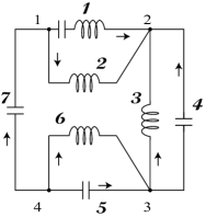
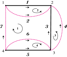
(a)                                                        (b)

Figure 4.5. The network (a) and its graph (b). There are $4$ nodes marked by small disks (black). In (b) there are $3$ twigs identified by bolder (black) lines and labeled by numbers 1, 3, 5. There are $4$ links identified by dashed (red) lines and labeled by numbers 2, 4, 6, 7. There also $4$ oriented f-loops formed by the branches as shown.

There is an important concept of a tree in the network graph theory [BalBic, 2.2], [Cau, 2.1] and [SesRee, 2.3]. A tree, known also as complete tree, is defined as a connected subgraph of a connected graph containing all the nodes of the graph but containing no loops as illustrated in Fig. 4.5 (b). The branches of the tree are called twigs and those branches that are not on a tree are called links [BalBic, 2.2]. The links constitute the complement of the tree, or the cotree. The decomposition of the graph into a tree and cotree is not a unique.

The system of fundamental loops or system of f-loops for short, [BalBic, 2.2], [Cau, 2.1] and [SesRee, 2.3], is of particular importance to our studies. The system of time-dependent charges (defined as the time integrals of the currents) associated with the system of f-loops provides a complete set of independent variables. When the network tree is selected then every link defines the containing it f-loop. The orientation of an f-loop is defined by the orientation of the link it contains. Consequently, there are as many of f-loops in as there are links, and

(4.16) $$\text{number of $f$-loops}:\;N_{\mathrm{fl}}=N_{\mathrm{b}}-N_{\mathrm{n}}+1.$$

The number $N_{\mathrm{fl}}$ of f-loops defined by equation (4.16) quantifies the connectivity of the network graph, and it is known in the algebraic topology as the first Betti number [Cau, 2], [SesRee, 2.3]), [Witt].

The discussed concepts of the graph of an electric network such as the tree, twigs, links and f-loops are illustrated in Fig. 4.5. In particular, there are $4$ nodes marked by small disks (black). In Fig. 4.5 (b) there are $3$ twigs identified by bolder (black) lines and labeled by numbers 1, 3, 5. There are $4$ links identified by dashed (red) lines and labeled by numbers 2, 4, 6, 7. There also $4$ oriented f-loops formed by the branches as follows: (1) 7, 1, 3, 5; (2) 2, 1; (3) 4, 3; (2) 6, 5. These representations of the f-loops as ordered lists of branches identify the corresponding links as number in the first position in every list.

One also distinguishes simpler planar networks with graphs that can be drawn so that lines representing branches do not intersect. The graph of a general electric network does not have to be planar though. Networks with non-planar graphs can still be represented graphically with more complex display arrangements or algebraically by the incidence matrices, [BalBic, 2.2].

5. Conclusions

We developed here an algorithm of a synthesis of a lossless electric circuit based on prescribed Lagrangian. This means that the electric circuit evolution equations are equivalent to the relevant Euler-Lagrange equations. The synthesized circuit is composed of (i) capacitors and inductors of positive or negative values for respective capacitances and inductances, and (ii) gyrators. The proposed synthesis can be viewed as a systematic approach in a realization of any finite dimensional physical system described by a Lagrangian in a lossless electric circuit.

The synthesis can be used in a number of ways. It can be used to realize the desired spectral properties in an electric circuit through a Lagrangian that carries the properties directly. It can be also used in the realization of arbitrary mutual capacitances and inductances in terms of elementary capacitors and inductors of positive and negative respective capacitances and inductances. The synthesis can be utilized also to generate circuit approximations to transmission lines and waveguides within the frequency limitations.

Acknowledgment: This research was supported by AFOSR grant # FA9550-19-1-0103 and Northrop Grumman grant # 2326345.

We are grateful to Prof. F. Capolino, University of California at Irvine, for reading the manuscript and giving valuable suggestions.

Data sharing is not applicable to this article as no data sets were generated or analyzed during the current study.

6. Appendix: Concise review of the Lagrangian formalism

Following common practice in the circuit theory, we assume the circuit system configuration to be described by $N$-dimensional vector-columns of voltages $V(z,t)=\left\{V_{s}(z,t)\right\}_{s=1,\ldots,N}$ and currents $I(z,t)=\left\{I_{s}(z,t)\right\}_{s=1,\ldots,N}$. Our primary circuit variables though are $N$-dimensional vector-column of charges

(6.1) $$Q(z,t)=\left\{Q_{s}(z,t)\right\}_{s=1,\ldots,N},\quad Q_{s}(z,t)=\int^{t}I_{s}(z,t^{\prime})\,\mathrm{d}t^{\prime}.$$

The Lagrangian $\mathcal{L}$ for a linear system is a quadratic function (bilinear form) of the system state $Q=\left[q_{r}\right]_{r=1}^{n}$ (column vector) and its time derivatives $\partial_{t}Q$, that is

(6.8) $$\mathcal{L}=\mathcal{L}\left(Q,\partial_{t}Q\right)=\frac{1}{2}\left[\begin{array}[]{l}Q\\ \partial_{t}Q\end{array}\right]^{\mathrm{T}}M_{\mathrm{L}}\left[\begin{array}[]{l}Q\\ \partial_{t}Q\end{array}\right],\quad M_{\mathrm{L}}=\left[\begin{array}[]{rr}-\eta&\theta^{\mathrm{T}}\\ \theta&\alpha\end{array}\right],$$

where $\mathrm{T}$ denotes the matrix transposition operation, and $\alpha,\eta$ and $\theta$ are $n\times n$-matrices with real-valued entries. In addition to that, we assume matrices $\alpha,\eta$ to be symmetric, that is

(6.9) $$\alpha=\alpha^{\mathrm{T}},\qquad\eta=\eta^{\mathrm{T}}.$$

Consequently,

(6.10) $$\mathcal{L}=\frac{1}{2}\partial_{t}Q^{\mathrm{T}}\alpha\partial_{t}Q+\partial_{t}Q^{\mathrm{T}}\theta Q-\frac{1}{2}Q^{\mathrm{T}}\eta Q.$$

Then by Hamilton’s principle, the system evolution is governed by the EL equations

(6.11) $$\frac{d}{dt}\left(\frac{\partial\mathcal{L}}{\partial\partial_{t}Q}\right)-\frac{\partial\mathcal{L}}{\partial Q}=0,$$

which, in view of equation (6.10) for the Lagrangian $\mathcal{L}$, turns into the following second-order vector ordinary differential equation (ODE):

(6.12) $$\alpha\partial_{t}^{2}Q+\left(\theta-\theta^{\mathrm{T}}\right)\partial_{t}Q+\eta Q=0.$$

Notice that matrix $\theta$ enters equation (6.12) through its skew-symmetric component $\frac{1}{2}\left(\theta-\theta^{\mathrm{T}}\right)$ justifying as a possibility to impose the skew-symmetry assumption on $\theta$, that is

(6.13) $$\theta^{\mathrm{T}}=-\theta.$$

Indeed, the symmetric part $\theta_{s}=\frac{1}{2}\left(\theta+\theta^{\mathrm{T}}\right)$ of the matrix $\theta$ is associated with a term to the Lagrangian which can be recast as is the complete (total) derivative, namely $\frac{1}{2}\partial_{t}\left(Q^{\mathrm{T}}\theta_{s}Q\right)$. It is a well known fact that adding to a Lagrangian the complete (total) derivative of a function of $Q$ does not alter the EL equations. Namely, the EL equations are invariant under the Lagrangian gauge transform $\mathcal{L}\rightarrow\mathcal{L}+\partial_{t}F\left(q,t\right)$, [Scheck, 2.9, 2.10], [LanLifM, I.2].

Under the assumption (6.13) equation (6.12) turns into its version with the skew-symmetric $\theta$

(6.14) $$\alpha\partial_{t}^{2}Q+2\theta\partial_{t}Q+\eta Q=0,\text{ if }\theta^{\mathrm{T}}=-\theta.$$

It turns out though that the Lagrangian that corresponds to the Hamiltonian by the Legendre transformation does not have to have skew-symmetric $\theta$ satisfying (6.13). For this reason we don’t impose the condition of skew-symmetry on $\theta$.

6.1. Lagrangian framework for an electric network

The possibility of the construction of the Lagrangian framework for electric circuits is well known. Basic examples of such a construction are provided, for instance, in [GantM, 9], [Wells, 15], The well-known expressions for the Lagrangian for the basis circuit elements considered in Section 4.1 are as follows [GantM, 9], [Rich, 3]:

(6.15) $$\text{capacitance: }\mathcal{L} =-\frac{\left(Q\right)^{2}}{2C},$$

(6.16) $$\text{inductance: }\mathcal{L} =\frac{L\left(\partial_{t}Q\right)^{2}}{2},$$

(6.17) $$\text{gyrator: }\mathcal{L} =\frac{G}{2}\left(Q_{1}\partial_{t}Q_{2}-Q_{2}\partial_{t}Q_{1}\right),$$

Suppose now that we have a lossless circuit composed of capacitors, inductors and gyrators of positive or negative values for the respective capacitances and inductances. There is a well defined procedure (algorithm) that allows to assign to such a circuit a Lagrangian. This procedure is as follows.

The first immediate question as we start the construction of the circuit Lagrangian is what is the set of independent variables describing the state of the circuit at any point of time? To answer this question we use the results of Section 4.3 and identify a circuit tree and the corresponding set of f-loops. With that been done we introduce the charges $Q_{m}$ and the currents $\partial_{t}Q_{m}$, $1\leq m\leq N$ associated the corresponding $N$ f-loops to be the generalized coordinates defining the state of the circuit at any point of time.

Then the process of generating the circuit Lagrangian $\mathcal{L}$ follows to the following steps.

1. If $\mathrm{b}$ is a link, see the definition in Section 4.3, associated with the f-loop of the index $m=m\left(\mathrm{b}\right)$ then it is associated with either capacitance $C_{\mathrm{b}}$ or inductance $L_{\mathrm{b}}$ and is assigned respectively according to equations (6.15) and (6.16) the following value of the Lagrangian

   (6.18) $$\mathcal{L}_{\mathrm{b}}=\frac{Q_{m}^{2}}{2C_{\mathrm{b}}},\quad\mathcal{L}_{\mathrm{b}}=\frac{L_{\mathrm{b}}\left[\partial_{t}Q_{m}\right]^{2}}{2},\;m=m\left(\mathrm{b}\right).$$

2. If $\mathrm{b}$ is a twig, see the definition in Section 4.3, we consider the set $S\left(\mathrm{b}\right)$ of indexes $m$ of f-loops containing the twig $\mathrm{b}$. To account for mutual orientations of branches and f-loops and consequently the signs of f-loop currents we introduce for any $m\in S\left(\mathrm{b}\right)$ the corresponding $\epsilon\left(m\right)=\pm 1$ as follows. If the orientations of the twig $\mathrm{b}$ and the $m$-th f-loop that includes it are the same we set $\epsilon\left(m\right)=1$, otherwise $\epsilon\left(m\right)=-1$. If the twig is associated with either capacitance $C_{\mathrm{b}}$ or inductance $L_{\mathrm{b}}$ we assign to it respectively the following Lagrangian

   (6.19) $$\mathcal{L}_{\mathrm{b}}=\frac{Q_{\mathrm{b}}^{2}}{2C_{\mathrm{b}}},\quad\mathcal{L}_{\mathrm{b}}=\frac{L_{\mathrm{b}}\left[\partial_{t}Q_{\mathrm{b}}\right]^{2}}{2},\quad Q_{\mathrm{b}}=\sum_{m\in S\left(\mathrm{b}\right)}\epsilon\left(m\right)Q_{m}.$$

3. As to the gyrators notice that every gyrator by its very design couples a pair of some two loops. With that in mind we consider all pairs of f-loops with indexes $1\leq m<k\leq N$ and the corresponding gyration resistances $G_{km}$ defined by equations (2.13). If a pair of f-loops is not coupled the corresponding gyration resistance is set to be zero. Then for each pair $m$ and $k$ we use equation (6.17) and define the corresponding Lagrangians $\mathcal{L}_{km}$ by the following equations:

   (6.20) $$\mathcal{L}_{km}=\frac{G_{km}}{2}\left(Q_{m}\partial_{t}Q_{k}-Q_{k}\partial_{t}Q_{m}\right),\quad 1\leq m<k\leq N.$$

4. Using the Lagrangian components $\mathcal{L}_{\mathrm{b}}$ and $\mathcal{L}_{km}$ defined in previous steps we the define circuit Lagrangian as their sum, that is

   (6.21) $$\mathcal{L}=\sum_{\mathrm{b}\in\mathrm{B}}\mathcal{L}_{\mathrm{b}}+\sum_{1\leq m<k\leq N}\mathcal{L}_{km},$$

   where $\mathrm{B}$ is the set of all branches, that is all the links and the twigs.

A straightforward examination of the Euler-Lagrange equations for the circuit Lagrangian $\mathcal{L}$ defined by equations (6.21) confirms the well-known fact that they can be interpreted as Kirchhoff’s voltage law, that is the sum of all voltages around a loop (closed circuit) is zero.

References

- [BalBic] Balabanian N. and Bickart T., Electrical Network Theory, John Wiley & Sons, 1969.
- [Cau] Cauer W., Synthesis of Linear Communication Networks, Volumes I, II, McGraw-Hill, 1958.
- [CleSch] Clemente-Gallardo J. and Scherpen J., Relating Lagrangian and Hamiltonian formalisms of LC circuits, IEEE Transactions on Circuits and Systems, 50(10), 1359–1363, (2003).
- [Dorf] Dorf R., The Electrical Engineering Handbook, CRC Press, 2000.
- [GantM] Gantmacher F., Lectures in Analytical Mechanics, Mir, 1975.
- [Iza] Izadian A., Fundamentals of Modern Electric Circuit Analysis and Filter Synthesis. A Transfer Function Approach, Springer S 2019.
- [LanLifM] Landau L. and Lifshitz E., Mechanics, 3rd ed., Elsevier, 1976.
- [Masc] Maschke B. et. al., An intrinsic Hamiltonian formulation of the dynamics of LC circuits, IEEE Trans., 42, No.2, 73-82, (1995).
- [Rich] Richards P., Manual of mathematical physics, Pergamon Press, 1959.
- [Scher] Scherpen J. et. al., Lagrangian modeling of switching electrical networks, Systems & Control Letters, 48, 365–374 (2003).
- [SesRee] Seshu S. and Reed M., Linear Graphs and Electrical Networks, Addison-Wesley, 1961.
- [SesBab] Seshu S. and Balabanian N., Linear Networks Analysis, John Wiley & Sons, 1964.
- [Scheck] Scheck F., Mechanics - From Newton’s Laws to Deterministic Chaos, 6th ed. Springer, 2018
- [Ume16] Umetani K., Lagrangian Method for Deriving Electrically Dual Power Converters Applicable to Nonplanar Circuit Topologies, IEEJ Transactions on Electrical and Electronic Engineering, 11, 521–530, (2016).
- [Wells] Wells D., Schaum’s Outline of Theory and Problems of Lagrangian Dynamics, McGraw-Hill, 1976.
- [Witt] Witten E., Supersymmetry and Morse theory, Jour. Diff. Geom., 17, 661-692 (1982).