Reconfigurable Intelligent Surfaces based Cognitive Radio Networks

Abstract

Over the last decade, cognitive radios (CRs) have emerged as a technology for improving spectrum efficiency through dynamic spectrum access techniques. More recently, as research interest is shifting beyond 5G communications, new technologies such as reconfigurable intelligent surfaces (RISs) have emerged as enablers of smart radio environments, to further improve signal coverage and spectrum management capabilities. Based on the promise of CRs and RISs, this paper seeks to investigate the concept of adopting both concepts within a network as a means of maximizing the potential benefits available. The paper considers two separate models of RIS-based networks and analyzes several performance metrics associated with the CR secondary user. Monte Carlo simulations are presented to validate the derived expressions. The results indicate the effects of key parameters of the system and the clear improvement of the CR network, in the presence of a RIS-enhanced primary network.

I Introduction

Recent research interest has shifted towards beyond 5G communications, with new technologies such as reconfigurable intelligent surfaces (RISs) emerging as enablers of smart radio environments, to further improve signal coverage and spectrum management capabilities.

The RIS concept is envisaged as a technology integral to the realization of next generation beyond 5G and 6G networks. The aim is to enable a controllable smart radio environment, with improved coverage, spectrum efficiency and signal quality [1, 2]. RISs are man-made surfaces of electromagnetic materials that are electronically controlled and have unique wireless communication capabilities [3]. RIS-based transmission schemes have several key features, such as full-band response, nearly passive with dedicated energy sources, easy deployability on different surfaces like buildings, vehicles or indoor spaces, as well as being nearly unaffected by receiver noise [3, 4]. As a result of these benefits, RIS-based technologies have been studied in the literature for enhancing wireless security [5, 6], suppressing interference [7, 8], improving energy and spectral efficiency [9, 10, 11] and enhancing multi-user networks [12, 9, 13].

A relatively earlier and more investigated technology for improving spectrum efficiency is the cognitive radio (CR), employing the concept of dynamic spectrum access [14]. A CR network is comprised of primary users (PUs) and secondary users (SUs) co-existing within a non-cooperating shared network. The PU is traditionally prioritized because it is the licensed network user, while the unlicensed SU shares the spectrum on condition of non-harmful interference to the PU. One of the most important tasks of the secondary CR node therefore, is spectrum sensing. Sensing involves detecting transmission opportunities or spectrum holes, which stand for those sub-bands of the radio spectrum that are underutilized (in part or in full) at a particular time and/or spatial region. Notwithstanding the stated benefits of RIS-enabled networks, in interference supression and signal-to-noise-ratio (SNR) maximization, to the best of our knowledge, very little research has been reported on RIS-enabled CR networks.

In this regard, recent investigations on RIS-enabled CR networks include [15, 16, 17, 18]. In [15], the outage probability and system sum rate metrics were determined for a CR network, with particular interest in improving spectral efficiency through resolving the resource allocation problem in a full-duplex secondary underlay system. In [16], the RIS technology was adopted to reduce the challenge of decreased secondary network throughput, due to the presence of strong cross-link interference with the primary user. In [17], a downlink MISO CR network with multiple PUs in a RIS-enabled network is investigated, while in [18], a beamforming design algorithm for a RIS-enabled CR network with imperfect channel state information was presented, to minimze the interference on the primary network.

From the aforementioned discussion, our motivation for this study stems from the fact that all the cited RIS-related CR literature considered only the configuration of the RIS as a relay, while several other RIS configurations have been studied in the literature, such as the RIS as a receiver or as an access point at the transmitter [4, 5, 6, 19]. Moreover, no specific invesigations have been reported for the crucial task of spectrum sensing by the CR node. In light of this, our main contributions are; Firstly, we demonstrate how the CR spectrum sensing task can be enhanced by employing RIS-based technologies at the PU. To achieve this, we present system models for two popular RIS-configurations existing in the literature [4, 5, 6, 19]; the RIS relay and the RIS access point for transmission. Secondly, we analyze the performance of the CR network. We derive expressions for a CR node’s, false alarm and detection probabilities as well as transmission probability and throughput. We also present expressions for the asymptotic performance of the system throughput. All expressions were verified using Monte Carlo simulations.

The paper is organized as follows. In Section II, we describe both system configurations under study. Thereafter, in Section III, we derive expressions for efficient computation of the various performance metrics for both RIS configurations. In Section IV, we present the results and discussions, followed by highlights of the main conclusions in Section V.

II System Model

Consider a shared network comprising independent PUs and secondary CR nodes operating within a spatial region. The PU has priority of transmission within the network, while the secondary CR nodes are allowed to access the channel only when the PU is idle. This is achieved through a spectrum sensing protocol where a CR node measures the cumulative interference present before transmission. The PU transmitter (tagged PU1) is assumed to employ two different configurations of a RIS-based scheme, to communicate directly to another PU receiver (tagged PU2). During a transmission cycle, all nodes in the network are assumed to be relatively stationary to not affect the relative phases to and from the RIS. For the systems considered, we assume an intelligent AP with the RIS having knowledge of channel phase terms, such that the RIS-induced phases can be adjusted to maximize the received SNR through appropriate phase cancellations and proper alignment of signals from the intelligent surface.

As for the secondary network, we consider an arbitrary reference CR node (tagged CR0), which has the capability to sense the spectrum for opportunities to transmit. As earlier mentioned, a spectrum sensing protocol is enforced, where CR0 measures the cumulative interference present before transmission. When the received energy is below a predefined threshold, then the user transmits. Otherwise, the user defers. The binary hypothesis of the received signal at CR0 can be represented as

$$s_{0}=\begin{cases}w_{0},&H_{0}\\ \vphantom{}\\ hx_{n}e^{-j\phi_{n}}+w_{0},&H_{1}\end{cases}$$ (1)

where the hypotheses $H_{0}$ and $H_{1}$ represent the absence or presence of the primary user signal, respectively. The term $h$ represents the channel amplitude, $x_{n}$ represents the signal from PU1 and $w_{0}$ the additive white Gaussian noise (AWGN) at CR0. $\phi_{n}$ in (1) is the reconfigurable phase induced by the $n$th reflector of the RIS with $N$ reflector elements, which through phase matching, the SNR of the received signals can be maximized.

The channel and signal model for the two RIS configurations under considerations are as follows:

• Configuration I: PU transmission with Access Point RIS. In this configuration, PU1 is assumed to employ a RIS-based scheme in the form of an access point to communicate over the network. The RIS can be connected over a wired link or optical fiber for direct transmission from PU1 and can support transmission without RF processing. The PU signal and channel amplitude term in (1) is represented as $hx_{n}=\sum_{n=1}^{N}h_{c,n}$, where $h_{c,n}=\sqrt{g_{c,n}r_{c}^{-\beta_{c}}e^{-j\psi_{n}}}$ is the channel coefficient of the PU1-to-CR link with distance $r_{c}$, path-loss exponent $\beta_{c}$, phase component $\psi_{n}$ and $g_{c,n}$ assumed to model Rayleigh distribution.

• Configuration II: PU transmission through RIS Relay. In this configuration, we consider a RIS-based scheme with the RIS employed as a relay or reflector for PU communication in the network. The RIS can be deployed on a large surface or building. The signals from PU1 are reflected intelligently towards another PU receiver. The PU signal and channel amplitude term in (1) is represented as $hx_{n}=\sum_{n=1}^{N}h_{r}h_{c,n}e^{-j\phi_{n}}$, where $h_{r}=\sqrt{g_{r,n}r_{r}^{-\beta_{r}}e^{-j\theta_{n}}}$ is the channel coefficient of the PU1-to-RIS link with distance $r_{r}$, path-loss exponent $\beta_{r}$, phase component $\theta_{n}$ and $g_{r}$ following a Rayleigh fading distribution. The term $h_{c,n}=\sqrt{g_{c,n}r_{c}^{-\beta_{c}}e^{-j\psi_{n}}}$, is the channel coefficient from RIS-to-CR0, with distance $r_{c}$, path-loss exponent $\beta_{c}$, phase component $\psi_{n}$ and $g_{c,n}$ also assumed to model Rayleigh distribution.

Without loss of generality, we denote the power spectral density of the AWGN as $N_{0}$ and assume the path-loss exponents $\beta_{r}=\beta_{c}=\beta$. It is worth noting that, as a result of the match phasing operation, CR0 is unlikely to receive a maximized signal. However, the received signal is maximized when the phase functions $\phi_{n}=\psi_{n}$ (for the access point RIS), or $\phi_{n}=\theta_{n}+\psi_{n}$ (for the RIS relay) for $n=1,2,\ldots N$. In what follows, the performance analysis is considered, based on the aforementioned RIS configurations.

III Performance Analysis

In this section, we derive analytical expressions for some performance measures of a CR node within the network. The performance is analyzed in terms of the false alarm probability, detection probability, error probability and throughput of the system.

III-A Probability of False Alarm Analysis

For a CR node, a key performance metric lies in the ability to correctly decide the presence or absence of the PU transmission. When a CR sensing node incorrectly decides that the PU transmission is ongoing (while it is not, under $H_{0}$), this may result in wasted transmission opportunities for the secondary CR node. This is referred to as the probability of false alarm ($P_{f}$) and is generally defined with respect to the binary hypothesis (1) as

$$P_{f}=\textrm{Pr}\left(y_{0}>y_{\textrm{th}}\mid H_{0}\right)$$ (2)

where $y_{0}$ is the energy of the received signal $s_{0}$ at CR0 and $y_{\textrm{th}}$ a pre-determined threshold adopted to avoid interfering with the PU.

Under $H_{0}$, the equivalent noise variance of the AWGN process with flat power spectral density (PSD), is a sum of the square of a zero-mean complex Gaussian random variable (RV). Therefore, under $H_{0}$, $y_{0}$ follows a Chi-square distribution with one degree of freedom and PDF given by

$$f\left(y_{0}\right)=\frac{1}{y_{0}\Gamma\left(1/2\right)}\left(\frac{y_{0}}{N_{0}}\right)^{\frac{1}{2}}e^{-\frac{y}{N_{0}}}$$ (3)

where $\Gamma\left(.\right)$ represents the Gamma function [20, Eq. (8.310)] and $N_{0}$ is the noise variance under $H_{0}$. Therefore, from (2) and (3), the false alarm probability can be obtained as

$$P_{f} =\frac{\Gamma\left(\frac{1}{2},\frac{y_{\textrm{th}}}{2N_{0}}\right)}{\Gamma\left(\frac{1}{2}\right)}$$

$$\stackrel{{\scriptstyle\left(a\right)}}{{=}}\textrm{erfc$\left(\sqrt{\frac{y_{\textrm{th}}}{2N_{0}}}\right)$},$$ (4)

where $\Gamma\left(a,b\right)$ represents the incomplete Gamma function [21, Eq. (6.5.3)], $\textrm{erfc}\left(x\right)=1-\textrm{erf}\left(x\right)$ is the complementary error function [20, Eq. (8.250.4)] and $\left(a\right)$ in (4) was obtained using the fact that $\Gamma\left(\frac{1}{2}\right)=\sqrt{\pi}$ [20, Eq. (8.338.2)] and $\Gamma\left(\frac{1}{2},b\right)=\sqrt{\pi}\textrm{erfc$\left(\sqrt{b}\right)$}$ [21, Eq. (6.5.17)].

III-B Probability of Detection Analysis

In this section, we derive expressions for the probability of detection for the two RIS configurations under consideration. The probability of detection is the probability that a CR sensing node correctly determines that the PU transmission is active. This performance indicator is important in order to ensure that a CR node avoids causing harmful interference to the legacy PU node. The probability of detection ($P_{d}$) is defined with respect to the binary hypothesis (1) as

$$P_{d}=\textrm{Pr}\left(\gamma_{0}>y_{\textrm{th}}\mid H_{1}\right),$$ (5)

where $y_{0}$ is the energy of the received signal $s_{0}$ at CR0 and $y_{\textrm{th}}$ a pre-determined threshold adopted to avoid interfering with the PU. Next we consider the detection probability under the different scenarios.

III-B1 Detection Probability with Access Point RIS

When the PU node employs a RIS as an access point for transmission, the received SNR at CR0 is rarely maximized due to the match phasing operation. With this in mind, the instantaneous SNR at CR0 is given by

$$\gamma_{0} \leq\sum_{n=1}^{N}\frac{p_{s}g_{c,n}r_{c}^{-\beta}}{N_{0}}e^{j\left(\phi_{n}-\psi_{n}\right)}$$

$$\stackrel{{\scriptstyle\left(b\right)}}{{=}}\sum_{n=1}^{N}\bar{\gamma}g_{c,n}r_{c}^{-\beta},$$ (6)

where $\bar{\gamma}=\frac{p_{s}}{N_{0}}$, $p_{s}$ is the PU transmit power and $N_{0}$ is the noise power. Line $(b)$ in (6) can be maximized for $\gamma_{0}$ when the phase functions $\phi_{n}=\psi_{n}$ for $n=1,2,\ldots N$.

From (5) and (6), $P_{d}$ becomes

$$P_{d}^{\textrm{ap}} =\textrm{Pr}\left(\gamma_{0}>y_{\textrm{th}}\right)$$

$$=\textrm{Pr}\left(\sum_{n=1}^{N}\bar{\gamma}g_{c,n}r_{c}^{-\beta}>y_{\textrm{th}}\right)$$

$$=\textrm{Pr}\left(\sum_{n=1}^{N}g_{c,n}>\frac{y_{\textrm{th}}}{\bar{\gamma}r_{c}^{-\beta}}\right),$$ (7)

where the RV $g_{c}$ follows an independent Rayleigh distribution with PDF given by

$$f\left(x\right)=x\exp\left(-\frac{x^{2}}{2}\right).$$ (8)

For sufficiently large $N\gg 1$, using the central limit theorem, it can be shown that $\sum_{n=1}^{N}g_{c,n}$ can be approximated by a Gaussian distribution. Thus, from (7), the detection probability can be represented as

$$P_{d}^{\textrm{ap}}\approx\frac{1}{2}\left(1+\textrm{erf}\left(\frac{\varTheta_{\textrm{ap}}-\mu_{\textrm{ap}}}{\sqrt{2\sigma_{\textrm{ap}}^{2}}}\right)\right),$$ (9)

where $\textrm{erf}\left(x\right)=\frac{2}{\sqrt{\pi}}\int_{0}^{x}e^{-t^{2}}dt$ is the error function [20, Eq. (8.250.1)] and $\varTheta_{\textrm{ap}}=\frac{y_{\textrm{th}}}{\bar{\gamma}r_{c}^{-\beta}}$.

Using (8), the mean ($\mu)$ and variance ($\sigma^{2}$) of the equivalent Gaussian distribution parameters are given by

$$\mu_{\textrm{ap}} =\int_{0}^{\infty}\sum_{n=1}^{N}g_{c}f(g_{c})\textrm{d}g_{c}$$

$$=\sum_{n=1}^{N}\int_{0}^{\infty}g_{c}^{2}\exp\left(-\frac{g_{c}^{2}}{2}\right)\textrm{d}g_{c}$$

$$=N\left(\frac{\pi}{2}\right)^{\frac{1}{2}},$$ (10)

where the last step in (10) was obtained using [20, Eq. (3.326.2)]. The variance $\sigma_{\textrm{ap}}^{2}$ is given by

$$\sigma_{\textrm{ap}}^{2} =\textrm{Var}\left[\sum_{n=1}^{N}g_{c,n}\right]$$

$$=\mathbb{E}\left[\sum_{n=1}^{N}g_{c,n}^{2}\right]-\mathbb{E}\left[\sum_{n=1}^{N}g_{c,n}\right]^{2}$$

$$=N\left(2-\frac{\pi}{2}\right).$$ (11)

Therefore, from (9), (10) and (11), the detection probability is given by

$$P_{d}^{\textrm{ap}}\approx\frac{1}{2}\left(1+\textrm{erf}\left(\frac{\frac{y_{\textrm{th}}}{\bar{\gamma}r_{c}^{-\beta}}-N\left(\frac{\pi}{2}\right)^{\frac{1}{2}}}{\sqrt{2N\left(2-\frac{\pi}{2}\right)}}\right)\right).$$ (12)

III-B2 Detection Probability Through RIS Relay

In this section, we derive expressions for the probability of detection when the CR node receives a PU transmission via a reflected RIS signal. The instantaneous SNR at CR0 is given by

$$\gamma_{0} \leq\sum_{n=1}^{N}\frac{p_{s}g_{r,n}g_{c,n}r_{c}^{-\beta}r_{r}^{-\beta}}{N_{0}}e^{j\left(\phi_{n}-\theta_{n}-\psi_{n}\right)}$$

$$\stackrel{{\scriptstyle\left(d\right)}}{{=}}\sum_{n=1}^{N}\bar{\gamma}g_{r,n}g_{c,n}\left(r_{c}r_{r}\right)^{-\beta},$$ (13)

where $\bar{\gamma}=\frac{p_{s}}{N_{0}}$, $p_{s}$ is the PU transmit power and $N_{0}$ is the noise power. Line $(d)$ in (13) can be maximized for $\gamma_{0}$ when the phase functions $\phi_{n}=\theta_{n}+\psi_{n}$ for $n=1,2,\ldots N$.

Using similar to analysis to the derivation in III-B1, from (5) and (13), $P_{d}$ becomes

$$P_{d}^{\textrm{rel}} =\textrm{Pr}\left(\gamma_{0}>y_{\textrm{th}}\right)$$

$$=\textrm{Pr}\left(\sum_{n=1}^{N}\bar{\gamma}g_{r,n}g_{c,n}\left(r_{c}r_{r}\right)^{-\beta}>y_{\textrm{th}}\right)$$

$$=\textrm{Pr}\left(\sum_{n=1}^{N}g_{r,n}g_{c,n}>\frac{y_{\textrm{th}}}{\bar{\gamma}\left(r_{c}r_{r}\right)^{-\beta}}\right),$$ (14)

where the RVs $g_{r}$ and $g_{c}$ are independently Rayleigh distributed. By employing the central limit theorem for the sum of RVs $\sum_{n=1}^{N}g_{r,n}g_{c,n}$, for large $N$, then using similar analysis to the derivation in III-B1, the detection probability is given by

$$P_{d}^{\textrm{rel}}\approx\frac{1}{2}\left(1+\textrm{erf}\left(\frac{\varTheta_{\textrm{rel}}-\mu_{\textrm{rel}}}{\sqrt{2\sigma_{\textrm{rel}}^{2}}}\right)\right),$$ (15)

where $\varTheta_{\textrm{rel}}=\frac{y_{\textrm{th}}}{\bar{\gamma}\left(r_{c}r_{r}\right)^{-\beta}}$.

Using (8) and [20, Eq. (3.326.2)], the parameter $\mu_{\textrm{rel}}$ in (15) can be obtained as

$$\mu_{\textrm{rel}} =\int_{0}^{\infty}\int_{0}^{\infty}\sum_{n=1}^{N}g_{r}g_{c}f(g_{r})f(g_{c})\textrm{d}g_{r}\textrm{d}g_{c}$$

$$=\sum_{n=1}^{N}\int_{0}^{\infty}\int_{0}^{\infty}g_{r}^{2}g_{c}^{2}\exp\left(-\frac{g_{r}^{2}+g_{c}^{2}}{2}\right)\textrm{d}g_{r}\textrm{d}g_{c}$$

$$=N\frac{\pi}{2}.$$ (16)

From (8) and [20, Eq. (3.326.2)], the parameter $\sigma_{\textrm{rel}}^{2}$ is given by

$$\sigma_{\textrm{rel}}^{2} =\mathbb{E}\left[\sum_{n=1}^{N}\left(g_{r}g_{c}\right)^{2}\right]-\mathbb{E}\left[\sum_{n=1}^{N}g_{r}g_{c}\right]^{2}$$

$$=N\left(4-\frac{\pi^{2}}{4}\right).$$ (17)

Thus, from (15), (16) and (17), the detection probability for the RIS relay model is given by

$$P_{d}^{\textrm{rel}}\approx\frac{1}{2}\left(1+\textrm{erf}\left(\frac{\frac{y_{\textrm{th}}}{\bar{\gamma}\left(r_{c}r_{r}\right)^{-\beta}}-N\frac{\pi}{2}}{\sqrt{2N\left(4-\frac{\pi^{2}}{4}\right)}}\right)\right).$$ (18)

III-C Throughput Analysis

In this section, we present expressions for the throughput of the secondary network.

The throughput can be expressed as the transmission rate per unit area, which is a function of the node density and the detected transmission opportunities by the CRs. If we denote the node density of the active secondary network as $\lambda$, then the total achievable transmission rate in the network is

$$T=\lambda R_{s}P_{t},$$ (19)

where $P_{t}$ is the transmission probability of the reference CR node and $R_{s}$ is the transmission rate. Ideally, $P_{t}$ can be defined as a binary decision, such that

$$P_{t}\left(\gamma_{0}\right)=\begin{cases}1\quad&\mbox{if }\gamma_{0}\geq y_{\textrm{th}},\\ 0\quad&\mbox{if }\gamma_{0}<y_{\textrm{th}},\end{cases}$$ (20)

where $\gamma_{0}$ is the SNR at CR0 and $y_{\textrm{th}}$ a pre-determined threshold adopted to avoid interfering with the PU. However, in practice, the decision to become active is modified, such that CR0 becomes active either when the node correctly decides the PU absence under $H_{0}$ (i.e. $\Pr\left(y_{0}<y_{\textrm{th}}\mid H_{0}\right)=1-P_{f}$) or failed to detect the presence of the PU under $H_{1}$ (i.e. $\Pr\left(y_{0}<y_{\textrm{th}}\mid H_{1}\right)=1-P_{d}$). Thus, the transmission probability can be represented as

$$P_{t}=\alpha P_{m}+\left(1-\alpha\right)\left(1-P_{f}\right),$$ (21)

where $0<\alpha<1$ is the probability of the PU activity (or fraction of time the PU is active) and $P_{m}=1-P_{d}$ is the probability of a missed detection.

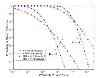
Figure 1: Complementary ROC curves for access point (AP) RIS configuration and RIS-relay configuration.

When the PU employs a RIS access point, then from (4), (12), (19) and (21), we obtain the total throughput as

$$T_{\textrm{ap}} =\lambda R_{s}\left\{\alpha P_{m}^{\textrm{ap}}+\left(1-\alpha\right)\left(1-P_{f}\right)\right\}$$

$$=\lambda R_{s}\left\{\alpha\textrm{erf}\left(\frac{\frac{y_{\textrm{th}}}{\bar{\gamma}r_{c}^{-\beta}}-N\left(\frac{\pi}{2}\right)^{\frac{1}{2}}}{\sqrt{2N\left(2-\frac{\pi}{2}\right)}}\right)\right.$$

$$\qquad\qquad\qquad\qquad\left.+\left(1-\alpha\right)\textrm{erf$\left(\sqrt{\frac{y_{\textrm{th}}}{2N_{0}}}\right)$}\right\},$$ (22)

where we have used the fact that $\textrm{erf}\left(x\right)=1-\textrm{erfc}\left(x\right)$ [20, Eq. (8.250.4)].

Similarly, when the CR node receives a PU transmission via a reflected RIS signal, then from (4), (18), (19) and (21), we obtain the total throughput as

$$T_{\textrm{rel}} =\lambda R_{s}\left\{\alpha P_{m}^{\textrm{rel}}+\left(1-\alpha\right)\left(1-P_{f}\right)\right\}$$

$$=\lambda R_{s}\left\{\alpha\textrm{erf}\left(\frac{\frac{y_{\textrm{th}}}{\bar{\gamma}\left(r_{c}r_{r}\right)^{-\beta}}-N\frac{\pi}{2}}{\sqrt{2N\left(4-\frac{\pi^{2}}{4}\right)}}\right)\right.$$

$$\qquad\qquad\qquad\qquad\left.+\left(1-\alpha\right)\textrm{erf$\left(\sqrt{\frac{y_{\textrm{th}}}{2N_{0}}}\right)$}\right\},$$ (23)

It is worth noting that given that for the RIS configurations, where the SNR becomes maximized, then as $N\rightarrow\infty,$ the detection threshold $y_{\textrm{th}}$ becomes very large, such that the second error function (in (22) and (23)) becomes $\lim{}_{\begin{subarray}{c}x\rightarrow\infty\end{subarray}}\textrm{erf}\left(x\right)=1$. It can therefore be shown that the asymptotic throughput of the CR node for the RIS access point configuration and the RIS relay configuration are respectively given by

$$T_{\textrm{ap}}^{\textrm{asym}} =\lambda R_{s}\left\{1-\alpha+\alpha\textrm{erf}\left(\frac{\frac{y_{\textrm{th}}}{\bar{\gamma}r_{c}^{-\beta}}-N\left(\frac{\pi}{2}\right)^{\frac{1}{2}}}{\sqrt{2N\left(2-\frac{\pi}{2}\right)}}\right)\right\}$$ (24)

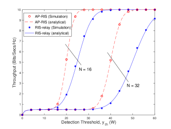
Figure 2: Throughput against detection threshold for both access point (AP) RIS configuration and RIS-relay configuration, showing different number of RIS cells $N$.

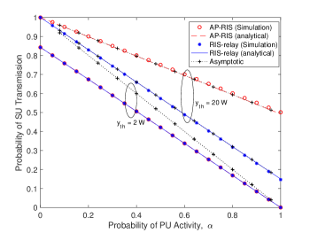
Figure 3: Probability of SU transmission against Probability of PU activity $\alpha$ for both access point RIS configuration and RIS-relay configuration. The asymptotic expressions are also indicated for different detection thresholds. RIS Cells $N=16.$

$$T_{\textrm{rel}}^{\textrm{asym}} =\lambda R_{s}\left\{1-\alpha+\alpha\textrm{erf}\left(\frac{\frac{y_{\textrm{th}}}{\bar{\gamma}\left(r_{c}r_{r}\right)^{-\beta}}-N\frac{\pi}{2}}{\sqrt{2N\left(4-\frac{\pi^{2}}{4}\right)}}\right)\right\}.$$ (25)

IV Numerical Results and Discussions

In this section, we present and discuss some results from the mathematical expressions derived in the paper. We then investigate the effect of key parameters on the system. The results are then verified using Monte Carlo simulations with at least $10^{5}$ iterations. Unless otherwise stated, we have assumed SNR $\bar{\gamma}=0$dB, PU activeness factor $\alpha=0.95$, $R_{s}=10$bits/secs/Hz, density $\lambda=1$ user/$m^{2}$ and all distances PU-to-RIS and RIS-to-CR normalized to unity. One benefit of normalizing the distances is to enable a direct comparison between the two configurations, as will be seen.

In Fig. 1, we plot the complementary receiver operating characteristics curve for both access point RIS and RIS-relay configurations. The analytical curves for $P_{f}$, $P_{m}^{\textrm{ap}}$ and $P_{m}^{\textrm{rel}}$, were plotted using the expressions from (4), (12) and (18), respectively, where $P_{m}=1-P_{d}$. We first note that the larger number of RIS cells in both configuration results in a better performance. In fact, it is possible to observe up to 3 to 4 orders of magnitude performance gain, when $N$ is doubled. Furthermore, it can be observed that the RIS-relay configuration performance better only up to about $10^{-3}$ point for the missed-detection range, while the AP-RIS performance better afterwards.

In Fig. 2, we present SU throughput results for both access point RIS and RIS-relay configurations. The analytical results for $T_{\textrm{ap}}$ and $T_{\textrm{rel}}$, were plotted from (22) and (23), respectively. Again we observe that increasing the number of RIS cells improves the throughput at any given detection threshold. Additionally, the results indicate that the RIS-relay configuration outperforms the access point RIS configuration. It is however worth noting that, an increased detection threshold, only indicates that the CR sensing node is willing to accept higher interference risk to the PU network, since a higher threshold means a higher likelihood of false alarm errors.

Next, in Fig. 3, we present a plot for the probability of SU transmission $P_{t}$ against the probability of PU activity $\alpha$ for both access point RIS and RIS-relay configurations ($N=16)$, as well as different detection threshold values. The asymptotic expressions for access point RIS and RIS-relay configurations, were plotted from (24) and (25), respectively, by assuming $\lambda=1$ and $R_{s}=1$. Here we observe that within the region of low detection threshold, where both RIS configurations provide similar SU transmission probabilities, the asymptotic expressions converge to the exact expressions, when PU activity is higher. On the other hand, when the detection threshold is higher, it can easily be observed that the asymptotic expressions converge to the exact expressions, even for very low PU activities. It can therefore be concluded that, due to the maximized SNR, only one hypothesis i.e. $H_{1}$ is enough for the SU to make a determination to transmit, while using both RIS configurations. It is also worth mentioning that, for a threshold as low as $y_{\textrm{th}}=5$W, the asymptotic and exact expressions converge. This has however been omitted in Fig. 3, to improve clarity of the curves.

V Conclusions

In this paper, we examined two popular configurations of RIS deployment as could be applied to a CR network. We derived expressions for the false alarm and detection probabilities as well as exact and asymptotic expressions for the SU transmission probability and throughput of the system. The results indicate how the use of RIS configurations by the PU can improve the task of spectrum sensing for the secondary CR and thereby improve the CR network performance. Further insights were obtained by observing the asymptotic case, where it was demonstrated that the CR could determine a transmission opportunity with a single hypothesis, due to the maximized SNR and higher detection thresholds allowed in the system.

References

- [1] M. D. Renzo, M. Debbah, D.-T. Phan-Huy, A. Zappone, M.-S. Alouini, C. Yuen, V. Sciancalepore, G. C. Alexandropoulos, J. Hoydis, H. Gacanin, J. d. Rosny, A. Bounceur, G. Lerosey, and M. Fink, “Smart radio environments empowered by reconfigurable AI meta-surfaces: An idea whose time has come,” EURASIP J. Wireless Commun. Netw., vol. 2019, no. 1, p. 129, May 2019. [Online]. Available: https://doi.org/10.1186/s13638-019-1438-9
- [2] C. Liaskos, S. Nie, A. Tsioliaridou, A. Pitsillides, S. Ioannidis, and I. Akyildiz, “A new wireless communication paradigm through software-controlled metasurfaces,” IEEE Commun. Mag., vol. 56, no. 9, pp. 162–169, Sep. 2018.
- [3] E. Basar, M. D. Renzo, J. D. Rosny, M. Debbah, M.-S. Alouini, and R. Zhang, “Wireless communications through reconfigurable intelligent surfaces,” IEEE Access, vol. 7, pp. 116 753–116 773, 2019.
- [4] E. Basar, “Transmission Through Large Intelligent Surfaces: A New Frontier in Wireless Communications,” in 2019 European Conf. Netw. Commun. (EuCNC), Jun. 2019, pp. 112–117.
- [5] S. Gong, X. Lu, D. T. Hoang, D. Niyato, L. Shu, D. I. Kim, and Y.-C. Liang, “Towards smart radio environment for wireless communications via intelligent reflecting surfaces: A comprehensive survey,” arXiv:1912.07794, Dec. 2019. [online]. Available: https://arxiv.org/abs/1912.07794.
- [6] A. U. Makarfi, K. M. Rabie, O. Kaiwartya, X. Li, and R. Kharel, “Physical Layer Security in Vehicular Networks with Reconfigurable Intelligent Surfaces,” in accepted for IEEE Veh. Technol. Conf. (VTC), Spring 2020, pp. 1–6.
- [7] H.-T. Chen, A. J. Taylor, and N. Yu, “A review of metasurfaces: physics and applications,” Reports on Progress in Physics, vol. 79, no. 7, p. 076401, Jun 2016. [Online]. Available: http://dx.doi.org/10.1088/0034-4885/79/7/076401
- [8] C. L. Holloway, E. F. Kuester, J. A. Gordon, J. O’Hara, J. Booth, and D. R. Smith, “An overview of the theory and applications of metasurfaces: The two-dimensional equivalents of metamaterials,” IEEE Ant. Propag. Mag., vol. 54, no. 2, pp. 10–35, Apr. 2012.
- [9] C. Huang, G. C. Alexandropoulos, A. Zappone, M. Debbah, and C. Yuen, “Energy efficient multi-user MISO communication using low resolution large intelligent surfaces,” in IEEE Global Commun. Conf. Workshops (GC Wkshps), Dec. 2018, pp. 1–6.
- [10] C. Huang, A. Zappone, G. C. Alexandropoulos, M. Debbah, and C. Yuen, “Reconfigurable intelligent surfaces for energy efficiency in wireless communication,” IEEE Trans. Wireless Commun., vol. 18, pp. 4157–4170, 2018.
- [11] L. Subrt and P. Pechac, “Controlling propagation environments using intelligent walls,” in 6th European Conf. Antennas Propag. (EUCAP), Mar. 2012, pp. 1–5.
- [12] Y. Liu, L. Zhang, B. Yang, W. Guo, and M. A. Imran, “Programmable wireless channel for multi-user MIMO transmission using meta-surface,” in IEEE Global Commun. Conf. (GLOBECOM), Dec 2019, pp. 1– 6.
- [13] C. Huang, A. Zappone, M. Debbah, and C. Yuen, “Achievable Rate Maximization by Passive Intelligent Mirrors,” in IEEE Int. Conf. Acoust. Speech Sig. Process. (ICASSP), Apr. 2018, pp. 3714–3718.
- [14] R. Zhang, Y. Liang, and S. Cui, “Dynamic Resource Allocation in Cognitive Radio Networks,” IEEE Sig. Process. Mag., vol. 27, no. 3, pp. 102–114, 2010.
- [15] D. Xu, X. Yu, Y. Sun, D. W. K. Ng, and R. Schober, “Resource Allocation for IRS-assisted Full-Duplex Cognitive Radio Systems,” arXiv:2003.07467v1, Mar. 2020. [online]. Available: https://arxiv.org/abs/2003.07467v1.
- [16] X. Guan, Q. Wu, and R. Zhang, “Joint Power Control and Passive Beamforming in IRS-Assisted Spectrum Sharing,” arXiv:2003.03105, Mar. 2020. [online]. Available: https://arxiv.org/abs/2003.03105.
- [17] J. Yuan, Y.-C. Liang, J. Joung, G. Feng, and E. G. Larsson, “Intelligent Reflecting Surface-Assisted Cognitive Radio System,” arXiv:1912.10678v1, Dec. 2019. [online]. Available: https://arxiv.org/abs/1912.10678v1.
- [18] L. Zhang, C. Pan, Y. Wang, H. Ren, K. Wang, and A. Nallanathan, “Robust Beamforming Design for Intelligent Reflecting Surface Aided Cognitive Radio Systems with Imperfect Cascaded CSI,” arXiv:2004.04595, Apr. 2020. [online]. Available: https://arxiv.org/abs/2004.04595v1.
- [19] A. U. Makarfi, K. M. Rabie, O. Kaiwartya, O. S. Badarneh, X. Li, and R. Kharel, “Reconfigurable Intelligent Surfaces-Enabled Internet-of-Things Networks in Generalized Fading Channels,” in accepted for IEEE Int. Conf. Commun. (ICC), Jun. 2020, pp. 1–6.
- [20] I. S. Gradshteyn and I. M. Ryzhik, Table of Integrals, Series, and Products. Califonia: Academic Press, 7th ed., 2007.
- [21] M. Abramowitz and I. A. Stegun, Handbook of Mathematical Functions with Formulas, Graphs, and Mathematical Tables, ninth dover printing, tenth gpo printing ed. New York: Dover, 1964.