On strongly rigid hyperfluctuating random measures
Abstract
In contrast to previous belief, we provide examples of stationary ergodic random measures that are both hyperfluctuating and strongly rigid. Therefore, we study hyperplane intersection processes (HIPs) that are formed by the vertices of Poisson hyperplane tessellations. These HIPs are known to be hyperfluctuating, that is, the variance of the number of points in a bounded observation window grows faster than the size of the window. Here we show that the HIPs exhibit a particularly strong rigidity property. For any bounded Borel set , an exponentially small (bounded) stopping set suffices to reconstruct the position of all points in and, in fact, all hyperplanes intersecting . Therefore, also the random measures supported by the hyperplane intersections of arbitrary (but fixed) dimension, are hyperfluctuating. Our examples aid the search for relations between correlations, density fluctuations, and rigidity properties.
Keywords: Strong rigidity, hyperfluctuation, hyperuniformity,
Poisson hyperplane
tessellations, hyperplane intersection processes
AMS MSC 2010: 60G55, 60G57, 60D05
1 Introduction
Let be a random measure on the -dimensional Euclidean space ; see [10, 14]. In this note all random objects are defined over a fixed probability space with associated expectation operator . Assume that is stationary, that is distributionally invariant under translations. Assume also that is locally square integrable, that is for all compact . Take a convex body , that is a compact and convex subset of and assume that has positive volume . In many cases of interest one can define an asymptotic variance by the limit
| (1.1) |
where the cases and are allowed. This limit may depend on ; but we do not include this dependence into our notation. Quite often the asymptotic variance is positive and finite. If, however, , then is said to be hyperuniform [19, 20]. If , then is said to be hyperfluctuating [20]. In recent years hyperuniform random measures (in particular point processes) have attracted a great deal of attention. The local behavior of such processes can very much resemble that of a weakly correlated point process. Only on a global scale a regular geometric pattern might become visible. Large-scale density fluctuations remain anomalously suppressed similar to a lattice; see [19, 20, 5]. The concept of hyperuniformity connects a broad range of areas of research (in physics) [20], including unique effective properties of heterogeneous materials, Coulomb systems, avian photoreceptor cells, self-organization, and isotropic photonic band gaps.
A point process on is said to be number rigid if the number of points inside a given compact set is almost surely determined by the configuration of points outside [16, 2]. Examples of number rigid point processes include lattices independently perturbed by bounded random variables, Gibbs processes with certain long-range interactions [3], zeros of Gaussian entire functions [8], stable matchings from [11], and some determinantal processes with a projection kernel [4].
It was proved in [6] that in one and two dimensions a hyperuniform point process is number rigid, provided that the truncated pair-correlation function is decaying sufficiently fast. Quite remarkably, it was shown in [16] that in three and higher dimensions a Gaussian independent perturbation of a lattice (which is hyperuniform) is number rigid below a critical value of the variance but not number rigid above. It is believed [5] that a stationary number rigid point process is hyperuniform. In this note we show that this is not true. In fact we give examples of stationary and ergodic (in fact mixing) random measures that are both hyperfluctuating and rigid in a very strong sense. The authors are not aware of any previously known rigid and ergodic process that is non-hyperuniform in dimensions (if is the unit ball). An example for has very recently been given in [12]. In this paper we will prove that the point process resulting from intersecting Poisson hyperplanes has very strong rigidity properties. This point process is hyperfluctuating [9] and, under an additional assumption on the directional distribution, mixing; see [18, Theorem 10.5.3] and Remark 2.1.
2 Poisson hyperplane processes
In this section we collect a few basic properties of Poisson hyperplane processes and the associated intersection processes. Let denote the space of all hyperplanes in . Any such hyperplane is of the form
| (2.1) |
where is an element of the unit sphere , and denotes the Euclidean scalar product. (Any hyperplane has two representations of this type.) We can make a measurable space by introducing the smallest -field containing for each compact the set
| (2.2) |
In fact, can be shown to be a closed subset of the space of all closed subsets of , equipped with the Fell topology. We refer to [18] for more details on this topology and related measurability issues; see also [14, Appendix A3].
We consider a (stationary) Poisson hyperplane process, that is a Poisson process on whose intensity measure is given by
| (2.3) |
where is an intensity parameter and (the directional distribution of ) is an even probability measure on . We assume that is not concentrated on a great subsphere. It would be helpful (even though not strictly necessary) if the reader is familiar with basic point process and random measure terminology; see e.g. [14]. For our purposes it is mostly enough to interpret as a random discrete subset of . The number of points (hyperplanes) in a measurable set is then given by and has a Poisson distribution with parameter . Since is invariant under translations (we have for all that ), the Poisson process is stationary, that is distributionally invariant under translations. Furthermore we can derive from Campbell’s theorem (see e.g. [14, Proposition 2.7]) and (2.3) that
| (2.4) |
As usual we assume (without loss of generality) that for all and all compact . More details on Poisson hyperplane processes can be found in [18, Section 4.4].
Let . We define a random measure on by
| (2.5) |
for Borel sets , where denotes summation over pairwise distinct entries and where is the Hausdorff measure of dimension ; see e.g. [14, Appendix A.3]. Using the arguments on p. 130 of [18] one can show that almost surely for all distinct the intersection is either empty or has dimension . Combining this with (2.4), we see that the random measures are almost surely locally finite, that is finite on bounded Borel sets. The random variable is the volume contents (in the appropriate dimension) of all possible intersections of hyperplanes within .
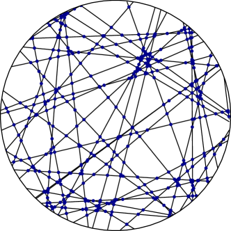
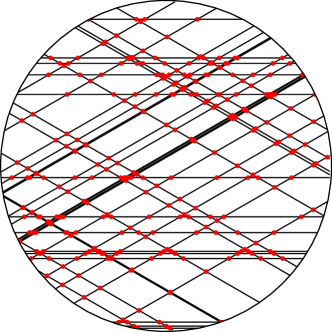
It can be shown that (almost surely) the intersection of different hyperplanes from is empty. Therefore the random measure is almost surely a point process without multiplicities, so that is just the number of (intersection) points with for some . It is convenient to define a simple (and locally finite) point process as the set of all points with for some . When (as it is common) interpreting as a random counting measure, we have that . Figure 1 shows two samples of and .
Among other things, Theorem 4.4.8 in [18] gives a formula for the intensity of . We only need to know that it is positive and finite. In the remaining part of this section we recall some second order properties of . (At first reading some details could be skipped without too much loss.) Let be bounded Borel subsets of . Using the theory of U-statistics [14, Section 12.3] it was shown in [13] that
| (2.6) |
where
| (2.7) |
If , this has to be read as
The asymptotic variance was derived in [9]. We note that is finite (this is implied by the form (2.3) of ) and that iff
Since is not concentrated on a great subsphere, this happens if and only if the Lebesgue measure of vanishes; see the proof of [18, Theorem 4.4.8]. Therefore we obtain from (2.6) that the random measures are hyperfluctuating (if ). The results in [9, 13] show that, for each finite collection of bounded Borel sets, the random vector converges in distribution to a multivariate normal distribution.
It is worth noting that the asymptotic covariances (2) are non-negative. If is isotropic (meaning that is the uniform distribution on ), there exist more detailed non-asymptotic second order results. In this case [9, p. 936] shows the pair correlation function (see e.g. [14, Section 8.2]) of the intersection point process is given by
| (2.8) |
where the coefficients are strictly poisitive and do only depend on the dimension. Hence, as , only at speed . In particular, the truncated pair correlation function is not integrable outside of any neighborhood of the origin. Using the well-known formula [14, Exercise 8.9]
(valid for all bounded Borel sets ) and assuming that is convex, it is not too hard to confirm (2.6) (using polar coordinates) for and a certain positive constant . The value of this constant can be found in [9].
Remark 2.1.
Assume that vanishes on any great subsphere. Then the random measures have the following mixing property. Let . Then can be interpreted as a random element in a suitably space of measures on equipped with a suitable -field [10, 14]. Let be arbitrary measurable subsets of . Then
where the random measure is defined by for Borel sets . This is a straightforward consequence of [18, Theorem 10.5.3] and the fact that is derived from in a translation invariant way. In particular is ergodic, that is for each translation invariant measurable set .
3 A reconstruction algorithm
Let be a Poisson hyperplane process as in Section 2. Let be the intersection point process associated with . (Recall from Section 2 that , where is given by (2.5) for .) Let be a non-empty convex and compact set. In this section we describe an algorithm which reconstructs (see Algorithm 3.3 and Fig. 2) by observing the points of in a (random) bounded domain in the complement of . In the next section we shall show that this domain is exponentially small.
We say that points from are in general hyperplane position if any of them are affinely independent and span the same hyperplane. The straightforward idea of the algorithm comes from the following proposition of some independent interest. We have not been able to find this result in the literature.
Proposition 3.1.
Almost surely the following is true. Any distinct points in general hyperplane position span a hyperplane .
Proof.
We start the proof with an auxiliary observation. Let and let be a measurable function on taking values in the space of all non-empty closed subsets of . (We equip this space with the usual Fell–Matheron topology; see [18]). We assert that
| (3.1) |
Obviously the indicator function of the event in (3.1) can be bounded by
If , then (3.1) follows. By the multivariate Mecke formula [14, Theorem 4.5],
By Fubini’s theorem it then enough to prove that
| (3.2) |
for any non-empty closed set . By monotonicity of integration it is sufficient to assume that for some . But then (3.2) directly follows from (2.3) and for each .
We now turn to the main part of the proof. Let be distinct with . We shall refer to these sets as blocks and to subsets of blocks as subblocks. For convenience we assume that . Assume that for some . Consider with for and the following properties. For each we have that consists of a single point and are in general hyperplane position. Let be affine hull of . We will show that almost surely .
Let us assume on the contrary that . Then each (for instance ) belongs to at most of the blocks. Indeed, by the general hyperplane assumption we would otherwise have that . We will show that almost surely
| (3.3) |
for all subblocks .
We prove (3.3) by (descending) induction on the cardinality of . In the case (3.3) holds by definition of . So assume that (3.3) holds for all subblocks of cardinality . We need to show that it holds for each subblock of cardinality . For notational convenience we take . By induction hypothesis we have that
| (3.4) |
Set . Since we have (almost surely) that . Since we therefore obtain that . Let us first assume that . By (3.4) (and since ) we have that . Therefore we obtain that , that is . Since is contained in at most of the subblocks, for instance in , the blocks still generate , that is . Therefore is “independent” of , contradicting . More rigorously we can apply (3.1) to conclude that this case can almost surely not occur. Let us now assume that . Then and therefore . This means that , as required to finish the induction.
Using (3.4) for subblocks of size , yields that for each . This contradiction finishes the proof of the lemma. ∎
Remark 3.2.
In general it is not possible to reduce the number of points featuring in Proposition 3.1. To see this, we may consider the case and a directional distribution which is concentrated on , where is an orthonormal system. In that case there exist infinitely many choices of four intersection points in general hyperplane position whose affine hull is not a hyperplane from . Indeed, the hyperplanes tessellate space into cuboids and the four points can be chosen as endpoints of diametrically oposed edges of any cuboid.
Our algorithm requires some notation. Let
denote the Euclidean distance between and and let
| (3.5) |
denote the outer parallel set of at distance . Note that . Define random times , , inductively by setting
where . We form a (random) set of hyperplanes as follows. A hyperplane belongs to if it does not intersect and if it contains different points from in general hyperplane position. By Proposition 3.1 we have almost surely that . For a hyperplane with we let denote the half-space bounded by with .
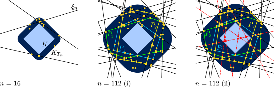
Algorithm 3.3.
The algorithm iterates over the random times , , (recursively) scanning the points in . If the algorithm stops at time , then it returns a set of hyperplanes that will be proved to coincide (almost surely) with . Stage of the algorithm is defined as follows (cf. Fig. 2):
-
(i)
Determine and check whether there are integers and distinct (, ) such that the boundary of
is contained in for each . If such hyperplanes do not exist, the algorithm continues with stage . If they do exist, the algorithm continues with step (ii) and stops after it.
-
(ii)
Find all collections of points in in general hyperplane position such that the generated hyperplane intersects . If there are such points, is the set of all those hyperplanes. If there are no such points, then .
Let if the algorithm stops at stage . We set if it never stops. We can interpret as the running time of the algorithm in continuous time. In the next section we will not only show that is (almost surely) finite but does also have exponential moments. Here we wish to assure ourselves of the essentially geometric fact that the algorithm indeed determines .
Proposition 3.4.
On the event we have almost surely that .
Proof.
Assume that the algorithm stops at at stage and let be as in step (i) of the algorithm. These are bounded polytopes which contain in their interior and which are made up of different hyperplanes from . Assume that intersects . Then intersects for each the boundary of the polytope , and in fact, at least one of its edges. Therefore there exist distinct hyperplanes such that
where . Almost surely each of these intersections consists of only one point , say. We assert that these points are in general hyperplane position. If they are not, then among those points, say, are affinely dependent. Then one of those points, say, must lie in . Therefore we need to show that the probability of finding distinct such that is a singleton for each and
is zero. Similarly as in the proof of (3.1) this probability can be bounded by
Therefore it is enough to show that for -a.e. and each affine space of dimension at most
| (3.6) |
where is the measure on the space of all affine subspaces of given by
For -a.e. , the measure is concentrated on the -dimensional subspaces of and invariant under translations in . In fact, is the intensity measure of the Poisson process . Up to a constant multiple,
is (as a function of the Borel set ) the intensity measure of the intersection process associated with (see [18, p. 135]) and therefore proportional to Lebesgue measure on . (It can also be checked more directly, that this function is a locally finite translation invariant measure.) Hence (3.6) follows. ∎
Remark 3.5.
Assume that that the directional distribution is absolutely continuous with respect to Lebesgue measure on . Then the algorithm can be considerably simplified. In step (i) it is enough two find just two polytopes made up of distinct hyperplanes in . Any hyperplane from that intersects , intersects the boundary of the polytope in affinely independent points from and the same applies to (even without further assumptions of ). With some efforts it can be shown that the resulting intersection points are almost surely in general hyperplane position. The forthcoming Theorem 4.1 remains valid. We do not go into the technical details.
Remark 3.6.
The reconstruction algorithm 3.3 is not optimized for computational efficiency. For instance, the algorithm could already be stopped whenever there exists just one polytope which contains in its interior but no points of in the relative interior of its edges. (In this case .) Moreover, it is not necessary that the boundaries of the polytopes are completely contained in . It would suffice to find polyhedral sets with sufficiently large parts of their boundaries contained in .
4 Strong rigidity
In this section we shall exploit the algorithm from Section 3 to show that the intersection processes associated with a Poisson hyperplane process have very strong rigidity properties.
We start with giving a few definitions. Let be a random measure on (for instance one of the ). For a Borel set we denote by the restriction of to . A mapping from into the space of non-empty closed subsets of is called -stopping set if is for each closed set an element of the -field generated by . (In particular is then a random closed set [15].) By we understand the restriction of to (that is the random measure .) If is a -stopping set, then we say that is almost surely determined by , if there exists a measurable mapping (with suitable domain) such that holds almost surely.
The following result shows that is almost surely determined by a -stopping set of exponentially small size. Here we quantify the size of a closed set by the radius of the smallest ball centred at the origin and containing . (If is not bounded then we set .)
Theorem 4.1.
Let be convex and compact. Then there exists a -stopping set with and such that is almost surely determined by . Moreover, there exist constants such that
| (4.1) |
Proof.
We consider the algorithm from Section 3 with running time , defined after Algorithm 3.3. We assert that has all desired properties, where . The inclusion is a direct consequence of the definitions. The stopping set property can be considered as pretty much obvious. The reader might wish to skip the following technical argument. Define as the set of all locally finite subsets of . The algorithm from Section 3 can be used (in an obvious way) to define a measurable mapping from (equipped with the standard -field) to the space of all closed subsets of such that . We need to show that is a stopping set, that is is for all closed sets an element of the -field generated by the mapping from to . To prove this we use [1, Proposition A.1]. According to this proposition it is sufficient to show that for all with . But this follows from the definition of the algorithm. Indeed, suppose that is a realization of the intersection process and that the algorithm stops at time . Restricting to and then adding a configuration in the complement of does not change the running time .
We show (4.1) by modifying the idea of the proof of Lemma 1 in [17]. Since is not concentrated on a great subsphere there exist linearly independent vectors in the support of . Since is even, the vectors are also in the support of . We can then find a (large) constant and (small) pairwise disjoint closed neighborhoods of , , such that and each intersection
with , , is a polytope with . Here we write, for given and , . Let . From linearity of the scalar product we then obtain that
| (4.2) |
whenever and for .
We need a straightforward analytic fact. Since the determinant is a continuous function we can assume that there exists such that
| (4.3) |
For let and . Then consists of a single point (by (4.3) and ), whose Euclidean norm can be bounded as
| (4.4) |
where is a constant that depends only on the dimension and the (fixed) sets . To see this we note that (now interpreted as a column vector) is the unique solution of the linear equation , where is the matrix with rows and is the column vector with entries . By (4.3) we have that . It is well-known that
where and is the maximum absolute row sum of . In view of the explicit expression of in terms of and the minors of and the minimum principle for continuous functions we have that is bounded from above by a positive constant. (Recall that are unit vectors.) Since for some we obtain (4.4).
For notational simplicity we now assume that is a ball with radius centred at the origin. In fact, in view of the assertion this is no restriction of generality. Consider the following sets of hyperplanes:
We assert the event inclusion
| (4.5) |
where with as in (4.4).
To show (4.5), we assume that for each . Then we can find distinct hyperplanes (, ) not intersecting such that the polytopes
contain in their interior and satisfy ; see (4.2). Next we show that each is in as soon as . (Then our algorithm has identified these hyperplanes by time .) Take , for instance. Define by . It can then be shown as in the proof of Proposition 3.4 that these points are in general hyperplane position. Therefore we obtain from (4.4) and the definition of that and in fact for each . Therefore , provided that . We have already seen that , so that the boundary of is contained in if . (Note that is a spherical shell with outer radius centred at the origin.) Altogether we obtain that and hence , proving (4.5).
Remark 4.2.
The stopping set in Theorem 4.1 depends measurably on (is a measurable function of ). This follows from the definition of the algorithm, but also from the following argument, which applies to general stopping sets with the property . By standard properties of random closed sets it suffices to check for each compact that . Since we have that . Since is compact, there is a decreasing sequence of open sets with intersection and such that
Since is a -stopping set we have that the above right-hand side is contained in , as asserted.
Theorem 4.1 implies the announced strong rigidity properties of the intersection processes.
Theorem 4.3.
Let and let be a bounded Borel set. Then there exists a -stopping set with and such that is almost surely determined by . Moreover, there exist constants such that (4.1) holds.
Proof.
Choose a convex and compact set with . Clearly, if the assertion holds in the case , then we obtain it for all . Hence we can assume that . Let be as in Theorem 4.1. Since is for each closed a measurable function of it follows that is a -stopping set. Moreover, is a (measurable) function of . Hence Theorem 4.1 implies the assertions. ∎
5 Hyperfluctuating Cox processes and thinnings
The strong rigidity property of the random measures can easily be destroyed by additional randomization. For example we may consider, for , a Cox process directed by [14, Chapter 13]. This means that the conditional distribution of given is that of a Poisson process with intensity measure . For this point process can be interpreted as a multiset (or a random measure). Each point of gets (independently of the other points) a random multiplicity having a Poisson distribution of mean 1. Let be a bounded Borel set. Then the well-known conditional variance formula (together with the stationarity of ) implies that
where is the intensity of ; see [14, Proposition 13.6]. By (2.6), has the same variance asymptotics as . In particular, is (for ) hyperfluctuating. However, is not rigid. For example, given a Borel set with positive volume, is not determined by the restriction of to the complement of .
In the case of the intersection point process there is an even simpler way of randomizing, namely to form a -thinning of for some . Formally, given , the points of are taken independently of each other as points of with probability [14, Section 5.3]. This point process is not rigid. A simple calculation (using the conditional variance formula for instance) shows that
so that inherits the variance asymptotics from . It also not hard to see that the pair correlation function of is the same as that of and hence given by the slowly decaying function (2.8).
6 Concluding remarks
We have shown that the intersection point process associated with a stationary Poisson hyperplane process is rigid in a very strong sense. This holds for any directional distribution which is not concentrated on a great subsphere. (Our arguments suggest that this might be true for more general stationary and mixing hyperplane processes with absolute continuous factorial moment measures.) On the other hand, is hyperfluctating. Hence hyperuniformity is not necessary for rigidity as (weakly) conjectured in [6]. However, we completely agree with the authors of [6] that the precise relationships between rigidity and hyperuniformity constitute an interesting intriguing problem. We believe in the existence of generic point process assumptions that need to be added to rigidity to conclude hyperuniformity. Preferably these assumptions should be as minimal as possible.
Acknowledgements: This research was supported in part by the Princeton University Innovation Fund for New Ideas in the Natural Sciences. The authors wish to thank Daniel Hug and Salvatore Torquato for valuable discussions of some aspects of our paper.
References
- [1] V. Baumstark and G. Last. Gamma distributions for stationary Poisson flat processes. Adv. in Appl. Probab. 41, 911-939, 2009.
- [2] A.I. Bufetov (2016). Rigidity of determinantal point processes with the Airy, the Bessel and the Gamma kernel. Bulletin of Mathematical Sciences 6.1, 163–172.
- [3] D. Dereudre, A. Hardy, T. Leblé, and M. Maïda (2018). DLR equations and rigidity for the Sine-beta process. arXiv:1809.03989.
- [4] S. Ghosh and M. Krishnapur (2015). Rigidity hierarchy in random point fields: random polynomials and determinantal processes. arXiv:1510.08814.
- [5] S. Ghosh and J.L. Lebowitz (2017). Fluctuations, large deviations and rigidity in hyperuniform systems: A brief survey. Indian J. Pure Appl. Math. 48, 609–631.
- [6] S. Ghosh and J.L. Lebowitz (2017). Number rigidity in superhomogeneous random point fields. J. Stat. Phys. 166, 1016–1027.
- [7] S. Ghosh and J.L. Lebowitz (2018). Generalized stealthy hyperuniform processes: Maximal rigidity and the bounded holes conjecture. Communications in Mathematical Physics 363(1), 97–110.
- [8] S. Ghosh and Y. Peres (2017). Rigidity and tolerance in point processes: Gaussian zeros and Ginibre eigenvalues. Duke Math. J. 166, 1789–1858.
- [9] L. Heinrich, H. Schmidt and V. Schmidt (2006). Central limit theorems for Poisson hyperplane tessellations. Ann. Appl. Probab. 16, 919–950.
- [10] O. Kallenberg (2002). Foundations of Modern Probability. Second Edition, Springer, New York.
- [11] M.A. Klatt, G. Last and D. Yogeshwaran (2018). Hyperuniform and rigid stable matchings. To appear in Random Structures & Algorithms.
- [12] R. Lachièze-Rey (2020). Variance linearity for real Gaussian zeros. arXiv:2006.10341.
- [13] G. Last, M.P. Penrose, M. Schulte and C. Thaele (2014). Moments and central limit theorems for some multivariate Poisson functionals. Adv. Appl. Probab. 46, 348–364.
- [14] G. Last and M. Penrose (2017). Lectures on the Poisson Process. Cambridge University Press.
- [15] I. Molchanov (2005). Theory of Random Sets. Springer, London.
- [16] Y. Peres and A. Sly (2014). Rigidity and tolerance for perturbed lattices. arXiv:1409.4490.
- [17] R. Schneider (2019). Interaction of Poisson hyperplane processes and convex bodies. J. Appl. Probab. 56, 1020–1032.
- [18] R. Schneider and W. Weil (2008). Stochastic and Integral Geometry. Springer, Berlin.
- [19] S. Torquato and F.H. Stillinger (2003). Local density fluctuations, hyperuniformity, and order metrics. Phys. Rev. E 68, 041–113.
- [20] S. Torquato (2018). Hyperuniform states of matter. Phys. Rep. 745, 1–95.