The Fairness-Accuracy Pareto Front

Abstract

Algorithmic fairness seeks to identify and correct sources of bias in machine learning algorithms. Confoundingly, ensuring fairness often comes at the cost of accuracy. We provide formal tools in this work for reconciling this fundamental tension in algorithm fairness. Specifically, we put to use the concept of Pareto optimality from multi-objective optimization and seek the fairness-accuracy Pareto front of a neural network classifier. We demonstrate that many existing algorithmic fairness methods are performing the so-called linear scalarization scheme which has severe limitations in recovering Pareto optimal solutions. We instead apply the Chebyshev scalarization scheme which is provably superior theoretically and no more computationally burdensome at recovering Pareto optimal solutions compared to the linear scheme.

1 Introduction

The emerging field of algorithmic fairness is concerned with the understanding and correcting of biases in machine learning algorithms. The scope of algorithmic fairness research is wide, including such goals as understanding post-hoc the cause of bias in both the data collection and the algorithm, correcting pre-hoc the data collection and algorithm design process to mitigate unfairness, defining measurements of fairness, and establishing regulatory guidelines to govern algorithm deployment. In this work, we highlight an underappreciated challenge to ascertaining algorithmic fairness – while we would like an algorithm to be both fair and accurate, these two objectives actually conflict with each other. As an extreme example, a completely randomized classifier is also a perfectly fair classifier by almost all measures of fairness; we would, however, be loathe to accept the low accuracy and arbitrariness of randomization. Thus, recognizing fairness and accuracy as competing objectives, we put to use the concept of Pareto optimality. Specifically, we apply tools from multi-objective optimization to find the fairness-accuracy Pareto front of a deep neural network classifier.

A typical multi-objective optimization problem is given by $\operatorname*{arg\,min}_{\theta}[J_{1}(\theta),\ldots,J_{k}(\theta)]^{T}$, where each $J_{i}$ is a loss function from some parameter space $\Theta$ to $\mathbb{R}$. The task is made difficult by the fact that it is rarely possible to find a $\theta^{*}$ such that all individual objectives are minimized simultaneously at $\theta^{*}$. In such circumstances, one can appeal to Pareto optimality, a well-established notion in optimization (Emmerich and Deutz, 2018) that is used often in engineering and economics. Pareto optimality is based on the following partial order: for $a,b\in\mathbb{R}^{p}$, we say $a\leq b$ if and only if every component of $a$ is less than or equal to the corresponding component of $b$. We say $\theta\in\Theta$ is Pareto optimal if and only if it is non-dominated, i.e. there does not exist any $\tilde{\theta}\in\Theta$ such that $(J_{1}(\tilde{\theta}),\ldots,J_{k}(\tilde{\theta}))\leq(J_{1}(\theta),\ldots,J_{k}(\theta))$ with at least one strict inequality. Similarly, we say $\theta$ is weakly Pareto optimal if there exists no other $\tilde{\theta}$ such that $J_{i}(\tilde{\theta})<J_{i}(\theta)$ for all $i=1,\ldots,k$. Note that while a Pareto optimal point is also weakly Pareto optimal, the converse is not true. The Pareto front is the set of all Pareto optimal points. Figure 1 displays a toy Pareto front for a bi-objective optimization problem.

Figure 1: This diagram illustrates the difference between weakly Pareto optimal and Pareto optimal points. All other points in the feasible region, represented by the polygon, are dominated points. The Pareto front itself, consisting of Pareto optimal points, is highlighted in solid red while the weakly Pareto optimal pints that are not Pareto optimal are highlighted in dashed red.

Almost all techniques for finding the Pareto front are based on scalarization, i.e., turning the vector objective into a scalar one by aggregating the individual objectives. A successful scalarization scheme should satisfy the following two desiderata.

1. The solutions to the scalarized objective are (weakly) Pareto optimal.

2. All Pareto optimal points are recoverable from the scalarization scheme.

Linear scalarization

The simplest scalarization scheme is the linear scalarization scheme (Emmerich and Deutz, 2018). Here the vector objective is replaced with a weighted sum, which we will call a linear scalarization problem (LSP),

$$\sum_{i=1}^{k}\lambda_{i}J_{i},\quad\lambda_{i}\in\mathbb{R}_{>0},\quad i=1,\ldots,k.$$ (1)

Sometimes the constraint, $\sum_{i=1}^{k}\lambda_{i}=1$, is imposed, but this is not in fact necessary, e.g., if the individual objectives are not normalized. The linear scalarization scheme satisfies desideratum D1. Specifically, no matter the weights $\lambda_{i}$ chosen, a solution of the linear scalarization problem is weakly Pareto optimal, see Proposition 8 in (Emmerich and Deutz, 2018). However, the linear scalarization scheme critically fails desideratum D2. In fact, it is only able to recover points on the convex hull of the Pareto front (Das and Dennis, 1997). In particular, when the Pareto front of interest is non-convex, the naive linear scalarization scheme may only find such $\theta$ that strongly favors one of the objectives (Emmerich and Deutz, 2018). We illustrate this phenomenon in Figure 2.

Despite the known drawbacks to the linear scalarization scheme for finding Pareto optimal points, almost all train-time algorithmic fairness methods, to be reviewed in the following section, ascribe to this approach. To see this, we note that many popular algorithmic fairness techniques minimize an objective of the form

$$\text{error}(\theta)+\lambda\times\text{unfairness}(\theta),$$

where $\theta$ is the model parameters to be learned. That is, they regularize the learning algorithm by employing the fairness criterion as a penalty term during training (Hardt et al., 2016; Joseph et al., 2016; Zafar et al., 2017a, b). It is easy to recognize this constrained optimization as the linear scalarization problem in Equation equation 1. Thus existing algorithmic-fairness methods can be expected to inherit all the limitations of the linear scalarization scheme in regards to finding Pareto optimal points.

Figure 2: Two hypothetical Pareto fronts are displayed: convex (left) and non-convex (right). The dashed lines represent different weight combinations in the LSP equation 1. Pareto optimality occurs only at the tangential points of the dashed lines. It is clearly that the LSP cannot recover Pareto optimal points that reside in the non-convex region of the Pareto front.

Proposal

In this work, we use instead the Chebyshev scalarization scheme (Section 3) to find the fairness-accuracy Pareto front of a deep neural network classifier. The Chebyshev scheme is no more computationally burdensome than the linear scheme while enjoying theoretically superior performance when the Pareto front is non-convex (as it may well be). The final deliverable is a set of neural networks spanning the fairness-accuracy space from the high-accuracy-low-fairness corner to the high-fairness-low-accuracy corner. This could then be consulted by an interested party, e.g. a relevant regulatory body, to decide on a particular classifier with the acceptable trade-off.

In recognition of the dominant role inhabited by deep learning in predictive tasks, our examples are limited to deep neural network classifiers. We should note however that nothing prevents the application of the proposed framework to classifiers besides neural networks, as long as the classifier is amenable to training by backpropagation. This includes models that are more familiar to the statistical audience such as logistic regression and support vector machine. In fact, logistic regression is simply a multi-layer perception with no hidden layers and thus a special case of the feedforward neural network we will work with.

2 Related work

Multi-objective optimization in machine learning and statistics

Multi-objective optimization techniques are gaining increasing traction in machine learning (Yaochu Jin and Sendhoff, 2008). Bayesian optimization (Zhang and Golovin, 2020) and reinforcement learning (Moffaert and Nowe, 2014) seem to have particularly embraced ideas from multi-objective optimization. The multiple-gradient descent algorithm, a common gradient-based multiobjective optimization technique, has been applied to kernel learning Li et al. (2014) and Bayesian optimization Shah and Ghahramani (2016). Though multiple-gradient descent in its original form does not scale up to the high dimensionality of the parameter space of a neural network, Sener and Koltun (2018) proposed a workaround that demonstrated good results on standard deep learning benchmarking datasets. Another work in this vein seeks to further articulate user preference for a specific tradeoff, by dividing a deep multi-task learning problem into different subproblems (Lin et al., 2019).

Algorithmic fairness

Let us now briefly review those works in algorithm fairness that are concerned with correcting the bias of machine learning algorithms. These methods are set apart according to the stage in which intervention is taken. The first class of methods attempts to remove bias from the input data itself. These methods rest on the premise that once proper preprocessing is accomplished, any classifier can be used to produce subsequently fair predictions (Kamiran and Calders, 2012; Feldman et al., 2015; Calmon et al., 2017; Johndrow and Lum, 2019). On the other hand, post-processing techniques directly operate on the classifier output and are, in principle, amenable to any classifier. The technique in Hardt et al. (2016) for instance seeks to learn a monotone transformation of the classifier output to enforce demographic parity or equalized odds, two standard definitions of fairness that we will review in Section 4.

The third type of algorithmic fairness methods directly intervenes during training. Generally speaking, these train-time methods add the fairness criterion as a regularization term to the main objective of minimizing predictive error (Calders and Verwer, 2010; Kamishima et al., 2011; Zafar et al., 2017a, b, c; Bechavod and Ligett, 2017; Agarwal et al., 2018; Narasimhan, 2018). While early works of this type (Berk et al., 2017; Zafar et al., 2017b; Bechavod and Ligett, 2017) focused on simple machine learning algorithms such as logistic regression, more recent work (Beutel et al., 2017; Wadsworth et al., 2018; Madras et al., 2018; Manisha and Gujar, 2018) can handle more complex models such as neural networks.

The proposed work also intervenes at train time. It appears to be the first in the algorithmic fairness literature to advocate for the important role that Pareto optimality should play, considering that fairness and accuracy are competing objectives of interest. Many methods do not consider the trade-off curve or when they do, they do not use proper techniques to recover Pareto optimal points in the fairness-accuracy space.

3 The fairness-accuracy Pareto front

In this section, we apply the Chebyshev scalarization scheme to estimate the fairness-accuracy Pareto front of a neural network binary classifier. Suppose the data consists of input variables ${\mathbf{x}}\in{\mathbb{X}}\subset\mathbb{R}^{p}$ standardized to mean zero and unit variance, binary response ${\mathbf{y}}\in{\mathbb{Y}}$ indicating class membership, and binary sensitive variable ${\mathbf{a}}$. Let all discrete variables be dummy encoded. A feedforward neural network is a repeated composition of affine transformation followed by nonlinear transformation. Let $m_{0}=p$ and define $w^{(l)}\in\mathbb{R}^{m_{l}\times m_{l-1}}$ and $b^{(l)}\in\mathbb{R}^{m_{l}},l=1,\ldots,L$ as the parameters in the $l$-th layer of a fully-connected feedforward neural network with $L$ layers. Consider the affine transformation $h^{(l)}:\mathbb{R}^{m_{l-1}}\to\mathbb{R}^{m_{l}}$ and nonlinear transformation $v^{(l)}$ given by

$$h^{(l)} =w^{(l)}v^{(l-1)}+b^{(l)},\quad l=1,\ldots,L$$

$$v^{(l)} =\sigma^{(l)}\circ h^{(l)},\quad l=1,\ldots,L$$

where $v^{(0)}=id$ is the identity function and $\sigma^{(l)}:\mathbb{R}^{m_{l}}\to\mathbb{R}^{m_{l}}$ is a nonlinear transformation (more frequently called the activation function) that acts component-wise.

The activation function in the final layer, $\sigma^{(L)}$, will be restricted to the sigmoid function, $(1+\exp(-x))^{-1}$, so that the classifier outputs scores between $0$ and $1$. We use the ReLU activation function, $max(0,x)$, in all other layers for our experiments. Let ${\mathbf{h}}^{(l)}_{i}$ be shorthand for the application of the function $h^{(l)}$ to input feature ${\mathbf{x}}_{i}$, i.e.

$${\mathbf{h}}^{(l)}_{i}=h^{(l)}({\mathbf{x}}_{i}).$$

Collecting all parameters $(w^{(l)},b^{(l)}),l=1,\ldots,L$ into the parameter vector $\theta$, let $f_{\theta}:{\mathbb{X}}\to[0,1]$ be a fully-connected feedforward neural network with parameter $\theta\in\Theta$ constructed as above, i.e., the neural network acts as $f_{\theta}(x)=v^{(L)}(x)$.

Let $P$ be the joint distribution of the data $({\mathbf{x}},{\mathbf{a}},{\mathbf{y}}).$ The accuracy of $f_{\theta}$ will be measured by its risk,

$$R(\theta)=\mathbb{E}_{P}\mathcal{L}(f_{\theta}({\mathbf{x}}),{\mathbf{y}}),$$

where $\mathcal{L}$ is a loss function. Since we are interested in binary classification, we will limit future discussion to the binary cross-entropy loss, $\mathcal{L}:[0,1]\times\{0,1\}\to\mathbb{R}$ given by

$$\mathcal{L}(\hat{p},y)=y\log\hat{p}+(1-y)\log(1-\hat{p}).$$

Next, let $U(\theta)$ be some population measure for the fairness of $f_{\theta}$. We shall take the convention that higher values of $U$ are undesirable, yielding algorithms that are more unfair. Since we wish for the learning algorithm $f_{\theta}$ to be both accurate and fair, we have the following vector objective function

$$\operatorname*{arg\,min}_{\theta}\begin{bmatrix}R(\theta)\\ U(\theta)\end{bmatrix}.$$ (2)

Chebyshev scalarization

As an alternative to the linear scalarization scheme in equation 1, we consider the Chebyshev scalarization scheme (Ehrgott, 2000; Giagkiozis and Fleming, 2015) whereby the vector objective, $[J_{1}(\theta),\ldots,J_{k}(\theta)]^{T}$, is replaced with what we will call the Chebyshev scalarization problem (CSP),

$$\max_{i=1,\ldots,k}\{\lambda_{i}|J_{i}(\theta)-z_{i}^{*}|\},\quad\lambda_{i}\in\mathbb{R}_{>0},\quad i=1,\ldots,k$$ (3)

where $z_{i}^{*}=\inf_{\theta}J_{i}(\theta)$. The Chebyshev scalarization satisfies both desiderata D1 and D2. Namely the solutions to equation 3 are at least weakly Pareto optimal and hence possibly Pareto optimal but not necessarily. Furthermore, any Pareto optimal solution can be obtained for some configuration of $\lambda_{i}$’s, see Proposition 10 of (Emmerich and Deutz, 2018). In particular, this means the Chebyshev scheme can find Pareto optimal points that reside in the nonconvex area of the Pareto front in contrast to the linear scalarization scheme. Figure 3 contains an illustration of this. However, we caution that this does not mean that every CSP solution is Pareto optimal because again the solution may be weakly Pareto optimal.

More advanced scalarization schemes than either the LSP or the CSP certainly exist. However, we focus on the CSP in this paper as a first step in applying MOO to algorithmic fairness. CSP is an obvious candidate given its clear superiority to LSP. Furthermore there is no additional computational overhead to solve the CSP compared to the LSP.

Figure 3: We again consider the two hypothetical Pareto fronts from Figure 2. This time the dashed lines represent different weight combinations in the CSP equation 3. We can see that the CSP, in contrast to the LSP, can recover Pareto optimal points that reside in the non-convex region of the Pareto front.

Estimates of the individual components

Solving equation 3 first requires estimation of the population unknowns $R(\theta)$ and $U(\theta)$. Since most learning algorithms proceed by empirical risk minimization, we can without loss of generality estimate $R(\theta)$ with the plug-in estimator. Specifically let $R_{n}(\theta)=\mathbb{P}_{n}\mathcal{L}(f_{\theta}({\mathbf{x}}),{\mathbf{y}})$ where $\mathbb{P}_{n}=\frac{1}{n}\sum_{i=1}^{n}\delta_{({\mathbf{x}}_{i},{\mathbf{a}}_{i},{\mathbf{y}}_{i})}$ is the empirical measure for the training set $({\mathbf{x}}_{1},{\mathbf{a}}_{1},{\mathbf{y}}_{1}),\ldots,({\mathbf{x}}_{n},{\mathbf{a}}_{n},{\mathbf{y}}_{n})\sim P$. We will defer discussion of the estimation of $U(\theta)$ to Section 4 in the context of specific fairness metrics. For now, let $U_{n}(\theta)$ denote some estimator of $U(\theta)$ based on the dataset of sample size $n$. (It does not need to be the plug-in estimator.)

Standardization

The individual estimators $R_{n}$ and $U_{n}$ should be properly scaled so that the weights in equation 3 can better articulate user preferences. We will focus on discussing the standardization of $R_{n}$ and $U_{n}$ in the context where $f_{\theta}$ is a neural network. As mini-batches are almost always employed during training of a neural network, the risk and unfairness measures will be evaluated on mini-batches. Let $\{({\mathbf{x}}_{1}^{*},{\mathbf{a}}_{1}^{*},{\mathbf{y}}_{1}^{*}),\ldots,({\mathbf{x}}_{b}^{*},{\mathbf{a}}_{b}^{*},{\mathbf{y}}_{b}^{*})\}$ be a mini-batch sample drawn without replacement from $\mathbb{P}_{n}$. Then define the mini-batch estimate of the risk as $R_{b}^{*}(\theta)=\frac{1}{b}\sum_{i=1}^{b}\mathcal{L}(f_{\theta}({\mathbf{x}}_{i}^{*}),{\mathbf{y}}_{i}^{*}).$ Similarly, let $U_{b}^{*}(\theta)$ be the mini-batch estimate of the fairness measure.

First we solve equation 3 for $\lambda=0$. This will not typically be an exact solution. For instance if $f_{\theta}$ is a neural network, equation 3 can only be solved approximately, e.g. optimization via stochastic gradient descent. Let $R_{min}$ and $R_{max}$ denote, respectively, the minimum and maximum value of $R_{b}^{*}$ observed across the mini-batches over all epochs. We can similarly obtain $U_{min}$ and $U_{max}$ by solving equation 3 for $\lambda=1$. Then we standardize the accuracy and fairness components as follows

$$\tilde{R}_{n}(\theta)=(R_{n}(\theta)-R_{min})/(R_{max}-R_{min})$$

and

$$\tilde{U}_{n}(\theta)=(U_{n}(\theta)-U_{min})/(U_{max}-U_{min}).$$

Pareto front candidates

Using the Chebyshev scalarization scheme leads us to Pareto front candidates given by the set $\{\hat{\theta}_{n}^{\lambda}:\lambda\in\Lambda\}$ where

$$\hat{\theta}_{n}^{\lambda}=\operatorname*{arg\,min}_{\theta}\max\{(1-\lambda)\tilde{R}_{n}(\theta),\lambda\tilde{U}_{n}(\theta)\}.$$ (4)

and $\Lambda\subset[0,1]$ is a finite set of $\lambda$ values which includes $\lambda=0$ and $\lambda=1$. Note that equation 4 follows directly from equation 3 since the standardization step renders $z_{i}^{*}=0$ for all $i$. Ideally, we would then solve equation 4 for a dense $\Lambda$. While intuitive, evenly distributed $\lambda$’s in the interval $[0,1]$ should be avoided as this often produces solutions that form clumps in the Pareto front, i.e.  evenly distributed $\lambda$’s in $[0,1]$ do not produce evenly distributed points in the multi-objective space. The experiments in Section 5 employ approximately evenly-spaced values of $\lambda$ on the log scale for the set $\Lambda$. Future work might involve more sophisticated techniques from multi-objective optimization, e.g.  the Normal-Boundary-Interactive (Das and Dennis, 2000) which adaptively selects $\lambda$.

Algorithm 1 Fairness-accuracy Pareto front candidates

Input: multiple splits of the data into training set (sample size $n$) and testing set (sample size $T$), and a finite set $\Lambda\subset[0,1]$ which includes $\lambda=0$ and $\lambda=1$.

Initialize candidates $=\emptyset$.

for each training-testing split do

     Solve equation 4 on the training set to obtain $\hat{\theta}_{n}^{\lambda}$ for each $\lambda\in\Lambda$

     Add to candidates the set $\{\hat{\theta}_{n}^{\lambda}:\lambda\in\Lambda\}$

end for

Output: candidates

Finally, to get a robust estimate of the Pareto front, we should average out, so to speak, the randomness associated with the training-testing split. If $M$ pairs of training and testing splits are considered, then candidates, the output of Algorithm 1, contains in total $M|\Lambda|$ Pareto candidates.

Visualization of results

To visualize the estimated Pareto front, we plot each element of candidates, the output of Algorithm 1, in the fairness-accuracy space as evaluated on the test set. Specifically, we calculate the out-of-sample risk of $\theta$ as

$$R(\theta;\hat{P}_{\rm{test}}) =\mathbb{E}_{\hat{P}_{\rm{test}}}\mathcal{L}(f({\mathbf{x}};\theta),{\mathbf{y}})=\frac{1}{T}\sum_{i=1}^{T}\mathcal{L}(f({\mathbf{x}}_{i}^{*};\theta),{\mathbf{y}}_{i}^{*})$$

where $\hat{P}_{\rm{test}}=\frac{1}{T}\sum_{i=1}^{T}\delta_{({\mathbf{x}}_{i}^{*},{\mathbf{a}}_{i}^{*},{\mathbf{y}}_{i}^{*})}$ is the empirical measure of the test set $\{({\mathbf{x}}_{i}^{*},{\mathbf{a}}_{i}^{*},{\mathbf{y}}_{i}^{*})\}_{i=1}^{T}$ drawn independently from the (unknown) distribution $P$. Let $U(\theta;\hat{P}_{\rm{test}})$ denote the fairness metric assessed on the test set. Again it need not be a plug-in estimator. Each Pareto front candidate can then be visualized by plotting $R(\theta;\hat{P}_{\rm{test}})$ versus $U(\theta;\hat{P}_{\rm{test}})$ for every $\theta$ in candidates. We further cull these candidates by keeping only the non-dominated points, forming the final Pareto front estimate.

Each point on the estimated Pareto front corresponds to a different neural network classifier $f_{\theta}$. A practitioner can examine the estimated Pareto front to select the neural network with an acceptable trade-off between fairness and accuracy.

4 Fairness measures

We will be examining the fairness-accuracy Pareto front corresponding to a variety of fairness notions. In this section we begin by reviewing two common notions of fairness – demographic and conditional parity. We then review causal approaches to fairness. Along the way we introduce new estimators of conditional parity and introduce a new causal fairness measure, each of which may be of independent interest.

4.1 Demographic parity and conditional parity

Many standard fairness measures involve checking the statistical independence between the prediction and the sensitive attribute. The classifier $f_{\theta}({\mathbf{x}})$ is said to exhibit demographic parity with respect to the sensitive attribute ${\mathbf{a}}$ if $f_{\theta}({\mathbf{x}})\mathchoice{\mathrel{\hbox to0.0pt{$\displaystyle\perp$\hss}\mkern 2.0mu{\displaystyle\perp}}}{\mathrel{\hbox to0.0pt{$\textstyle\perp$\hss}\mkern 2.0mu{\textstyle\perp}}}{\mathrel{\hbox to0.0pt{$\scriptstyle\perp$\hss}\mkern 2.0mu{\scriptstyle\perp}}}{\mathrel{\hbox to0.0pt{$\scriptscriptstyle\perp$\hss}\mkern 2.0mu{\scriptscriptstyle\perp}}}{\mathbf{a}},$ where $\mathchoice{\mathrel{\hbox to0.0pt{$\displaystyle\perp$\hss}\mkern 2.0mu{\displaystyle\perp}}}{\mathrel{\hbox to0.0pt{$\textstyle\perp$\hss}\mkern 2.0mu{\textstyle\perp}}}{\mathrel{\hbox to0.0pt{$\scriptstyle\perp$\hss}\mkern 2.0mu{\scriptstyle\perp}}}{\mathrel{\hbox to0.0pt{$\scriptscriptstyle\perp$\hss}\mkern 2.0mu{\scriptscriptstyle\perp}}}$ stands for independence. Intuitively, demographic parity assesses whether the predicted score depends on the sensitive variable. For example, a classifier predicting if a convicted criminal will re-offend exhibits demographic parity with respect to race if the distribution of $f_{\theta}({\mathbf{x}})$ is the same irrespective of race. Despite its intuitiveness, the drawbacks to demographic parity are well-documented (Hardt et al., 2016; Kleinberg, 2018). For instance, when the base rates differ across values of the sensitive attribute, satisfying demographic parity can come at the cost of discrimination.

Conditional parity, a term coined in Ritov et al. (2017), is another notion of fairness that encompasses several fairness measures. The prediction $f_{\theta}({\mathbf{x}})$ is said to exhibit conditional parity with respect to sensitive attribute ${\mathbf{a}}$ conditioned on ${\mathbf{u}}$ if $f_{\theta}({\mathbf{x}})\mathchoice{\mathrel{\hbox to0.0pt{$\displaystyle\perp$\hss}\mkern 2.0mu{\displaystyle\perp}}}{\mathrel{\hbox to0.0pt{$\textstyle\perp$\hss}\mkern 2.0mu{\textstyle\perp}}}{\mathrel{\hbox to0.0pt{$\scriptstyle\perp$\hss}\mkern 2.0mu{\scriptstyle\perp}}}{\mathrel{\hbox to0.0pt{$\scriptscriptstyle\perp$\hss}\mkern 2.0mu{\scriptscriptstyle\perp}}}{\mathbf{a}}\mid{\mathbf{u}}.$ Conditional parity in fact unifies several existing fairness definitions. For instance, the notion of equalized odds, introduced in Hardt et al. (2016), is recovered by setting ${\mathbf{u}}$ to ${\mathbf{y}}$, the true target class membership itself.

That the notions of demographic and conditional parity can strongly differ and may lead to seemingly paradoxical results was strikingly illustrated in Bickel et al. (1975) for graduate admissions at UC Berkeley. Consider a classifier predicting whether an applicant should be admitted to graduate school. One may desire admission decisions to be independent of gender (demographic parity), or independent of gender conditional on a particular university department (conditional parity). Depending on which fairness measure is employed, radically different conclusions may be reached.

We propose to assess demographic and conditional parity using the mean-variance statistic proposed in Cui et al. (2015). The development of these estimators is not central to the proposed work but may be of separate interest so we defer its presentation to Appendix B.2.

4.2 Causal fairness in the overlap population

Taking the causal approach to defining fairness means replacing the question “Is the learning prediction (conditionally) dependent on the sensitive attribute?” with the question “Does the sensitive attribute have a causal effect on the learning predictions?” Causal approaches to defining fairness (Kusner et al., 2017; Kilbertus et al., 2017; Loftus et al., 2018; Khademi et al., 2019) are motivated by the consideration that selection bias will result in a study population different from the target population. This is precisely the situation in many datasets of interest in algorithmic fairness. For instance, in predicting recidivism, the training data suffers selection bias leading to a training population (re-offenders that were caught) likely different from the target population (all would-be re-offenders).

We propose a new causal fairness measure which assesses the average effect of ${\mathbf{a}}$ on the predicted probabilities $f_{\theta}({\mathbf{x}})$ in the so-called overlap population introduced in Li et al. (2018). The overlap population is of particular policy relevance. It is the subpopulation where the sensitive attribute ${\mathbf{a}}$ occurs with equal probability, given the prediction inputs ${\mathbf{x}}$. For instance, in the context of recidivism prediction, the overlap population is the subpopulation with similar inputs, e.g. criminal record, demographic characteristics, who could easily be either Caucasian or from a minority group. In contrast, many traditional causal estimands focus on unrealistic target populations comprised of individuals who are atypical for their particular value of ${\mathbf{a}}$.

Adopting the potential outcome framework of Imbens and Rubin (2015) and assuming the Stable Unit Treatment Value Assumption, suppose the outcome of interest ${\mathbf{o}}$ takes on one of two potential outcomes, either ${\mathbf{o}}(0)$ or ${\mathbf{o}}(1)$, depending on whether ${\mathbf{a}}=0$ or ${\mathbf{a}}=1$. Note that ${\mathbf{o}}={\mathbf{o}}(1){\mathbf{a}}+{\mathbf{o}}(0)(1-{\mathbf{a}})$, i.e. we can only ever observe one of the two potential outcomes. Furthermore, suppose the condition of unconfoundedness is satisfied, i.e. ${\mathbf{a}}$ is independent of $\{{\mathbf{o}}(0),{\mathbf{o}}(1)\}$ conditional on ${\mathbf{x}}$.

The average treatment effect for the overlap population (ATO) introduced in Li et al. (2018) is given by

$$\tau_{ATO}({\mathbf{o}};P)=\frac{\mathbb{E}_{P}[e({\mathbf{x}})(1-e({\mathbf{x}}))(\mathbb{E}({\mathbf{o}}(1)\mid{\mathbf{x}})-\mathbb{E}({\mathbf{o}}(0)\mid{\mathbf{x}}))]}{\mathbb{E}_{P}[e({\mathbf{x}})(1-e({\mathbf{x}}))]}$$

where $e(x)=\displaystyle P({\mathbf{a}}=1\mid{\mathbf{x}}=x)$ is also called the propensity score. Again, the term overlap refers to the fact that the ATO articulates the causal effect among the overlap population which consists of subjects, given their covariates, who could appear with substantial probability in either value of the sensitive attribute. Consider measuring fairness as the causal effect of ${\mathbf{a}}$ on the predicted probability $f_{\theta}({\mathbf{x}})$ in the overlap population, i.e.

$$U(\theta) =\left|\tau_{ATO}(f_{\theta}({\mathbf{x}});P)\right\rvert.$$

Its evaluation on the test set is straightforward. Define

$$U(\theta,\hat{P}_{\rm{test}})=\left|\tau_{ATO}(f_{\theta}({\mathbf{x}});\hat{P}_{\rm{test}})\right\rvert.$$

Estimation of the ATO causal estimand first requires estimating the propensity score. In our experiments, we used a neural network to do this. We then calibrated the predicted probabilities using the temperature scaling procedure of Guo et al. (2017). Further details follow in the experiments section. For now, let $\hat{e}(x)$ denote the propensity score estimate. Li et al. (2018) proposed estimating $\tau_{ATO}$ as follows:

$$\hat{\tau}_{ATO}({\mathbf{o}})=\frac{\sum_{i=1}^{n}{\mathbf{a}}_{i}{\mathbf{o}}_{i}w_{i}}{\sum_{i=1}^{n}{\mathbf{a}}_{i}w_{i}}-\frac{\sum_{i=1}^{n}(1-{\mathbf{a}}_{i}){\mathbf{o}}_{i}w_{i}}{\sum_{i=1}^{n}(1-{\mathbf{a}}_{i})w_{i}}$$ (5)

where $w_{i}$ are the so-called overlap weights given by

$$w_{i}=\begin{cases}1-\hat{e}({\mathbf{x}}_{i})&\text{if ${\mathbf{a}}_{i}=1$}\\ \hat{e}({\mathbf{x}}_{i})&\text{if ${\mathbf{a}}_{i}=0$.}\end{cases}$$ (6)

Notably, the overlap weights smoothly down-weigh subjects in the tails of the propensity score distribution, thereby mitigating the common problem of extreme propensity scores. In contrast, the standard inverse probability weights can suffer from excessive variance and correspond to emphasis on a target population which may consist of subjects very atypical for their particular value of ${\mathbf{a}}$.

In our experiments we considered two possibilities for $U_{n}(\theta)$. In the first, we measure the average effect in the overlap population of ${\mathbf{a}}$ on the penultimate layer of the neural network, ${\mathbf{h}}^{(L-1)}$ leading to

$$U_{n}(\theta)=\left|\hat{\tau}_{ATO}({\mathbf{h}}^{(L-1)})\right\rvert=\frac{\sum_{i=1}^{n}{\mathbf{a}}_{i}{\mathbf{h}}_{i}^{(L-1)}w_{i}}{\sum_{i=1}^{n}{\mathbf{a}}_{i}w_{i}}-\frac{\sum_{i=1}^{n}(1-{\mathbf{a}}_{i}){\mathbf{h}}_{i}^{(L-1)}w_{i}}{\sum_{i=1}^{n}(1-{\mathbf{a}}_{i})w_{i}}$$ (7)

where $w_{i}$ are the overlap weights as in equation 6. In the second option for $U_{n}$, we measure the average effect of ${\mathbf{a}}$ on all intermediate layers of the neural network, leading to

$$U_{n}(\theta)=\sum_{l=1}^{L-1}\left\lvert\hat{\tau}_{ATO}({\mathbf{h}}^{(l)})\right\rvert.$$ (8)

The benefits of learning fair internal representations in a neural network was recognized in Madras et al. (2018). In particular, we may expect doing so can safeguard against bias in further downstream analyses, such as transfer learning.

5 Experiments

We apply the proposed Pareto front estimation procedure to two benchmarking datasets in the algorithmic fairness literature: the ProPublica recidivism dataset and the UCI adult income dataset. The two datasets are summarized in Table 1. We also examine two possibilities for $U_{n}$ in Algorithm 1 corresponding to either equation 7 or equation 8, i.e., calculating the ATO in either the penultimate layer or all intermediate layers of the neural network respectively.

Table 1: Dataset descriptions

	dataset features
Dataset	$dim({\mathbf{x}})$	binary outcome $y$	sensitive ${\mathbf{a}}$	training size	testing size	minibatch size
Recidivism	12	Re-offend in 2 years?	binary race	3086	3086	150
UCI	93	Income above 50K?	binary race	15470	15470	1000
UCI	93	Income above 50K?	binary gender	15470	15470	1000

Data preprocessing

Missing values were preprocessed according to the accompanying code. In the UCI dataset, we wish to predict whether an individual has income above $50$K USD while remaining fair with respect to gender. Separately, we wish to perform the same prediction task in the UCI dataset while remaining fair with respect to race. In the recidivism dataset, we wish to predict whether an individual will recommit a crime in two years while remaining fair with respect to race. In total we have three datasets – UCI (gender), UCI (race), and recidivism.

Comparison to alternatives

For comparison, we implement, as a representative of the regularization approach, the adversarial learning technique proposed in Louppe et al. (2017), which is not based on any specific fairness criterion. The idea is intuitive: the classifier and adversarial are engaged in a zero-sum game. Let $\theta_{clf}$ and $\theta_{adv}$ denote the parameters of the classifier and adversarial network, respectively. The classifier network attempts to make the best possible prediction of the binary output ${\mathbf{y}}$ given the input ${\mathbf{x}}$, while ensuring that ${\mathbf{a}}$ cannot be predicted well from the predicted score $\hat{p}$. The adversary, on the other hand, attempts to make the best possible prediction of the binary sensitive attribute ${\mathbf{a}}$ based on the classifier’s prediction $\hat{p}$. The adversary behaves according to the objective,

$$\min_{\theta_{adv}}Loss_{{\mathbf{a}}}(\theta_{clf},\theta_{adv}),$$

where $Loss_{{\mathbf{a}}}$ is associated to the prediction of the sensitive attribute ${\mathbf{a}}$ given $\hat{p}$. The classifier behaves according to

$$\operatorname*{arg\,min}_{\theta_{clf}}\left[Loss_{{\mathbf{y}}}(\theta_{clf})-\beta Loss_{{\mathbf{a}}}(\theta_{clf},\theta_{adv})\right].$$ (9)

where $\beta\in[0,1]$ and $Loss_{{\mathbf{y}}}$ measures the loss of predicting ${\mathbf{y}}$ based on ${\mathbf{x}}$. The binary cross-entropy loss is employed in both objectives.

5.1 Experimental details

For each of the three datasets – UCI (gender), UCI (race), recidivism – the data is split into 100 training-testing sets, with the split reported in Table 1. Then, for each of the 100 training sets, we apply Algorithm 1 to find Pareto front candidates with $R_{n}$ corresponding to the binary cross-entropy loss, $U_{n}$ given by either equation 7 or equation 8, and $\Lambda$ containing fifteen different $\lambda$ values in the interval $[0,1]$, approximately evenly-spaced on the log scale. Exact values used for $\Lambda$ can be consulted in the accompanying code.

Propensity score network

To calculate $U_{n}$ in either equation 7 or equation 8, propensity scores must first be estimated. We used the same neural network architecture in all three datasets to estimate the propensity scores $P({\mathbf{a}}=1\mid{\mathbf{x}})$. The network has three fully-connected layers, with 32 hidden units each, interspersed with a dropout layer with dropout probability $0.2$. The ReLU activation function is used in all intermediate layers while the sigmoid function is used in the output layer.

Since the propensity score network is performing binary classification of ${\mathbf{a}}$ based on input ${\mathbf{x}}$, we used the binary cross-entropy loss. The Adam optimisation algorithm (Kingma and Ba, 2014) was used to train the propensity network. The learning rate is set to $0.001$. Training took place over 100 epochs. Mini-batch size is reported in Table 1 and was chosen to be around $5\%$ of the training set size. After the propensity network is trained, we calibrate the probability prediction according to the methodology proposed in Guo et al. (2017) where we used their GitHub code with no modification.

Architecture $f_{\theta}$

The architecture of the neural network $f_{\theta}$ in Algorithm 1 is reported in Table 2. The number of fully-connected layers and number of hidden nodes in each layer (held constant over the layers) were tuned for each data setting with the goal of not incurring over-fitting in the held-out test set. Each fully-connected layer is interspersed with a dropout layer with dropout probability $0.2$. The ReLU activation function is used in all intermediate layers while the sigmoid function is used in the output layer.

Table 2: $f_{\theta}$ network architecture

	neural network features
Dataset	layers $L$	hidden nodes
Recidivism	4	4
UCI	32	10
UCI	32	10

To learn the network $f_{\theta}$ in Algorithm 1, we again use Adam. The initial learning rate is set to $0.001$. We reduce the learning rate when the training loss has stopped decreasing by using the ReduceLROnPlateau scheduler in PyTorch, setting the factor and patience variables to $0.9$ and $10$, respectively. All training took place over 500 epochs. Mini-batch sizes are as reported in Table 1.

Adversarial alternative

Our implementation of the adversarial technique of Louppe et al. (2017) is based on GoDataDriven’s code base. The following steps are alternated over 200 epochs: (1) train the adversarial network for a single epoch, holding the classifier network fixed and (2) train the classifier network on a single sampled mini batch, holding the adversarial network fixed.

The adversarial network has 4 hidden layers with 32 hidden units in each. The ReLU activation was used throughout except in the final layer where the sigmoid function is used. The adversarial network was pretrained for 5 epochs. For the classifier network, we employed the same network as that of $f_{\theta}$ in Algorithm 1 and kept all training choices, such as the optimisation algorithm and mini-batch size, the same. The classifier was pretrained for 2 epochs. Further implementation details for the adversarial approach can be found in the accompanying code.

Table 3: In visualizing the estimated Pareto front, we plot for each candidate $\theta$ its value in the fairness-accuracy space $R(\theta;\hat{P}_{\rm{test}})$ versus $U(\theta;\hat{P}_{\rm{test}})$, as given below for four different choices of $U(\theta;\hat{P}_{\rm{test}})$. The development of the $MV$ estimators are introduced in the supplementary material.

ATO	$\left\lvert\tau_{ATO}(f_{\theta}({\mathbf{x}});\hat{P}_{\rm{test}})\right\rvert$
Equal odds (EO)	$MV(f_{\theta}({\mathbf{x}}),{\mathbf{a}}\mid{\mathbf{y}};\hat{P}_{\rm{test}})$
Equal opportunity (EOpp)	$MV(f_{\theta}({\mathbf{x}}),{\mathbf{a}}\mid{\mathbf{y}}=1;\hat{P}_{\rm{test}})$
Demographic parity (DP)	$MV(f_{\theta}({\mathbf{x}}),{\mathbf{a}};\hat{P}_{\rm{test}})$

5.2 Results

In summary, we have three datasets and apply Algorithm 1 with two possibilities of $U_{n}$. We also apply the adversarial technique to each of the three datasets for comparison.

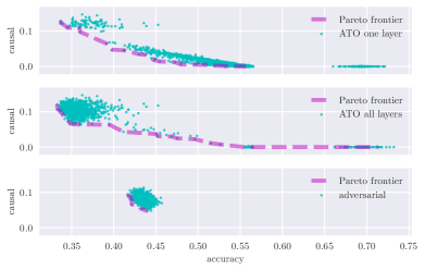
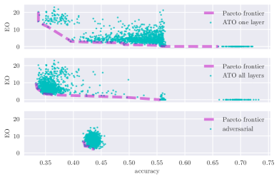
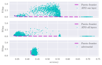
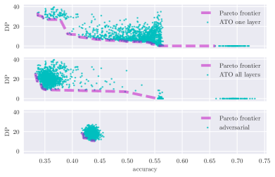
Figure 5: Pareto front estimation in the UCI (race) data set. Each three by one block corresponds to a fairness measure in Table 3 of the main document. Within each block, the row corresponds to different Pareto front estimation procedure – “ATO one layer” refers to Algorithm 1 in the main document employing the ATO causal estimand in the penultimate layer as $U_{n}$, “ATO all layers” refers to Algorithm 1 with the ATO causal estimand calculated over all layers, and lastly the adversarial approach. In each subplot, 1500 candidates are displayed along with the culled Pareto front displayed in dashed magenta.

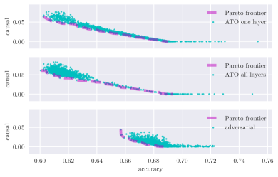
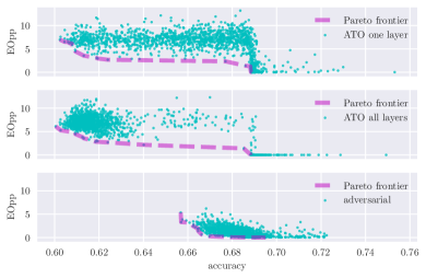
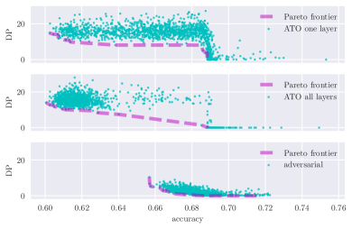
Figure 6: Pareto front estimation in the recidivism data set. Each three by one block corresponds to a fairness measure in Table 3 of the main document. Within each block, the row corresponds to different Pareto front estimation procedure – “ATO one layer” refers to Algorithm 1 in the main document employing the ATO causal estimand in the penultimate layer as $U_{n}$, “ATO all layers” refers to Algorithm 1 with the ATO causal estimand calculated over all layers, and lastly the adversarial approach. In each subplot, 1500 candidates are displayed along with the culled Pareto front displayed in dashed magenta.

We present the results for the UCI (gender) dataset in Figure 4. The results for UCI (race) and recidivism can be found in Figure 5 and Figure 6 in Appendix A, respectively. Each three-by-one block in Figure 4 corresponds to a different fairness measure $U(\theta,\hat{P}_{\rm{test}})$ in Table 3. Within each block, the rows correspond to a different approach to finding the Pareto candidates.

Since 15 values of $\lambda$ and 100 training-testing splits are considered, the output of Algorithm 1, candidates, consists in total 1500 learned network parameters. The 1500 experiments were run in parallel using high performance computing resources. It should be noted that the individual nodes used are less powerful than many personal workstations, and even so, a single training run takes only about thirty minutes.

The results of applying Algorithm 1 with $U_{n}(\theta)=\left|\hat{\tau}_{ATO}({\mathbf{h}}^{(L-1)})\right\rvert$ and $U_{n}(\theta)=\sum_{l=1}^{L-1}\left\lvert\hat{\tau}_{ATO}({\mathbf{h}}^{(l)})\right\rvert$ are shown in the first and second rows of each three-by-one block in Figure 4, respectively. In each sub-figure, we plot for each $\theta\in\textsc{candidates}$, its value in the fairness-accuracy space, $R(\theta,\hat{P}_{\rm{test}})$ versus $U(\theta,\hat{P}_{\rm{test}})$. We further display the Pareto front culled from these 1500 Pareto candidates where the culling simply discards the dominated points.

The result of the adversarial approach is displayed in the third row of each three-by-one block of Figure 4. Fifteen values of $\lambda$ in equation 9 along with 100 training-testing splits are considered, producing in total 1500 $\theta_{clf}$, each of which is plotted in the fairness-accuracy space, $R(\theta,\hat{P}_{\rm{test}})$ versus $U(\theta,\hat{P}_{\rm{test}})$.

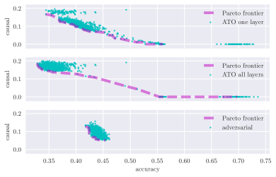
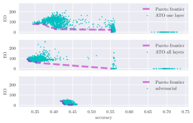
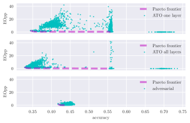
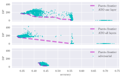
Figure 4: Pareto front estimation in the UCI (gender) test set. Each three by one block corresponds to a different fairness evaluation in Table 3. Within each block, the row corresponds to different Pareto front estimation procedures – “ATO one layer” refers to Algorithm 1 employing the ATO causal estimand in the penultimate layer as $U_{n}$, “ATO all layers” refers to Algorithm 1 with the ATO causal estimand calculated over all intermediate layers, and lastly the adversarial approach. In each subplot, 1500 candidates are displayed along with the culled Pareto front in dashed magenta. The accuracy x-axis plots $R(\theta,\hat{P}_{\rm{test}})$ and the fairness y-axis plots $U(\theta,\hat{P}_{\rm{test}})$.

We can immediately see from Figure 4 that compared to Algorithm 1, the adversarial approach is less capable of finding a Pareto front that spans the fairness-accuracy space. Indeed Table 4 shows that the set of non-dominated points found by the adversarial approach is much smaller relative to Algorithm 1.

We also observe better Pareto front estimation when Algorithm 1 is applied with $U_{n}$ as the ATO causal measure calculated in the penultimate layer, compared to the ATO calculated over all layers. This seems to be true of the two other data settings as well, as can be seen in Appendix A. This suggests using equation 8 for $U_{n}$ makes training the neural network more difficult. It may be worthwhile to explore training the network one layer at a time in future work.

Finally, from Figure 4, we can see that the demographic parity, equal odds, and equal opportunity fairness measures tend to form distinct clumps in the fairness-accuracy space, relative to the ATO causal measure. Results for UCI (race) and recidivism contained in Appendix A indicate much of the same conclusions. Appendix A also contains further visualization on the distributions of the prediction probabilities as $\lambda$ in Algorithm 1 is dialed between 0 and 1.

Table 4: Each row corresponds to a different approach of finding the fairness-accuracy Pareto front. Each column corresponds to a different dataset. The individual cells report the number of non-dominated points (higher is better) calculated in the space $(R(\theta,\hat{P}_{\rm{test}}),U(\theta,\hat{P}_{\rm{test}}))$ where $U(\theta,\hat{P}_{\rm{test}})=\left\lvert\tau_{ATO}(f_{\theta}({\mathbf{x}});\hat{P}_{\rm{test}})\right\rvert$. ATO one layer refers to Algorithm 1 where $U_{n}$ is the ATO calculated on the penultimate layer, while ATO all layers refers to the ATO calculated over all intermediate layers.

	UCI (gender)	UCI (race)	Recidivism
ATO one layer	44	33	89
ATO all layers	27	27	53
Adversarial	13	9	27

6 Future work

We have found standardization of the objectives to be crucial as a preprocessing step. Recent works such as GradNorm (Chen et al., 2018) may offer a way to simultaneously standardize as we train rather than as a preprocessing step. We also discovered that the Chebyshev scalarization scheme, though superior to the linear scalarization scheme, is still seen to often produce dominated points. This may not be a particular fault of the Chebyshev scalarization scheme, Rather the phenomenon is likely due to the fact that we can never perform optimization perfectly, especially for deep neural networks using stochastic optimization algorithms. Barring this practical difficulty, as Chebyshev scalarization only leads to weakly Pareto optimal solutions, there still may be theoretical grounds for improvement. We may do better by using e.g., the hypervolume indicator (Auger et al., 2012) to find points that are Pareto optimal. This has its own challenges, as the hypervolume indicator is expensive to calculate in higher dimensions.

Our experiments also reveal the difficulty of selecting weights in the Chebyshev scalarization scheme in such a way that would lead to a wide diversity of Pareto optimal points. In fact, many different weights often produced nearly identical solutions. Appropriately specifying the weights in a scalarization scheme without a priori information on the shape of the Pareto front itself is an open problem in multi-objective optimization. We had stated earlier that adaptive weights would be an improvement to the current methodology. This certainly merits further study but the following challenges can be anticipated. Adapting the weights while training the neural network fundamentally changes the convergence behavior of the optimization algorithm since the optimization problem itself is gradually changing. It is already a nontrivial affair to train a deep neural network, and so we expect the addition of weight adaptation will require careful tinkering to the training process. Furthermore, many adaptive weight schemes seem to depend on the Pareto front shape itself. Without a better understanding of the Pareto front, we might do more harm by using an unsuitable weight adaptation technique.

Appendix A Additional figures

In this section, we provide additional figures for the experiments conducted in “The Fairness-Accuracy Pareto Front.” Figures 5 and 6 here are analogous to Figure 4 in the main text. The figures report, respectively, the results for the UCI (race) and recidivism dataset. Within each three-by-one block, the results of various Pareto estimation procedures are reported. Each block of subfigures corresponds to a different $U(\theta;\hat{P}_{\rm{test}})$.

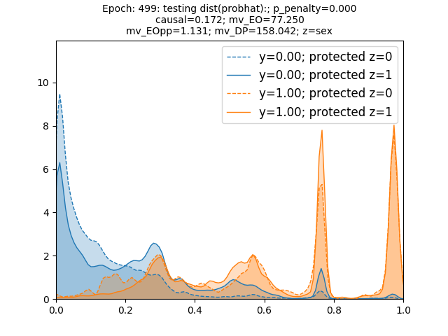
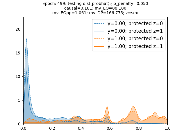
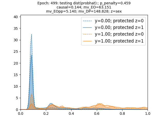
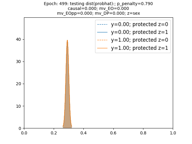
Figure 7: For a particular training-testing split of the UCI (gender) dataset, we display the distributions of the predicted probabilities in the test set for four different values of $\lambda$, where $\lambda$ is indicated by p_penalty in the heading of each plot. The distributions are broken down by different values of the true target label ${\mathbf{y}}$ and the sensitive attribute ${\mathbf{z}}$. Besides the ATO measure (causal), we also indicate equalised odds (mv_EO), equality of opportunity (mv_EOpp) and demographic parity (mv_DP) in the headings of the subplots.

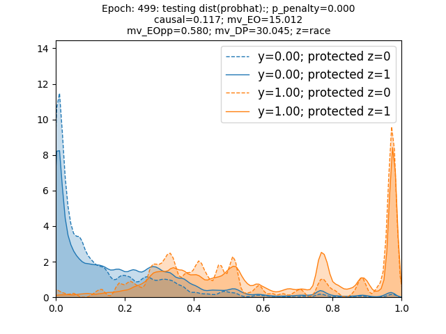
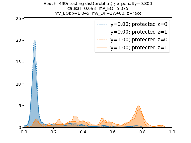
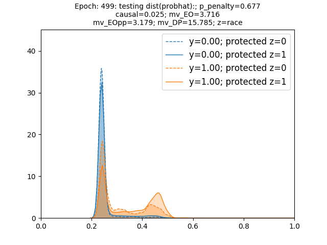
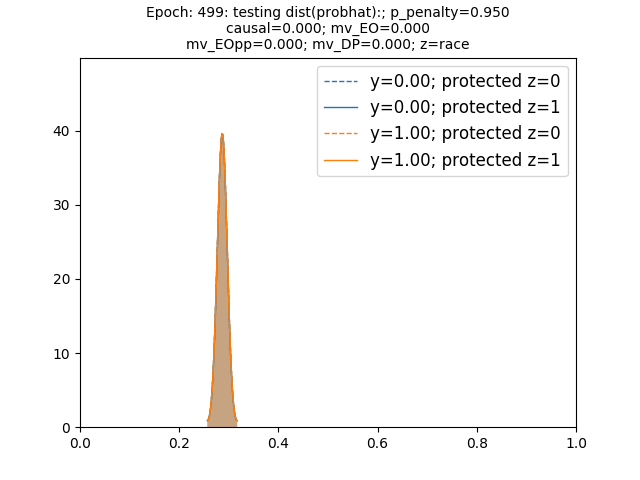
Figure 8: For a particular training-testing split of the UCI (race) dataset, we display the distributions of the predicted probabilities in the test set for four different values of $\lambda$, where $\lambda$ is indicated by p_penalty in the heading of each plot. The distributions are broken down by different values of the true target label ${\mathbf{y}}$ and the sensitive attribute ${\mathbf{z}}$. Besides the ATO measure (causal), we also indicate equalised odds (mv_EO), equality of opportunity (mv_EOpp) and demographic parity (mv_DP) in the headings of the subplots.

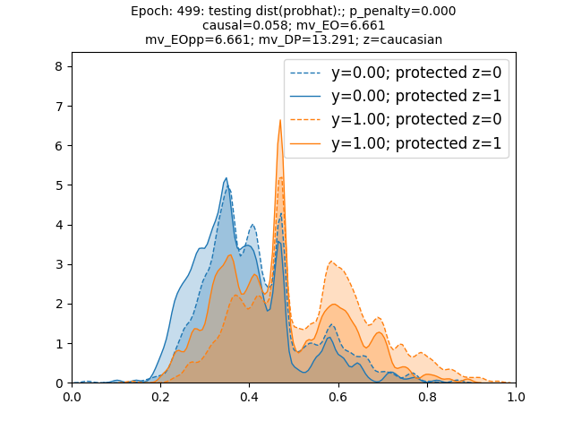
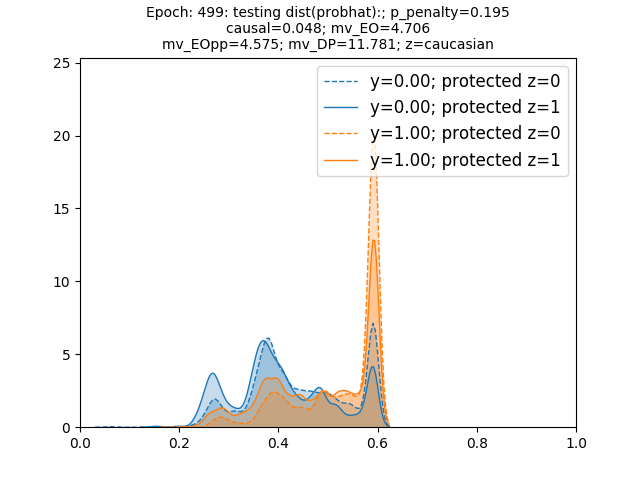
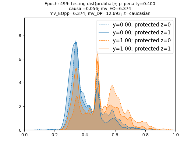
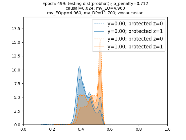
Figure 9: For a particular training-testing split of the recidivism dataset, we display the distributions of the predicted probabilities in the test set for four different values of $\lambda$, where $\lambda$ is indicated by p_penalty in the heading of each plot. The distributions are broken down by different values of the true target label ${\mathbf{y}}$ and the sensitive attribute ${\mathbf{z}}$. Besides the ATO measure (causal), we also indicate equalised odds (mv_EO), equality of opportunity (mv_EOpp) and demographic parity (mv_DP) in the headings of the subplots.

We also provide figures that help visualise the effect of dialling $\lambda$ in Algorithm 1 of the main text from 0 to 1. In Figure 7, we display the distribution of the classifier’s prediction in the UCI (gender) dataset broken down by class label and sensitive attribute. Each panel of Figure 7 is a different $\lambda$ value. In addition to reporting the ATO measure of fairness, we also indicate other non-causal fairness metrics including Equalised Odds, Equal Opportunity, and Demographic Parity. Similar visualisation for the UCI (race) and recidivism dataset can be found in Figures 8 and 9, respectively.

Appendix B Estimation of demographic and conditional parity

We describe a quantitative index that measures the degree to which conditional parity holds. First, recall we say a prediction score $\hat{S}$ exhibits conditional parity with respect to sensitive attribute $Z$ conditioned on $U$ if $Z$ and $U$ are independent conditional on $U$. We will limit the scope to categorical $U$ and categorical $Z$. The conditional independence statement $\hat{S}\mathchoice{\mathrel{\hbox to0.0pt{$\displaystyle\perp$\hss}\mkern 2.0mu{\displaystyle\perp}}}{\mathrel{\hbox to0.0pt{$\textstyle\perp$\hss}\mkern 2.0mu{\textstyle\perp}}}{\mathrel{\hbox to0.0pt{$\scriptstyle\perp$\hss}\mkern 2.0mu{\scriptstyle\perp}}}{\mathrel{\hbox to0.0pt{$\scriptscriptstyle\perp$\hss}\mkern 2.0mu{\scriptscriptstyle\perp}}}Z\mid U$ is typically assessed using the Cochran-Mantel-Haenszel test when $\hat{S}$ and $Z$ are binary variables and $U$ is another, let’s say $k$-level, categorical variable. Conditional independence in this case simply reduces to equality of odds ratios in each of the $k$ two-by-two contingency tables.

A more sophisticated method is required to assess conditional parity when $\hat{S}$ is continuous. In the following, we introduce an index for conditional parity by adapting the mean-variance statistic of  Cui et al. [2015], which is not directly applicable as it is designed for unconditional independence assessment between a continuous variable and a categorical variable.

B.1 The Mean-Variance Index

Without loss of generality, suppose the categorical random vector $Z$ takes value in the set $\{z_{1},\ldots,z_{R}\}$. Let $F_{r}(s)=P(\hat{S}\leq s\mid Z=z_{r})$ be the conditional distribution of $\hat{S}$ given $Z=z_{r}$. Let $F(s)=P(\hat{S}\leq s)$ be the unconditional distribution of $\hat{S}$. The mean-variance index Cui et al. [2015] is given by

$$MV=\sum_{r=1}^{R}P(Z=z_{r})\int[F_{r}(s)-F(s)]^{2}\,dF(s),$$ (10)

where $P(Z=z_{r})>0$ for all $j=1,\ldots,r$. Note that the integral in equation 10 is simply the Cramér-von Mises distances between $F_{r}$ and $F$, and so the mean-variance statistic is the weighted average of these distances, weighted by how likely a particular value of $Z$ is. If $\hat{S}$ and $Z$ are independent, then $F_{r}(s)=F(s)$ for all $r=1,\ldots,R$. Thus the mean-variance index in equation 10 has the salient property that it is zero if and only if $\hat{S}\mathchoice{\mathrel{\hbox to0.0pt{$\displaystyle\perp$\hss}\mkern 2.0mu{\displaystyle\perp}}}{\mathrel{\hbox to0.0pt{$\textstyle\perp$\hss}\mkern 2.0mu{\textstyle\perp}}}{\mathrel{\hbox to0.0pt{$\scriptstyle\perp$\hss}\mkern 2.0mu{\scriptstyle\perp}}}{\mathrel{\hbox to0.0pt{$\scriptscriptstyle\perp$\hss}\mkern 2.0mu{\scriptscriptstyle\perp}}}Z$.

Let the notation $1\{\cdot\}$ denote indicator function of an event, i.e. it is 1 if the event happens and 0 otherwise. The plug-in estimator for equation 10 based on a sample $\{(\hat{S}_{i},Z_{i}),i=1,\ldots,n\}$ is

$$\widehat{MV}=\sum_{r=1}^{R}\hat{P}(Z=z_{r})\left[\frac{1}{n}\sum_{i=1}^{n}[\hat{F}_{r}(\hat{S}_{i})-\hat{F}(\hat{S}_{i})]^{2}\right]$$ (11)

where

$$\hat{P}(Z=z_{r}) =n^{-1}\sum_{i=1}^{n}1\{Z_{i}=z_{r}\},$$

$$\hat{F}_{r}(s) =\frac{\sum_{i=1}^{n}1\{\hat{S}_{i}\leq s,Z_{i}=z_{r}\}}{\sum_{i=1}^{n}1\{Z_{i}=z_{r}\}},$$

$$\hat{F}(s) =\frac{1}{n}\sum_{i=1}^{n}1\{\hat{S}_{i}\leq s\}.$$

That the estimator in equation 11 is consistent for its theoretical counterpart in equation 10, i.e. $\widehat{MV}$ converges in probability to $MV$ as $n\to\infty$, is established in Cui et al. [2015].

B.2 A new index to measure conditional parity

Now let us return to the assessment of $\hat{S}\mathchoice{\mathrel{\hbox to0.0pt{$\displaystyle\perp$\hss}\mkern 2.0mu{\displaystyle\perp}}}{\mathrel{\hbox to0.0pt{$\textstyle\perp$\hss}\mkern 2.0mu{\textstyle\perp}}}{\mathrel{\hbox to0.0pt{$\scriptstyle\perp$\hss}\mkern 2.0mu{\scriptstyle\perp}}}{\mathrel{\hbox to0.0pt{$\scriptscriptstyle\perp$\hss}\mkern 2.0mu{\scriptscriptstyle\perp}}}Z\mid U$. Suppose the categorical random vector $U$ takes value in the set $\{u_{1},\ldots,u_{K}\}$. Then we propose the following as a direct extension of the mean-variance statistic of Cui et al. [2015] to the conditional case:

$$MV^{k}=\sum_{r=1}^{R}P_{k}(Z=z_{r})\int[F_{r,k}(s)-F_{k}(s)]^{2}\,dF_{k}(s)$$ (12)

where

$$P_{k}(Z=z_{r}) =P(Z=z_{r}\mid U=u_{k})$$

$$F_{r,k}(s) =P(\hat{S}\leq s\mid Z=z_{r},U=u_{k})$$

$$F_{k}(s) =P(\hat{S}\leq s\mid U=u_{k}).$$

We employ the following statistic to assess the degree to which $\hat{S}\mathchoice{\mathrel{\hbox to0.0pt{$\displaystyle\perp$\hss}\mkern 2.0mu{\displaystyle\perp}}}{\mathrel{\hbox to0.0pt{$\textstyle\perp$\hss}\mkern 2.0mu{\textstyle\perp}}}{\mathrel{\hbox to0.0pt{$\scriptstyle\perp$\hss}\mkern 2.0mu{\scriptstyle\perp}}}{\mathrel{\hbox to0.0pt{$\scriptscriptstyle\perp$\hss}\mkern 2.0mu{\scriptscriptstyle\perp}}}Z\mid U$ holds:

$$\max_{k=1,\ldots,K}MV^{k}(\hat{S},Z).$$ (13)

Since $MV^{k}$ is zero if and only if $\hat{S}$ is independent of $Z$ conditioned on $U$ and the same is true for the maximum. In other words, equation 13 is zero if and only if $\hat{S}\mathchoice{\mathrel{\hbox to0.0pt{$\displaystyle\perp$\hss}\mkern 2.0mu{\displaystyle\perp}}}{\mathrel{\hbox to0.0pt{$\textstyle\perp$\hss}\mkern 2.0mu{\textstyle\perp}}}{\mathrel{\hbox to0.0pt{$\scriptstyle\perp$\hss}\mkern 2.0mu{\scriptstyle\perp}}}{\mathrel{\hbox to0.0pt{$\scriptscriptstyle\perp$\hss}\mkern 2.0mu{\scriptscriptstyle\perp}}}Z\mid U$.

Since equation 12 and equation 13 are both unknown population quantities, they require estimation. Let $\widehat{MV_{k}}$ be the plug-in estimator for equation 12 based on the empirical measure. Namely, let

$$\widehat{MV^{k}}(\hat{S},Z)=\sum_{r=1}^{R}\hat{P}_{k}(Z=z_{r})\int[\hat{F}_{r,k}(s)-\hat{F}_{k}(s)]^{2}\,d\hat{F}_{k}(s)$$

where

$$\hat{P}_{k}(Z=z_{r}) =\frac{\sum_{i=1}^{n}1\{Z_{i}=z_{r},U_{i}=u_{k}\}}{\sum_{i=1}^{n}1\{U_{i}=u_{k}\}}$$

$$\hat{F}_{r,k}(s) =\frac{\sum_{i=1}^{n}1\{\hat{S}_{i}\leq s,Z_{i}=z_{r},U_{i}=u_{k}\}}{\sum_{i=1}^{n}1\{Z_{i}=z_{r},U_{i}=u_{k}\}}$$

$$\hat{F}_{k}(s) =\frac{\sum_{i=1}^{n}1\{\hat{S}_{i}\leq s,U_{i}=u_{k}\}}{\sum_{i=1}^{n}1\{U_{i}=u_{k}\}}.$$

To estimate equation 13, we simply take the maximum over $k$:

$$\max_{k=1,\ldots,K}\widehat{MV^{k}}.$$ (14)

We will call the quantity in equation 14 the conditional mean-variance index. Note that this measure will be zero if conditional independence holds and will increase with increasing dependence. Hence, it is a suitable measure to assess conditional parity.

References

- Agarwal et al. (2018) Alekh Agarwal, Alina Beygelzimer, Miroslav Dudík, John Langford, and Hanna M. Wallach. A reductions approach to fair classification. In Proceedings of the 35th International Conference on Machine Learning, ICML 2018, Stockholmsmässan, Stockholm, Sweden, July 10-15, 2018, pages 60–69, 2018. URL http://proceedings.mlr.press/v80/agarwal18a.html.
- Auger et al. (2012) Anne Auger, Johannes Bader, Dimo Brockhoff, and Eckart Zitzler. Hypervolume-based multiobjective optimization: Theoretical foundations and practical implications. Theoretical Computer Science, 425:75–103, March 2012. ISSN 0304-3975. doi: 10.1016/j.tcs.2011.03.012. URL http://www.sciencedirect.com/science/article/pii/S0304397511002428.
- Bechavod and Ligett (2017) Yahav Bechavod and Katrina Ligett. Learning fair classifiers: A regularization-inspired approach. CoRR, abs/1707.00044, 2017.
- Berk et al. (2017) Richard Berk, Hoda Heidari, Shahin Jabbari, Matthew Joseph, Michael J. Kearns, Jamie Morgenstern, Seth Neel, and Aaron Roth. A convex framework for fair regression. CoRR, abs/1706.02409, 2017. URL http://arxiv.org/abs/1706.02409.
- Beutel et al. (2017) Alex Beutel, Jilin Chen, Zhe Zhao, and Ed Huai hsin Chi. Data decisions and theoretical implications when adversarially learning fair representations. CoRR, abs/1707.00075, 2017.
- Bickel et al. (1975) Peter J Bickel, Eugene A Hammel, and J William O’Connell. Sex bias in graduate admissions: Data from berkeley. Science, 187(4175):398–404, 1975.
- Calders and Verwer (2010) Toon Calders and Sicco Verwer. Three naive bayes approaches for discrimination-free classification. Data Mining and Knowledge Discovery, 21(2):277–292, Sep 2010. ISSN 1573-756X. doi: 10.1007/s10618-010-0190-x. URL https://doi.org/10.1007/s10618-010-0190-x.
- Calmon et al. (2017) Flavio Calmon, Dennis Wei, Bhanukiran Vinzamuri, Karthikeyan Natesan Ramamurthy, and Kush R Varshney. Optimized pre-processing for discrimination prevention. In I. Guyon, U. V. Luxburg, S. Bengio, H. Wallach, R. Fergus, S. Vishwanathan, and R. Garnett, editors, Advances in Neural Information Processing Systems 30, pages 3992–4001. Curran Associates, Inc., 2017. URL http://papers.nips.cc/paper/6988-optimized-pre-processing-for-discrimination-prevention.pdf.
- Chen et al. (2018) Zhao Chen, Vijay Badrinarayanan, Chen-Yu Lee, and Andrew Rabinovich. Gradnorm: Gradient normalization for adaptive loss balancing in deep multitask networks. In International Conference on Machine Learning, pages 794–803. PMLR, 2018.
- Cui et al. (2015) Hengjian Cui, Runze Li, and Wei Zhong. Model-free feature screening for ultrahigh dimensional discriminant analysis. Journal of the American Statistical Association, 110 510:630–641, 2015.
- Das and Dennis (1997) I. Das and J. E. Dennis. A closer look at drawbacks of minimizing weighted sums of objectives for pareto set generation in multicriteria optimization problems. Structural optimization, 14(1):63–69, Aug 1997. ISSN 1615-1488. doi: 10.1007/BF01197559. URL https://doi.org/10.1007/BF01197559.
- Das and Dennis (2000) Indraneel Das and J Dennis. Normal-boundary intersection: A new method for generating the pareto surface in nonlinear multicriteria optimization problems. SIAM Journal on Optimization, 8, 07 2000. doi: 10.1137/S1052623496307510.
- Ehrgott (2000) M. Ehrgott. Multicriteria optimization. Lecture Notes in Economics and Mathematical Systems. Springer-Verlag, 2000.
- Emmerich and Deutz (2018) Michael TM Emmerich and André H Deutz. A tutorial on multiobjective optimization: fundamentals and evolutionary methods. Natural computing, 17(3):585–609, 2018.
- Feldman et al. (2015) Michael Feldman, Sorelle A. Friedler, John Moeller, Carlos Scheidegger, and Suresh Venkatasubraan. Certifying and removing disparate impact. In Proceedings of the 21th ACM SIGKDD International Conference on Knowledge Discovery and Data Mining, KDD ’15, pages 259–268, New York, NY, USA, 2015. ACM. ISBN 978-1-4503-3664-2. doi: 10.1145/2783258.2783311. URL http://doi.acm.org/10.1145/2783258.2783311.
- Giagkiozis and Fleming (2015) I. Giagkiozis and P.J. Fleming. Methods for multi-objective optimization: An analysis. Information Sciences, 293:338 – 350, 2015. ISSN 0020-0255. doi: https://doi.org/10.1016/j.ins.2014.08.071. URL http://www.sciencedirect.com/science/article/pii/S0020025514009074.
- Guo et al. (2017) Chuan Guo, Geoff Pleiss, Yu Sun, and Kilian Q. Weinberger. On calibration of modern neural networks. In Proceedings of the 34th International Conference on Machine Learning - Volume 70, ICML’17, pages 1321–1330. JMLR.org, 2017. URL http://dl.acm.org/citation.cfm?id=3305381.3305518.
- Hardt et al. (2016) Moritz Hardt, Eric Price, and Nathan Srebro. Equality of opportunity in supervised learning. In Proceedings of the 30th International Conference on Neural Information Processing Systems, NIPS’16, pages 3323–3331, USA, 2016. Curran Associates Inc. ISBN 978-1-5108-3881-9. URL http://dl.acm.org/citation.cfm?id=3157382.3157469.
- Imbens and Rubin (2015) Guido W. Imbens and Donald B. Rubin. Causal Inference for Statistics, Social, and Biomedical Sciences: An Introduction. Cambridge University Press, New York, NY, USA, 2015. ISBN 0521885884, 9780521885881.
- Johndrow and Lum (2019) James E. Johndrow and Kristian Lum. An algorithm for removing sensitive information: Application to race-independent recidivism prediction. Ann. Appl. Stat., 13(1):189–220, 03 2019. doi: 10.1214/18-AOAS1201. URL https://doi.org/10.1214/18-AOAS1201.
- Joseph et al. (2016) Matthew Joseph, Michael Kearns, Jamie H Morgenstern, and Aaron Roth. Fairness in learning: Classic and contextual bandits. In D. D. Lee, M. Sugiyama, U. V. Luxburg, I. Guyon, and R. Garnett, editors, Advances in Neural Information Processing Systems 29, pages 325–333. Curran Associates, Inc., 2016. URL http://papers.nips.cc/paper/6355-fairness-in-learning-classic-and-contextual-bandits.pdf.
- Kamiran and Calders (2012) Faisal Kamiran and Toon Calders. Data preprocessing techniques for classification without discrimination. Knowledge and Information Systems, 33(1):1–33, Oct 2012. ISSN 0219-3116. doi: 10.1007/s10115-011-0463-8. URL https://doi.org/10.1007/s10115-011-0463-8.
- Kamishima et al. (2011) Toshihiro Kamishima, Shotaro Akaho, and Jun Sakuma. Fairness-aware learning through regularization approach. In Proceedings of the 2011 IEEE 11th International Conference on Data Mining Workshops, ICDMW ’11, pages 643–650, Washington, DC, USA, 2011. IEEE Computer Society. ISBN 978-0-7695-4409-0. doi: 10.1109/ICDMW.2011.83. URL https://doi.org/10.1109/ICDMW.2011.83.
- Khademi et al. (2019) Aria Khademi, Sanghack Lee, David Foley, and Vasant Honavar. Fairness in algorithmic decision making: An excursion through the lens of causality. In The World Wide Web Conference, WWW ’19, pages 2907–2914, New York, NY, USA, 2019. ACM. ISBN 978-1-4503-6674-8. doi: 10.1145/3308558.3313559. URL http://doi.acm.org/10.1145/3308558.3313559.
- Kilbertus et al. (2017) Niki Kilbertus, Mateo Rojas-Carulla, Giambattista Parascandolo, Moritz Hardt, Dominik Janzing, and Bernhard Schölkopf. Avoiding discrimination through causal reasoning. In Proceedings of the 31st International Conference on Neural Information Processing Systems, NIPS’17, pages 656–666, USA, 2017. Curran Associates Inc. ISBN 978-1-5108-6096-4. URL http://dl.acm.org/citation.cfm?id=3294771.3294834.
- Kingma and Ba (2014) Diederik Kingma and Jimmy Ba. Adam: A method for stochastic optimization. International Conference on Learning Representations, 12 2014.
- Kleinberg (2018) Jon Kleinberg. Inherent trade-offs in algorithmic fairness. In Abstracts of the 2018 ACM International Conference on Measurement and Modeling of Computer Systems, SIGMETRICS ’18, pages 40–40, New York, NY, USA, 2018. ACM. ISBN 978-1-4503-5846-0. doi: 10.1145/3219617.3219634. URL http://doi.acm.org/10.1145/3219617.3219634.
- Kusner et al. (2017) Matt J Kusner, Joshua Loftus, Chris Russell, and Ricardo Silva. Counterfactual fairness. In I. Guyon, U. V. Luxburg, S. Bengio, H. Wallach, R. Fergus, S. Vishwanathan, and R. Garnett, editors, Advances in Neural Information Processing Systems 30, pages 4066–4076. Curran Associates, Inc., 2017. URL http://papers.nips.cc/paper/6995-counterfactual-fairness.pdf.
- Li et al. (2014) Cong Li, Michael Georgiopoulos, and Georgios C Anagnostopoulos. Pareto-path multitask multiple kernel learning. IEEE transactions on neural networks and learning systems, 26(1):51–61, 2014.
- Li et al. (2018) Fan Li, Kari Lock Morgan, and Alan M. Zaslavsky. Balancing covariates via propensity score weighting. Journal of the American Statistical Association, 113(521):390–400, 2018. doi: 10.1080/01621459.2016.1260466. URL https://doi.org/10.1080/01621459.2016.1260466.
- Lin et al. (2019) Xi Lin, Hui-Ling Zhen, Zhenhua Li, Qing-Fu Zhang, and Sam Kwong. Pareto multi-task learning. In Advances in Neural Information Processing Systems, pages 12060–12070, 2019.
- Loftus et al. (2018) Joshua R. Loftus, Chris Russell, Matt J. Kusner, and Ricardo Silva. Causal reasoning for algorithmic fairness. CoRR, abs/1805.05859, 2018. URL http://arxiv.org/abs/1805.05859.
- Louppe et al. (2017) Gilles Louppe, Michael Kagan, and Kyle Cranmer. Learning to pivot with adversarial networks. In I. Guyon, U. V. Luxburg, S. Bengio, H. Wallach, R. Fergus, S. Vishwanathan, and R. Garnett, editors, Advances in Neural Information Processing Systems 30, pages 981–990. Curran Associates, Inc., 2017. URL http://papers.nips.cc/paper/6699-learning-to-pivot-with-adversarial-networks.pdf.
- Madras et al. (2018) David Madras, Elliot Creager, Toniann Pitassi, and Richard Zemel. Learning adversarially fair and transferable representations. In Jennifer Dy and Andreas Krause, editors, Proceedings of the 35th International Conference on Machine Learning, volume 80 of Proceedings of Machine Learning Research, pages 3384–3393, Stockholmsmassan, Stockholm Sweden, 10–15 Jul 2018. PMLR. URL http://proceedings.mlr.press/v80/madras18a.html.
- Manisha and Gujar (2018) P. Manisha and Sujit Gujar. A neural network framework for fair classifier. CoRR, abs/1811.00247, 2018. URL http://arxiv.org/abs/1811.00247.
- Moffaert and Nowe (2014) Kristof Van Moffaert and Ann Nowe. Multi-Objective Reinforcement Learning using Sets of Pareto Dominating Policies. Journal of Machine Learning Research, 15, 2014.
- Narasimhan (2018) Harikrishna Narasimhan. Learning with complex loss functions and constraints. In Amos Storkey and Fernando Perez-Cruz, editors, Proceedings of the Twenty-First International Conference on Artificial Intelligence and Statistics, volume 84 of Proceedings of Machine Learning Research, pages 1646–1654, Playa Blanca, Lanzarote, Canary Islands, 09–11 Apr 2018. PMLR. URL http://proceedings.mlr.press/v84/narasimhan18a.html.
- Ritov et al. (2017) Ya’acov Ritov, Yuekai Sun, and Ruofei Zhao. On conditional parity as a notion of non-discrimination in machine learning. To appear in Statistical Science, 2017.
- Sener and Koltun (2018) Ozan Sener and Vladlen Koltun. Multi-task learning as multi-objective optimization. In Advances in Neural Information Processing Systems, pages 527–538, 2018.
- Shah and Ghahramani (2016) Amar Shah and Zoubin Ghahramani. Pareto frontier learning with expensive correlated objectives. In International Conference on Machine Learning, pages 1919–1927, 2016.
- Wadsworth et al. (2018) Christina Wadsworth, Francesca Vera, and Chris Piech. Achieving fairness through adversarial learning: an application to recidivism prediction. CoRR, abs/1807.00199, 2018. URL http://arxiv.org/abs/1807.00199.
- Yaochu Jin and Sendhoff (2008) Yaochu Jin and B. Sendhoff. Pareto-Based Multiobjective Machine Learning: An Overview and Case Studies. IEEE Transactions on Systems, Man, and Cybernetics, Part C (Applications and Reviews), 38(3):397–415, May 2008. ISSN 1094-6977. doi: 10.1109/TSMCC.2008.919172. URL http://ieeexplore.ieee.org/document/4492360/.
- Zafar et al. (2017a) Muhammad Bilal Zafar, Isabel Valera, Manuel Gomez-Rodriguez, and Krishna P. Gummadi. Fairness constraints: Mechanisms for fair classification. In Proceedings of the 20th International Conference on Artificial Intelligence and Statistics, AISTATS 2017, 20-22 April 2017, Fort Lauderdale, FL, USA, pages 962–970, 2017a. URL http://proceedings.mlr.press/v54/zafar17a.html.
- Zafar et al. (2017b) Muhammad Bilal Zafar, Isabel Valera, Manuel Gomez Rodriguez, and Krishna P. Gummadi. Fairness beyond disparate treatment & disparate impact: Learning classification without disparate mistreatment. In Proceedings of the 26th International Conference on World Wide Web, WWW ’17, pages 1171–1180, Republic and Canton of Geneva, Switzerland, 2017b. International World Wide Web Conferences Steering Committee. ISBN 978-1-4503-4913-0. doi: 10.1145/3038912.3052660. URL https://doi.org/10.1145/3038912.3052660.
- Zafar et al. (2017c) Muhammad Bilal Zafar, Isabel Valera, Manuel Gomez Rodriguez, Krishna P. Gummadi, and Adrian Weller. From parity to preference-based notions of fairness in classification. In Proceedings of the 31st International Conference on Neural Information Processing Systems, NIPS’17, pages 228–238, Red Hook, NY, USA, 2017c. Curran Associates Inc. ISBN 9781510860964.
- Zhang and Golovin (2020) Richard Zhang and Daniel Golovin. Random hypervolume scalarizations for provable multi-objective black box optimization. In International Conference on Machine Learning, pages 11096–11105. PMLR, 2020.