Deep Variational Network Toward
Blind Image Restoration

Abstract

Blind image restoration (IR) is a common yet challenging problem in computer vision. Classical model-based methods and recent deep learning (DL)-based methods represent two different methodologies for this problem, each with their own merits and drawbacks. In this paper, we propose a novel blind image restoration method, aiming to integrate both the advantages of them. Specifically, we construct a general Bayesian generative model for the blind IR, which explicitly depicts the degradation process. In this proposed model, a pixel-wise non-i.i.d. Gaussian distribution is employed to fit the image noise. It is with more flexibility than the simple i.i.d. Gaussian or Laplacian distributions as adopted in most of conventional methods, so as to handle more complicated noise types contained in the image degradation. To solve the model, we design a variational inference algorithm where all the expected posteriori distributions are parameterized as deep neural networks to increase their model capability. Notably, such an inference algorithm induces a unified framework to jointly deal with the tasks of degradation estimation and image restoration. Further, the degradation information estimated in the former task is utilized to guide the latter IR process. Experiments on two typical blind IR tasks, namely image denoising and super-resolution, demonstrate that the proposed method achieves superior performance over current state-of-the-arts. The source code is available at https://github.com/zsyOAOA/VIRNet.

1 Introduction

Image restoration (IR) is an active research topic in the fields of signal processing and computer vision. It aims at recovering the latent high-quality image $\bm{z}$ from the observed corrupted counterpart $\bm{y}$, i.e.,

$$\bm{y}=H\bm{z}+\bm{n},$$ (1)

where $H$ is the degradation operator, and $\bm{n}$ is image noise. With different degradation settings for $H$, Eq. (1) represents different IR tasks. For example, the classical IR tasks, such as image denoising, deblurring, and super-resolution, can be easily obtained by setting $H$ as an identity matrix, a blurring operator, and a composition of blurring and downsampling operators, respectively. The difficulties of IR tasks mainly come from $H$ and $\bm{n}$. The former inclines to cause severe information loss in some tasks, like deblurring and super-resolution, and the latter is usually complicated due to the accumulation of noises from multiple sourcesm e.g., capturing instrument, camera pipeline and image transmission [1]. In blind IR tasks, we need to simultaneously solve the problems of degradation estimation and image restoration, which makes it more challenging.

In the past decades, plenty of IR methods have been proposed under the maximum a posteriori (MAP) framework. From the Bayesian perspective, it generally involves a likelihood term and a prior term. More specifically, the likelihood term encodes the image degradation process of Eq. (1), while the prior term reflects our subjective knowledge on the latent high-quality image. Most of these methods mainly focused on designing more effective image priors so as to alleviate the ill-posedness of IR tasks. Commonly used image priors include total variation (TV) [2], non-local similarity [3, 4], sparsity [5, 6, 7], low-rankness [8, 9, 10] and so on. In contrast, other works focused on the likelihood term by constructing more flexible noise distributions, e.g., mixture of Gaussian (MoG) [11], mixture of Exponential (MoEP) [12], and Dirichlet Process mixture of Gaussian (DP-MoG) [13, 14, 15]. Even though these model-based methods are with highly intuitive physical meanings and also generalize well in most of scenarios, they still have evident defects. Firstly, these methods are always time-consuming, since they require to re-solve the whole model for any new testing images. Such one-by-one optimized paradigm tends to bring up large computational burden, making them very hard to be applied in real applications. Secondly, limited by the manually designed likelihood and image priors, which usually cannot faithfully represent the image knowledges, they struggle to handle some complex modeling problems in real cases, such as the blind IR tasks with complicated image degradations.

Different from the aforementioned model-based methods, current deep learning (DL)-based methods represent another research trend. Their core idea is to employ the deep neural networks (DNNs), being with powerful fitting capability, to directly learn the image knowledge from large amount of pre-collected image pairs in an end-to-end training manner. Dong et al. [16] and Zhang et al. [17] firstly proposed SRCNN and DnCNN that surpassed classical model-based methods in image super-resolution and denoising, respectively. Subsequently, many DL-based methods [18, 19, 20, 21, 22, 23, 24, 25, 26] were proposed and they achieved unprecedent successes in the field of IR. While they have achieved huge boost in performance, most of them ignore the modeling mechanism underlying the image degradation, especially the image noise. To be specific, the $L_{2}$ or $L_{1}$ losses commonly-used in current DL-based methods indeed imply that the noise $\bm{n}$ in Eq. (1) obeys the independent and identically distributed (i.i.d.) Gaussian or Laplacian distributions. This, however, always deviates from true noise configurations in real cases. For example, the camera sensor noises in practical image denoising are signal-dependent and spatially variant, and thus evidently non-i.i.d. in statistics. Neglecting such intrinsic noise properties will centainly harm the generalization capability of the model in real scenarios with complicated noises.

As analyzed above, the model-based methods are capable of encoding the image degradation through the likelihood, but hindered by the limited model capacity and the slow inference speed. In contrast, the DL-based methods, equipped with DNNs, are with large model capacity and powerful non-linear fitting capability. What’s more, in the testing phase, these methods are much faster than the model-based method, since they only need one feedforward pass for any newly coming image. This naturally inspires us to develop a new IR method, which is expected to combine both the advantages of the classical model-based methods and recent DL-based methods. In this work, we take one step forward along this research line by proposing a deep variational model for blind IR. It firstly constructs a traditional probabilistic model for IR, and then embeds the powerful DNNs into its posteriori inference to increase the model capacity. Specifically, the contributions of this work can be summarized from two aspects, namely model construction and algorithm design, as follows:

On one hand, a Bayesian generative model is built for general IR tasks, and thus naturally inherits the advantages of classical model-based methods. Furthermore, we also consider more complicated degradation process when building our model in this study:

• Instead of the simple i.i.d. Gaussian or Laplacian noise assumptions in most of the current methods, a pixel-wise non-i.i.d. distribution is adopted in our model to handle more complicated noise types. In essence, such noise model induces a learnable re-weighted loss purely relying on data-self, thus is more flexible.

• A concise kernel prior is specifically designed for super-resolution, which makes our model able to deal with the task of blind image super-resolution.

On the other hand, we elaborately design an amortized variational inference (VI) algorithm to solve the proposed generative model. Compared with the classical mean field VI methodology, two-fold substantial modifications are made to better comply with blind IR tasks:

• Different from the commonly used independent factorization strategy in VI, we factorize the expected posterior, namely the joint distribution of the degradation information and the latent clean image, into a conditional form. Such a formulation derives a unified framework to simultaneously deal with the tasks of degradation estimation and image restoration, in which the degradation information estimated by the former provides sound guidance for the subsequent restoration task.

• To largely increase the fitting capability of our model, the desirable posteriori distributions are parameterized by DNNs, and then optimized in an amortized manner during training. In the testing phase, the well-trained model is capable of fastly inferring the posteriori distribution of any new testing image in an explicit manner, and thus evidently more efficient than the classical model-based methods.

In summary, this work aims to explore a novel modeling paradigm, which is expected to integrate the merits both of the classical model-based methods and recent DL-based methods, for the IR problem. A preliminary version of this work has been published in NeurIPS 2019 [27] which focuses only on image denoising. This present work makes substantial improvements on model construction, the inference algorithm, and the empirical evaluations over the conference version. Especially, we consider a more general degradation process (i.e., Eq. (1)) to build the Bayesian generative model, making it capable of handling more complicated and general IR tasks, such as blind image super-resolution.

The remainder of the paper is organized as follows: Section 2 introduces the related work. Section 3 proposes our generative model, and discusses two typical IR tasks. Section 4 presents the designed stochastic VI algorithm for solving our model. In Section 5, experiments are demonstrated to evaluate the performance of our method. Section 6 finally concludes the paper.

2 Related Works

In this section, we firstly review model-based and DL-based IR methods. We then briefly summarize recent explorations that attempts to combine both of these two methodologies.

2.1 Model-based Methods

Most of the classical model-based methods can be formulated into the MAP framework, which contains a likelihood (fidelity) term and a prior (regularization) term from the Bayesian perspective. Relevant developments thus mainly focused on these two terms.

Prior Modeling Methods. Aiming at alleviating the ill-posed issue of IR, many studies attempted to exploit rational image prior knowledge. Statistical regularities exhibited in images were firstly employed, e.g., TV denoising [2] and wavelet coring [28]. Then, NLM [3] and BM3D [4] were both proposed for denoising based on the non-local self-similarity prior, meaning that small image patches in a non-local image area possess similar configurations. Later, low-rankness [8, 9, 10] and sparsity [5, 4, 6, 7] priors, which also aim to explore the characteristics of image patches, became popular and were widely used in IR tasks. To further increase the model’s capacity and expression ability, some other methods moved from analytical technologies to data-driven approaches. E.g., Roth and Black [29] proposed the fields of experts (FoE) to learn image priors. Barbu [30] trained a discriminative model for the Markov random field (MRF) prior, while Sun and Tappen [31] proposed a non-local range MRF (NLR-MRF) model. More related works can be found in [32, 33].

Noise Modeling Methods. Different from the prior modeling methods, noise modeling methods focus on the likelihood (fidelity) term of the MAP framework. In fact, the widely used $L_{1}$ or $L_{2}$ loss functions implicitly make the i.i.d. Gaussian or Laplacian assumptions on image noise, which often under-estimates the complexity of real noise. Based on this observation, Meng et al. [11] proposed the MoG noise modeling method under the low-rankness framework. Furthermore, Zhu et al. [34, 13] and Yue et al. [14, 15] both introduced the non-parametric Dirichlet Process into MoG to increase its flexibility, leading to the adaptive adjustment for the component number of MoG.

2.2 DL-based Methods

DL-based methods represent a data-driven trend for the IR task. They straightforwardly train an explicit mapping function parameterized by DNN on large amount of image pairs. The earliest convolutional neural network (CNN) method can be traced back to [35], in which a five-layer network was employed. Some auto-encoder based methods were then proposed in [36, 37]. Due to the insufficient research of DL technologies, however, these methods were inferior to the model-based methods in performance.

The first significant improvement of DL-based methods was achieved by [38] which obtained comparable performance with BM3D [4] in denoising task using a plain multilayer perceptron. Subsequently, Dong et al. [16] proposed the first CNN model for super-resolution, and it outperformed the classical model-based methods. With the advances of deep learning, Zhang et al. [17] trained a deep CNN model named DnCNN and achieved state-of-the-art performance in denoising, JPEG deblocking, and super-resolution. Since then, the DL-based methods began to dominate the research trend in almost all of the IR tasks, especially in denoising [18, 20, 39, 23, 25] and super-resolution [40, 41, 42, 43, 44, 45, 46].

Inspired by the development of generative adversial network (GAN) [47], some DL-based methods also followed the research line of noise modeling introduced in Sec. 2.1. Typically, Chen et al. [48] proposed a noise generator to simulate the real noise under the adversial training mechanism, and Kim et al. [49] further introduced some camera settings (e.g., ISO level and shutter speed) into the generator as extra guidance. More recently, Yue et al. [24] proposed a dual adversial loss to implement the noise removal and noise generation tasks into one unique Bayesian framework. Different from these GAN based implicit noise modeling manners, this study adopts a more powerful and flexible non-i.i.d. Gaussian distribution to explicitly model the image noise, which avoids the instability in training GAN.

2.3 Some Relevant Explorations

The researches to combine the model-based methods and the DL-based methods have attracted increasingly attentions in recent years. Some significant explorations have been attempted towards this goal.

Deep plug-and-play methods [50, 51, 52, 53, 54] usually replace the denoising subproblem in model-based methods with one or multiple pre-trained DNN denoisers, so as to leverage the abundant image prior knowledge learned by such deep denoisers. Due to the lacking of end-to-end training, they always rely on tedious hyper-parameters tuning to guarantee stable performance. To alleviate this drawback, deep unfolding methods [55, 56, 57, 58, 59] take a step forward by embedding the DNNs into traditional optimization algorithms (e.g., HQS, ADMM). Attributed to the end-to-end training manner, these deep unfolding method achieve promising performance in some IR tasks.

Deep image prior (DIP) [60] and its related methods [61, 62, 63, 64] represent another significant approach along this research line. These methods aim to seek a corresponding DNN model that maps the pre-sampled noise to the desirable clean image for any given corrupted image under the MAP framework. Similar to the model-based methods, they are mainly limited by the time-consuming optimization process in the testing phase.

In this study, we develop a general and novel deep IR model which is evidently different from the above research approaches. From the model perspective, a Bayesian generative model is constructed for general IR tasks, naturally inheriting the capability of modeling the image degradation from the classical model-based methods. From the algorithm perspective, we design an amortized VI algorithm which parameterizes all the involved posteriori distributions with DNNs. The embedded DNNs in our algorithm equip it with powerful fitting ability and fast testing speed as recent DL-based methods.

3 The Proposed Method

3.1 Basic Settings

In this paper, we consider two commonly used settings on the degradation operator $H$ of Eq. (1). In the first case, $H$ is an identity matrix, corresponding to the task of image denoising. The difficulties of this task are naturally attributed to the complexity of the image noise, which is often spatially variant and signal-dependent in real scenarios. Besides, their statistics (e.g., the noise levels) are always unknown in blind image denoising. It is thus necessary to devise methods to estimate the noise distribution and recover the latent high-quality image simultaneously.

In the second case, we consider a more general IR task, namely image super-resolution, in which $H$ is a composition of blurring and downsampling. The downsampling operation leads to serious information lost, especially in the case of large scale factor, making it more challenging compared with denoising. Similarly, blind super-resolution also involves two subtasks, i.e., estimating the degradation information, including both of the blue kernel and noise distribution, and restoring the high-resolution image.

In addition, we briefly introduce some necessary settings on the training and testing data. The training data consists of multiple triplets, i.e., $\mathcal{D}=\{\bm{y}^{(j)},\bm{x}^{(j)},H^{(j)}\}_{j=1}^{N}$, where $\bm{y}^{(j)}$ and $\bm{x}^{(j)}$ denote the corrupted image and the underlying high-quality image, respectively. $H^{(j)}$ represents the degradation operator, which is an identity matrix for denoising and a blur kernel for super-resolution. The superscript $j$ of $H^{(j)}$ indicates that the degradation model varies from one sample to another in our training data. It should be noted that, in the real-world image denoising task, $\bm{x}^{(j)}$ is usually estimated by averaging several noisy images taken under the same camera conditions [65]. In the testing phase, given only one corrupted image, our goal is to firstly estimate the degradation information, and then recover the high-quality image based on such information.

Next, we formulate a rational Bayesian generative model for the tasks of denoising and super-resolution.

3.2 Model Formulation for Denoising

Let $\{\bm{y},\bm{x}\}\in\mathcal{D}$ denote any noisy/noise-free image pair in the training dataset. For the noisy image $\bm{y}$, we assume that it is generated as follows:

$$y_{i}\sim\mathcal{N}(y_{i}|z_{i},\sigma_{i}^{2}),~{}i=1,2,\cdots,d,$$ (2)

where $\mathcal{N}(\cdot|\mu,\sigma^{2})$ denotes the Gaussian distribution with mean $\mu$ and variance $\sigma^{2}$, $\bm{z}$ denotes the latent clean image, $d$ is the number of pixels in the noisy image. Notably, different from the commonly used i.i.d. Gaussian/Laplacian assumption, we model the image noise as pixel-wise non-i.i.d. Gaussian distribution in Eq. (2). Such an non-i.i.d. noise assumption largely increases the degrees of freedom of the noise distribution, and is thus expected to better fit complicated real noise as illustrated in Sec. 5.3.1.

Next, we introduce some prior knowledges for the latent clean image $\bm{z}$ and the noise variance map $\bm{\sigma}^{2}$. In the real dataset, $\bm{x}$ provides an approximate estimation to the underlying clean image $\bm{z}$ by some statistical method [65]. Therefore, it can be embedded into the following prior distribution as a constraint for $\bm{z}$:

$$z_{i}\sim\mathcal{N}(z_{i}|x_{i},\varepsilon_{0}^{2}),~{}i=1,2,\cdots,d,$$ (3)

where $\varepsilon_{0}$ is a hyper-parameter that reflects the closeness between $\bm{x}$ and $\bm{z}$. In some synthetic experiments where the underlying clean image is accessable, $\bm{x}$ is indeed the true clean image $\bm{z}$, which can be easily formulated by setting $\varepsilon_{0}$ as a small number close to $0$. Under this setting, Eq. (3) degenerates to the Dirac distribution centered at $\bm{x}$.

As for the variance map $\bm{\sigma}^{2}$, we construct the following inverse Gamma distribution as its conjugate prior:

$$\sigma_{i}^{2}\sim\text{IG}\left(\sigma_{i}^{2}\bigg{|}\alpha_{0}-1,\alpha_{0}\xi_{i}\right),i=1,2,\cdots,d,$$ (4)

where

$$\bm{\xi}=\mathcal{G}\left((\hat{\bm{y}}-H\hat{\bm{x}})^{2};p\right).$$ (5)

$\mathcal{G}(\cdot;p)$ is the Gaussian filter with window size $p$, $\hat{\bm{y}},\hat{\bm{x}}\in\mathbb{R}^{h\times w}$ are the matrix (image) forms of $\bm{y},\bm{x}\in\mathbb{R}^{d}$, and $\alpha_{0}$ is the shape parameter of the inverse Gamma distribution.

Actually, $\xi_{i}$ in Eq. (5) provides an estimation for the variance $\sigma_{i}^{2}$. It is calculated using a Gaussian filter in the $p\times p$ window centered at the $i$-th pixel. The elaborate design on the shape and scale parameters (i.e., $\alpha_{0}-1$ and $\alpha_{0}\xi_{i}$) in Eq. (4) guarantees that the mode of this prior distribution is $\xi_{i}$ exactly. The hyper-parameter $\alpha_{0}$ controls the strength of this prior distribution, and it is set as $\nicefrac{{p^{2}}}{{2}}$ in our method following [66]. More explanations on this hyper-parameter can be found in the supplementary material.

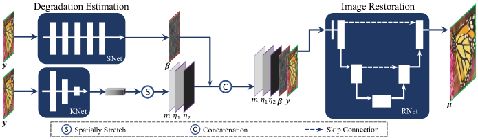
Figure 1: The inference framework of the proposed generative model for blind image super-resolution. It can be decomposed into two sub-tasks of degradation estimation and image restoration. Given any corrupted image $\bm{y}$, we firstly infer the posteriori parameters $\bm{\beta}$ of $q(\bm{\sigma}^{2}|\bm{y})$ by SNet and $\{m,\eta_{1},\eta_{2}\}$ of $q(\bm{\varLambda}|\bm{y})$ by KNet in the phase of degradation estimation, and then recover the desirable high-quality image (i.e., the mean value $\bm{\mu}$ of $q(\bm{z}|\bm{y},\bm{\sigma}^{2},\bm{\varLambda})$) by RNet under the guidance of the estimated degradation information.

3.3 Extension to Blind Super-resolution

For the problem of image super-resolution, the degradation model in Eq. (1) can be reformulated as:

$$\bm{y}=(\bm{z}*\bm{k})\downarrow_{s}+\bm{n},$$ (6)

where $\bm{k}$ denotes the blur kernel, $*$ is the convolution operator, and $\downarrow_{s}$ is the downsampler with scale factor $s$. Based on this degradation model, we extend the noise assumption of Eq. (2) as follows:

$$y_{i}\sim\mathcal{N}(y_{i}|[\bm{z}*\bm{k}]_{i},\sigma_{i}^{2}),~{}i=1,2,\cdots,d,$$ (7)

where $[\bm{z}*\bm{k}]_{i}$ represents the $i$-the pixel of $\bm{z}*\bm{k}$.

To handle blind super-resolution, the most challenging part is how to model the blur kernel. Recently, lots of related literatures [67, 68, 57, 69, 63] have found that the anisotropic Gaussian kernels are sufficient to guarantee pleasing results for image super-resolution. In this study, we follow these related works and adopt the anisotropic Gaussian kernels. Thus, the blur kernel $\bm{k}$ with size $(2r+1)\times(2r+1)$ can be defined as:

$$k_{ij} =g(\lambda_{1}^{2},\lambda_{2}^{2},\rho)$$

$$=\frac{1}{2\pi\lambda_{1}\lambda_{2}\sqrt{1-\rho^{2}}}\exp\left\{-\frac{1}{2}\bm{S}^{T}\bm{\Sigma}^{-1}\bm{S}\right\},$$ (8)

where $\bm{\Sigma}=\begin{bmatrix}\lambda_{1}^{2}&\lambda_{1}\lambda_{2}\rho\\ \lambda_{1}\lambda_{2}\rho&\lambda_{2}^{2}\\ \end{bmatrix}$ is the covariance matrix, $\rho$ is the Pearson correlation coefficient, $\bm{S}=\begin{bmatrix}i&j\\ \end{bmatrix}^{T}$ denotes the spatial coordinate with $i,j\in\{-r,\cdots,r\}$. By denoting $\bm{\varLambda}=\{\rho,\lambda_{1}^{2},\lambda_{2}^{2}\}$, one can easily observe that the blur kernel $\bm{k}$ is completely determined by $\bm{\varLambda}$ when the kernel size is fixed. This inspires us to design a prior distribution for $\bm{\varLambda}$ instead of $\bm{k}$.

In essense, Eq. (8) represents the blur kernel $\bm{k}$ through two Gaussian distributions with variance parameters $\lambda_{1}^{2}$ and $\lambda_{2}^{2}$ along the horizontal and vertical directions, and their correlations is depicted by $\rho$. For $\{\lambda_{1},\lambda_{2}\}$ and $\rho$, we impose the inverse Gamma and Dirac distributions for them as prior constraints, respectively, i.e.,

$$\bm{\varLambda}\sim p(\bm{\varLambda})=\text{Dirac}(\rho|\hat{\rho})\prod_{l=1}^{2}\text{IG}(\lambda_{l}^{2}|\kappa_{0}-1,\kappa_{0}*\hat{\lambda}_{l}^{2}),$$ (9)

where $\{\hat{\rho},\hat{\lambda}_{1}^{2},\hat{\lambda}_{2}^{2}\}$ reflect the corresponding true kernel information contained in the training data. Similar to the $\alpha_{0}$ of Eq. (4), $\kappa_{0}$ is also a hyper-parameter controlling the shape of the inverse Gamma distributions. For the purpose of easy optimization, we employ a Gaussian distribution with small variance to approximate the Dirac distribution. Thus, based on Eq. (8), the blur kernel $\bm{k}$ is modelled as:

$$\bm{k}=g(\bm{\varLambda}),$$ (10)

$$\bm{\varLambda}\sim p(\bm{\varLambda})=\mathcal{N}(\rho|\hat{\rho},r_{0}^{2})\prod_{l=1}^{2}\text{IG}(\lambda_{l}^{2}|\kappa_{0}-1,\kappa_{0}*\hat{\lambda}_{l}^{2}),$$ (11)

where the variance $r_{0}^{2}$ is empirically set as $1e\text{-}4$ throughout all our experiments.

Combining Eqs. (3)-(5), (7), and (10)-(11) (or Eqs. (2)-(5)) together, a full Bayesian model for blind image super-resolution (or image denoising) can be obtained. The goal then turns to infer the posterior of latent variables $\{\bm{z},\bm{\sigma}^{2},\bm{\varLambda}\}$ (or $\{\bm{z},\bm{\sigma}^{2}\}$) from $\bm{y}$, namely $p(\bm{z},\bm{\sigma}^{2},\bm{\varLambda}|\bm{y})$ (or $p(\bm{z},\bm{\sigma}^{2}|\bm{y})$).

4 Stochastic Variational Inference

In this section, a stochastic variational inference algorithm is designed for the proposed generative model. In the following part, we take blind super-resolution problem as an example to present our algorithm, since it can be easily degenerated into the denoising task by setting the blur kernel as Dirac delta function and the scale factor as 1.

4.1 Form of Variational Posterior

Inspired by the VI techniques [70], we firstly construct a variational distribution $q(\bm{z},\bm{\sigma}^{2},\bm{\varLambda}|\bm{y})$ to approximate the true posterior $p(\bm{z},\bm{\sigma}^{2},\bm{\varLambda}|\bm{y})$ led by our generative model. The variational posteriori distribution is then conditionally factorized as:

$$q(\bm{z},\bm{\sigma}^{2},\bm{\varLambda}|\bm{y})=q(\bm{z}|\bm{y},\bm{\sigma}^{2},\bm{\varLambda})q(\bm{\sigma}^{2}|\bm{y})q(\varLambda|\bm{y}).$$ (12)

Next, we begin to design specific forms for these three factorized posteriori distributions.

The conjugate prior of Eq. (4) inspires us to assume $q(\bm{\sigma}^{2}|\bm{y})$ as the following inverse Gamma distribution:

$$q(\bm{\sigma}^{2}|\bm{y})=\prod_{i}^{d}\text{IG}(\sigma_{i}^{2}|\alpha_{0}-1,\alpha_{0}\beta_{i}(\bm{y};W_{S})),$$ (13)

where $\beta_{i}(\bm{y};W_{S})$ is a mapping function parameterized as a DNN named as sigma network (SNet) with parameters $W_{S}$. It aims to predict the scale parameter of $q(\bm{\sigma}^{2}|\bm{y})$ directly from the corrupted image $\bm{y}$. As for the shape parameter of $q(\bm{\sigma}^{2}|\bm{y})$, we simply fix it as the same to the prior distribution, i.e., $\alpha_{0}-1$. Different from the strategy of setting them both as learnable parameters in our previous version [27], such a modification largely simplifies the evidence lower bound of Sec. 4.2 and also makes our algorithm more stable during training. Similarly, we formulate $q(\bm{\varLambda}|\bm{y})$ as:

$$q(\bm{\varLambda}|\bm{y}) =\mathcal{N}(\rho|m(\bm{y};W_{K}),r_{0}^{2})$$

$$\mathrel{\phantom{=}}\prod_{l=1}^{2}\text{IG}(\lambda_{l}^{2}|\kappa_{0}-1,\kappa_{0}\eta_{l}(\bm{y};W_{K})),$$ (14)

where $m(\bm{y};W_{K})$ and $\eta_{l}(\bm{y};W_{K})$ are jointly parameterized as a DNN with parameters $W_{K}$, named as kernel network (KNet). It takes the low-resolution image $\bm{y}$ as input and outputs the posteriori parameters for $q(\bm{\varLambda}|\bm{y})$.

As for $q(\bm{z}|\bm{y},\bm{\sigma}^{2},\bm{\varLambda})$, we set it as Gaussian distribution:

$$q(\bm{z}|\bm{y},\bm{\sigma}^{2},\bm{\varLambda})=\prod_{i}^{d}\mathcal{N}(z_{i}|\mu_{i}(\bm{y},\bm{\sigma}^{2},\bm{\varLambda};W_{R}),\varepsilon_{0}^{2}),$$ (15)

where $\mu_{i}(\bm{y},\bm{\sigma}^{2},\bm{\varLambda};W_{R})$ represents the mapping function to evaluate the mean value of the posteriori Gaussian distribution of $\bm{z}$. Naturally, it is parameterized as a DNN with parameters $W_{R}$, named as restoration network (RNet). For the ease of training, we set the variance parameter of this posteriori distribution as a constant, i.e., $\varepsilon_{0}^{2}$, being the same with that of the prior distribution in Eq. (3).

It is necessary to emphasize that the posteriori distribution $q(\bm{z}|\bm{y},\bm{\sigma}^{2},\bm{\varLambda})$ is conditioned on $\bm{\sigma}^{2}$ and $\bm{\varLambda}$, which means that RNet depends on the noise variance map estimated by SNet and the kernel informations predicted by KNet. Generally speaking, the conditional assumption of Eq. (12) decomposes the task of blind super-resolution into two cascaded sub-tasks, namely degradation estimation implemented by SNet and KNet, and non-blind image restoration implemented by RNet. The whole inference procedure is shown in Fig. 1.

Remark. In Eq. (13), the mode of $q(\bm{\sigma}^{2}|\bm{y})$ is just equal to $\bm{\beta}(\bm{y};W_{S})$, which is predicted by SNet. In other words, we leverage SNet to only estimate the core posteriori parameter, namely the mode, instead of the whole posteriori distribution. The reasons underlying this setting are two-fold. on one hand, this strategy inclines to alleviate the learning burden of SNet to some extent. On the other hand, we can directly utilize the output of SNet as an estimated variance map to solve some downstream problems that depends on pre-known noise levels. Similarly, we also employ this partially learning strategy in Eq. (14) and Eq. (15).

4.2 Evidence Lower Bound

In this part, we induce a rational objective function to jointly train the networks of SNet, KNet, and RNet. For the convenience of presentation, we simply denote $\beta_{i}(\bm{y};W_{S})$, $m(\bm{y};W_{K})$, $\eta_{l}(\bm{y};W_{K})$, and $\mu_{i}(\bm{y},\bm{\sigma}^{2},\bm{\varLambda};W_{R})$ as $\beta_{i}$, $m$, $\eta_{l}$, and $\mu_{i}$ respectively. Given any corrupted image $\bm{y}$, its logarithm marginal probability can be decomposed as

$$\log p(\bm{y}) =\mathcal{L}(\bm{z},\bm{\sigma},\bm{\varLambda};\bm{y})$$

$$\mathrel{\phantom{=}}+KL\Big{[}q(\bm{z},\bm{\sigma}^{2},\bm{\varLambda}|\bm{y})\|p(\bm{z},\bm{\sigma}^{2},\bm{\varLambda}|\bm{y})\Big{]},$$ (16)

where

$$\mathcal{L}(\bm{z},\bm{\sigma},\bm{\varLambda};\bm{y}) =E_{q}\Big{[}\log p(\bm{y}|\bm{z},\bm{\sigma}^{2},\bm{\varLambda})p(\bm{z})p(\bm{\sigma}^{2})p(\bm{\varLambda})$$

$$\mathrel{\phantom{=}}-\log q(\bm{z},\bm{\sigma}^{2},\bm{\varLambda}|\bm{y})\Big{]}.$$ (17)

Here $E_{q}[\cdot]$ denotes the expectation w.r.t. the posteriori distribution $q(\bm{z},\bm{\sigma}^{2},\bm{\varLambda}|\bm{y})$. The second term of Eq. (16) represents the KL divergence between the variational posterior $q(\bm{z},\bm{\sigma}^{2},\bm{\varLambda}|\bm{y})$ and the true posterior $p(\bm{z},\bm{\sigma}^{2},\bm{\varLambda}|\bm{y})$. Due to the non-negtiveness of KL divergence, $\mathcal{L}(\bm{z},\bm{\sigma},\bm{\varLambda};\bm{y})$ constitutes a lower bound of $\log p(\bm{y})$, generally called evidence lower bound (ELBO). Therefore, we can naturally approximate the true posteriori $p(\bm{z},\bm{\sigma}^{2},\bm{\varLambda}|\bm{y})$ with $q(\bm{z},\bm{\sigma}^{2},\bm{\varLambda}|\bm{y})$ through maximizing the ELBO.

Combining the factorized assumption of Eq. (12), the ELBO can be rewritten as

$$\mathcal{L}(\bm{z},\bm{\sigma},\bm{\varLambda};\bm{y}) =E_{q(\bm{z},\bm{\sigma},\bm{\varLambda}|\bm{y})}\Big{[}\log p(\bm{y}|\bm{z},\bm{\sigma}^{2},\bm{\varLambda})\Big{]}$$

$$-E_{q(\bm{\sigma},\bm{\varLambda}|\bm{y})}\Big{[}KL\left[q(\bm{z}|\bm{y},\bm{\sigma}^{2},\bm{\varLambda})\|p(\bm{z})\right]\Big{]}$$

$$-KL\Big{[}q(\bm{\sigma}^{2}|\bm{y})\|p(\bm{\sigma}^{2})\Big{]}$$

$$-KL\Big{[}q(\bm{\varLambda}|\bm{y})\|p(\bm{\varLambda})\Big{]},$$ (18)

where $q(\bm{\sigma},\bm{\varLambda}|\bm{y})=q(\bm{\sigma}|\bm{y})q(\bm{\varLambda}|\bm{y})$.

Next, we consider how to calculate each term in Eq. (18) step by step. The first term is intractable, mainly because the posterior $q(\bm{z},\bm{\sigma},\bm{\varLambda}|\bm{y})$ is parameterized as complicated forms of DNNs. Fortunately, we can use the reparameterization trick [71] to obtain multiple differentiable samples from the posteriors, and then use them to estimate these two terms by Monte Carlo (MC) like VAE [71]. Concretely, the re-sampling process from $q(\bm{z}|\bm{y},\bm{\sigma}^{2},\bm{\varLambda})$ can be easily implemented as

$$\bm{\tilde{z}}=\bm{\mu}+\varepsilon_{0}\bm{\tau},~{}\bm{\tau}\sim\mathcal{N}(\tau|\bm{0},I).$$ (19)

To sample from $q(\bm{\varLambda}|\bm{y})$ and $q(\bm{\sigma}^{2}|\bm{y})$, we adopt the pathwise derivative technology [72] and denote the re-sampled data example as $\tilde{\bm{\varLambda}}$ and $\tilde{\bm{\sigma}}^{2}$. Based on $\tilde{\bm{z}}$, $\tilde{\bm{\varLambda}}$ and $\tilde{\bm{\sigma}}^{2}$, the first term of Eq. (18) can be approximated as follows:

$$\mathrel{\phantom{\approx}}E_{q(\bm{z},\bm{\sigma},\bm{\varLambda}|\bm{y})}\left[\log p(\bm{y}|\bm{z},\bm{\sigma}^{2},\bm{\varLambda})\right]$$

$$\approx-\frac{1}{2}\sum_{i=1}^{d}\Big{\{}\log\tilde{\sigma}_{i}+w_{i}\left(y_{i}-[\tilde{\bm{z}}*\tilde{\bm{k}}]_{i}\right)^{2}\Big{\}},$$ (20)

where $w_{i}=\frac{1}{\tilde{\sigma}_{i}^{2}}$, $\tilde{\bm{k}}=g(\tilde{\bm{\varLambda}})$, and $g(\cdot)$ is defined in Eq. (10). Note that we have omitted a constant that is independent of the learnable parameters in Eq. (20).

As for the last three terms of Eq. (18), they can all be analytically calculated as follows:

$$E_{q(\bm{\sigma},\bm{\varLambda}|\bm{y})}\Big{[}KL\left[q(\bm{z}|\bm{y},\bm{\sigma}^{2},\bm{\varLambda})\|p(\bm{z})\right]\Big{]}=\sum_{i=1}^{d}\frac{(\mu_{i}-x_{i})^{2}}{2\varepsilon_{0}^{2}},$$ (21)

$$KL\Big{[}q(\bm{\sigma}^{2}|\bm{y})\|p(\bm{\sigma}^{2})\Big{]}=\sum_{i=1}^{d}\alpha_{0}\left(\frac{\xi_{i}}{\beta_{i}}+\log\frac{\beta_{i}}{\xi_{i}}-1\right),$$ (22)

$$KL\Big{[}q(\bm{\varLambda}|\bm{y})\|p(\bm{\varLambda})\Big{]}=\frac{(m-\hat{\rho})^{2}}{2r_{0}^{2}}+\sum_{l=1}^{2}\kappa_{0}\left(\frac{\hat{\lambda}_{l}}{\eta_{l}}+\log\frac{\eta_{l}}{\hat{\lambda}_{i}}-1\right).$$ (23)

Finally we can get the expected objective function, namely the negative ELBO on the entire training dataset, to optimize the network parameters of $W_{S}$, $W_{K}$, and $W_{R}$ as follows:

$$\min_{W_{S},W_{K},W_{R}}-\sum_{j=1}^{N}\mathcal{L}(\bm{z}^{(j)},\bm{\sigma}^{(j)},\bm{\varLambda}^{(j)};\bm{y}^{(j)}),$$ (24)

where $\bm{z}^{(j)}$, $\bm{\sigma}^{(j)}$, and $\bm{\varLambda}^{(j)}$ denote the posteriori parameters for the $j$-th image pair in training dataset $\mathcal{D}$.

With the negative ELBO loss in Eq. (24), it is easy to train our model in an end-to-end manner like the DL-based methods. Actually, each term of the ELBO can be intuitively explained: the last three terms of KL divergence in Eq. (18) control the discrepancy between the variational posteriors and the priors, and the first term is the likelihood of the observed low-resolution images in the training dataset, which enforces the recovered high-resolution image can be mapped back to the low-resolution one through the estimated degradation model. During training, SNet, KNet, and RNet are refined and guided by each other under the supervision of this loss function.

Remark. Most of the current IR methods assume that each element of the data fidelity (i.e., the likelihood) term is with the same importance, i.e., $\sum_{i}\left(y_{i}-[\tilde{\bm{z}}*\tilde{k}]_{i}\right)^{p}$. In this work, we novelly exploit an adaptive manner to re-weight the data fidelity in terms of $l_{2}$-norm, i.e., $\sum_{i}w_{i}\left(y_{i}-[\tilde{\bm{z}}*\tilde{k}]_{i}\right)^{2}$ in Eq. (20). Each pixel is re-weighted by $w_{i}=\frac{1}{\tilde{\sigma}_{i}^{2}}$, in which $\tilde{\sigma}_{i}^{2}$ is sampled from the noise distribution estimated by SNet. This re-weighting strategy based on noise variance is generally used in Bayesian statistics, like in [11, 13].

TABLE I: The PSNR and SSIM results of different methods on three groups of testing datasets. The best and second best results are highlighted in bold and underline, respectively. Note that * denotes non-blind methods that rely on the pre-given noise-level.

Cases	Datasets	Metrics	Methods
11
			NLM [3]	CBM3D [4]	DnCNN [17]	FFDNet∗ [20]	S2S [73]	Ne2Ne [74]	DRUNet∗ [50]	VIRNet
Case 1	CBSD68	PSNR	24.06	26.73	28.74	28.79	28.23	27.92	29.05	29.28
		SSIM	0.6190	0.7660	0.8181	0.8181	0.7968	0.7948	0.8349	0.8353
11
	McMaster	PSNR	25.08	27.47	29.49	30.17	29.87	29.63	30.86	31.00
		SSIM	0.6910	0.7800	0.8218	0.8394	0.8374	0.8263	0.8640	0.8642
Case 2	CBSD68	PSNR	22.40	25.42	28.15	28.42	27.87	25.26	28.64	28.93
		SSIM	0.5582	0.7040	0.7989	0.8079	0.7859	0.6870	0.8251	0.8269
11
	McMaster	PSNR	23.26	25.82	28.84	29.74	29.43	27.23	30.38	30.58
		SSIM	0.6126	0.7120	0.7994	0.8315	0.8284	0.7314	0.8545	0.8572
Case 3	CBSD68	PSNR	24.07	26.85	28.64	28.68	28.14	27.33	29.12	29.19
		SSIM	0.6153	0.7360	0.8143	0.8141	0.7931	0.7629	0.8321	0.8323
11
	McMaster	PSNR	25.13	27.62	29.36	30.02	29.75	28.97	30.82	30.85
		SSIM	0.6845	0.7520	0.8184	0.8365	0.8354	0.7982	0.8610	0.8612

4.3 Network Structure and Learning

As shown in Fig. 1, SNet takes the corrupted image $\bm{y}$ as input and outputs the scale-related parameter of $q(\bm{\sigma}^{2}|\bm{y})$, achieving the goal of noise estimation. In practice, it consists of five convolutional layers, and each is followed with a Leaky ReLU activation except for the first and last layers. As for the KNet, it is designed to predict the posteriori distribution of the kernel parameter $\bm{\varLambda}$ from the corrupted image $\bm{y}$. In implementation, we firstly employ one convolutional layer and eight channel attention blocks (CAB) [23] to extract abundant feature maps, and then fuses them by one convolutional layer followed by an average pooling layer to obtain the posteriori parameters in $q(\bm{\varLambda}|\bm{y})$.

The design of RNet, aiming to infer the conditional posteriori distribution of the desirable high-quality image, plays the most important role in blind IR. We adopt the commonly used ResUNet [56, 54] in low-level vision as our backbone. It replaces the plain convolutional layer in UNet [75] with residual block [76], and thus makes the gradient flow propagate much faster. Furthermore, in purpose of leveraging the estimated noise and kernel informations by SNet and KNet, we concatenate their outputs with the corrupted image $\bm{y}$ together (see Fig. 1), and then feed them into RNet to recover the high-resolution image. We empirically find that such a simple concatenated operation performs very well and stably in our inference framework.

It should be noted that this work does not aim to design more effective network architectures to surpass current SotA methods, but mainly focus on devising a probabilistic framework based on the deep variational inference to deal with the blind IR task. Therefore, we simply select the commonly used networks in low-level vision as our backbones for SNet, KNet, and RNet, so as to better verify the generality of the proposed model.

5 Experimental Results

In this section, we evaluate the effectiveness of our proposed method on two typical IR tasks, namely image denoising and image super-resolution. We denote our Variational Image Restoration Network as VIRNet for notation convenience in the following presentation.

To optimize the network, we adopted the Adam [77] algorithm with a mini-batch size of 16 and other default settings of PyTorch [78]. The initial learning rate was set as $10^{-4}$ and decayed gradually using the consine annealing strategy [79]. For computational stability, the gradient clipping strategy was also used during training. In the task of image denoising, we cropped small image patches with a size of $128\times 128$ for training. The hyper-parameter $\varepsilon_{0}^{2}$ of Eq. (3) was set to be $10^{-6}$, and the window size $p$ of Eq. (5) was set to be $7$. In the task of image super-resolution, the patch size during training was fixed as $96$, $144$, and $192$ for scale factor 2, 3, and 4 respectively. The hyper-parameter $\varepsilon_{0}^{2}$ was set to be $10^{-5}$, while the window size $p$ was set as a larger value $11$ than that in denoising, since image noise in super-resolution is usually assumed to be i.i.d. Gaussian. As for the shape parameter $\kappa_{0}$ of the kernel prior distribution in Eq. (11), we empirically set it as 50.

5.1 Image Denoising Experiments

5.1.1 Synthetic Non-I.I.D. Gaussian Noise Removal

To verify the effectiveness and robustness of VIRNet under non-i.i.d. noise configurations, we synthesized a large set of noisy/clean image pairs as training data. Similar to [20], a set of high quality source images was firstly collected as clean ones, including 432 images from BSD500 [80], 400 images from the ImageNet [81] validation set and 4744 images from Waterloo Database [82]. We then randomly generated non-i.i.d. Gaussian noise as

$$\bm{n}=\bm{n}^{1}\odot\bm{M},~{}\bm{n}^{1}\sim\mathcal{N}(\bm{n}^{1}|\bm{0},\bm{I}),$$ (25)

where $\bm{I}$ is identity matrix, $\bm{M}$ is a spatially variant map with the same size as the source image. Finally, the noisy image was obtained by adding the generated noise $\bm{n}$ to the source image. As for the testing images, two commonly-used datasets, i.e., BSD68 [80] and McMaster [83], were adopted to evaluate the performance of different methods. Note that we totally generated four kinds of $\bm{M}$s as shown in Fig. 2. The first one (Fig. 2 (a)) was used for generating noisy images in training data, and the others (Fig. 2 (b1)-(d1)) for three groups of testing data (denoted as Cases 1-3). Under these settings, the noise in training data and testing data are evidently different, which is suitable to verify the generalization capability of VIRNet.

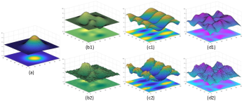
Figure 2: (a) The spatially variant map $\bm{M}$ for noise generation in training data. (b1)-(d1): Three different $\bm{M}$s on testing data in Cases 1-3. (b2)-(d2): Predicted $\bm{M}$s by our method on testing data.

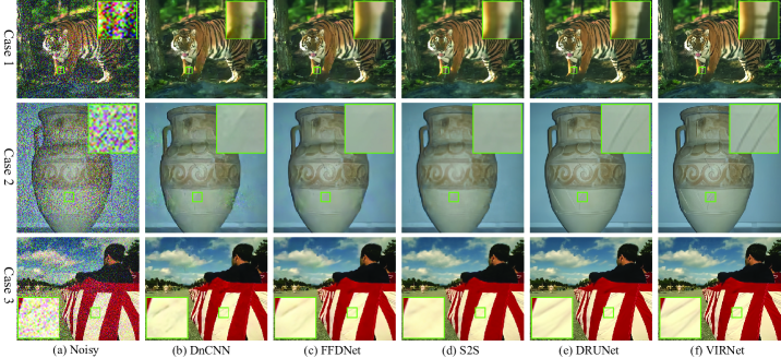
Figure 3: Denoising results of different competing methods on three typical test examples of synthetic non-i.i.d. Gaussian Noise Removal.

TABLE II: The PSNR/SSIM results of different methods under AWGN noises. The best and second best results are highlighted in bold and underlinse, respectively. Note that * denotes non-blind methods that rely on the pre-given noise level.

Cases	Datasets	Metrics	Methods
11
			CBM3D [4]	DnCNN [17]	FFDNet∗ [20]	S2S [73]	Ne2Ne [74]	RNAN∗ [21]	DRUNet∗ [50]	VIRNet
$\sigma=15$	CBSD68	PSNR	33.56	33.88	33.87	32.16	33.55	-	34.18	34.27
		SSIM	0.9237	0.9288	0.9288	0.9026	0.9262	-	0.9341	0.9340
11
	McMaster	PSNR	34.05	33.45	34.65	33.20	34.49	-	35.33	35.33
		SSIM	0.9105	0.9034	0.9214	0.9014	0.9208	-	0.9323	0.9312
$\sigma=25$	CBSD68	PSNR	30.81	31.22	31.20	30.22	31.07	-	31.50	31.65
		SSIM	0.8700	0.8824	0.8817	0.8563	0.8815	-	0.8917	0.8918
11
	McMaster	PSNR	31.68	31.50	32.34	31.56	32.27	-	33.02	33.08
		SSIM	0.8700	0.8691	0.8857	0.8745	0.8876	-	0.9028	0.9017
$\sigma=50$	CBSD68	PSNR	27.47	27.91	27.95	27.58	27.83	28.25	28.15	28.45
		SSIM	0.7680	0.7885	0.7882	0.7716	0.7829	0.8010	0.8082	0.8092
11
	McMaster	PSNR	28.53	28.61	29.17	29.11	29.10	29.69	29.84	30.02
		SSIM	0.7894	0.7984	0.8138	0.8191	0.8147	0.8326	0.8445	0.8433

TABLE III: Comparison results with current DL-based methods on model parameters (in M) and FLOPs (in G).

Metrics	Methods
6
	DnCNN	FFDNet	RNAN	DRUNet	VIRNet
# Param	0.67	0.85	8.96	32.64	10.54
FLOPs	175	56	3420	574	680

Comparison with the SotAs. We compare VIRNet with several current denoising methods, including two typical model-based methods NLM [3] and CBM3D [4], two deep self-supervised methods S2S [73] and Ne2Ne [74], three supervised learning-based methods, namely DnCNN [17], FFDNet [20], and DRUNet [54]. The PSNR and SSIM results of all comparison methods on three groups of testing data are listed in Table I. We can easily see that: 1) the proposed VIRNet outperforms the other methods in all cases, indicating its superiority on handling these complicated non-i.i.d. noise types; 2) on the whole, DL-based methods (including the self-supervised methods) evidently surpass classical model-based methods NLM and CBM3D, owning to the powerful non-linear fitting capability of DNNs; 3) FFDNet and DRUNet are both non-blind methods that rely on the pre-given noise level as input. In contrast, VIRNet is designed toward blind IR, and thus able to simultaneously infer the noise distribution and remove the noise. Even so, VIRNet still achieves obvious performance improvements compared with FFDNet and DRUNet. This indicates the effectiveness of the Bayesian generative model and the variational inference framework.

Fig. 3 shows the visual results of different methods under testing cases 1-3 of Table I. Note that we only display the best five DL-based methods due to page limitation. It can be easily seen that the comparison methods are able to remove most of the noises, but also often generate over-smooth and blurry recovery, especially in the heavy-noise areas. This can be explained by the fact that they do not consider the spatial noise variations. To handle such non-i.i.d. noise, the proposed VIRNet elaborately considers the noise configurations and is thus capable of preserving more image details (e.g., edges, structures) than other methods.

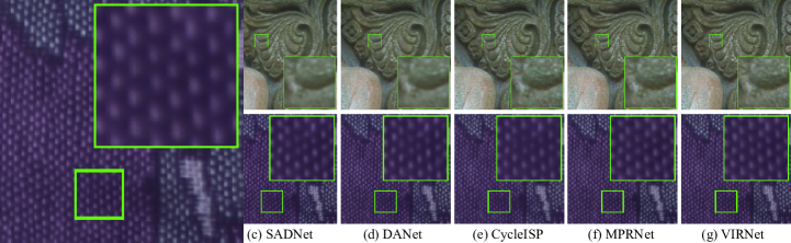
Figure 4: Denoising results of all competing methods on two typical real-world examples from DND [84] (upper) and SIDD [65] (lower) datasets.

Even though our VIRNet is designed and trained on the non-i.i.d. noise settings, it also performs well in additive white Gaussian noise (AWGN) removal tasks. Table II lists the average PSNR and SSIM results of different methods under three noise levels (i.e., $\sigma$=15, 25, 50) of AWGN. In this part, we further add the method RNAN [21] for a more thorough evaluation. It is noteworthy that RNAN is separately trained on some specific noise levels for AWGN, and hence we can only compared with it on the noise level 50. It is easy to see that VIRNet obtains the best (8 out of 12 cases) or at least second best (4 out of 12 cases) performance compared with these comparison methods. Combining the results in Table I and Table II, it should be rational to say that the proposed VIRNet is more robust. Specifically, it is hopeful to handle a wider range of noise types, due to its more flexible noise modeling essence.

In Table III, we further list the comparison results on the number of model parameters and FLOPs with four DL-based methods. The FLOPs listed in this table are calculated on images with a size of $512\times 512$. It should be noted that, for the sake of fair comparisons, the self-supervised methods S2S [73] and Ne2Ne [74] are not reported in Table III. It can be easily observed that VIRNet exhibits a better compromise over current SotA methods RNAN [21] and DRUNet [46] when taking both the model parameters and FLOPs into consideration. The proposed VIRNet is thus expected with better practical applicability in real scenarios.

5.1.2 Real-world Noise Removal

In this part, we evaluate the performance of VIRNet on two widely used real-world benchmark datasets, namely DND [84] and SIDD [65]. DND consists of 50 high-resolution images with realistic noise from 50 scenes taken by 4 consumer cameras, but it does not provide any other noisy/clean image pairs as training data. SIDD is another real-world denoising benchmark, containing about 30,000 real noisy images captured by 5 cameras under 10 scenes. Different from DND, each noisy image in SIDD comes with an almost noise-free counterpart as groundtruth, which is estimated by some statistical methods [65]. Further, SIDD also provides a small version dataset containing 320 image pairs, called SIDD-Medium, which is commonly-used as training data in recent works [27, 23, 24]. In order to compare with them fairly, we also train VIRNet only based on the SIDD-Medium dataset. As for the metrics, we adopt PSNR and SSIM [85] calculated on the sRGB space to quantitatively evaluate different methods.

TABLE IV: Comparisons of different methods in terms of denoising performance, the number of model parameters (in M), FLOPs (in G), and running time (in seconds). Note that PNGAN follows the same network architecture and the training strategy with MPRNet, and further improves the performance by simulating more training data. Thus we mark its results with gray color to denote unfair comparisons.

Methods	SIDD		DND		Model Profile
8
	PSNR	SSIM	PSNR	SSIM	# Param	FLOPs	Time
CBM3D [4]	25.65	0.685	34.51	0.851	-	-	21.49
DnCNN [17]	23.66	0.583	32.43	0.790	0.67	175	0.22
CBDNet [22]	30.78	0.801	38.06	0.942	4.37	161	0.19
RIDNet [23]	38.71	0.951	39.26	0.953	1.5	393	0.68
AINDNet [86]	38.95	0.952	39.37	0.951	13.76	1284	0.49
VDN [27]	39.23	0.955	39.38	0.952	7.81	168	0.20
SADNet [87]	39.46	0.957	39.59	0.952	4.23	76	0.22
DANet [24]	39.47	0.957	39.58	0.955	9.15	59	0.12
CycleISP [88]	39.52	0.957	39.56	0.956	2.83	739	1.36
MPRNet [25]	39.62	0.958	39.80	0.954	15.74	2296	2.75
VIRNet (Ours)	39.64	0.958	39.83	0.954	15.40	658	0.88
PNGAN [89]	40.06	0.960	40.25	0.962	15.74	2296	2.75

We compared VIRNet with several typical real-world denoising methods, including MPRNet [25], CycleISP [88], DANet [24], SADNet [87], VDN [27] and so on (see Table IV). To the best of our knowledge, current SotA method on this two benchmarks is PNGAN [89]. This work, however, mainly focuses on simulating the camera pipeline to generate large amount of image pairs as training data so as to further improve the performance, instead of designing more effective denoising algorithm. Its denoiser architecture and the training strategy completely follow MPRNet. Therefore we mainly compare with MPRNet in this work.

In order to comprehensively evaluate all competing methods, Table IV lists the denoising performance, as well as the model profiles, including the number of network parameters, the FLOPs, and the feedforward running time of the denoisers. The FLOPs and running time are both counted on images with a size of $512\times 512$. From the perspective of denoising performance, the proposed VIRNet achieves a slight performance improvements compared with current SotA method MPRNet, indicating its effectiveness. However, VIRNet is with pronounced superiorities in terms of model profiles, especially in the comparisons of FLOPs and running time, which more faithfully reflect the relative efficiency of our method. To intuitively compare the denoising results, we visualize two typical real examples in Fig. 4, which are consistent with the quantitative results in Table IV.

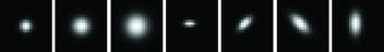
Figure 5: Seven Gaussian kernels used to generate the LR images in the synthetical super-resolution experiments.

TABLE V: Quantitative comparisons of different methods under a scale factor of 4. The PSNR/SSIM/LPIPS values in this table are all averaged over the seven kernels as shown in Fig. 5. The results of the non-blind methods that rely on the pre-given groundtruth blur kernel and noise level are marked in gray color to denote unfair comparisons. Besides, some commonly considered model profiles, namely, the number of learnable parameters (in M), the FLOPs (in G), and the running time (in seconds), are also listed for more comprehensive comparison. Note that the FLOPs and running time are calculated in the case of super-resolving the low-resolution images with a size of $256\times 256$.

Methods	Noise Level	Set14			CBSD68			DIV2K100			Model Profile
14
		PSNR$\uparrow$	SSIM$\uparrow$	LPIPS$\downarrow$	PSNR$\uparrow$	SSIM$\uparrow$	LPIPS$\downarrow$	PSNR$\uparrow$	SSIM$\uparrow$	LPIPS$\downarrow$	# Param	FLOPs	Times
Bicubic	0	24.54	0.6352	0.5257	24.68	0.6144	0.6044	25.50	0.6762	0.5349	-	-	0.006
HAN [90]		25.36	0.6731	0.4693	25.35	0.6494	0.5477	26.30	0.7115	0.4775	16.07	4653	4.933
IKC [44]		27.24	0.7388	0.3534	26.70	0.7105	0.4253	28.00	0.7741	0.3517	9.05	11537	7.392
DAN [57]		27.49	0.7464	0.3442	26.96	0.7204	0.4053	28.31	0.7832	0.3354	4.33	5013	2.012
DASR [69]		27.74	0.7512	0.3314	27.12	0.7231	0.4026	28.32	0.7805	0.3380	7.25	839	0.525
BSRNet [46]		26.84	0.7129	0.3819	26.38	0.6860	0.4540	27.49	0.7503	0.3829	16.70	4706	1.557
VIRNet (Ours)		27.89	0.7573	0.3165	27.27	0.7330	0.3868	28.60	0.7919	0.3165	5.72	370	0.161
14
GT+SRMD [68]		27.83	0.7587	0.3180	27.12	0.7283	0.3962	28.44	0.7874	0.3250	1.55	407	0.106
GT+USRNet [56]		27.90	0.7747	0.3181	26.88	0.7408	0.3988	28.84	0.8086	0.3042	17.20	38893	9.214
Bicubic	2.55	24.51	0.6314	0.5590	24.67	0.6114	0.6332	25.44	0.6713	0.5777	-	-	0.006
DnCNN [17]+HAN [90]		25.24	0.6596	0.5213	25.23	0.6350	0.6024	26.11	0.6925	0.5618	16.07	4653	4.933
DnCNN [17]+IKC [44]		25.80	0.6795	0.4590	25.66	0.6546	0.5297	26.59	0.7144	0.4702	9.05	11537	7.392
DnCNN [17]+DAN [57]		25.43	0.6685	0.4873	25.46	0.6475	0.5524	26.32	0.7062	0.4964	4.33	5013	2.012
DASR [69]		27.05	0.7197	0.3672	26.50	0.6881	0.4479	27.58	0.7491	0.3830	7.25	839	0.525
BSRNet [46]		26.70	0.7093	0.3801	26.23	0.6797	0.4562	27.31	0.7431	0.3858	16.70	4706	1.557
VIRNet (Ours)		27.18	0.7255	0.3524	26.63	0.6975	0.4305	27.86	0.7597	0.3588	5.72	370	0.161
14
GT+SRMD [68]		27.15	0.7270	0.3549	26.54	0.6954	0.4367	27.76	0.7578	0.3647	1.55	407	0.106
GT+USRNet [56]		27.42	0.7484	0.3395	26.53	0.7125	0.4249	28.27	0.7809	0.3366	17.20	38893	9.214
Bicubic	7.65	24.25	0.6051	0.6749	24.38	0.5836	0.7662	25.08	0.6381	0.7460	-	-	0.006
DnCNN [17]+HAN [90]		24.30	0.5623	0.6899	24.24	0.5321	0.7934	24.78	0.5613	0.7837	16.07	4653	4.933
DnCNN [17]+IKC [44]		25.37	0.6566	0.4639	25.28	0.6323	0.5351	26.13	0.6935	0.4738	9.05	11537	7.392
DnCNN [17]+DAN [57]		25.05	0.6474	0.4991	25.12	0.6253	0.5702	25.97	0.6869	0.5094	4.33	5013	2.012
DASR [69]		26.19	0.6845	0.4055	25.75	0.6516	0.4935	26.75	0.7165	0.4229	7.25	839	0.525
BSRNet [46]		25.58	0.6703	0.4195	25.20	0.6385	0.5083	26.08	0.7023	0.4442	16.70	4706	1.557
VIRNet (Ours)		26.22	0.6873	0.3973	25.81	0.6576	0.4830	26.91	0.7227	0.4103	5.72	370	0.161
14
GT+SRMD [68]		26.20	0.6881	0.3999	25.74	0.6556	0.4893	26.83	0.7212	0.4156	1.55	407	0.106
GT+USRNet [56]		26.81	0.7115	0.3705	26.09	0.6745	0.4616	27.43	0.7440	0.3818	17.20	38893	9.214

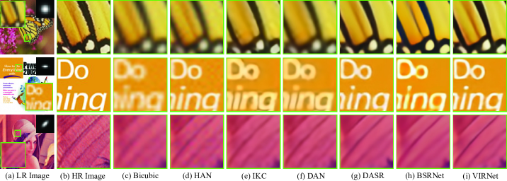
Figure 6: Visualized super-resolution results of different methods on a synthetic example of Set14 [91] under a scale factor of 4. Specifically, the noise level is 2.55, and the blur kernel is shown on the upper-right corner of the LR image.

5.2 Image Super-resolution Experiments

In this section, we apply our proposed VIRNet to blind image super-resolution. Following [69], the DF2K dataset (containing 800 images from DIV2K [92] and 2650 images from Flickr2K [93]) was employed as our training data. When synthesizing the LR images, we followed the settings of current blind SR literatures [57, 69], i.e.,

$$\bm{y}=(\bm{z}\otimes\bm{k})\downarrow_{s}^{d}+\bm{n},$$ (26)

where $\bm{y}$ and $\bm{z}$ denote the low-resolution and high-resolution image respectively, $\otimes$ is the 2-D convolution, $\downarrow_{s}^{d}$ is the direct downsampler with a scale factor of $s$, and $\bm{n}$ is the i.i.d. Gaussian noise with noise level $\sigma$. For blur kernel $\bm{k}$, we adopted the general anisotropic Gaussian kernel with a size of $21\times 21$, and its covariance matrix $\bm{\Sigma}$ was generated as [94], i.e.,

$$\bm{U}=\begin{bmatrix}\cos{\theta}&-\sin{\theta}\\ \sin{\theta}&\cos{\theta}\end{bmatrix},~{}\bm{\Lambda}=\begin{bmatrix}l_{1}^{2}&0\\ 0&l_{2}^{2}\end{bmatrix},~{}\bm{\Sigma}=\bm{U}\bm{\Lambda}\bm{U}^{T}.$$ (27)

To be specific, $l_{1}$, $l_{2}$, and $\theta$ are randomly sampled from $[0,s]$, $[0,s]$, and $[0,\pi]$ respectively. For the noise level $\sigma$, we set its range to be $[0,15]$.

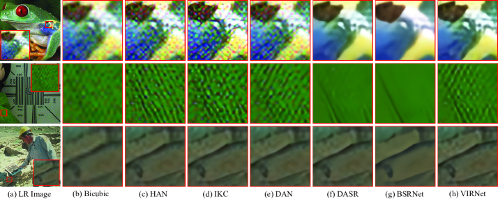
Figure 7: Visualized super-resolution results of different methods on three examples of RealSRSet [46] under a scale factor of 4.

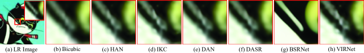
Figure 8: One typical super-resolution result on an example from RealSRSet [46] with a scale factor of 4. In this example, most of the methods fail to obtain one high-quality HR image except for BSRNet, mainly owning to their mismatch on image degradation.

5.2.1 Results on Synthetic Data

To be capable of quantitatively evaluating different methods, we firstly conducted some synthetical experiments on three commonly used datasets, including Set14 [91], CBSD68 [80], and DIV2K100 (the validation set of DIV2K [92]). For the purpose of making a thorough comparison on various degradations, we considered seven representive and diverse kernels as shown in Fig. 5, including three isotropic Gaussian kernels with different kernel widths (i.e., 0.4$s$, 0.6$s$, and 0.8$s$) and four anisotropic Gaussian kernels, where $s$ is the scale factor. In addition, three noise levels (i.e., $0$, $2.55$, and $7.65$) are considered following [56]. As for the metrics, aside from the commonly used PSNR and SSIM [85], we also adopted LPIPS [95] to measure the preceptual similarity. Note that PSNR and SSIM are calculated on the Y channel of the YCbCr space, while LPIPS is calculated in the sRGB space.

TABLE VI: The non-reference comparison results of different methods on the real-world dataset SRRealSet [46] under a scale factor of 4. Best and second best results are highlighted by bold and underline, respectively.

Metrics	Methods
8
	Bicubic	HAN	IKC	DAN	DASR	BSRNet	VIRNet
NRQM$\uparrow$	3.35	4.53	4.72	4.43	4.18	4.30	4.68
PI$\downarrow$	6.36	5.55	5.33	5.54	5.73	5.50	5.39

We consider three categories of comparison methods: 1) classical Bicubic interpolation method; 2) five blind super-resolution methods, including HAN [90], IKC [44], DAN [57], DASR [69], and BSRNet [46]; 3) two non-blind methods, i.e., SRMD [68] and USRNet [56], which rely on the pre-given blur kernel and noise level as input. For these non-blind methods, we provided the groundtruth blur kernel and noise level for them, and denoted their results with the format of “GT+X” (e.g., GT+SRMD). In addition, for the methods of HAN, IKC and DAN, we firstly denoised the noisy low-resolution image using DnCNN [17] and then super-resolved it in the cases of $\sigma=\{2.55,7.65\}$, since these methods do not consider image noise during training.

Table V lists the comparison results of different methods under a scale factor of 4, and more results under scale factors of 2 and 3 are put into the supplementary material. From Table V, it can be seen that the proposed VIRNet achieves the best performance among blind methods in all cases. Especially, compared with the non-blind methods, VIRNet is still able to obtain a slightly better or at least comparable results even though they make use of the groudtruth information of blur kernel and noise level. This indicates the effectiveness of the proposed blind framework which is capable of handling the tasks of degradation estimation and image restoration simultaneously. Further, taking the model profiles into consideration, the superiorities of VIRNet is more evident. Specifically, VIRNet has fewer number of parameters, fewer FLOPs, and faster speed than both the SotA blind method DASR [69] and the non-blind method USRNet [56].

In Fig. 6, we display the denoising results on three typical visual examples of Set14 with a scale factor of 4. Note that we only show the results of blind super-resolution methods for a fair comparison. It can be easily seen that the proposed VIRNet is able to recover more realistic and sharper results, which are evidently closer to the groudtruth high-resolution images than other methods. The results of most comparison methods are relatively blurry and lose some image details. In the second example (the middle row), IKC and DAN lead to a relatively severe corruption on the original image color. That’s possibly caused by the inconsistency of their multiple iterations, since they both adopt the coarse-to-fine manner to gradually adjust the results. Due to the careful considerations on the degradation model, DASR and BSRNet also perform well compared with other methods. However, VIRNet still evidently surpasses them in terms of the quantitative and qualitative results. This further substantiates the effectiveness of the proposed variational framework.

TABLE VII: The PSNR results of FFDNet [20] with the groudtruth noise level and with that estimated by the proposed VIRNet on CBSD68 [80] under the i.i.d. Gaussian noise setting.

Methods	Noise Levels
4
	$\sigma=15$	$\sigma=25$	$\sigma=50$
$\text{FFDNet}_{\text{GT}}$	33.87	31.20	27.95
$\text{FFDNet}_{\text{VIR}}$	33.87	31.20	27.92

TABLE VIII: The PSNR results of FFDNet [20] with the groudtruth noise variance map and with that estimated by the proposed VIRNet on CBSD68 [80] under the non-i.i.d. Gaussian noise.

Methods	Noise Cases
4
	Case 1	Case 2	Case 3
$\text{FFDNet}_{\text{GT}}$	28.79	28.42	28.68
$\text{FFDNet}_{\text{VIR}}$	28.75	28.39	28.65

TABLE IX: The average kernel MSE (1E-5) values of different methods on DIV2K20 with a scale factor of 4.

Metrics	Methods
5
	KernelGan [96]	DIPFKP [63]	BSRDM [64]	VIRNet
MSE$\downarrow$	4.34	1.73	1.60	0.89

5.2.2 Results on Real Data

In this part, we further justify the effectiveness of the proposed VIRNet on the real-world dataset RealSRSet [46]. It contains 20 real images that are commonly used in previous literatures [97, 98, 99, 20] or downloaded from internet. Since the underlying high-resolution images for them are not available, we thus mainly evaluate different methods by visual comparisons. Fig. 7 displays three typical super-resolution examples with a scale factor of 4. In the first (top row) and second (middle row) examples, the LR images both contain some image noises, which makes the super-resolution goal more challenging. The methods of Bicubic, HAN, IKC, and DAN all fail to deal with such cases, and produce some artifacts in the areas with image noises. As for DASR and BSRNet, they unfortunately erase the high frequency image details when removing the image noises. One can easily observe that the proposed VIRNet makes a good trade-off between preserving the image details and removing the image noises. In the third (bottom row) example, the results of IKC and VIRNet are more natural and realistic than others that are all blurry to different extent. These results verify the stable and consistently well performance of VIRNet in the real-world super-resolution task.

TABLE X: The average comparison results of USRNet combined with different kernel estimation methods on DIV2K20 with a scale factor of 4. Note that “GT+USRNet” denotes the results of USRNet with the pre-given groudtruth kernels.

Methods	Metrics
4
	PSNR$\uparrow$	SSIM$\uparrow$	LPIPS$\downarrow$
KernelGan [96]+USRNet [56]	14.52	0.358	0.522
DIPFKP [63]+USRNet [56]	24.02	0.676	0.363
BSRDM [64]+USRNet [56]	27.07	0.771	0.326
VIRNet+USRNet [56]	28.53	0.796	0.313
GT+USRNet [56]	29.19	0.805	0.302

In Table VI, we adopt two non-reference metrics (i.e., NRQM [100] and PI [101]) to further quantitatively evaluate different methods. It can be seen that the proposed VIRNet achieves the second best results in terms of both metrics, only slightly worse than IKC, which indicates the effectiveness of our method. Combining its better visual performance as shown in Fig. 7, especially compared with those obtained by IKC, the relative superiority of the proposed method can still be validated.

5.2.3 Discussion on Blur Kernel

The degradation model, especially the blur kernel, is still an open yet challenging research topic in the field of image super-resolution [46, 102]. In this work, we adopt the anisotropic Gaussian assumption for the blur kernel following most of related literatures [67, 68, 44, 57, 69, 63]. Even though such general kernel hypothesis is sufficient in most of scenarios, it still possibly leads to some unsatisfactory results in some cases. For instance, Figure 8 shows one typical failed example. In this example, the LR image contains some obvious “ringing artifacts” that looks like bands or ghosts near edges, which are usually produced by the sharping algorithm or image compression. The Gaussian kernel based methods (i.e., IKC [44], DAN [57], DASR [69], and the proposed VIRNet) all cannot successfully resolve this image, while BSRNet [46] performs well in this case, mainly because it integrates multiple complicated kernel settings. Therefore, it is necessary to exploit more rational and general kernel (or degradation) modeling method for image super-resolution, and we leave this to our future work.

TABLE XI: The qualitative comparisons of different posteriori factorizations on DIV2K100 with scale factor 4. Note that these results are averaged on the seven kernels shown in Fig. 5, and the noise level is set as $2.55$.

Models	Posteriori Factorizations	Metrics
5
		PSNR$\uparrow$	SSIM$\uparrow$	LPIPS$\downarrow$
Baseline1	$q(\bm{z},\bm{\sigma}^{2},\bm{\varLambda}|\bm{y})=q(\bm{z}|\bm{y})q(\bm{\sigma}^{2}|\bm{y})q(\bm{\varLambda}|\bm{y})$	27.69	0.7568	0.3641
Baseline2	$q(\bm{z},\bm{\sigma}^{2},\bm{\varLambda}|\bm{y})=q(\bm{z}|\bm{y},\bm{\sigma}^{2})q(\bm{\sigma}^{2}|\bm{y})q(\bm{\varLambda}|\bm{y})$	27.71	0.7561	0.3632
Baseline3	$q(\bm{z},\bm{\sigma}^{2},\bm{\varLambda}|\bm{y})=q(\bm{z}|\bm{y},\bm{\varLambda})q(\bm{\sigma}^{2}|\bm{y})q(\bm{\varLambda}|\bm{y})$	27.86	0.7596	0.3611
VIRNet	$q(\bm{z},\bm{\sigma}^{2},\bm{\varLambda}|\bm{y})=q(\bm{z}|\bm{y},\bm{\sigma}^{2},\bm{\varLambda})q(\bm{\sigma}^{2}|\bm{y})q(\bm{\varLambda}|\bm{y})$	27.86	0.7597	0.3588

5.3 Degradation Estimation Experiments

In this subsection, we empirically verify the effectiveness of our method in the task of degradation estimation, including noise estimation and kernel estimation.

5.3.1 Noise Estimation

Different from most of the current IR methods, the pixel-wise non-i.i.d. Gaussian assumption is adopted to fit the noise distribution in our method. Next, we analyse the performance of our method with such an assumption under several common noise types in IR tasks:

I.I.D. Gaussian Noise. Even though VIRNet is designed on the basis of non-i.i.d. Gaussian noise assumption, it can be generalized well to the i.i.d. Gaussian noise as shown in Table II. To further quantitatively illustrate this point, we take the estimated noise level by our method as the input of FFDNet [20], which is a typical non-blind i.i.d. Gaussian denoising method that relies on the pre-known noise level. Table VII lists the PSNR comparison results of FFDNet with different noise level settings, in which $\text{FFDNet}_{\text{VIR}}$ and $\text{FFDNet}_{\text{GT}}$ denote the results of FFDNet taking the predicted noise level by VIRNet and the groundtruth noise level as input respectively. We can see that $\text{FFDNet}_{\text{VIR}}$ is able to achieve the same performance with $\text{FFDNet}_{\text{GT}}$ when $\sigma=\{15,25\}$, or very close performance when $\sigma=50$, even though $\text{FFDNet}_{\text{GT}}$ makes use of the true noise level. This indicates that VIRNet is capable of properly estimating the noise levels of the i.i.d. Gaussian noise.

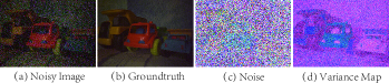
Figure 9: One typical visual example in SIDD [65] dataset. From left to right: (a) noisy image $\bm{y}$; (b) noise-free image $\bm{x}$; (c) image noise calculated through $|\bm{y}-\bm{x}|$; (d) variance map predicted by the proposed method.

Non-I.I.D. Gaussian Noise. In Sec. 5.1.1, we adopt three groups of noise variance maps (see Fig. 2 (b1-d1)) to synthesize the testing data, so as to evaluate the performance of VIRNet under the non-i.i.d. Gaussian noise. Correspondingly, Fig. 2 (b2-d2) further displays the variance maps predicted by VIRNet for easy visualization. It can be seen that these predicted variance maps have very similar spatial variation with the groundtruth ones, which are expected to facilitate the subsequent denoising task or other non-blind denoising methods. To justify this point, we also apply these predicted variance maps in FFDNet [20] to test its performance under the non-i.i.d. Gaussian noise, and the quantitative comparisons are listed in Table VIII. One can see that $\text{FFDNet}_{\text{VIR}}$ and $\text{FFDNet}_{\text{GT}}$ have very similar performance, and the performance difference between them is less than 0.04dB PSNR. This indicates that VIRNet is able to effectively handle such complicated noise distribution.

Signal-dependent Noise. The challenge in real-world image denoising is mainly attributed to the signal-dependentness of the image noise. Fig. 9 shows one typical real-world noisy example coming from SIDD [65] dataset and the corresponding variance maps predicted by VIRNet. Note that the variance map has been enlarged several times for easy visualization. It is easy to see that the estimated noise variance map depicts strong relevance to the pixel illumination, implying that the proposed VIRNet is able to finely approximate the signal-dependent real noise.

5.3.2 Kernel Estimation

As is well known, kernel estimation plays an important role in blind image super-resolution [103]. To evaluate the effectiveness of VIRNet in this subtask, we compare three recent kernel estimation methods specifically designed for super-resolution, including KernelGan [96], DIPFKP [63], and BSRDM [64]. Since these three methods are all relatively time-consuming, we randomly select 20 images from the validation set of DIV2K [92] (denoted as DIV2K20) as testing data. The LR images are synthesized using the last four anisotropic Gaussian kernels in Fig. 5 under a scale factor of 4, and the noise level is set as $2.55$.

As for the evaluation, we use two ways to compare the performance of different methods. Firstly, the mean square error (MSE) between the estimated kernel and the groudtruth kernel is an intuitive metric that directly reflects the accurancy of the estimate kernel. The detailed comparison results are listed in Table IX. Secondly, we apply the estimated blur kernels in a non-blind super-resolution method USRNet [56] and then compare the recovered HR image in terms of PSNR, SSIM [85], and LPIPS [95]. The comparison results on these three metrics are listed in Table X. From both tables, one can easily observe that the proposed VIRNet exhibits evident superiority over other competing methods.

5.4 Analysis on Posteriori Factorization

When designing the variational inference algorithm in Sec. 4, we factorize the variational distribution $q(\bm{z},\bm{\sigma}^{2},\bm{\varLambda}|\bm{y})$ into a conditional format of Eq. (12), which fundamentally induces the cascaded inference framework in Fig. 1. In fact, different factorized assumptions on $q(\bm{z},\bm{\sigma}^{2},\bm{\varLambda}|\bm{y})$ will lead to different designs on the inference framework. For example, the following unconditonal factorization

$$q(\bm{z},\bm{\sigma}^{2},\bm{\varLambda}|\bm{y})=q(\bm{z}|\bm{y})q(\bm{\sigma}^{2}|\bm{y})q(\bm{\varLambda}|\bm{y}),$$ (28)

will induce a parallel inference architecture. Specifically, the three sub-networks, namely SNet, KNet, and RNet, will feedforward independently in such a parallel framework, but they are able to interact during back propagation through ELBO. Please refer to our previous conference version [27] for a thorough overview on this point.

To validate the superiority of the conditional form of Eq. (12), we consider different posteriori factorizations and empirically compare their performance on the task of image super-resolution, since it involves more general degradations than image denoising. Table XI lists the average comparison results on DIV2K100 with a scale factor of 4. As compared with Baseline1, it can be seen that VIRNet achieves evident performance gain, which indicates that the degradation information (i.e., the noise level and the blue kernel) can facilitate the image restoration task. In fact, such a conditional factorization in VIRNet is consistent with the classical model-based methods that decompose the blind IR in two subproblems, namely degradation estimation and image restoration. The superiority of Baseline3 over Baseline2 demonstrates that the kernel information can bring up more marginal performance improvement than the noise level, complying with the conclusion in [103]. However, the performance gain of VIRNet over Baseline3 on LPIPS substantiates that conditioning on the noise level can further improve the perceptual quality of the recovered images.

6 Conclusion

In this paper, we have proposed a novel deep variational network for blind IR, which aims to finely integrate the merits of both classical model-based methods and recent DL-based methods. On one hand, we have constructed a Bayesian generative model for blind image denoising and image super-resolution, by carefully considering the image degradation from the perspectives of image noise and blur kernel. On the other hand, a variational inference algorithm has been elaborately designed to solve the proposed model, in which the posteriori distribution are all parameterized by DNNs to increase the non-linear fitting capability. Most notably, this variational algorithm induces a unified framework to simultaneously deal with the tasks of degradation estimation and image restoration. Extensive experiments have also been conducted to demonstrate the superiority of our method on image denoising and super-resolution. In the future, we will make further effort to extend our method to deal with more complicated and general image degradations.

References

- [1] Y. Tsin, V. Ramesh, and T. Kanade, “Statistical calibration of ccd imaging process,” in Proceedings of the IEEE/CVF International Conference on Computer Vision (ICCV), vol. 1, 2001, pp. 480–487.
- [2] L. I. Rudin, S. Osher, and E. Fatemi, “Nonlinear total variation based noise removal algorithms,” Physica D: nonlinear phenomena, vol. 60, no. 1-4, pp. 259–268, 1992.
- [3] A. Buades, B. Coll, and J.-M. Morel, “A non-local algorithm for image denoising,” in Proceedings of the IEEE/CVF Conference on Computer Vision and Pattern Recognition (CVPR), vol. 2, 2005, pp. 60–65.
- [4] K. Dabov, A. Foi, V. Katkovnik, and K. Egiazarian, “Image denoising by sparse 3-d transform-domain collaborative filtering,” IEEE Transactions on Image Processing, vol. 16, no. 8, pp. 2080–2095, 2007.
- [5] J. Mairal, M. Elad, and G. Sapiro, “Sparse representation for color image restoration,” IEEE Transactions on Image Processing, vol. 17, no. 1, pp. 53–69, 2007.
- [6] W. Dong, L. Zhang, G. Shi, and X. Li, “Nonlocally centralized sparse representation for image restoration,” IEEE Transactions on Image Processing, vol. 22, no. 4, pp. 1620–1630, 2012.
- [7] J. Xu, L. Zhang, and D. Zhang, “A trilateral weighted sparse coding scheme for real-world image denoising,” in Proceedings of the European Conference on Computer Vision (ECCV), 2018, pp. 20–36.
- [8] W. Dong, G. Shi, and X. Li, “Nonlocal image restoration with bilateral variance estimation: a low-rank approach,” IEEE Transactions on Image Processing, vol. 22, no. 2, pp. 700–711, 2012.
- [9] S. Gu, L. Zhang, W. Zuo, and X. Feng, “Weighted nuclear norm minimization with application to image denoising,” in Proceedings of the IEEE/CVF Conference on Computer Vision and Pattern Recognition (CVPR), 2014, pp. 2862–2869.
- [10] J. Xu, L. Zhang, D. Zhang, and X. Feng, “Multi-channel weighted nuclear norm minimization for real color image denoising,” in Proceedings of the IEEE/CVF International Conference on Computer Vision (ICCV), 2017, pp. 1096–1104.
- [11] D. Meng and F. De La Torre, “Robust matrix factorization with unknown noise,” in Proceedings of the IEEE/CVF International Conference on Computer Vision (ICCV), 2013, pp. 1337–1344.
- [12] X. Cao, Y. Chen, Q. Zhao, D. Meng, Y. Wang, D. Wang, and Z. Xu, “Low-rank matrix factorization under general mixture noise distributions,” in Proceedings of the IEEE/CVF International Conference on Computer Vision (ICCV), 2015, pp. 1493–1501.
- [13] F. Zhu, G. Chen, J. Hao, and P.-A. Heng, “Blind image denoising via dependent dirichlet process tree,” IEEE Transactions on Pattern Analysis and Machine Intelligence, vol. 39, no. 8, pp. 1518–1531, 2016.
- [14] Z. Yue, D. Meng, Y. Sun, and Q. Zhao, “Hyperspectral image restoration under complex multi-band noises,” Remote Sensing, vol. 10, no. 10, p. 1631, 2018.
- [15] Z. Yue, H. Yong, D. Meng, Q. Zhao, Y. Leung, and L. Zhang, “Robust multiview subspace learning with nonindependently and nonidentically distributed complex noise,” IEEE Transactions on Neural Networks and Learning Systems, 2019.
- [16] C. Dong, C. C. Loy, K. He, and X. Tang, “Learning a deep convolutional network for image super-resolution,” in Proceedings of the European Conference on Computer Vision (ECCV). Springer, 2014, pp. 184–199.
- [17] K. Zhang, W. Zuo, Y. Chen, D. Meng, and L. Zhang, “Beyond a gaussian denoiser: Residual learning of deep cnn for image denoising,” IEEE Transactions on Image Processing, vol. 26, no. 7, pp. 3142–3155, 2017.
- [18] X. Mao, C. Shen, and Y.-B. Yang, “Image restoration using very deep convolutional encoder-decoder networks with symmetric skip connections,” in Proceedings of the Advances in Neural Information Processing Systems (NeurIPS), 2016, pp. 2802–2810.
- [19] Y. Zhang, K. Li, K. Li, L. Wang, B. Zhong, and Y. Fu, “Image super-resolution using very deep residual channel attention networks,” in Proceedings of the European Conference on Computer Vision (ECCV), 2018, pp. 294–310.
- [20] K. Zhang, W. Zuo, and L. Zhang, “Ffdnet: Toward a fast and flexible solution for cnn-based image denoising,” IEEE Transactions on Image Processing, vol. 27, no. 9, pp. 4608–4622, 2018.
- [21] Y. Zhang, K. Li, K. Li, B. Zhong, and Y. Fu, “Residual non-local attention networks for image restoration,” in Proceedings of the International Conference on Learning Representations (ICLR), 2019.
- [22] S. Guo, Z. Yan, K. Zhang, W. Zuo, and L. Zhang, “Toward convolutional blind denoising of real photographs,” in Proceedings of the IEEE Conference on Computer Vision and Pattern Recognition (CVPR), 2019, pp. 1712–1722.
- [23] S. Anwar and N. Barnes, “Real image denoising with feature attention,” in Proceedings of the IEEE/CVF International Conference on Computer Vision (ICCV), October 2019, pp. 3155–3164.
- [24] Z. Yue, Q. Zhao, L. Zhang, and D. Meng, “Dual adversarial network: Toward real-world noise removal and noise generation,” in Proceedings of the European Conference on Computer Vision (ECCV). Springer, 2020, pp. 41–58.
- [25] S. W. Zamir, A. Arora, S. Khan, M. Hayat, F. S. Khan, M.-H. Yang, and L. Shao, “Multi-stage progressive image restoration,” in Proceedings of the IEEE/CVF Conference on Computer Vision and Pattern Recognition (CVPR), 2021, pp. 14 821–14 831.
- [26] J. Liang, G. Sun, K. Zhang, L. Van Gool, and R. Timofte, “Mutual affine network for spatially variant kernel estimation in blind image super-resolution,” in Proceedings of the IEEE/CVF International Conference on Computer Vision (ICCV), 2021, pp. 4096–4105.
- [27] Z. Yue, H. Yong, Q. Zhao, D. Meng, and L. Zhang, “Variational denoising network: Toward blind noise modeling and removal,” in Proceedings of Advances in Neural Information Processing Systems (NeurIPS), 2019, pp. 1688–1699.
- [28] E. P. Simoncelli and E. H. Adelson, “Noise removal via bayesian wavelet coring,” in Proceedings of the IEEE/CVF International Conference on Image Processing (ICCV), vol. 1, 1996, pp. 379–382.
- [29] S. Roth and M. J. Black, “Fields of experts,” International Journal of Computer Vision, vol. 82, no. 2, p. 205, 2009.
- [30] A. Barbu, “Learning real-time mrf inference for image denoising,” in Proceedings of the IEEE/CVF Conference on Computer Vision and Pattern Recognition (CVPR), 2009, pp. 1574–1581.
- [31] J. Sun and M. F. Tappen, “Separable markov random field model and its applications in low level vision,” IEEE Transactions on Image Processing, vol. 22, no. 1, pp. 402–407, 2012.
- [32] R. Vemulapalli, O. Tuzel, and M.-Y. Liu, “Deep gaussian conditional random field network: A model-based deep network for discriminative denoising,” in Proceedings of the IEEE/CVF Conference on Computer Vision and Pattern Recognition (CVPR), 2016, pp. 4801–4809.
- [33] P. Qiao, Y. Dou, W. Feng, R. Li, and Y. Chen, “Learning non-local image diffusion for image denoising,” in Proceedings of the ACM International Conference on Multimedia (MM), 2017, pp. 1847–1855.
- [34] F. Zhu, G. Chen, and P.-A. Heng, “From noise modeling to blind image denoising,” in Proceedings of the IEEE/CVF Conference on Computer Vision and Pattern Recognition (CVPR), 2016, pp. 420–429.
- [35] V. Jain and S. Seung, “Natural image denoising with convolutional networks,” in Proceedings of the Advances in Neural Information Processing Systems (NeurIPS), 2009, pp. 769–776.
- [36] J. Xie, L. Xu, and E. Chen, “Image denoising and inpainting with deep neural networks,” in Proceedings of the Advances in Neural Information Processing Systems (NeurIPS), 2012, pp. 341–349.
- [37] F. Agostinelli, M. R. Anderson, and H. Lee, “Adaptive multi-column deep neural networks with application to robust image denoising,” in Proceedings of the Advances in Neural Information Processing Systems (NeurIPS), 2013, pp. 1493–1501.
- [38] H. C. Burger, C. J. Schuler, and S. Harmeling, “Image denoising: Can plain neural networks compete with bm3d?” in Proceedings of the IEEE/CVF Conference on Computer Vision and Pattern Recognition (CVPR), 2012, pp. 2392–2399.
- [39] Y. Tai, J. Yang, X. Liu, and C. Xu, “Memnet: A persistent memory network for image restoration,” in Proceedings of the IEEE/CVF International Conference on Computer Vision (ICCV), 2017, pp. 4539–4547.
- [40] W. Shi, J. Caballero, F. Huszár, J. Totz, A. P. Aitken, R. Bishop, D. Rueckert, and Z. Wang, “Real-time single image and video super-resolution using an efficient sub-pixel convolutional neural network,” in Proceedings of the IEEE/CVF Conference on Computer Vision and Pattern Recognition (CVPR), 2016, pp. 1874–1883.
- [41] C. Ledig, L. Theis, F. Huszár, J. Caballero, A. Cunningham, A. Acosta, A. Aitken, A. Tejani, J. Totz, Z. Wang et al., “Photo-realistic single image super-resolution using a generative adversarial network,” in Proceedings of the IEEE/CVF Conference on Computer Vision and Pattern Recognition (CVPR), 2017, pp. 4681–4690.
- [42] X. Wang, K. Yu, S. Wu, J. Gu, Y. Liu, C. Dong, Y. Qiao, and C. C. Loy, “Esrgan: Enhanced super-resolution generative adversarial networks,” in Proceedings of the European Conference on Computer Vision Workshops (ECCVW), September 2018.
- [43] Y. Zhang, Y. Tian, Y. Kong, B. Zhong, and Y. Fu, “Residual dense network for image super-resolution,” in Proceedings of the IEEE/CVF Conference on Computer Vision and Pattern Recognition (CVPR), 2018, pp. 2472–2481.
- [44] J. Gu, H. Lu, W. Zuo, and C. Dong, “Blind super-resolution with iterative kernel correction,” in Proceedings of the IEEE/CVF conference on Computer Vision and Pattern Recognition (CVPR), 2019, pp. 1604–1613.
- [45] Y.-S. Xu, S.-Y. R. Tseng, Y. Tseng, H.-K. Kuo, and Y.-M. Tsai, “Unified dynamic convolutional network for super-resolution with variational degradations,” in Proceedings of the IEEE/CVF Conference on Computer Vision and Pattern Recognition (CVPR), 2020, pp. 12 496–12 505.
- [46] K. Zhang, J. Liang, L. Van Gool, and R. Timofte, “Designing a practical degradation model for deep blind image super-resolution,” in Proceedings of the IEEE/CVF International Conference on Computer Vision (ICCV), 2021, pp. 4791–4800.
- [47] I. Goodfellow, J. Pouget-Abadie, M. Mirza, B. Xu, D. Warde-Farley, S. Ozair, A. Courville, and Y. Bengio, “Generative adversarial nets,” in Proceedings of the Advances in Neural Information Processing Systems (NeurIPS), 2014, pp. 2672–2680.
- [48] J. Chen, J. Chen, H. Chao, and M. Yang, “Image blind denoising with generative adversarial network based noise modeling,” in Proceedings of the IEEE/CVF Conference on Computer Vision and Pattern Recognition (CVPR), 2018, pp. 3155–3164.
- [49] D.-W. Kim, J. Ryun Chung, and S.-W. Jung, “Grdn: Grouped residual dense network for real image denoising and gan-based real-world noise modeling,” in Proceedings of the IEEE/CVF Conference on Computer Vision and Pattern Recognition Workshops (CVPRW), 2019, pp. 0–0.
- [50] K. Zhang, W. Zuo, S. Gu, and L. Zhang, “Learning deep cnn denoiser prior for image restoration,” in Proceedings of the IEEE/CVF Conference on Computer Vision and Pattern Recognition (CVPR), 2017, pp. 3929–3938.
- [51] T. Tirer and R. Giryes, “Image restoration by iterative denoising and backward projections,” IEEE Transactions on Image Processing, vol. 28, no. 3, pp. 1220–1234, 2018.
- [52] E. Ryu, J. Liu, S. Wang, X. Chen, Z. Wang, and W. Yin, “Plug-and-play methods provably converge with properly trained denoisers,” in Proceedings of the International Conference on Machine Learning (ICML). PMLR, 2019, pp. 5546–5557.
- [53] K. Zhang, W. Zuo, and L. Zhang, “Deep plug-and-play super-resolution for arbitrary blur kernels,” in Proceedings of the IEEE/CVF Conference on Computer Vision and Pattern Recognition (CVPR), 2019, pp. 1671–1681.
- [54] K. Zhang, Y. Li, W. Zuo, L. Zhang, L. Van Gool, and R. Timofte, “Plug-and-play image restoration with deep denoiser prior,” IEEE Transactions on Pattern Analysis and Machine Intelligence, 2021.
- [55] T. Eboli, J. Sun, and J. Ponce, “End-to-end interpretable learning of non-blind image deblurring,” in Proceedings of the European Conference on Computer Vision (ECCV). Springer, 2020, pp. 314–331.
- [56] K. Zhang, L. V. Gool, and R. Timofte, “Deep unfolding network for image super-resolution,” in Proceedings of the IEEE/CVF Conference on Computer Vision and Pattern Recognition (CVPR), 2020, pp. 3217–3226.
- [57] L. Zhengxiong, Y. Huang, S. Li, L. Wang, T. Tan et al., “Unfolding the alternating optimization for blind super resolution,” Proceedings of the Advances in Neural Information Processing Systems (NeurIPS), vol. 33, pp. 5632–5643, 2020.
- [58] S. Kong, W. Wang, X. Feng, and X. Jia, “Deep red unfolding network for image restoration,” IEEE Transactions on Image Processing, vol. 31, pp. 852–867, 2021.
- [59] H. Zheng, H. Yong, and L. Zhang, “Deep convolutional dictionary learning for image denoising,” in Proceedings of the IEEE/CVF Conference on Computer Vision and Pattern Recognition (CVPR), 2021, pp. 630–641.
- [60] D. Ulyanov, A. Vedaldi, and V. Lempitsky, “Deep image prior,” in Proceedings of the IEEE/CVF Conference on Computer Vision and Pattern Recognition (CVPR), 2018, pp. 9446–9454.
- [61] Y. Gandelsman, A. Shocher, and M. Irani, “” double-dip”: Unsupervised image decomposition via coupled deep-image-priors,” in Proceedings of the IEEE/CVF Conference on Computer Vision and Pattern Recognition (CVPR), 2019, pp. 11 026–11 035.
- [62] D. Ren, K. Zhang, Q. Wang, Q. Hu, and W. Zuo, “Neural blind deconvolution using deep priors,” in Proceedings of the IEEE/CVF Conference on Computer Vision and Pattern Recognition (CVPR), 2020, pp. 3341–3350.
- [63] J. Liang, K. Zhang, S. Gu, L. Van Gool, and R. Timofte, “Flow-based kernel prior with application to blind super-resolution,” in Proceedings of the IEEE/CVF Conference on Computer Vision and Pattern Recognition (CVPR), 2021, pp. 10 601–10 610.
- [64] Z. Yue, Q. Zhao, J. Xie, L. Zhang, D. Meng, and K.-Y. K. Wong, “Blind image super-resolution with elaborate degradation modeling on noise and kernel,” in Proceedings of the IEEE/CVF Conference on Computer Vision and Pattern Recognition (CVPR), 2022.
- [65] A. Abdelhamed, S. Lin, and M. S. Brown, “A high-quality denoising dataset for smartphone cameras,” in Proceedings of the IEEE/CVF Conference on Computer Vision and Pattern Recognition (CVPR), 2018, pp. 1692–1700.
- [66] H. Yong, D. Meng, W. Zuo, and L. Zhang, “Robust online matrix factorization for dynamic background subtraction,” IEEE Transactions on Pattern Analysis and Machine Intelligence, vol. 40, no. 7, pp. 1726–1740, 2018.
- [67] G. Riegler, S. Schulter, M. Ruther, and H. Bischof, “Conditioned regression models for non-blind single image super-resolution,” in Proceedings of the IEEE/CVF International Conference on Computer Vision (ICCV), 2015, pp. 522–530.
- [68] K. Zhang, W. Zuo, and L. Zhang, “Learning a single convolutional super-resolution network for multiple degradations,” in Proceedings of the IEEE/CVF Conference on Computer Vision and Pattern Recognition (CVPR), 2018, pp. 3262–3271.
- [69] L. Wang, Y. Wang, X. Dong, Q. Xu, J. Yang, W. An, and Y. Guo, “Unsupervised degradation representation learning for blind super-resolution,” in Proceedings of the IEEE/CVF Conference on Computer Vision and Pattern Recognition (CVPR), 2021, pp. 10 581–10 590.
- [70] C. M. Bishop, Pattern Recognition and Machine Learning, 2006.
- [71] D. P. Kingma and M. Welling, “Auto-encoding variational bayes,” in Proceedings of the International Conference on Learning Representations (ICLR), 2014.
- [72] M. Jankowiak and F. Obermeyer, “Pathwise derivatives beyond the reparameterization trick,” in Proceedings of the International Conference on Machine Learning (ICML). PMLR, 2018, pp. 2235–2244.
- [73] Y. Quan, M. Chen, T. Pang, and H. Ji, “Self2self with dropout: Learning self-supervised denoising from single image,” in Proceedings of the IEEE/CVF Conference on Computer Vision and Pattern Recognition (CVPR), 2020, pp. 1890–1898.
- [74] T. Huang, S. Li, X. Jia, H. Lu, and J. Liu, “Neighbor2neighbor: Self-supervised denoising from single noisy images,” in Proceedings of the IEEE/CVF Conference on Computer Vision and Pattern Recognition (CVPR), 2021, pp. 14 781–14 790.
- [75] O. Ronneberger, P. Fischer, and T. Brox, “U-net: Convolutional networks for biomedical image segmentation,” in Proceedings of the International Conference on Medical Image Computing and Computer-assisted Intervention (MICCA). Springer, 2015, pp. 234–241.
- [76] K. He, X. Zhang, S. Ren, and J. Sun, “Deep residual learning for image recognition,” in Proceedings of the IEEE/CVF Conference on Computer Vision and Pattern Recognition (CVPR), 2016, pp. 770–778.
- [77] D. P. Kingma and J. L. Ba, “Adam: A method for stochastic optimization,” in ICLR 2015 : International Conference on Learning Representations 2015, 2015.
- [78] A. Paszke, S. Gross, F. Massa, A. Lerer, J. Bradbury, G. Chanan, T. Killeen, Z. Lin, N. Gimelshein, L. Antiga et al., “Pytorch: An imperative style, high-performance deep learning library,” Proceedings of the Advances in Neural Information Processing Systems (NeurIPS), vol. 32, 2019.
- [79] I. Loshchilov and F. Hutter, “Sgdr: Stochastic gradient descent with warm restarts,” in Proceedings of the International Conference on Learning Representations (ICLR), 2017.
- [80] P. Arbelaez, M. Maire, C. Fowlkes, and J. Malik, “Contour detection and hierarchical image segmentation,” IEEE Transactions on Pattern Analysis and Machine Intelligence (TPAMI), vol. 33, no. 5, pp. 898–916, 2010.
- [81] J. Deng, W. Dong, R. Socher, L.-J. Li, K. Li, and L. Fei-Fei, “Imagenet: A large-scale hierarchical image database,” in Proceedings of the IEEE/CVF Conference on Computer Vision and Pattern Recognition (CVPR), 2009, pp. 248–255.
- [82] K. Ma, Z. Duanmu, Q. Wu, Z. Wang, H. Yong, H. Li, and L. Zhang, “Waterloo exploration database: New challenges for image quality assessment models,” IEEE Transactions on Image Processing (TIP), vol. 26, no. 2, pp. 1004–1016, 2017.
- [83] L. Zhang, X. Wu, A. Buades, and X. Li, “Color demosaicking by local directional interpolation and nonlocal adaptive thresholding,” Journal of Electronic Imaging, vol. 20, no. 2, p. 23016, 2011.
- [84] T. Plotz and S. Roth, “Benchmarking denoising algorithms with real photographs,” in 2017 IEEE Conference on Computer Vision and Pattern Recognition (CVPR), 2017, pp. 2750–2759.
- [85] Z. Wang, A. Bovik, H. Sheikh, and E. Simoncelli, “Image quality assessment: from error visibility to structural similarity,” IEEE Transactions on Image Processing, vol. 13, no. 4, pp. 600–612, 2004.
- [86] Y. Kim, J. W. Soh, G. Y. Park, and N. I. Cho, “Transfer learning from synthetic to real-noise denoising with adaptive instance normalization,” in Proceedings of the IEEE/CVF Conference on Computer Vision and Pattern Recognition (CVPR), 2020, pp. 3482–3492.
- [87] M. Chang, Q. Li, H. Feng, and Z. Xu, “Spatial-adaptive network for single image denoising,” in Proceedins of the European Conference on Computer Vision (ECCV). Springer, 2020, pp. 171–187.
- [88] S. W. Zamir, A. Arora, S. Khan, M. Hayat, F. S. Khan, M.-H. Yang, and L. Shao, “Cycleisp: Real image restoration via improved data synthesis,” in Proceedings of the IEEE/CVF Conference on Computer Vision and Pattern Recognition (CVPR), 2020, pp. 2696–2705.
- [89] Y. Cai, X. Hu, H. Wang, Y. Zhang, H. Pfister, and D. Wei, “Learning to generate realistic noisy images via pixel-level noise-aware adversarial training,” Advances in Neural Information Processing Systems (NeurIPS), vol. 34, 2021.
- [90] B. Niu, W. Wen, W. Ren, X. Zhang, L. Yang, S. Wang, K. Zhang, X. Cao, and H. Shen, “Single image super-resolution via a holistic attention network,” in Proceeding of the European conference on computer vision (ECCV). Springer, 2020, pp. 191–207.
- [91] R. Zeyde, M. Elad, and M. Protter, “On single image scale-up using sparse-representations,” in Proceedings of the 7th international conference on Curves and Surfaces, 2010, pp. 711–730.
- [92] E. Agustsson and R. Timofte, “Ntire 2017 challenge on single image super-resolution: Dataset and study,” in Proceedings of the IEEE/CVF Conference on Computer Vision and Pattern Recognition Workshops (CVPRW), July 2017.
- [93] R. Timofte, E. Agustsson, L. Van Gool, M.-H. Yang, L. Zhang, B. Lim et al., “Ntire 2017 challenge on single image super-resolution: Methods and results,” in Proceedings of the IEEE/CVF Conference on Computer Vision and Pattern Recognition Workshops (CVPRW), July 2017.
- [94] A. Shocher, N. Cohen, and M. Irani, “Zero-shot super-resolution using deep internal learning,” in Proceedings of the IEEE/CVF Conference on Computer Vision and Pattern Recognition (CVPR), 2018, pp. 3118–3126.
- [95] R. Zhang, P. Isola, A. A. Efros, E. Shechtman, and O. Wang, “The unreasonable effectiveness of deep features as a perceptual metric,” in Proceedings of the IEEE/CVF conference on Computer Vision and Pattern Recognition (CVPR), 2018, pp. 586–595.
- [96] S. Bell-Kligler, A. Shocher, and M. Irani, “Blind super-resolution kernel estimation using an internal-gan,” Proceedings of Advances in Neural Information Processing Systems (NeurIPS), vol. 32, 2019.
- [97] A. Ignatov, N. Kobyshev, R. Timofte, K. Vanhoey, and L. Van Gool, “Dslr-quality photos on mobile devices with deep convolutional networks,” in Proceedings of the IEEE International Conference on Computer Vision (ICCV), 2017, pp. 3277–3285.
- [98] D. Martin, C. Fowlkes, D. Tal, and J. Malik, “A database of human segmented natural images and its application to evaluating segmentation algorithms and measuring ecological statistics,” in Proceedings of the IEEE/CVF International Conference on Computer Vision (ICCV), vol. 2, 2001, pp. 416–423.
- [99] Y. Matsui, K. Ito, Y. Aramaki, A. Fujimoto, T. Ogawa, T. Yamasaki, and K. Aizawa, “Sketch-based manga retrieval using manga109 dataset,” Multimedia Tools and Applications, vol. 76, no. 20, pp. 21 811–21 838, 2017.
- [100] C. Ma, C.-Y. Yang, X. Yang, and M.-H. Yang, “Learning a no-reference quality metric for single-image super-resolution,” Computer Vision and Image Understanding, vol. 158, pp. 1–16, 2017.
- [101] Y. Blau, R. Mechrez, R. Timofte, T. Michaeli, and L. Zelnik-Manor, “The 2018 pirm challenge on perceptual image super-resolution,” in Proceedings of the European Conference on Computer Vision Workshops (ECCVW), 2018, pp. 0–0.
- [102] X. Wang, L. Xie, C. Dong, and Y. Shan, “Real-esrgan: Training real-world blind super-resolution with pure synthetic data,” in Proceedings of the IEEE/CVF International Conference on Computer Vision (ICCV), 2021, pp. 1905–1914.
- [103] N. Efrat, D. Glasner, A. Apartsin, B. Nadler, and A. Levin, “Accurate blur models vs. image priors in single image super-resolution,” in Proceedings of the IEEE/CVF International Conference on Computer Vision (ICCV), 2013, pp. 2832–2839.