Joint Design of RF and gradient waveforms via auto-differentiation
for 3D tailored excitation in MRI

Abstract

This paper proposes a new method for joint design of radiofrequency (RF) and gradient waveforms in Magnetic Resonance Imaging (MRI), and applies it to the design of 3D spatially tailored saturation and inversion pulses. The joint design of both waveforms is characterized by the ODE Bloch equations, to which there is no known direct solution. Existing approaches therefore typically rely on simplified problem formulations based on, e.g., the small-tip approximation or constraining the gradient waveforms to particular shapes, and often apply only to specific objective functions for a narrow set of design goals (e.g., ignoring hardware constraints). This paper develops and exploits an auto-differentiable Bloch simulator to directly compute Jacobians of the (Bloch-simulated) excitation pattern with respect to RF and gradient waveforms. This approach is compatible with arbitrary sub-differentiable loss functions, and optimizes the RF and gradients directly without restricting the waveform shapes. For computational efficiency, we derive and implement explicit Bloch simulator Jacobians (approximately halving computation time and memory usage). To enforce hardware limits (peak RF, gradient, and slew rate), we use a change of variables that makes the 3D pulse design problem effectively unconstrained; we then optimize the resulting problem directly using the proposed auto-differentiation framework. We demonstrate our approach with two kinds of 3D excitation pulses that cannot be easily designed with conventional approaches: Outer-volume saturation ($90\mathrm{°}$ flip angle), and inner-volume inversion.

I Introduction

In a magnetic resonance imaging (MRI) experiment, the dynamic system relationship between the applied radiofrequency (RF) and gradient magnetic fields, and the instantaneous spin magnetization change they induce, is concisely described by the Bloch equation. While it is straightforward to calculate the magnetization pattern resulting from a given set of RF and gradient waveforms and tissue parameters, inverting the Bloch equation to obtain the waveforms that produce a given desired excitation pattern can be challenging.

This Bloch inversion task is conventionally called an “RF pulse design” problem, reflecting the fact that the most common way to design excitation pulses in MRI is to pre-define the gradients in some way, and then optimize only the (complex) RF waveform. Even with that simplification, the design problem remains non-linear and non-convex. Another common simplification is to apply the small-tip approximation [1] that can give reasonable excitation accuracy even for flip angles as high as $90\mathrm{°}$, at least for conventional 1D (slice-selective) excitations where the instantaneous flip angle during RF excitation remains relatively low. The small-tip approximation leads to a linear (Fourier) relationship between applied fields and the resulting magnetization pattern, and provides intuition about the excitation process by defining an “excitation k-space” trajectory and viewing RF transmission as depositing energy along that trajectory.

The more difficult problem of jointly optimizing both RF and gradient waveforms has been approached in various ways. Several methods are based on the small-tip approximation, and on optimizing the gradients over a restricted set of waveform shapes, such as “spoke” or “kt-point” locations in excitation k-space [2, 3, 4, 5, 6] or parameterized echo-planar or non-Cartesian trajectories [7, 8, 9, 10, 11]. A more general small-tip design approach for 3D tailored excitation used a B-spline parametrization of the gradient trajectory that is not restricted to particular fixed waveform shapes [12]. These approaches work well for small-tip excitations, but not for applications such as tailored saturation or inversion. In addition, even when the final desired flip angle is small, the instantaneous flip angle during RF excitation can be large enough to violate the small-tip assumption [13]. This model mismatch can cause noticeable differences between the Bloch-simulated excitation pattern and that predicted by the small-tip model used in the design.

Another limitation of previous approaches is that the design loss functions are typically limited to certain forms such as least squares (LS) based on the complex transverse excited magnetization, although adaptations to magnitude least squares (MLS) costs have been proposed [14]. Adding hardware constraints to the design formulation adds an additional layer of complexity that is often either ignored during pulse design, or controlled indirectly via, e.g., Tikhonov regularization of the RF waveform [6].

This work approaches the Bloch inversion task in a more direct and general way that is applicable to the joint design of RF and gradient waveforms for tailored multi-dimensional excitation in MRI. We temporally discretize the pulse, assuming piecewise constant gradient and RF within every time segment. Our method does not rely on the small-tip approximation, works for arbitrary sub-differentiable loss functions, and incorporates hardware constraints. Our approach contains three key elements: First, we derive analytic expressions for the Jacobian operations needed for the Bloch inversion for a unit (discrete) time step. Second, we incorporate these discrete-time Jacobian operations into an automatic differentiation framework [15], to obtain the Jacobian that relates the final magnetization pattern (at the end of the pulse) to the RF and gradient waveforms. Third, we enforce hardware limits by a change of variables that makes the optimization problem effectively unconstrained.

The paper is organized as follows. Section II gives a general form of the joint design problem, and derives the explicit Jacobians useful for accelerating the proposed auto-differentiation pulse design tools. Sections III and IV apply our pulse design tool to two large-tip excitation problems, and validate the results experimentally on a 3T MRI scanner. Sections V and VI discuss and conclude this work.

II Theory

II-A Problem Formation

We discretize 3D space on a regular grid with a total $n_{M}$ voxels ("spins"). These spins can have different parameters, e.g. T1, T2, and off-resonance. Let $n_{T}$ denote the length (number of time points) of the pulse to be designed. For (single coil) joint design of complex RF waveform $b\in\mathbb{C}^{n_{T}}$ and gradient $g\in\mathbb{R}^{n_{T}\times 3}$ we are interested in tackling the following general problem:

$$\begin{array}[]{cl}\underset{g\in\mathbb{R}^{n_{T}\times 3},\;b\in\mathbb{C}^{n_{T}}}{\operatorname*{arg\,min}}&\mathcal{L}\coloneqq f(M_{T}(g,b),M_{D})+\lambda\mathcal{R}\\ \text{s.~{}t.}&\|b\|_{\infty}\leq b_{\mathrm{max}}\\ &\|g\|_{\infty,\infty}\leq g_{\mathrm{max}}\\ &\|\mathsf{D}g\|_{\infty,\infty}\leq s_{\mathrm{max}},\\ \end{array}$$ (1)

where $\mathcal{L}$ is the loss function; $M_{D}\in\mathbb{R}^{n_{M}\times 3}$ is the target (Desired) magnetization pattern (a 3-dimensional magnetization vector at each spatial location); $M_{T}\in\mathbb{R}^{n_{M}\times 3}$ is the magnetization at the end of the pulse (time $T$) obtained by integrating the Bloch equation; $f$ is the excitation error metric (e.g., a common choice is least-square error of transverse magnetization, i.e., $\|M_{T}[\mathrel{\mathop{\mathchar 58\relax}},1{\mathrel{\mathop{\mathchar 58\relax}}}2]-M_{D}[\mathrel{\mathop{\mathchar 58\relax}},1{\mathrel{\mathop{\mathchar 58\relax}}}2]\|_{F}^{2}$); and $\mathcal{R}$ is an optional regularizer with weight $\lambda$ (a common choice is $\mathcal{R}=\|b\|_{2}^{2}$ to control peak RF amplitudes and SAR indirectly). For the constraints, we have $b_{\mathrm{max}}$, $g_{\mathrm{max}}$, and $s_{\mathrm{max}}$ for peak RF, gradient, and slew rate, respectively; $\mathsf{D}\in\mathbb{R}^{n_{T}\times n_{T}}$ is the temporal difference matrix divided by $\delta_{t}$, i.e., $\mathsf{D}g$ takes the 1st order temporal derivative of $g$ and yields the slew rate; and $\|\cdot\|_{\infty}$, and $\|\cdot\|_{\infty,\infty}$ are entry-wise norm returning the largest absolute value of the operand elements.

Problem (1) is challenging for two main reasons: First, the objective is non-convex with respect to its arguments, and is constrained. Second, neither $M_{T}(g,b)$, nor its Jacobians $\partial M_{T}/\partial g$ and $\partial M_{T}/\partial b$ that would be needed to directly minimize  (1), have an explicit expression in $g$ and $b$. To the best of our knowledge, existing methods all deal with simplifications of problem (1) based on, e.g., the small-tip, or spin domain models. In this work, we minimize (1) directly, and assume only that the temporal integration of the Bloch equation is well-approximated by a discrete-time Bloch simulator.

II-B Auto-Differentiation

We propose to compute the necessary derivatives using auto-differentiation [17], such that problem (1) can be optimized for arbitrary error metric $f$ and regularization $\mathcal{R}$. Auto-differentiation tools, e.g., PyTorch [15], decouples computations into stages, and constructs the Jacobian operations at each stage. These single-stage Jacobians are eventually combined using the chain rule. For instance, with a PyTorch based Bloch simulator that computes $M_{T}(g,b)$, one implicitly obtains $\partial M_{T}/\partial g$ and $\partial M_{T}/\partial b$. The loss derivatives with respect to the variables we wish to optimize, i.e., $\partial\mathcal{L}/\partial g$, and $\partial\mathcal{L}/\partial b$, can then be obtained by combining these expressions with $\partial\mathcal{L}/\partial M_{T}$. This approach allows us to directly optimize $g$ and $b$ with respect to arbitrary losses.

II-C Explicit Jacobian Operations

Auto-differentiation tools provide implicit Jacobian operations (also known as the default backward operations in auto-differentiation context) formed from tracking all elementary computations (e.g., addition, multiplication, etc). Such tools also allow users to substitute default Jacobian operations with their own implementations. In practice, such explicitly implemented Jacobian operations can be more efficient both computationally and memory-wise. Bloch simulation is typically the most computationally expensive stage in relating pulse waveforms to objective costs. Having explicit Jacobians of the Bloch simulator can therefore accelerate the computation.

To derive discrete time ($\delta_{t}$) explicit Jacobians in the rotating frame, for all magnetic spins, we assume equilibrium spin magnitudes of $1$, relaxation constants $e_{1}\coloneqq\exp(-\delta_{t}/T_{1})$, $e_{2}\coloneqq\exp(-\delta_{t}/T_{2})$, and gyromagnetic ratio $\gamma$. At time $t$, the rotating frame effective magnetic field (B-effective), $B_{t}\in\mathbb{R}^{3}$, causes the magnetic spin state $m_{t}\in\mathbb{R}^{3}$, to precess (rotate) about an axis $u_{t}\coloneqq B_{t}/\|B_{t}\|_{2}$ by angle $\phi_{t}\coloneqq-\gamma\delta_{t}\|B_{t}\|_{2}$. One iteration of discrete time Bloch simulation can be expressed as:

$$m_{t+1}=ER_{t}m_{t}+e,$$ (2)

where $E\coloneqq\operatorname{\mathsf{diag}}([e_{2},e_{2},e_{1}])$, $e\coloneqq[0,0,1-e_{1}]^{\mathsf{T}}$ model the relaxations; $R_{t}=\cos(\phi_{t})I+(1-\cos(\phi_{t}))u_{t}u_{t}^{\mathsf{T}}+\sin(\phi_{t})[u_{t}]_{\times}$ models the rotation; $I$ is the 3D identity matrix, $\operatorname{\mathsf{diag}}([1,1,1])$; and $[u_{t}]_{\times}$ denotes the cross product matrix of $u_{t}$, i.e., $[u_{t}]_{\times}m_{t}=u_{t}\times m_{t}$. The rotation matrix $R_{t}$ is spatially dependent, as it accounts for B-effective which incorporates applied gradients, off-resonance, etc. Relaxation terms, as they depend on the underlying tissue property, are generally also spatially dependent. To avoid notation clutter, we have not indicated those spatial dependencies in Eq. (2); rather, Eq. (2) can be considered to hold for a single spin isochromat, with the appropriate $R_{t}$ and relaxation terms for that isochromat.

One can verify the following recursive expressions for partial derivatives of the loss with respect to $m_{t}$ and $B_{t}$:

$$\dfrac{\partial{}\mathcal{L}}{\partial{m_{t}}} =R_{t}^{\mathsf{T}}E\dfrac{\partial{}\mathcal{L}}{\partial{m_{t+1}}}\eqqcolon h_{t},$$ (3)

$$\dfrac{\partial{}\mathcal{L}}{\partial{B_{t}}} =\gamma\delta_{t}/\phi_{t}(u_{t}u_{t}^{\mathsf{T}}-I)\dfrac{\partial{}\mathcal{L}}{\partial{u_{t}}}-\gamma\delta_{t}\dfrac{\partial{}\mathcal{L}}{\partial{\phi_{t}}}u_{t},$$

$$\dfrac{\partial{}\mathcal{L}}{\partial{u_{t}}} =\phi_{t}\left(\mathfrak{c}_{t}(m_{t}u_{t}^{\mathsf{T}}+m_{t}^{\mathsf{T}}u_{t}I)+\mathfrak{s}_{t}[m_{t}]_{\times}\right)Eh_{t+1},$$

$$\dfrac{\partial{}\mathcal{L}}{\partial{\phi_{t}}} =([u_{t}]_{\times}R_{t}m_{t})^{\mathsf{T}}Eh_{t+1},$$

where $\mathfrak{c}_{t}\coloneqq\left(1-\cos(\phi_{t})\right)\!/\phi_{t}$, $\mathfrak{s}_{t}\coloneqq\sin(\phi_{t})/\phi_{t}$. Given $\partial B_{t}/\partial g_{t}$ and $\partial B_{t}/\partial b_{t}$ (which are easy to compute), we obtain the necessary derivatives for the joint optimization by the chain rule:

$$\dfrac{\partial{}\mathcal{L}}{\partial{g_{t}}}=\dfrac{\partial{}\mathcal{L}}{\partial{B_{t}}}\cdot\dfrac{\partial{}B_{t}}{\partial{g_{t}}},\quad\dfrac{\partial{}\mathcal{L}}{\partial{b_{t}}}=\dfrac{\partial{}\mathcal{L}}{\partial{B_{t}}}\cdot\dfrac{\partial{}B_{t}}{\partial{b_{t}}}.$$

Using the explicit Jacobians in (3) for the Bloch simulator operations halved both the computation time and memory use compared to the default implicit Jacobian operations provided by PyTorch (v1.3).

The remaining Jacobians, such as $\partial\mathcal{L}/\partial M_{T}$, $\partial B_{t}/\partial b_{t}$, and $\partial B_{t}/\partial g_{t}$, typically do not involve complicated computations. Also, they can vary with different objectives, e.g., switching from LS to MLS; or with different excitation settings, e.g., uniform vs non-uniform transmit sensitivities. For program generality, we left these remaining Jacobians to be obtained implicitly by the auto-differentiation framework.

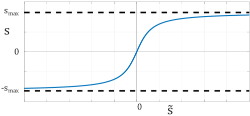
Figure 1: Turning constrained slew rate $s$ into unconstrained $\tilde{s}$, by change of variable tan^-1.

II-D Constraints

Constrained optimization often requires extra effort to ensure solution feasibility, such as feasible set projection and constraint substitution with penalizations. This would involve crafting projection algorithms, and tuning penalty parameters. For problem (1), in the absence of convexity, we use a change of variables [18, 19] that converts the problem into an effectively unconstrained one and avoids such extra effort during optimization.

Let $s\in\mathbb{R}^{n_{T}\times 3}$ denote the slew rate, i.e., $s=\mathsf{D}g$. Define $\tilde{s}=\tan(\pi/2\cdot s/s_{\mathrm{max}})$; $\tilde{\rho}\coloneqq\tan(\pi/2\cdot|b|/b_{\mathrm{max}})$, $\theta\coloneqq\angle b$. We automatically have $\|b\|_{\infty}\leq b_{\mathrm{max}}$ and $\|s\|_{\infty,\infty}\leq s_{\mathrm{max}}$ always satisfied (Fig. 1). Thus, we reformulate problem (1) as:

$$\begin{array}[]{cl}\underset{\tilde{s}\in\mathbb{R}^{n_{T}\times 3};\;\tilde{\rho},\;\theta\in\mathbb{R}^{n_{T}}}{\operatorname*{arg\,min}}&\mathcal{L}\coloneqq f(M_{T}(g,b),M_{D})+\lambda\mathcal{R}\\ \textrm{s. t.}&\|g\|_{\infty,\infty}\leq g_{\mathrm{max}}\\ &\mathsf{D}g=2s_{\mathrm{max}}/\pi\cdot\tan^{-1}(\tilde{s})\\ &b=2b_{\mathrm{max}}/\pi\cdot\exp(\iota\theta)\tan^{-1}(\tilde{\rho}).\\ \end{array}$$ (4)

In practice, for change of variable, $\tan^{-1}$ can be replaced with any other strictly monotone function, e.g., sigmoid, that maps an unconstrained domain to an interval.

Empirically, for 3D tailored pulse design, we observe that, with extended kt-points initializations [12], gradient amplitudes are well below typical max gradient constraints ($5\text{\,}\mathrm{G}\text{\,}{\mathrm{cm}}^{-1}$) prior to and throughout the optimization procedure. Hence, while problem (4) is still constrained formally, its max gradient is practically inactive. We thus treated it as an unconstrained problem for the results shown in this paper.

II-E Optimization Algorithm

We select initial waveforms $g$ and $b$ that satisfy the constraints. To minimize (4), we alternatingly update $\tilde{\rho}$, $\theta$, and $\tilde{s}$, as shown in Algorithm 1. This alternating strategy is commonly used in existing joint design approaches [12, 7], and helps reduce the problem size for the L-BFGS algorithm used in updating the pulse. With auto-differentiation, the optimization algorithm can be formulated without reference to the specific loss function, as demonstrated with very different design problems in section III. We use the L-BFGS optimizer provided by PyTorch for updating the variables within an iteration. The number of iterations may depend on pulse initializations. We empirically choose $N=10$ for experiments in this work. This choice can vary with applications.

Algorithm 1 Alternating Minimization

1:Inputs: Variables: $g$, $b$; Number of iterations: $N$

2:Compute $\tilde{\rho}$, $\theta$ and $\tilde{s}$ from $g$, $b$

3:for $n$ = 1 to $N$ do

4:     Fix $\tilde{s}$; Optimize $\tilde{\rho}$, $\theta$, using L-BFGS

5:     Fix $\tilde{\rho}$, $\theta$; Optimize $\tilde{s}$, using L-BFGS

6:end for

7:Compute $g$ and $b$, from $\tilde{\rho}$, $\theta$ and $\tilde{s}$

8:return $g$, $b$

III Methods

To demonstrate the utility and generality of our approach, we designed two different kinds of 3D tailored pulses: outer-volume (OV) saturation, and inner-volume (IV) inversion.

III-A 3D Outer-Volume Saturation Pulse Design

Outer-volume saturation pulses can be used to limit the imaging field of view (FOV), and hence has the potential to reduce both the time needed for data acquisition as well as motion artifacts from, e.g., the chest wall or abdomen in body imaging applications [20, 21, 22]. OV saturation pulses should ideally have a high flip angle in the OV region (e.g., 90 degrees), while leaving the IV unperturbed. These pulses are typically followed immediately by a gradient crusher. Since the phase of OV magnetization prior to the crusher is unimportant, we use MLS loss in design, and include a regularization term on RF power to indirectly control SAR as well as to demonstrate the generality of our approach:

$$\mathcal{L}_{90}=\||M_{T}[\mathrel{\mathop{\mathchar 58\relax}},1{\mathrel{\mathop{\mathchar 58\relax}}}2]|-|M_{D}[\mathrel{\mathop{\mathchar 58\relax}},1{\mathrel{\mathop{\mathchar 58\relax}}}2]|\|_{2}^{2}+\lambda\|b\|_{2}^{2},$$ (5)

where, $|M[\mathrel{\mathop{\mathchar 58\relax}},1{\mathrel{\mathop{\mathchar 58\relax}}}2]|\coloneqq\mathrm{abs}(M[\mathrel{\mathop{\mathchar 58\relax}},1]+\iota M[\mathrel{\mathop{\mathchar 58\relax}},2])$, is a vector function computing magnitudes of spin transverse magnetizations. For the target excitation profile, we set rows in $M_{D}$ to $[1,0,0]$ for OV spins, and $[0,0,1]$ for IV spins. We implemented this loss in PyTorch to obtain the Jacobian $\partial\mathcal{L}_{90}/\partial M_{T}$ as described in the Theory section.

In principle, small-tip based 3D tailored design approaches can also be applied to this loss by scaling the designed RF pulse to attain the desired $90\mathrm{°}$ flip (although the resulting pulse may exceed peak RF limits). We therefore compare our approach with the small-tip method in [12], starting with the same initial $b$ and $g$ waveforms in both cases (initialized as described in III-C).

III-B Inner-Volume Inversion Pulse Design

Next we designed another type of excitation pulse that is difficult to design using conventional approaches: an IV inversion pulse. Such a pulse may be useful for, e.g., selective inversion of arterial blood for flow territory mapping in perfusion imaging. For this pulse we propose a very different excitation loss based on the longitudinal magnetization:

$$\mathcal{L}_{180}=\|M_{T}[\mathrel{\mathop{\mathchar 58\relax}},3]-M_{D}[\mathrel{\mathop{\mathchar 58\relax}},3]\|_{2}^{2}+\lambda\|b\|_{2}^{2}.$$ (6)

We set rows in $M_{D}$ to $[0,0,1]$ for OV spins, and $[0,0,-1]$ for IV spins. We also implement this loss in PyTorch.

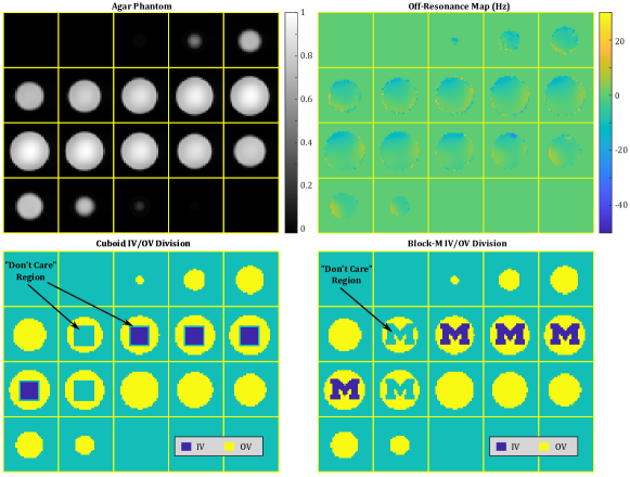
Figure 2: Experimental phantom, and the two target patterns (IV/OV divisions) used in our experiments. Top left: Magnitude image of the uniform Agar phantom. Top right: Observed field map, used in the pulse design to account for B0 inhomogeneity. A conservative mask that is 1-voxel-wide larger than the phantom support was used to ensure that the phantom boundary was included in the design. This expanded mask is the likely cause for the relatively large B0 values in some pixels at the edge of the mask (that are likely just outside the phantom). Bottom: Cuboid (left) and “block-M” (right) target patterns. We prescribed a “don’t care” (region with arrows) at the boundary between the IV and OV regions that is excluded when calculating the design loss. For the cuboid pattern, the don’t care region included the entire 3D IV/OV boundary, whereas for the block-M pattern, only the top and bottom slices (slices 6 and 11; slice numbers increase left-to-right and top-to-bottom) were included due to the low in-plane spatial resolution of the design grid.

III-C Pulse Initializations

The loss in problem (4) is non-convex, and the choice of initial $g$ and $b$ waveforms influences the final excitation result. How best to initialize these waveforms is an open problem. In [12], the initialization problem (in the context of small-tip 3D tailored excitation) was addressed by evaluating two popular choices for the excitation k-space trajectory, stack-of-spirals and SPINS [11], along with a novel alternative approach, “extended kt-points”, that chooses gradients based on the desired (target) excitation pattern. Sun et al. showed that the extended kt-points approach produces comparable or better excitation accuracy than stack-of-spirals or SPINS [12], so we chose it for the experiments in this work.

Once the gradients were initialized in this way, we initialized $b$ using the approach in [23]. These initial RF waveforms were scaled down when necessary to satisfy the $b_{\mathrm{max}}$ constraint.

III-D B-effective Computation

The particular form of B-effective depends on the excitation objective and other application-specific components. Besides the RF and gradient waveforms, it often also contains an off-resonance map (that may vary with time) and transmit sensitivity maps. Other factors such as gradient non-linearity can also be included in B-effective. For the single transmit coil phantom studies in this work, B-effective accounts for RF, gradient, and a static off-resonance map. Specifically, at time $t$, let $b_{t}\in\mathbb{C}$ and $g_{t}\in\mathbb{R}^{3}$ denote the instantaneous RF and gradients, respectively. For position $r$ relative to the scanner iso-center, with off-resonance $\omega(r)$, the instantaneous B-effective is:

$$B_{t}=[\mathfrak{R}(b_{t}),\mathfrak{I}(b_{t}),\langle g_{t},r\rangle+\omega(r)/\gamma],$$ (7)

where $\mathfrak{R}$ and $\mathfrak{I}$ extract the real and imaginary component, respectively.

TABLE I: Pulse Duration and TR/TE

Parameters	OV90	IV180	IV180M
Pulse Duration	$6.5\text{\,}\mathrm{ms}$	$4.8\text{\,}\mathrm{ms}$	$4.5\text{\,}\mathrm{ms}$
TR / TE	$2\text{\,}\mathrm{s}$ / $15\text{\,}\mathrm{ms}$	$3\text{\,}\mathrm{s}$ / minimum TE

III-E Phantom Experiments

We performed validation experiments in an Agar phantom on a GE MR750 3T scanner. Fig. 2 illustrates the experimental setup, including the prescribed IV and OV regions. All experiments used the same observed off-resonance map in the pulse design (Fig. 2). We used $T_{1}=$1.47\text{\,}\mathrm{s}$$, $T_{2}=$70\text{\,}\mathrm{ms}$$ in the Bloch simulation during designs. For all studies, we conducted the 3D design on a $32\text{\times}32\text{\times}20$ voxel grid of FOV $24\text{\times}24\text{\times}24\text{\,}\mathrm{cm}$; with RF power weighting coefficient $\lambda=4$, and constraints: $b_{\mathrm{max}}=$0.25\text{\,}\mathrm{G}$$, $g_{\mathrm{max}}=$5\text{\,}\mathrm{G}\text{\,}{\mathrm{cm}}^{-1}$$, $s_{\mathrm{max}}=$12\text{\,}\mathrm{G}\text{\,}{\mathrm{cm}}^{-1}\text{\,}{\mathrm{ms}}^{-1}$$. We quantified excitation performance in simulations with normalized root mean squared error (NRMSE). Spins in “don’t care” regions (Fig. 2) were excluded when calculating the NRMSE. We ran our design programs on an NVidia 2080 Ti graphics card. With the settings above, our method uses around $1.1\text{\,}\mathrm{GB}$ GPU RAM for all 3 designs. This includes the intrinsic GPU RAM usage of the PyTorch environment.

We performed three different experiments: 1. OV $90\mathrm{°}$ excitation using the cuboid target pattern shown in Fig. 2 (OV90); 2. IV inversion using that same cuboid target pattern (IV180); and 3. IV inversion with a block-M target pattern (IV180M). The experiments were implemented using a vendor-agnostic platform for rapid prototyping of MR pulse sequences [24, 25]. IV dimensions were $9\text{\times}9\text{\times}4.8\text{\,}\mathrm{cm}$ and $9\text{\times}12.8\text{\times}4.8\text{\,}\mathrm{cm}$ for the cuboid and block-M target patterns, respectively. We used a single channel transmit/receive birdcage coil for all experiments and assumed uniform RF transmit sensitivity during pulse design. To mitigate Gibbs ringing artifacts, we acquired the phantom images at a matrix size of $120\text{\times}120\text{\times}48$ and then downsized in image space to match the design grid size $32\text{\times}32\text{\times}20$.

We used long TR to wait for spin full recovery from saturation and inversion. For the OV90 experiment, as a substantial volume of the phantom is excited with large angle, we used TE=$15\text{\,}\mathrm{ms}$ to intentionally decay signal intensity and avoid saturating amplifiers in signal receiver during acquisition. We use minimum TE for the inversion experiments.

Figure 3: Schematic diagram of the imaging sequence used to characterize (validate) the 3D tailored inversion pulses.

For inversion performance validation, we use the sequence in Fig. 3 to obtain both phase and magnitude phantom images, with tip-down angle set to $10\mathrm{°}$. We expect a $\pi$ phase difference between inverted (IV) non-inverted (OV) regions, as the excitation pulse should tip inverted and non-inverted spins in opposite directions. In addition to the IV180 and IV180M excitation pulses, we imaged the phantom using the same sequence settings (TE/TR, flip angle, matrix size) using a conventional slab-selective Shinnar-Le Roux (SLR) pulse. We normalized the inversion images using this “non-inversion” image to eliminate receive coil sensitivity weighting (both magnitude and phase) in the inversion images. For completeness, the unnormalized images are shown in supplemental materials (Fig. S5).

IV Results

IV-A OV90

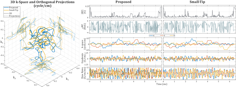
Figure 4: OV saturation pulses for the cuboid IV (Fig. 2), designed with our approach (Proposed) and the small-tip method in [12] (experiment OV90). The left panel shows the 3D k-space trajectories and their orthogonal projections: The two trajectories explore largely overlapping regions in excitation k-space. The right two panels show RF, gradient, and slew rate waveforms. Both designs satisfy the constraints, but for the small-tip design it was necessary to apply the VERSE [26] algorithm near the end of the pulse (see Discussion). Gradient peak amplitudes remain quite small ($\ll$5\text{\,}\mathrm{G}\text{\,}{\mathrm{cm}}^{-1}$$), whereas the gradient slew rates are frequently near their limit.

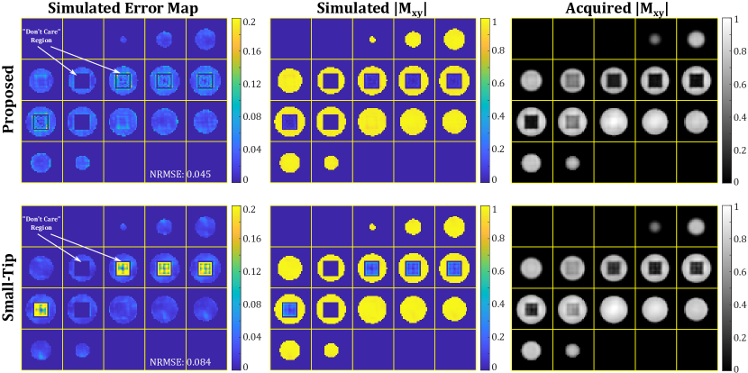
Figure 5: Experimental validation of the pulses shown in Fig. 4. The left panel shows the error map from simulation. Our approach has much smaller (-46%) NRMSE in simulation compared to Small-Tip. Acquired results (right) agree with the simulations (middle). Small-Tip approach has larger error inside the IV: This is expected, as the method produces only small-tip pulses, that we then scaled to meet the large-tip objective. The scaling increases excitation error inside IV while reducing error in the OV. Our approach directly designs large-tip pulses without this type of ‘scaling’ error.

Figure 4 shows the OV saturation pulses obtained with the proposed method and the small-tip approach in [12], and Fig. 5 shows the corresponding phantom imaging results. To keep the small-tip RF pulse within peak amplitude limits, we applied VERSE [26] near the end of the pulse. Our approach required $10\text{\,}\min$ for design, longer than the small-tip approach ($2\text{\,}\min$). While the RF waveforms differ markedly, the (excitation) k-space trajectories are more similar, though differences are clearly observed in the 3D trajectory plot (Fig. 4).

We observe excellent agreement between simulated and acquired excitation patterns (Fig. 5). Also, the proposed method produces much lower excitation error than the small-tip design (46% lower NRMSE error overall); this is expected as the small-tip assumption is violated after scaling the RF to attain the desired $90\mathrm{°}$ flip angle in the OV, which reduces the error in the OV at the expense of increased error in the IV.

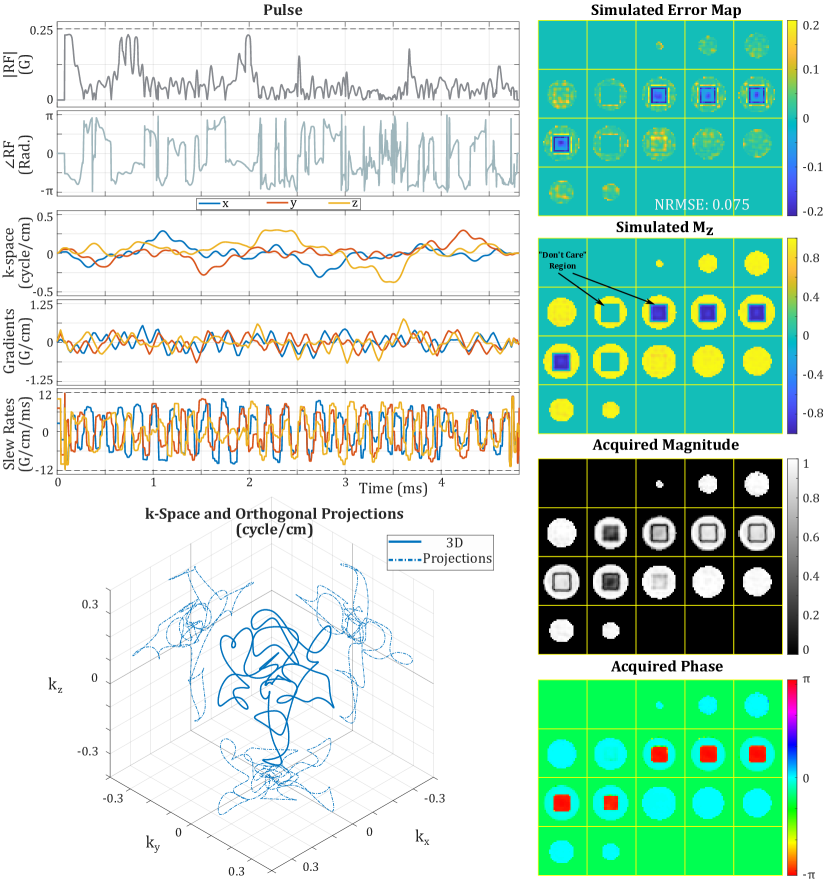
Figure 6: IV inversion results for the cuboid IV pattern (Experiment IV180). As desired, the $4.2\text{\,}\mathrm{ms}$ pulse satisfies all constraints. The gradient waveform is again far from its peak constraint of $5\text{\,}\mathrm{G}\text{\,}{\mathrm{cm}}^{-1}$. Compared to the OV90 experiment, the pulse has more extreme slew rate waveforms. The acquired magnitude and phase (i.e., the “observed inversion”) were obtained with the sequence in Fig. 3. We observe good agreement between simulated and acquired inversion patterns. The designed pulse successfully inverts the IV, as indicated by similar magnitude image intensity in the IV and OV regions (apart from transmit/receive coil shading) and a $\pi$ phase shift across the IV/OV boundary. The dark bands in the acquired images at the IV/OV boundary are due to spin saturation from incomplete inversion (and overlap substantially with the prescribed “don’t care” region).

IV-B IV180

Fig. 6 shows the results of the cuboid IV inversion experiment. Pulse waveforms and images from simulation and phantom experiments are shown. Pulse design took $6\text{\,}\min$. Simulations and acquired images are in excellent agreement, and indicate successful inversion within the IV with errors mainly located at the IV/OV boundary as expected. In particular, we observe dark bands along the IV/OV boundary in the magnitude image. Spins in this region are not fully inverted, resulting in low signal intensities in the magnitude image. The phase image shows an abrupt $\pi$ transition at the IV/OV boundary, indicating successful IV inversion.

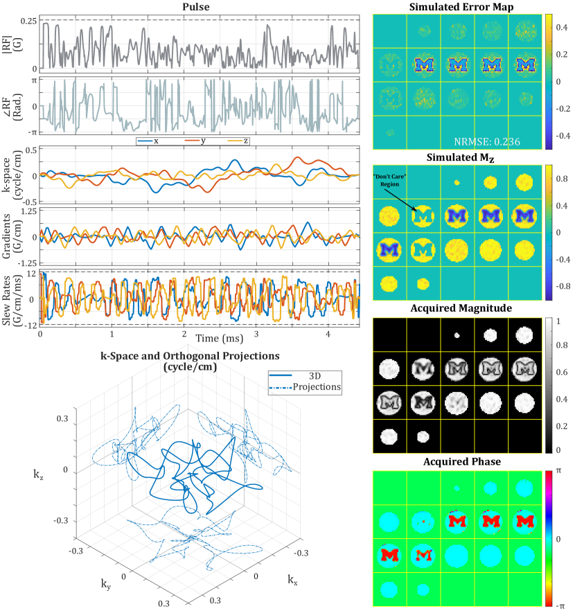
Figure 7: IV inversion results for the block-M target pattern (Experiment IV180M). The $4.5\text{\,}\mathrm{ms}$ pulse satisfies all constraints. The gradient waveforms are again well below the peak amplitude constraint of $5\text{\,}\mathrm{G}\text{\,}{\mathrm{cm}}^{-1}$, and slew rates are near the constraint for significant portions of the waveform duration. As in Fig. 6, the pulse successfully inverts the IV. The dark bands in the acquired magnitude image at the IV/OV boundary are due to saturation effects arising from the finite resolution (excitation k-space extent) of the pulse – even though only slices 6 and 11 were included in the “don’t care” region in the design due to the low in-plane spatial resolution of the design grid (see Fig. 2).

IV-C IV180M

Fig. 7 shows the results of the block-M IV inversion experiment. Pulse design took $6\text{\,}\min$. Slew rates are near the limit, similar to the IV180 experiment. Simulation and acquired images again indicate successful inversion. The NRMSE is larger than in the IV180 experiment, suggesting a trade-off between geometry complexity and excitation accuracy. Excitation error is largest near the in-plane edge of the block-M, where target $M_{z}$ changes sharply from $1$ to $-1$. We again observe dark bands along the IV/OV boundary, and an abrupt phase change across that boundary, as expected.

V Discussion

We have demonstrated a new approach to joint multi-dimensional excitation pulse design that directly optimizes both RF and gradient waveforms. Our approach is not limited to small-tip design problems, and is compatible with quite general loss/design functions such as those that involve longitudinal and/or magnitude magnetization. We validated our approach with 3D tailored large-tip objectives. For this type of application, the “extended kt-points” small-tip initialization [12] led to excellent large-tip results.

We chose to implement our auto-differentiable Bloch simulator with B-effective as its input for its generality: one can possibly prepend to it arbitrary functions that compute B-effective from various parameters, such as multi-coil parallel transmit (pTx) sensitivities, spin movements, and even non-linear response of gradient amplifiers, gradient delays, etc. This choice that favors generality may require more memory than software designs that take RF and gradients as inputs directly, and may require more expensive hardware with adequate memory for high-dimensional design problems. In particular, an interface that uses RF, gradient and spin location inputs requires a memory size proportional to $(N_{T}+N_{T}\times 3+N_{M}\times 3)$, whereas our interface requires memory proportional to $(N_{M}\times 3\times N_{T}+N_{M}\times 3)$. Our implementation can find use in different scenarios for proof-of-principle designs that one could then follow by customized simulators that meet specific computational requirements.

For the Bloch simulator, one may alternatively consider using the hard pulse approximation, which splits the instantaneous rotation matrix $R_{t}$ into two rotations: RF rotation, and transversal rotation due to the applied gradients and off-resonance. The hard pulse approximation is the basis for the SLR pulse design algorithm, and is crucial for the development of that algorithm. In our case, however, such splitting actually increases the number of elementary computations: when multiplying a vector, RF and transversal rotations require 9 and 4 multiplications, respectively, while direct multiplication by $R_{t}$ requires only 9. We therefore believe that the hard pulse approximation does not confer any particular advantages on our approach.

Apart from the explicit Jacobians introduced here, additional steps may be taken to reduce computation time. Computation time is primarily determined by pulse length, and not on the grid size (number of voxels) since computations are done voxel-wise and can be easily parallelized to within GPU RAM limits. Apart from increasing the simulation expense, longer pulses may also slow down Algorithm 1, since we used L-BFGS for updating RF and gradients. In the future, to shorten the optimization time for online pulse design tasks, it may be helpful to use coarser $\delta_{t}$ in the Bloch simulation [27] (here we used $4\text{\,}\mathrm{\SIUnitSymbolMicro s}$ to match our scanner’s hardware dwell time), or parameterize the gradient waveforms to reduce the optimization problem size (e.g., using B-splines as in [12]).

For the experiments presented, we used voxel resolution $7.5\text{\times}7.5\text{\times}12\text{\,}\mathrm{mm}$ and grid size $32\text{\times}32\text{\times}20$ for the pulse design. For more complex target excitation patterns and/or a larger FOV (e.g., as in the ISMRM parallel transmit pulse design challenge [28]), it may be desirable to increase the spatial resolution (maximum extent in excitation k-space) and/or grid size for finer excitation accuracy control. For instance, with a larger grid size, we would have space for in-plane “don’t care” region for the IV180M experiment, which may help reduce excitation error. A larger grid size will increase the memory usage in simulation, for which the use of multiple graphics cards may be needed to parallelize simulations across voxels.

In the OV90 experiment (Figs. 4–5), we were able to apply VERSE [26, 29] to the pulse designed with the small-tip approach [12] to avoid violating the RF amplitude limit (after scaling to attain $90\mathrm{°}$ flip angle in the OV). However, this adjustment was possible only because the $6.5\text{\,}\mathrm{ms}$ pulse happened to exceed peak RF only near the end of the pulse, allowing us to apply the VERSE strategy in a relatively straightforward way. In the more general case, where peak RF is exceeded during the middle of the pulse, it is more difficult to apply the VERSE technique to 3D RF pulses such as those designed here. We found empirically that in the OV90 experiment, shorter pulses designed with the small-tip approach tended to exceed peak RF during one or more intermediate intervals (after scaling), and that we were therefore unable to carry out an effective experimental evaluation for the purposes of the comparison presented here (Figs. 4–5). The proposed approach avoids this difficulty because peak RF is constrained as described in II-D; our approach was in fact able to design a shorter ($4\text{\,}\mathrm{ms}$) OV saturation pulse with the same excitation error as in Fig. 5 (not shown). In future work, a design approach that integrates VERSE into our method may be useful to further shorten a pulse for a given excitation objective.

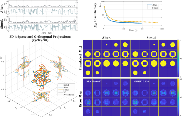
Figure S6: Comparison of alternating (Alter.) and Simultaneous (Simul.) minimization. The two approaches find similar but different local minima according to the RF and k-space plots (Left Panel). On the Top Right, the loss for the first 40 iterations is plotted. The computation time for each iteration is slightly longer for the simultaneous L-BFGS updates. The simultaneous updating scheme converges slightly slower, while the eventual excitation performance of the two schemes is comparable (Lower Right).

Pulse design problems are in general non-convex in terms of $b$ and $g$. Due to a lack of theoretical tools for non-convex problem convergence analysis, it is unclear how to best design an optimization algorithm for such problems a priori. In Algorithm 1, instead of simultaneously updating both RF and gradient waveforms, we chose to update them alternatingly as often done in existing small-tip joint designs [12, 30, 2, 7]. In supplemental Figs. S6-S7, we compared the alternating scheme with the simultaneous scheme, and found empirically that the alternating scheme optimizes faster than the simultaneous scheme for the specific problem settings we have in this work. Unfortunately, the non-convexity prevents us from fully comprehending this behavior, and we make no claims that the alternating approach used here is optimal over the many possible alternatives. Iteration stopping criteria for updating $b$ and $g$ are also commonly chosen ad hoc. Besides limiting the maximum number of iterations as we have done in Algorithm 1, another option can be setting a threshold to assert large-enough loss decreases and/or updates of the variables at each iteration. However, due to the $\tan^{-1}$ change of variables, a minuscule update of $b$ and $s$ near their limits will be mapped to a vast difference in the optimization variables $\tilde{\rho}$ and $\tilde{s}$, respectively. As an alternative to the updates of variables, one can threshold the norms of variable derivatives, or the change of $b$ and $s$ as the iteration stopping criteria.

Our approach may remind readers of optimal control (OC) based pulse design methods [31, 32]. Comparing the OC formulation with our approach, we can make the following observations (ignoring the penalization and relaxation terms): Eq. (2) is the forward propagation of spin states in OC (state equation); the first identity in Eq. (3) is the backward propagation of OC Lagrange multiplier (costate equation); the second identity in Eq. (3) is the derivative for iteratively optimizing B-effective as the control. Being one step in the computation of excitation losses, our auto-differentiable Bloch simulator enables reusing the forward and backward iterations regardless of the actual design loss function chosen, and propagating the derivatives to the actual controls, i.e., the RF and gradient waveforms. In future works, it may be beneficial to employ tools from control research. For instance, optimization algorithms from OC may accelerate or replace algorithm 1.

Like many other pulse design works [12, 2, 30, 7], the experiments we presented in this work assumes that the off-resonance map is known. We have not attempted to enforce robustness to unknown off-resonance patterns, however the auto-differentiation nature of this work allows incorporating such robustness into the loss as an error metric or regularization for the joint design. In particular, noting the relation of our tool to the control framework, we anticipate that incorporation of robust control methods can improve robustness to off-resonance errors.

A major advantage of our approach is that it enables designs involving arbitrary loss functions, enabling novel design formulations that have so far not been tractable. For example, we demonstrated in (6) a loss involving only longitudinal magnetization. Other possibilities may include the addition of constraints or regularization terms involving specific absorption rate (SAR) or peripheral nerve stimulation (PNS). Another important feature is that the method back-propagates derivatives throughout the Bloch simulator, which may facilitate development of neural network based pulse design approaches.

A limitation of our method is that it only works for fixed pulse length, as determined by the initial waveforms. As shown in the pulse plots in Figs. 4, 6, and 7, there are temporal intervals where neither the RF, gradients, nor slew rates are hitting their constraints. This may suggest that the pulses can be shortened without sacrificing excitation accuracy. Pulse shortening can be formed as a minimum-time pulse design problem [31] in the OC context. Noting the relation of our method to the OC approach, for future work, we expect employing existing OC tools to be helpful in overcoming the fixed length limitation.

VI Conclusion

In this work, we have proposed a novel approach based on auto-differentiation tools for the joint design of RF and gradient waveforms, and validated it with multi-dimensional spatially tailored excitation tasks in MRI. Using short ($<5\text{\,}\mathrm{ms}$) excitation pulses and single (body) coil RF transmission, we demonstrated experimentally that even a fairly complex 3D spatial pattern (block-M) can be selectively inverted. Our method is not limited to specific design objectives. To reduce computation time and memory requirements, we derived explicit Jacobians for the Bloch simulator, as the simulation steps are typically the most computationally demanding. We used a change of variables to enforce hardware limits, enabling use of simpler unconstrained optimization. We anticipate that the proposed method will be useful for a broad range of excitation pulse design problems in MRI.

Appendix A Additional simulation results

For completeness, we present here both the initial pulses designed as described in III-C in the main text, and the corresponding optimized pulses obtained with the proposed approach. In the case of OV90, we also include the small-tip pulse. In each case, we show the simulated excitation pattern for each pulse.

In addition to IV90, IV180, IV180M, we include here a cuboid IV inversion pulse based on the B0 field map acquired in the brain of a healthy volunteer. This is done to demonstrate the feasibility of designing an IV inversion pulse with the proposed approach using a more realistic B0 map than that shown in Fig. 3. In addition, for that simulation experiment we compare the optimized pulse with a pulse obtained by only optimizing the RF waveform, i.e., keeping the gradient waveforms fixed at their initial shapes. This is done to assess the relative importance of also optimizing the gradient waveforms.

The key takeaways from these figures are: (1) The excitation patterns produced by the initial pulses are substantially inferior to the optimized patterns. (2) The initial and optimized excitation k-space trajectories tend to be similar, suggesting that a local minimum is obtained. (3) The initial and optimized RF waveforms (amplitude and phase), on the other hand, differ markedly from each other, suggesting relatively weak dependence on initial RF waveform. This may be due to the fact that each RF sample can be optimized independently of the other samples, unlike gradient waveforms that are subject to slew rate constraints. (4) Despite the similarity between the initial and optimized gradient waveforms, the optimized waveforms produce a more accurate excitation than the pulse obtained by optimizing only the RF waveform (Fig. S4).

A-A OV90

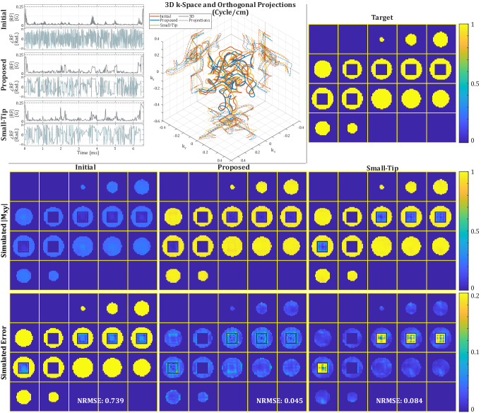
Figure S1: OV saturation pulses (and results) for the cuboid IV, designed with our approach (Proposed) and Sun’s small-tip method (experiment OV90 in the main manuscript). On the 3D k-space plot, the three trajectories explore largely overlapping regions in excitation k-space. Our approach has much smaller (-46%) NRMSE in simulation compared to Small-Tip. Small-Tip approach has larger error inside the IV: This is expected, as the method produces only small-tip pulses, that we then scaled to meet the large-tip objective. The scaling increases excitation error inside IV while reducing error in the OV. Our approach directly designs large-tip pulses without this type of ‘scaling’ error.

A-B IV180

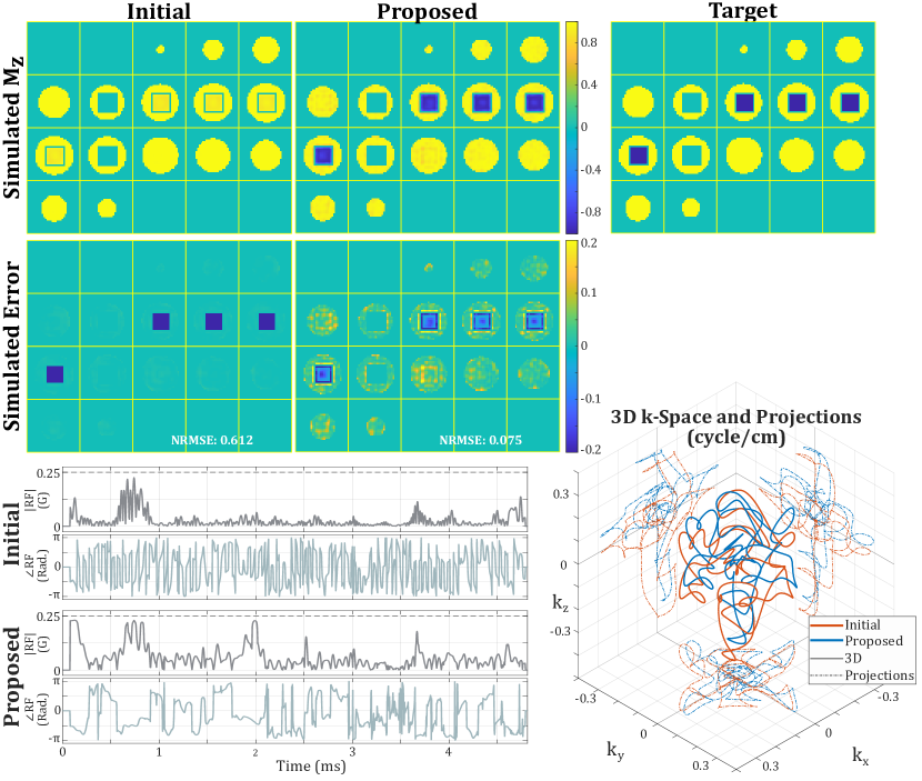
Figure S2: Cuboid IV inversion (experiment IV180 in the main manuscript). The lower left panel compares the RF waveforms of the initial and optimized (Proposed) pulses. The lower right panel compares the k-space trajectories of the two pulses.

A-C IV180M

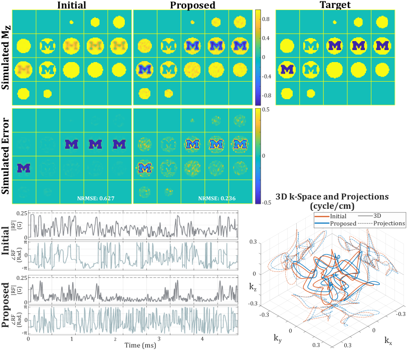
Figure S3: Block-M IV inversion pulse (experiment IV180M in the main manuscript). The lower left panel compares the RF waveforms of the initial and optimized (Proposed) pulses. The lower right panel compares the k-space trajectories of the two pulses.

A-D Brain Simulation

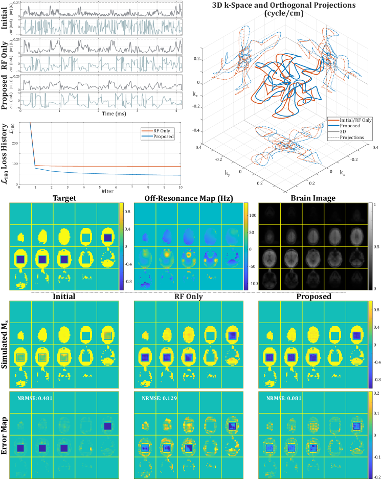
Figure S4: Cuboid IV inversion based on a B0 (off-resonance) map obtained in a volunteer. Three pulses are compared: (1) Initial, (2) ’RF Only’, obtained by keeping the gradients fixed at their initial shapes and optimizing only the RF waveform with the proposed auto-differentiation approach, and (3) the proposed jointly optimized pulse. While our optimized k-space trajectory is similar to the initial k-space trajectory, the jointly optimized pulse (Proposed) attains an excitation accuracy (NRMSE: 8.1%) that is 37% better than the ’RF Only’ pulse (NRMSE: 12.9%). This improvement is also reflected in the convergence ($\mathcal{L}_{180}$ loss history) plot.

Appendix B Unnormalized Inversion Images

In Fig. S5, we show the unnormalized images for the 3D spatially tailored inversion experiments (IV180, IV180M). In the main text, we normalized the “Cuboidal” and “Block-M” images by element-wise division by the “No Inversion” image, which eliminates the image intensity and phase variations due to receiver coil sensitivity.

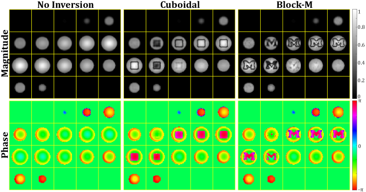
Figure S5: Images from the IV180 and IV180M experiments. “Cuboidal” and “Block-M” are the raw images of the IV180 and IV180M experiments, respectively. “No Inversion” was acquired using the same sequence (TR/TE, flip-angle, readout trajectory), except the inversion pulse in the sequence has RF amplitude set to 0. The 3 sets of magnitude and phase images shown here share the same image intensity and phase variations due to receiver coil sensitivity.

Appendix C Alternating vs Simultaneous Minimization

Here we compare the alternating optimization used in the main text with a simultaneous update scheme that optimizes $b$ (RF waveform) and $g$ (the three gradient waveforms) together at each iteration rather than fixing one and optimizing the other. We observe empirically that for the $\mathcal{L}_{90}$ and $\mathcal{L}_{180}$ losses defined in the main text, with extended kt-points initializations, the alternating update decreases the design losses faster than the simultaneous update. However, the two objectives are both non-convex in terms of $b$ and $g$, which makes this behavior difficult to analyze. We therefore cannot claim that this alternating scheme will outperform simultaneous updates in the general case (i.e., for all other design problems).

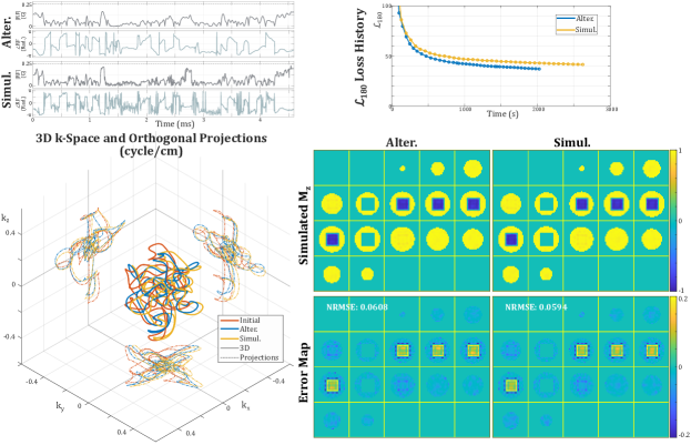
Figure S7: Same comparison as in Fig. S6, for the IV180 design. The simultaneous approach attains a slightly better inversion, but ends with a higher loss value (likely due to the RF power penalization term).

Appendix D Impact of a Small Gradient Delay

On modern MRI scanners, the physically realized gradient waveforms are typically slightly misaligned in time relative to the RF waveform, even after the vendor’s built-in gradient delay correction is applied. This delay is on the order of the gradient sampling (dwell, or raster) time, which on our scanner is $4\text{\,}\mathrm{\SIUnitSymbolMicro s}$. To assess robustness against such delays, we simulated the excitation produced by the OV90 and IV180 pulses for delays of $4\text{\,}\mathrm{\SIUnitSymbolMicro s}$ and $-4\text{\,}\mathrm{\SIUnitSymbolMicro s}$. As shown in Fig. S8, such delays led to excitation patterns that are visually nearly indistinguishable from the original patterns with no delay, and degraded the performance of our designed pulses by less than $1$ percentage point in NRMSE.

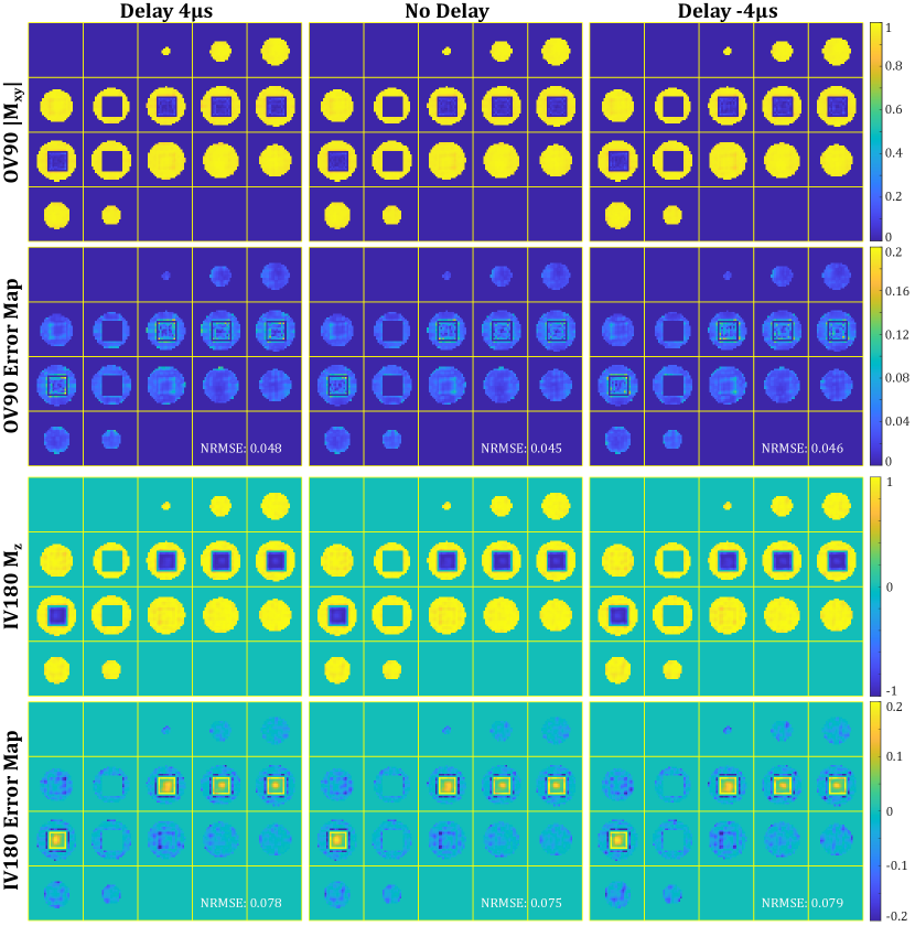
Figure S8: Simulated excitation performances of our designed OV90 and IV180 pulses under different delays of the applied gradient fields.

Appendix E Impact of Incorrect Off-Resonance

Motion or respiratory effects can cause mismatch between the acquired and actual off-resonance patterns. To assess robustness against such mismatch, we simulated the excitation produced by the same OV90 and IV180 pulses under different off-resonance maps: (i) the acquired off-resonance map, and (ii) the acquired off-resonance map scaled by a multiplicative factor of 3. As shown in Fig. S9, such mismatch led to a very similar excited patterns with about $1$ percentage point increases in NRMSE.

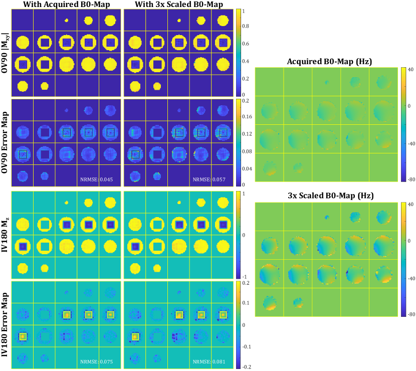
Figure S9: Simulated excitation performances of our designed OV90 and IV180 pulses under different off-resonance maps.

References

- [1] J. Pauly, D. Nishimura, and A. Macovski, “A k-space analysis of small-tip-angle excitation,” Journal of Magnetic Resonance, vol. 81, no. 1, pp. 43–56, jan 1989.
- [2] C. Ma, D. Xu, K. F. King, and Z.-P. Liang, “Joint design of spoke trajectories and RF pulses for parallel excitation,” Magnetic Resonance in Medicine, vol. 65, no. 4, pp. 973–985, apr 2011. [Online]. Available: http://doi.wiley.com/10.1002/mrm.22676
- [3] A. Zelinski, L. L. Wald, K. Setsompop, V. Goyal, and E. Adalsteinsson, “Sparsity-Enforced Slice-Selective MRI RF Excitation Pulse Design,” IEEE Transactions on Medical Imaging, vol. 27, no. 9, pp. 1213–1229, sep 2008.
- [4] M. A. Cloos et al., “kT-points: Short three-dimensional tailored RF pulses for flip-angle homogenization over an extended volume,” Magnetic Resonance in Medicine, vol. 67, no. 1, pp. 72–80, jan 2012. [Online]. Available: http://doi.wiley.com/10.1002/mrm.22978
- [5] D. Yoon, J. A. Fessler, A. C. Gilbert, and D. C. Noll, “Fast joint design method for parallel excitation radiofrequency pulse and gradient waveforms considering off-resonance,” Magnetic Resonance in Medicine, vol. 68, no. 1, pp. 278–285, jul 2012. [Online]. Available: http://doi.wiley.com/10.1002/mrm.24311
- [6] W. A. Grissom, M.-M. Khalighi, L. I. Sacolick, B. K. Rutt, and M. W. Vogel, “Small-tip-angle spokes pulse design using interleaved greedy and local optimization methods,” Magnetic Resonance in Medicine, vol. 68, no. 5, pp. 1553–1562, nov 2012. [Online]. Available: http://doi.wiley.com/10.1002/mrm.24165
- [7] C.-Y. Yip, W. A. Grissom, J. A. Fessler, and D. C. Noll, “Joint design of trajectory and RF pulses for parallel excitation,” Magnetic Resonance in Medicine, vol. 58, no. 3, pp. 598–604, sep 2007.
- [8] C. J. Hardy, P. A. Bottomley, M. O’Donnell, and P. B. Roemer, “Optimization of two-dimensional spatially selective NMR pulses by simulated annealing,” Journal of Magnetic Resonance, vol. 77, no. 2, pp. 233–250, 1988.
- [9] M. Davids, L. R. Schad, L. L. Wald, and B. Guérin, “Fast three-dimensional inner volume excitations using parallel transmission and optimized k-space trajectories,” Magnetic Resonance in Medicine, vol. 76, no. 4, pp. 1170–1182, oct 2016. [Online]. Available: http://doi.wiley.com/10.1002/mrm.26021
- [10] S. Tingting, X. Ling, T. Guisheng, C. Jieru, L. Feng, and S. Crozier, “Advanced Three-Dimensional Tailored RF Pulse Design in Volume Selective Parallel Excitation,” IEEE Transactions on Medical Imaging, vol. 31, no. 5, pp. 997–1007, may 2012. [Online]. Available: http://ieeexplore.ieee.org/document/6094221/
- [11] S. J. Malik, S. Keihaninejad, A. Hammers, and J. V. Hajnal, “Tailored excitation in 3D with spiral nonselective (SPINS) RF pulses,” Magnetic Resonance in Medicine, vol. 67, no. 5, pp. 1303–1315, may 2012. [Online]. Available: http://doi.wiley.com/10.1002/mrm.23118
- [12] H. Sun, J. A. Fessler, D. C. Noll, and J.-F. Nielsen, “Joint Design of Excitation k-Space Trajectory and RF Pulse for Small-Tip 3D Tailored Excitation in MRI,” IEEE Transactions on Medical Imaging, vol. 35, no. 2, pp. 468–479, feb 2016. [Online]. Available: http://ieeexplore.ieee.org/document/7268765/
- [13] H. Sun, “Topics in steady-state MRI sequences and RF pulse optimization,” Ph.D. dissertation, University of Michigan, Ann Arbor, 2015.
- [14] K. Setsompop, L. L. Wald, V. Alagappan, B. A. Gagoski, and E. Adalsteinsson, “Magnitude least squares optimization for parallel radio frequency excitation design demonstrated at 7 Tesla with eight channels,” Magnetic Resonance in Medicine, vol. 59, no. 4, pp. 908–915, apr 2008. [Online]. Available: http://doi.wiley.com/10.1002/mrm.21513
- [15] A. Paszke et al., “Automatic differentiation in pytorch,” in NIPS Autodiff Workshop, 2017.
- [16] F. H. Clarke, “Nonsmooth analysis and optimization,” in Proceedings of the international congress of mathematicians, vol. 5, 1983, pp. 847–853.
- [17] A. Griewank and A. Walther, Evaluating Derivatives: Principles and Techniques of Algorithmic Differentiation. Society for Industrial and Applied Mathematics, jan 2008. [Online]. Available: https://doi.org/10.1137%2F1.9780898717761
- [18] F. S. Sisser, “Elimination of bounds in optimization problems by transforming variables,” Mathematical Programming, vol. 20, no. 1, pp. 110–21, Dec. 1981.
- [19] S. Boyd and L. Vandenberghe, Convex Optimization. Cambridge University Press, 2004.
- [20] T. Luo, D. C. Noll, and J.-f. Nielsen, “3d inner volume imaging with 3d tailored outer volume suppression rf pulses,” in ISMRM, 2019, p. 4631. [Online]. Available: http://archive.ismrm.org/2019/4631.html
- [21] D. Mitsouras, R. V. Mulkern, and F. J. Rybicki, “Strategies for inner volume 3d fast spin echo magnetic resonance imaging using nonselective refocusing radio frequency pulsesa),” Medical Physics, vol. 33, no. 1, pp. 173–186, 2005.
- [22] B. Wilm, J. Svensson, A. Henning, K. Pruessmann, P. Boesiger, and S. Kollias, “Reduced field-of-view mri using outer volume suppression for spinal cord diffusion imaging,” Magnetic Resonance in Medicine, vol. 57, no. 3, pp. 625–630, 2007.
- [23] C.-y. Yip, J. A. Fessler, and D. C. Noll, “Iterative RF pulse design for multidimensional, small-tip-angle selective excitation,” Magnetic Resonance in Medicine, vol. 54, no. 4, pp. 908–917, oct 2005. [Online]. Available: http://doi.wiley.com/10.1002/mrm.20631
- [24] J.-F. Nielsen and D. C. Noll, “Toppe: A framework for rapid prototyping of mr pulse sequences,” Magnetic Resonance in Medicine, vol. 79, no. 6, pp. 3128–3134, 2018. [Online]. Available: https://onlinelibrary.wiley.com/doi/abs/10.1002/mrm.26990
- [25] K. J. Layton et al., “Pulseq: A rapid and hardware-independent pulse sequence prototyping framework,” Mag. Res. Med., vol. 77, no. 4, pp. 1544–52, Apr. 2017.
- [26] S. M. Conolly, D. G. Nishimura, A. Macovski, and G. Glover, “Variable-rate selective excitation,” Journal of Magnetic Resonance, vol. 78, no. 3, pp. 440 – 458, 1988.
- [27] T. Luo, D. C. Noll, J. A. Fessler, and J.-F. Nielsen, “Multi-scale accelerated auto-differentiable bloch-simulation based joint design of excitation rf and gradient waveforms,” in ISMRM, 2021, p. 3958.
- [28] W. A. Grissom, K. Setsompop, S. A. Hurley, J. Tsao, J. V. Velikina, and A. A. Samsonov, “Advancing rf pulse design using an open-competition format: Report from the 2015 ismrm challenge,” Magnetic Resonance in Medicine, vol. 78, no. 4, pp. 1352–1361, 2017. [Online]. Available: https://onlinelibrary.wiley.com/doi/abs/10.1002/mrm.26512
- [29] B. A. Hargreaves, C. H. Cunningham, D. G. Nishimura, and S. M. Conolly, “Variable-rate selective excitation for rapid mri sequences,” Magnetic Resonance in Medicine, vol. 52, no. 3, pp. 590–597, 2004.
- [30] Z. Cao, M. J. Donahue, J. Ma, and W. A. Grissom, “Joint design of large-tip-angle parallel RF pulses and blipped gradient trajectories,” Magnetic Resonance in Medicine, vol. 75, no. 3, pp. 1198–1208, 2016.
- [31] S. M. Conolly, D. G. Nishimura, and A. Macovski, “Optimal Control Solutions to the Magnetic Resonance Selective Excitation Problem,” IEEE Transactions on Medical Imaging, vol. 5, no. 2, pp. 106–115, jun 1986. [Online]. Available: http://ieeexplore.ieee.org/document/4307754/
- [32] W. A. Grissom, D. Xu, A. Kerr, J. A. Fessler, and D. C. Noll, “Fast Large-Tip-Angle Multidimensional and Parallel RF Pulse Design in MRI,” IEEE Transactions on Medical Imaging, vol. 28, no. 10, pp. 1548–1559, oct 2009. [Online]. Available: http://ieeexplore.ieee.org/document/4915785/