A purely hyperbolic discontinuous Galerkin approach for self-gravitating gas dynamics

Abstract

One of the challenges when simulating astrophysical flows with self-gravity is to compute the gravitational forces. In contrast to the hyperbolic hydrodynamic equations, the gravity field is described by an elliptic Poisson equation. We present a purely hyperbolic approach by reformulating the elliptic problem into a hyperbolic diffusion problem, which is solved in pseudotime, using the same explicit high-order discontinuous Galerkin method we use for the flow solution. The flow and the gravity solvers operate on a joint hierarchical Cartesian mesh and are two-way coupled via the source terms. A key benefit of our approach is that it allows the reuse of existing explicit hyperbolic solvers without modifications, while retaining their advanced features such as non-conforming and solution-adaptive grids. By updating the gravitational field in each Runge-Kutta stage of the hydrodynamics solver, high-order convergence is achieved even in coupled multi-physics simulations. After verifying the expected order of convergence for single-physics and multi-physics setups, we validate our approach by a simulation of the Jeans gravitational instability. Furthermore, we demonstrate the full capabilities of our numerical framework by computing a self-gravitating Sedov blast with shock capturing in the flow solver and adaptive mesh refinement for the entire coupled system.

1 Introduction

Numerical simulations of self-gravitating gas dynamics have become an indispensable tool in the investigation of astrophysical fluid dynamics, as evidenced by the multitude of publicly available simulation codes [1, 2, 3, 4, 5, 6, 7]. The gravitational effect of matter on itself and its surroundings plays an important role in many such flow problems, e.g., for cosmological structure formation [8, 9], core-collapse supernovae [10], or star formation [11, 12]. In non-relativistic simulations, self-gravity is modelled by a Poisson equation for the Newtonian gravitational potential $\phi$,

$$-\vec{\nabla}^{2}\phi=-4\pi G\rho,$$ (1.1)

where $G$ is the universal gravitational constant and $\rho$ is the mass density. A particular challenge for simulating self-gravity is that (1.1) is of elliptic type, i.e., the solution at each point in space depends on the solution at all other points simultaneously. So, typically, alternative solution methods than those employed for the hyperbolic hydrodynamics equations are required. Examples are multigrid methods [13], multipole expansion [10], or tree-based algorithms [14, 15]. Some commonalities of these methods are their computational expense and that they can be difficult to parallelize due to the global nature of the problem statement.

In 2007, Nishikawa [16] introduced a new strategy for determining the steady-state solution to the diffusion equation by rewriting it as a first-order hyperbolic system (FOHS) with a relaxation time. He noted that when all derivatives with respect to time become zero, the FOHS reduces to an elliptic equation. Thus, by relaxing the FOHS to steady state, it is possible to recover the solution for Laplace- and Poisson-type equations.

Based on this analysis, we present a new numerical approach for self-gravitating gas dynamics, where we follow Nishikawa’s ansatz and reformulate (1.1) as a first-order hyperbolic system. That is, we determine the gravitational potential of a given density distribution as the steady-state solution to a FOHS with the appropriate Poisson source term of (1.1). A key benefit of this strategy is that it allows us to use the same explicit discontinuous Galerkin scheme for both gravity and gas dynamics, yielding a comparatively simple high-order multi-physics approach for hydrodynamics with self-gravity. Instead of requiring special treatment of the elliptic equation for gravity, it is sufficient to set up a hyperbolic solver for each physical system, which are coupled via the respective source terms. As an additional advantage, this approach enables us to exploit advanced features of existing solvers for hyperbolic equations without further modifications, such as local mesh refinement and solution-adaptive grids.

In Nishikawa’s original paper [16], he reformulated the diffusion equation,

$$u_{t}-\nu\vec{\nabla}^{2}u=0,$$ (1.2)

as the first-order hyperbolic system,

$$u_{t}-\nu(q_{1,x}+q_{2,y}) =0,$$ (1.3)

$$q_{1,t}-\frac{u_{x}}{T_{r}} =-\frac{q_{1}}{T_{r}},$$

$$q_{2,t}-\frac{u_{y}}{T_{r}} =-\frac{q_{2}}{T_{r}}.$$

Here, $\nu$ is the diffusion coefficient, $T_{r}$ is the relaxation time, and $q_{1},q_{2}$ are auxiliary variables. The first approach to rewrite (1.2) as a hyperbolic problem dates back to 1958, when Cattaneo [17] introduced the hyperbolic heat equations. Later, Nagy et al. [18] showed that solutions of (1.3) converge uniformly to solutions of (1.2) as $T_{r}$ goes to zero. However, the system (1.3) becomes stiff for very small values of $T_{r}$ and, thus, prohibitively expensive to solve with an explicit time integration scheme. Implicit schemes, on the other hand, are generally more difficult to parallelize and can suffer from reduced solution accuracy due to the stiff source term [19].

It was Nishikawa who realized that the key property of (1.3) is that it is equivalent to the original equation (1.2) at the steady state for any value of $T_{r}$ [16], thereby avoiding the stiffness problem. That is, if all derivatives with respect to time are zero, we obtain

$$\left.\begin{aligned} -\nu(q_{1,x}+q_{2,y})&=0\\ u_{x}&=q_{1}\\ u_{y}&=q_{2}\\ \end{aligned}\,\right\}\quad\to\quad-\nu\vec{\nabla}^{2}u=0.$$ (1.4)

Thus by solving the hyperbolic system (1.3) to steady state, we can obtain the solution to an elliptic problem at arbitrary precision. This idea has been successfully applied to develop finite volume-type methods, e.g., [20, 21, 22, 23], as well as discontinuous Galerkin-type methods, e.g., [24, 25], that approximate the solution of parabolic partial differential equations.

Other attempts to reformulate the Poisson equation for gravity to reduce the associated computational complexity have been made. Black and Bodenheimer [26] recast the elliptic equation as a parabolic equation to solve it iteratively to steady state with an alternating-direction implicit scheme [27]. While this approach has been implemented successfully [28, 29, 1], it still requires a specialized solver for the gravitational potential. Hirai et al. [30] proposed to rewrite (1.1) as an inhomogeneous wave equation, motivated by the hyperbolicity of general relativity. Their hyperbolic system recovers Newtonian gravity in the limit of infinite propagation speed for gravitation, with all the associated issues of becoming a stiff problem. In practice, they found that the propagation speed can be taken relatively small without significantly degrading the solution, as long as it exceeds the characteristic velocity of the coupled flow problem. While their scheme is far more efficient than a direct Poisson solver, they also reported that the exact value for the propagation speed is problem-dependent and that the incurred modeling error strongly depends on the boundary conditions and domain size.

lne:intro_motive_start We note that restricting to the particular application of self-gravity multi-physics problems yields a slightly different mindset compared to the goal of developing a general Poisson-type solver. For instance, it is the case that one has a very good initial solution guess for the gravity system due to its gradual evolution with respect to the fluid density, and most self-gravity problems in practice require adaptive mesh refinement. It is within the purview of self-gravitating gas dynamics that we bring together ideas and apply a hyperbolic diffusion methodology to approximate the solution of a Poisson-type problem with a high-order discontinuous Galerkin method.

A principal goal of this work is to explore this hyperbolic gravity approach, in particular, if it retains the high-order accuracy of the underlying approximation and if it offers a viable alternative for self-gravitating applications. Additionally, we lne:intro_motive_end demonstrate that it is possible to reuse existing numerical tools for hyperbolic problems to compute the gravitational potential. For the flow field, the compressible Euler equations are discretized in space by a high-order discontinuous Galerkin method and integrated in time by an explicit Runge-Kutta scheme. The same numerical solver is also used to determine the gravitational field by advancing the corresponding FOHS to steady state. In a coupled simulation, the gravitational potential corresponding to the current density distribution is determined before each Runge-Kutta stage of the hydrodynamics solver. The resulting gravitational forces are then used in the source term during the subsequent Runge-Kutta stage of the flow solver. Both solvers operate on a shared hierarchical Cartesian mesh that can be adaptively refined to match dynamically changing resolution requirements. We verify the accuracy of the numerical methods by showing high-order convergence for the hydrodynamics and gravity solvers both in single-physics and multi-physics computations. In addition to a standard explicit Runge-Kutta scheme, we also discuss a Runge-Kutta scheme optimized for reaching the steady-state solution of the FOHS for the gravitational potential with a given spatial semi-discretization faster. The suitability of our approach for applied astrophysics problems is validated by performing coupled flow–gravity simulations of the Jeans gravitational instability and of a Sedov explosion with self-gravity. All results are obtained with the open-source simulation framework Trixi.jl [31], and the corresponding numerical setups are publicly available to facilitate reproducibility [32].

The manuscript is organized as follows: In the next section, we will introduce the governing equations for purely hyperbolic self-gravitational gas dynamics, present the used numerical methods and discuss how the coupling of gas dynamics and gravity is achieved. Results for the individual single-physics solvers and for fully coupled flow-gravity simulations are given in Section 3. Finally, in Section 4 we summarize our findings. Further details on the algorithmic and implementation details are provided in A.

2 Mathematical model and numerical methods

In this section, we introduce the governing equations for self-gravitating gas dynamics with the compressible Euler equations and show how to reformulate the Poisson equation for the gravity potential as a hyperbolic diffusion system. This is followed by an outline of the discontinuous Galerkin spectral element method (DGSEM) used for the spatial discretization. After, we present the employed time integration methods and discuss optimized schemes for the hyperbolic gravity system. Finally, we discuss how multi-physics coupling is achieved between the two hyperbolic solvers.

2.1 Governing equations for self-gravitating gas dynamics

In the following, we present the equations for compressible fluids under the influence of a gravitational potential. First, the compressible Euler equations are given in their standard form with source terms, proportional to the gravity potential, in the momenta and total energy [33]:

$$\frac{\partial}{\partial t}\begin{bmatrix}\rho\\[2.84544pt] \rho v_{1}\\[2.84544pt] \rho v_{2}\\[2.84544pt] E\\[2.84544pt] \end{bmatrix}+\frac{\partial}{\partial x}\begin{bmatrix}\rho v_{1}\\[2.84544pt] \rho v_{1}^{2}+p\\[2.84544pt] \rho v_{1}v_{2}\\[2.84544pt] (E+p)v_{1}\\[2.84544pt] \end{bmatrix}+\frac{\partial}{\partial y}\begin{bmatrix}\rho v_{2}\\[2.84544pt] \rho v_{1}v_{2}\\[2.84544pt] \rho v_{2}^{2}+p\\[2.84544pt] (E+p)v_{2}\\[2.84544pt] \end{bmatrix}=\begin{bmatrix}0\\[2.84544pt] -\rho\phi_{x}\\[2.84544pt] -\rho\phi_{y}\\[2.84544pt] -(\vec{v}\cdot\vec{\nabla}\phi)\rho\\[2.84544pt] \end{bmatrix}.$$ (2.1)

Here, $\rho$ is the density, $\vec{v}=(v_{1},v_{2})^{\mathsf{T}}$ are the velocities, and $E$ is the total energy. The pressure $p$ is determined from the ideal gas law

$$p=(\gamma-1)\left(E-\frac{\rho}{2}(v_{1}^{2}+v_{2}^{2})\right),$$ (2.2)

with the heat capacity ratio $\gamma$.

Following Nishikawa’s work [16], we convert the Poisson equation for the gravitational potential (1.1) into the hyperbolic gravity equations,

$$\frac{\partial}{\partial{{{\tau}}}}\begin{bmatrix}\phi\\[2.84544pt] q_{1}\\[2.84544pt] q_{2}\\[2.84544pt] \end{bmatrix}+\frac{\partial}{\partial x}\begin{bmatrix}-q_{1}\\[2.84544pt] -\phi/T_{r}\\[2.84544pt] 0\\[2.84544pt] \end{bmatrix}+\frac{\partial}{\partial y}\begin{bmatrix}-q_{2}\\[2.84544pt] 0\\[2.84544pt] -\phi/T_{r}\\[2.84544pt] \end{bmatrix}=\begin{bmatrix}-4\pi G\rho\\[2.84544pt] -q_{1}/T_{r}\\[2.84544pt] -q_{2}/T_{r}\\[2.84544pt] \end{bmatrix},$$ (2.3)

where $\tau$ is a pseudotime variable, lne:pseudotime_1 the auxiliary variables $(q_{1},q_{2})^{\mathsf{T}}\approx\vec{\nabla}\phi$ and $T_{r}$ is the relaxation time. For a general Poisson problem (with viscosity $\nu$), this relaxation time has the form

$$T_{r}=\frac{L_{r}^{2}}{\nu},$$ (2.4)

where $L_{r}$ is a reference length scale that can be freely chosen. For the gravitational potential equation (1.1) we have the diffusion constant $\nu=1$. lne:Lrscaling_start The work of Nishikawa [34] found that taking the length scale

$$L_{r}=\frac{1}{2\pi},$$ (2.5)

is optimal on unit square domains. Here, optimality is taken to be in the sense that the convergence of the hyperbolic system (2.3) to steady state is fastest. For the numerical results presented in Section 3, we found that (2.5) remained optimal on any square domain and, therefore, it is used throughout the present work. In more general rectangular or irregular domains, Nishikawa and Nakashima demonstrated that the reference length scaling $L_{r}$ must be adjusted to avoid erratic convergence behavior of the hyperbolic diffusion system lne:new_ref[35]. We note, however, that regardless of how one chooses $L_{r}$, lne:Lrscaling_end the steady-state solution of (2.3) is, in fact, the desired solution of the original Poisson problem (1.1) [16, 17, 36, 18].

In single-physics simulations of the compressible Euler equations or the hyperbolic gravity equations alone, the source terms in the governing equations are determined analytically. When considering coupled Euler-gravity problems, however, the gravity potential of the hyperbolic gravity system is used to generate the source term information in (2.1), while the density of the compressible Euler solution is used for the source term in (2.3). Thus, both systems of equations are connected via two-way coupling through their source terms.

2.2 High-order discontinuous Galerkin method on hierarchical Cartesian meshes

Next, we give an overview of the nodal discontinuous Galerkin spectral element method (DGSEM) on hierarchical Cartesian meshes. A full derivation can be found in, e.g., [37, 38, 39]. We consider the solution of systems of hyperbolic conservation laws in two spatial dimensions, which take the general form

$$\bm{u}_{t}+\vec{\nabla}\cdot\overset{\text{\tiny$\leftrightarrow$}}{\bm{f}}(\bm{u})=\bm{s}(\bm{u}),\qquad\forall\vec{x}\in\Omega,$$ (2.6)

on a square domain $\Omega$. Here $\bm{u}\in\mathbb{R}^{m}$, where $m$ is the number of equations, is the state vector of conserved variables, $\overset{\text{\tiny$\leftrightarrow$}}{\bm{f}}=(\bm{f}_{1},\bm{f}_{2})^{\mathsf{T}}$ is the block vector of the nonlinear fluxes, and $\bm{s}$ denotes a—possibly zero-valued—source term. We subdivide the domain $\Omega$ into $K$ non-overlapping square elements lne:mapping_start

$$E_{k}=\left[x_{k,1},x_{k,2}\right]\times[y_{k,1},y_{k,2}],\quad k=1,\ldots,K,$$ (2.7)

and we define $h:=\Delta x=\Delta y$ as the length of the respective Cartesian element. We transform between the reference element $E_{0}=[-1,1]^{2}$ and each element, $E_{k}$, from the mappings

$$X_{k}(\xi)=x_{k,1}+\frac{\xi+1}{2}h,\quad Y_{k}(\eta)=y_{k,1}+\frac{\eta+1}{2}h,\quad k=1,\ldots,K$$ (2.8)

with reference coordinates $\vec{\xi}=(\xi,\eta)^{\mathsf{T}}$. Under these mappings (2.8), the conservation law in physical coordinates (2.6) becomes a conservation law in reference coordinates

$$\frac{h^{2}}{4}\bm{u}_{t}+\frac{h}{2}\vec{\nabla}_{\xi}\cdot\overset{\text{\tiny$\leftrightarrow$}}{\bm{f}}=\frac{h^{2}}{4}\bm{s}(\bm{u}).$$ (2.9)

We simplify the conservation law in reference coordinates to be lne:mapping_end

$$J\bm{u}_{t}+\vec{\nabla}_{\xi}\cdot{\overset{\text{\tiny$\leftrightarrow$}}{\bm{f}}}=J\bm{s},$$ (2.10)

where $J=h/2$ is the one-dimensional Jacobian determinant.

The starting point of the DGSEM is the weak form of the conservation law, for which we multiply (2.10) by an appropriate test function $\varphi\in L_{2}(\Omega)$ and integrate over the reference element. After integration-by-parts, we obtain the weak form

$$\int\limits_{{E_{0}}}J\bm{u}_{t}\varphi\,\mathrm{d}\vec{\xi}+\int\limits_{\partial{E_{0}}}(\overset{\text{\tiny$\leftrightarrow$}}{\bm{f}}\cdot\vec{n})\varphi\,\mathrm{d}S-\int\limits_{{E_{0}}}\overset{\text{\tiny$\leftrightarrow$}}{\bm{f}}\cdot\vec{\nabla}_{\xi}\varphi\,\mathrm{d}\vec{\xi}=\int\limits_{{E_{0}}}J\bm{s}\varphi\,\mathrm{d}\vec{\xi},$$ (2.11)

where $\vec{n}$ is the outer unit normal at the boundary $\partial{E_{0}}$. We approximate each component of the state vector by polynomials of degree $N$ in each spatial dimension, which we represent as $\bm{U}$. The polynomials are written in terms of the Lagrange basis $\psi_{ij}(\,\vec{\xi}\,)=l_{i}(\xi)l_{j}(\eta)$, $i,j=0,\ldots,N$, where the interpolation nodes are the Legendre-Gauss-Lobatto (LGL) points. Lagrange polynomials of degree $N$ are also used to approximate the fluxes $\overset{\text{\tiny$\leftrightarrow$}}{\bm{F}}=(\bm{F}_{1},\bm{F}_{2})^{\mathsf{T}}$ and source terms $\bm{S}$. Integrals in (2.11) are evaluated discretely by LGL quadrature such that the interpolation and quadrature nodes are collocated. To resolve the solution discontinuity at element interfaces, we replace the boundary fluxes by numerical fluxes $\bm{F}_{n}^{*}\approx\overset{\text{\tiny$\leftrightarrow$}}{\bm{F}}\cdot\vec{n}$, see, e.g., [37]. In this work, we use the Harten, Lax, van Leer (HLL) flux [40, 41] for the compressible Euler system and the local Lax-Friedrichs (LLF) flux [41, 24] for hyperbolic gravity. We choose the tensor product basis $\varphi\in\{\psi_{ij}\}_{i,j=0}^{N}$ to be the $(N+1)^{2}$ test functions. The final weak form of (2.6) in the standard DGSEM formulation then reads

$$\int\limits_{{E_{0}},N}J\bm{U}_{t}\psi_{ij}\,\mathrm{d}\vec{\xi}+\int\limits_{\partial{E_{0}},N}\bm{F}_{n}^{*}\psi_{ij}\,\mathrm{d}S-\int\limits_{{E_{0}},N}\overset{\text{\tiny$\leftrightarrow$}}{\bm{F}}\cdot\vec{\nabla}_{\xi}\psi_{ij}\,\mathrm{d}\vec{\xi}=\int\limits_{{E_{0}},N}J\bm{S}\psi_{ij}\,\mathrm{d}\vec{\xi},\qquad\forall i,j=0,\ldots,N.$$ (2.12)

Inserting the definitions for the approximate solution, fluxes, and source terms, we obtain the semi-discrete DG operator, which is integrated in time with an explicit Runge-Kutta scheme. The stable time step is calculated by

$$\Delta t=\frac{\mathtt{CFL}}{N+1}\frac{h}{\Lambda},$$ (2.13)

where $\Lambda_{\mathrm{Eu}}=\max(\mathopen{|}\vec{v}\mathclose{|}+c)$ with the speed of sound $c=\sqrt{\gamma p/\rho}$ for the compressible Euler system and $\Lambda_{\mathrm{Gr}}=\sqrt{\nu/T_{r}}$ for the gravity system. Suitable time integration schemes will be discussed in the next section.

An alternative split-form DGSEM approximation can be obtained by making use of the summation-by-parts (SBP) property inherent to the nodal DG scheme on LGL nodes [42]. Applying summation-by-parts once more to (2.12) produces the strong form of the conservation law (2.10). Following the work of Fisher et al. and Carpenter et al. [43, 44], we introduce a numerical volume flux for the flux derivative. This yields a split-form DG approximation [45, 46], which allows to use symmetric two-point flux functions with additional desirable properties such as entropy conservation or kinetic energy preservation [47, 48, 49, 50]. Here, we select the numerical flux of Chandrashekar [51].

The split-form variant is also the basis for the high-order shock capturing approach by Hennemann et al. [52], which we utilize in the DG solver for simulating compressible Euler problems with strong discontinuities. In this approach, each DG element is divided into $(N+1)^{2}$ subcells, on which a first-order finite volume (FV) method is used to obtain the semi-discrete operator. The final operator is then obtained by blending the DG operator in each element with the FV operator based on the energy content in the highest modes, while retaining the discrete entropic property.

To support non-conforming elements created by local mesh refinement, we employ the mortar method [53, 54]. In this approach, mortar surfaces are inserted at interfaces with a coarse element adjacent to multiple refined elements, see Fig. 1(a). The solution values at non-conforming element interfaces are interpolated to the mortar, where the surface flux is calculated at conforming node locations. Then, the flux values are discretely projected back to the non-conforming element interfaces. A similar approach is used for adaptive mesh refinement (AMR), see Fig. 1(b). During refinement, the solution on the coarse element is interpolated to the LGL nodes on the four refined elements. Conversely, during coarsening the solution on the four refined elements is projected onto the coarse element. These AMR procedures in two dimensions correspond exactly to the algorithms used for a mortar element approach in three dimensions [55]. Therefore, both the mortar method and the AMR technique are fully conservative. A detailed derivation of the DGSEM on non-conforming hierarchical Cartesian meshes can be found in, e.g., [39].

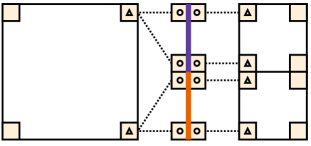
(a) Mortar method: non-conforming nodes on element surfaces (square with triangle) become conforming nodes on mortar elements (square with circle).

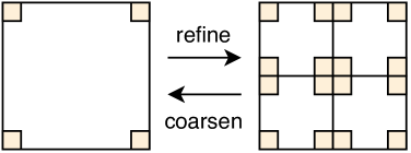
(b) Adaptive mesh refinement: solution transfer between coarse and refined cells.

Figure 1: Illustration of the mortar element method and transfer operators for adaptive mesh refinement.

2.3 Time integration schemes

For the compressible Euler solver, we use the fourth-order, five-stage low-storage scheme CK45 by Carpenter and Kennedy [56] with CFL-based step size control (2.13). This and other common time integration methods can also be used to advance the hyperbolic diffusion part to steady state. To improve the performance of integration in pseudotime [57] and reduce the sensitivity to user-chosen parameters [58], locally adaptive error-based time step control could be employed and the Runge-Kutta schemes can be optimized for the given spatial semi-discretizations to be able to take bigger time steps [59].

Here, we briefly demonstrate the last approach. lne:timestep_opt_start The motivation behind this strategy is to grant the scheme an ability to take larger explicit time steps, which leads to faster steady state convergence for the numerical examples considered in Section 3. lne:timestep_opt_end Following [60], we computed the spectrum of the standard DG operator using a local Lax-Friedrichs interface flux and polynomials of degree $N=3$ for the hyperbolic diffusion problem (1.3). The convex hull of this spectrum was used as input to optimize the stability polynomial of an explicit, second-order accurate five-stage Runge-Kutta method using the algorithm of [61]. Finally, a low-storage scheme of the 3S* class [62] was constructed by minimizing the principal truncation error, given the optimized stability polynomial as constraint. For this, we used the algorithms implemented in RK-Opt [63], which are based on MATLAB [64]. We used NodePy [65] to verify the desired properties of the resulting five-stage second-order method RK3S* with low-storage coefficients listed in Table 1. The minimum-storage implementation [62] is shown in Algorithm 1. Applying RK3S* instead of CK45 increases the performance and does not influence the accuracy negatively, as shown in Sections 3.1.3 and 3.2.1 below. We also optimized first- and third-order accurate schemes analogously but these did not improve performance as much, e.g., for the test described in Section 3.2.1.

Table 1: Minimum-storage coefficients [62] of the second-order accurate explicit low-storage Runge-Kutta method RK3S* optimized for hyperbolic diffusion.

$i$	$\gamma_{1,i}$	$\gamma_{2,i}$	$\gamma_{3,i}$
1	0.0000000000000000E+00	1.0000000000000000E+00	0.0000000000000000E+00
2	5.2656474556752575E-01	4.1892580153419307E-01	0.0000000000000000E+00
3	1.0385212774098265E+00	-2.7595818152587825E-02	0.0000000000000000E+00
4	3.6859755007388034E-01	9.1271323651988631E-02	4.1301005663300466E-01
5	-6.3350615190506088E-01	6.8495995159465062E-01	-5.4537881202277507E-03
$i$	$\delta_{i}$	$\beta_{i}$	$c_{i}$
1	1.0000000000000000E+00	4.5158640252832094E-01	0.0000000000000000E+00
2	1.3011720142005145E-01	7.5974836561844006E-01	4.5158640252832094E-01
3	2.6579275844515687E-01	3.7561630338850771E-01	1.0221535725056414E+00
4	9.9687218193685878E-01	2.9356700007428856E-02	1.4280257701954349E+00
5	0.0000000000000000E+00	2.5205285143494666E-01	7.1581334196229851E-01

$S_{1}\leftarrow u^{n},S_{2}\leftarrow 0,S_{3}\leftarrow u^{n}$

for all $i\in\{1,\dots,s\}$ do

    $S_{2}\leftarrow S_{2}+\delta_{i}S_{1}$

    $S_{1}\leftarrow\gamma_{1,i}S_{1}+\gamma_{2,i}S_{2}+\gamma_{3,i}S_{3}+\beta_{i}\Delta tf(t_{n}+c_{i}\Delta t,S_{1})$

end for

$u^{n+1}\leftarrow S_{1}$

Algorithm 1 Minimum-storage implementation of one step of a 3S* method with $s$ stages applied to the ODE $u_{t}(t)=f(t,u(t))$.

2.4 Multi-physics coupling

The results presented in Section 3 were obtained with Trixi.jl [31], an open-source numerical simulation framework for hyperbolic conservation laws developed by the authors. Trixi.jl is based on a modular architecture, where all components are only loosely coupled with each other such that it is easy to extend or replace existing functionality.

lne:multiphys_start A complete description of the control flow and algorithmic structure of Trixi.jl for single-physics simulation setups on hierarchical Cartesian meshes is provided in A. The extension to a coupled flow-gravity simulation is straightforward, since the compressible Euler hydrodynamic solver and the hyperbolic gravity solver both use a high-order DG spatial approximation. Therefore, one can instantiate two instances of the DG solver that operate on the same quadtree mesh. We note that only the solution information from the compressible Euler equations is used to control the quadtree mesh and its possible adaptation via AMR (see A for details). The gravity solver, however, is passively adapted to match the new quadtree mesh such that both solvers continue to use the same spatial discretization. We highlight the ease with which one can adapt to multi-physics simulations is due to the treatment of the gravity equations in a hyperbolic fashion and the ability to directly reuse tools from an existing single-physics DG architecture to approximate the solution of the gravity potential and its derivatives (2.3).

The key component of the multi-physics simulation is the exchange of information between the hydrodynamics and hyperbolic gravity solvers via their source terms. This coupling introduces a crucial algorithmic choice within the time integration loop of the hydrodynamics solver. One can choose to evolve the hyperbolic gravity variables to steady state in pseudotime either within every stage of the Runge-Kutta scheme of the hydrodynamics solver (left part of Fig. 2) or once every Runge-Kutta time step of the hydrodynamics solver (right part of Fig. 2). This choice impacts the overall solution accuracy as we demonstrate with results given in Sections 3.1.3 and 3.2.1. lne:multiphys_end

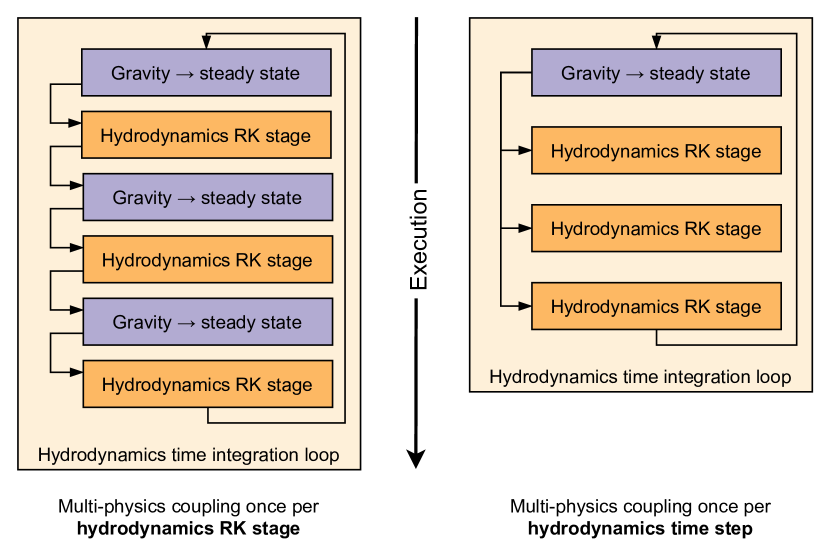
Figure 2: (left) Flowchart for a flow-gravity simulation with coupling once per Runge-Kutta (RK) stage of the hydrodynamics solver (right) Flowchart for a flow-gravity simulation with coupling once per time step of the hydrodynamics solver.

lne:new_algs_start In Algorithms 2 and 3 we provide pseudocode for these two coupling strategies. With either coupling variant, we insert a pseudotime integration loop to evolve the hyperbolic gravity solution variables to a new steady state into the time integration loop of the hydrodynamics solver. As discussed in Section 2.3, the time integration scheme for the gravity system can differ from the time integration scheme of the hydrodynamics system. For the integration in pseudotime, the previous gravity solution is used as the initial guess, lne:new_algs_end and the source terms as given in (2.3) are determined from the density field of the hydrodynamics solver. After the gravity field is converged to steady state according to the specified residual threshold, the compressible Euler solver is executed accordingly, with the source terms as given in (2.1) computed from the solution of the gravity solver. As a final note, since both solvers operate on the same mesh with the same polynomial order, no interpolation is required between the hydrodynamics and gravity solutions.

while $t<t_{\text{final}}$  do

    $\Delta t_{\text{Euler}}\leftarrow$ Value from (2.13) for hydrodynamics solver

    for all $i\in\{1,\dots,s\}$ do

         $t_{\text{stage}}\leftarrow t+c_{i}\Delta t_{\text{Euler}}$

         while $\phi_{\tau}>\mathtt{tol}$ do // Gravity loop in pseudotime $\tau$

             $\Delta t_{\text{Gravity}}\leftarrow$ Value from (2.13) for hyperbolic gravity solver

             Update $\bm{u}_{\text{Gravity}}$ using density $\rho$ at $t_{\text{stage}}$ in (2.3) with gravity solver RK method

         end while

         Update $\bm{u}_{\text{Euler}}$ using $q_{1},q_{2}$ at $t_{\text{stage}}$ in (2.1) with hydrodynamics solver RK method

    end for

    $t\leftarrow t+\Delta t_{\text{Euler}}$

end while

Algorithm 2 Procedure to couple and update hyperbolic gravity variables once every Runge-Kutta stage in the compressible Euler time integration loop.

while $t<t_{\text{final}}$  do

    while $\phi_{\tau}>\mathtt{tol}$ do // Gravity loop in pseudotime $\tau$

         $\Delta t_{\text{Gravity}}\leftarrow$ Value from (2.13) for hyperbolic gravity solver

         Update $\bm{u}_{\text{Gravity}}$ using density $\rho$ at current time $t$ in (2.3) with gravity solver RK method

    end while

    $\Delta t_{\text{Euler}}\leftarrow$ Value from (2.13) for hydrodynamics solver

    for all $i\in\{1,\dots,s\}$ do

         $t_{\text{stage}}\leftarrow t+c_{i}\Delta t_{\text{Euler}}$

         Update $\bm{u}_{\text{Euler}}$ using $q_{1},q_{2}$ at fixed $t$ in (2.1) with hydrodynamics solver RK method

    end for

    $t\leftarrow t+\Delta t_{\text{Euler}}$

end while

Algorithm 3 Procedure to couple and update hyperbolic gravity variables once every Runge-Kutta time step in the compressible Euler time integration loop.

3 Numerical results

In this section, we present numerical tests to verify and validate the multi-physics implementation of the DG solver in Trixi.jl [31]. We begin with a demonstration, in Section 3.1, of the high-order accuracy for both single- and multi-physics problems. Next, in Section 3.2, we simulate two example problems for compressible, self-gravitating flows. All parameter files required for reproducing the results are also available online [32].

The time integration of the compressible Euler portion of the multi-physics uses the explicit five stage, fourth order low-storage Runge-Kutta (CK45) scheme of Carpenter and Kennedy [56], where a stable time step is computed according to the adjustable coefficient ${\mathtt{CFL}_{\mathrm{Eu}}}\in(0,1]$, e.g., [66]. To run the hyperbolic diffusion equation system to steady state in pseudotime, lne:pseudotime_2 we employ either CK45 or RK3S* from Section 2.3. A stable time step for the hyperbolic gravity problem is computed with a separate adjustable ${\mathtt{CFL}_{\mathrm{Gr}}}$ coefficient [24, 21]. Further, a prescribed tolerance (tol) is set for a given problem to determine when steady state for the hyperbolic gravity solver is reached numerically. A solution is deemed converged when the magnitude of the semi-discrete DG operator for $\phi_{\tau}$ lne:pseudotime_3 is reduced below the prescribed tolerance in the discrete $L^{\infty}$ norm at the LGL nodes.

3.1 Verification of single and multi-physics solvers

First, we show that the single-physics implementations for the compressible Euler equations and the hyperbolic diffusion equations are high-order accurate in Sections 3.1.1 and 3.1.2, respectively. Then, we demonstrate the high-order accuracy of the coupled, multi-physics solver in Section 3.1.3. For these investigations, we use the standard DGSEM as described in Section 2.2. The explicit time step is selected by setting ${\mathtt{CFL}_{\mathrm{Eu}}}={\mathtt{CFL}_{\mathrm{Gr}}}=0.5$ such that spatial errors in the approximation are dominant. The tolerance to define steady state for the hyperbolic gravity equations is taken as $\mathtt{tol}=10^{-10}$.

3.1.1 Compressible Euler solver

We verify the high-order spatial accuracy for the DG approximation of the compressible Euler equations with the method of manufactured solutions. To do so, consider the system (2.1) governing ideal gas dynamics without gravitational source terms, i.e., $\phi(x,y)\equiv 0$.

The domain is $\Omega=[0,2]^{2}$ with periodic boundary conditions and $\gamma=2$. The solution for this test case has the form

$$\rho=2+\frac{1}{10}\sin(\pi(x+y-t)),\quad v_{1}=v_{2}=1,\quad p=\frac{1}{\pi}\rho^{2}.$$ (3.1)

A significant advantage of this ansatz is that it is symmetric and spatial derivatives cancel with temporal derivatives as

$$\rho_{x}=\rho_{y}=-\rho_{t}.$$ (3.2)

The manufactured solution produces an additional residual term that reads

$$\bm{u}_{t}+\vec{\nabla}\cdot\overset{\text{\tiny$\leftrightarrow$}}{\bm{f}}(\bm{u})=\begin{bmatrix}\frac{1}{10}\pi\cos(\pi(x+y-t))\\[2.84544pt] \frac{1}{10}\pi\cos(\pi(x+y-t))\left[1+\frac{2}{\pi}\left(2+\frac{1}{10}\sin(\pi(x+y-t))\right)\right]\\[2.84544pt] \frac{1}{10}\pi\cos(\pi(x+y-t))\left[1+\frac{2}{\pi}\left(2+\frac{1}{10}\sin(\pi(x+y-t))\right)\right]\\[2.84544pt] \frac{1}{10}\pi\cos(\pi(x+y-t))\left[1+\frac{6}{\pi}\left(2+\frac{1}{10}\sin(\pi(x+y-t))\right)\right]\\[2.84544pt] \end{bmatrix}.$$ (3.3)

We run the manufactured solution test case with $T=1.0$ as the final time. For the computations we use uniform Cartesian meshes with a varying number of elements.

To investigate the accuracy of the DG approximation, we use two polynomial orders $N=3$ and $N=4$. We compute the discrete $L^{2}$ errors in the conservative variables with LGL quadrature over the entire domain at the final time for different mesh resolutions. For the time integration, we select CK45. We present the experimental order of convergence (EOC) in Table 2 for increasing mesh resolution and the two selected polynomial orders. The results confirm the expected theoretical order of convergence $N+1$ for the DG method, e.g., [37].

Table 2: Convergence test for the compressible Euler equations with manufactured solution (3.1) for two polynomial orders.

(a) $N=3$

$K$	$L^{2}(\rho)$	$L^{2}(\rho v_{1})$	$L^{2}(\rho v_{2})$	$L^{2}(E)$
$4^{2}$	1.74E-04	3.37E-04	3.37E-04	6.10E-04
$8^{2}$	1.72E-05	2.33E-05	2.33E-05	4.38E-05
$16^{2}$	9.64E-07	1.39E-06	1.39E-06	2.62E-06
$32^{2}$	6.31E-08	8.80E-08	8.80E-08	1.65E-07
avg. EOC	3.81	3.97	3.97	3.95

(b) $N=4$

$K$	$L^{2}(\rho)$	$L^{2}(\rho v_{1})$	$L^{2}(\rho v_{2})$	$L^{2}(E)$
$4^{2}$	1.72E-05	2.68E-05	2.68E-05	4.95E-05
$8^{2}$	6.82E-07	8.92E-07	8.92E-07	1.68E-06
$16^{2}$	1.86E-08	2.58E-08	2.58E-08	4.69E-08
$32^{2}$	6.14E-10	8.18E-10	8.18E-10	1.48E-09
avg. EOC	4.92	5.00	5.00	5.01

3.1.2 Hyperbolic diffusion solver

Next, we verify the accuracy of the DG implementation of the first-order hyperbolic diffusion system used to approximate the solution of Poisson’s equation. For this we consider the general Poisson problem

$$-\vec{\nabla}^{2}\phi=f(x,y),$$ (3.4)

which can be converted into a hyperbolic system [16, 34, 24] analogous to (2.3)

$$\frac{\partial}{\partial{{{\tau}}}}\begin{bmatrix}\phi\\[2.84544pt] q_{1}\\[2.84544pt] q_{2}\\[2.84544pt] \end{bmatrix}+\frac{\partial}{\partial x}\begin{bmatrix}-q_{1}\\[2.84544pt] -\phi/T_{r}\\[2.84544pt] 0\\[2.84544pt] \end{bmatrix}+\frac{\partial}{\partial y}\begin{bmatrix}-q_{2}\\[2.84544pt] 0\\[2.84544pt] -\phi/T_{r}\\[2.84544pt] \end{bmatrix}=\begin{bmatrix}f(x,y)\\[2.84544pt] -q_{1}/T_{r}\\[2.84544pt] -q_{2}/T_{r}\\[2.84544pt] \end{bmatrix}.$$ (3.5)

We consider the domain $\Omega=[0,1]^{2}$ and take the solution and forcing function in (3.4) to be

$$\phi(x,y)=2+2\cos(\pi x)\sin(2\pi y)\quad\text{ and }\quad f(x,y)=10\pi^{2}\cos(\pi x)\sin(2\pi y).$$ (3.6)

Analytical expressions for the auxiliary variables $q_{1}$ and $q_{2}$ are then determined by differentiation

$$q_{1}(x,y)=-2\pi\sin(\pi x)\sin(2\pi y)\quad\text{ and }\quad q_{2}(x,y)=4\pi\cos(\pi x)\cos(2\pi y).$$ (3.7)

The boundary conditions are Dirichlet in the $x$-direction and periodic in the $y$-direction. In the limit of steady state, the hyperbolic system (3.5) recovers the solution for the Poisson equation (3.4) [16, 17].

We choose two polynomial orders $N=3$ and $N=4$ to demonstrate the high-order accuracy of the DG solver applied to the hyperbolic diffusion system, and use the RK3S* scheme for time integration. The discrete $L^{2}$ errors for the variables $\phi$, $q_{1}$ and $q_{2}$ are computed on uniform Cartesian meshes of increasing resolution. The EOCs given in Table 3 are the expected optimal order of $N+1$ in all variables [24]. It is interesting to note that the DG approximation for (3.5) provides a high-order accurate approximation to $\phi$ as well as its gradient. This is convenient because an accurate approximation of these gradient values is needed for the gravitational coupling terms in (2.1).

Table 3: Convergence test for the hyperbolic diffusion form of the Poisson equation with manufactured solution (3.6) for two polynomial orders. The approximation is high order for the variable $\phi$ as well as its gradient.

(a) $N=3$

$K$	$L^{2}(\phi)$	$L^{2}(q_{1})$	$L^{2}(q_{2})$
$4^{2}$	3.15E-03	1.24E-02	2.19E-02
$8^{2}$	2.26E-04	8.83E-04	1.50E-03
$16^{2}$	1.50E-05	5.51E-05	9.68E-05
$32^{2}$	9.65E-07	3.32E-06	6.14E-06
avg. EOC	3.89	3.96	3.93

(b) $N=4$

$K$	$L^{2}(\phi)$	$L^{2}(q_{1})$	$L^{2}(q_{2})$
$4^{2}$	2.51E-04	8.81E-04	1.63E-03
$8^{2}$	8.52E-06	2.88E-05	5.45E-05
$16^{2}$	2.77E-07	9.12E-07	1.76E-06
$32^{2}$	8.85E-09	2.85E-08	5.60E-08
avg. EOC	4.93	4.97	4.94

lne:rk3star_speed_start To close the discussion regarding the high-order DG approximation of the hyperbolic diffusion equations, we present results to demonstrate how the RK3S* time integrator discussed in Section 2.3 can accelerate convergence to steady state and approximate the solution of a Poisson problem. We compare the number of pseudotime steps for the RK3S* integrator against that required by the standard low-storage CK45 time integrator in Table 4. A similar study of convergence acceleration via RK3S* is carried out in Section 3.2.1 for a self-gravitating gas configuration. For this comparison we take $\mathtt{CFL}_{\mathrm{Gr}}=1.0$ for the RK3S* integrator and $\mathtt{CFL}_{\mathrm{Gr}}=0.5$ for the CK45 time integrator, which are the largest stable CFL numbers for both polynomial orders and each scheme, respectively. These CFL values produce identical convergence results (up to machine precision) but serve to illustrate the acceleration afforded by a RK integration technique specifically designed for time integration of the hyperbolic diffusion system.

Table 4: Comparison of number of pseudotime steps needed for steady-state convergence of the hyperbolic diffusion equations to $\mathtt{tol}=10^{-10}$ for the manufactured solution test case (3.6) for an increasing resolution of elements and fixed polynomial degree.

(a) $N=3$

$K$	CK45	RK3S*	Reduction
$4^{2}$	793	397	49.9%
$8^{2}$	1587	794	49.9%
$16^{2}$	3180	1588	50.0%
$32^{2}$	6388	3185	50.1%

(b) $N=4$

$K$	CK45	RK3S*	Reduction
$4^{2}$	993	629	36.7%
$8^{2}$	1989	995	49.9%
$16^{2}$	4012	1999	50.2%
$32^{2}$	8338	4137	50.4%

We find that the optimized RK3S* time integration technique reduces the computational effort, measured with the number of pseudotime steps in the explicit Runge-Kutta solver, by approximately a factor of two for this problem setup. The wall clock time scales in tandem with the number of pseudotime steps required for convergence because the five-stage CK45 and RK3S* schemes have the same computational cost per step. This overall reduction of computational effort is due, in principal, to the increased CFL number (and subsequent explicit time step size) of the optimized RK3S* scheme as discussed in Section 2.3. lne:rk3star_speed_end

3.1.3 Coupled compressible Euler and gravity solver

As a final verification test we apply the method of manufactured solutions to demonstrate the accuracy of the coupled DG simulation for compressible Euler with gravity. For completeness, we examine two coupling strategies:

• Updating the gravity system once in each RK stage of the compressible Euler solver as described in Algorithm 2,lne:new_alg_ref1

• Updating the gravity system once in each RK time step of the compressible Euler solver as described in Algorithm 3,lne:new_alg_ref2

and show that their respective accuracies differ greatly.

Just as in Section 3.1.1, we take the domain to be $\Omega=[0,2]^{2}$ with periodic boundary conditions, set $\gamma=2$ and take the manufactured solution for the compressible Euler variables to be (3.1). From the density solution ansatz in (3.1), we take the manufactured solution of the gravitational potential to be

$$\phi(x,y)=-\frac{2}{\pi}\,\frac{1}{10}\sin(\pi(x+y-t))=-\frac{2}{\pi}(\rho-2).$$ (3.8)

This solution for $\phi(x,y)$ and its gradient

$$q_{1}=q_{2}=-\frac{1}{5}\cos(\pi(x+y-t)),$$ (3.9)

are also periodic in the considered domain. Further, we compute

$$-\vec{\nabla}^{2}\phi=-(\phi_{xx}+\phi_{yy})=-4\pi(\rho-2)=-4\pi\rho+8\pi,$$ (3.10)

which solves the gravitational Poisson problem (1.1) with the gravitational constant $G=1$ and a constant residual term of $8\pi$. It is straightforward to compute the remaining residual terms for the compressible Euler equations with gravity (2.1) to be

$$\bm{u}_{t}+\vec{\nabla}\cdot\overset{\text{\tiny$\leftrightarrow$}}{\bm{f}}(\bm{u})=\bm{s}(\bm{u})+\begin{bmatrix}\frac{1}{10}\pi\cos(\pi(x+y-t))\\[2.84544pt] \frac{1}{10}\pi\cos(\pi(x+y-t))\\[2.84544pt] \frac{1}{10}\pi\cos(\pi(x+y-t))\\[2.84544pt] \frac{1}{10}\pi\cos(\pi(x+y-t))\left[1+\frac{2}{\pi}(2+\frac{1}{10}\sin(\pi(x+y-t)))\right]\\[2.84544pt] \end{bmatrix},$$ (3.11)

where $\bm{s}(\bm{u})$ are the source terms proportional to the gravity potential as in (2.1).

As in the two previous subsections we choose two polynomial orders $N=3$ and $N=4$ to demonstrate the accuracy of the DG solver for the couple simulations. The manufactured solution for the compressible Euler equations with gravity is run to $T=0.5$ as a final time. Note, the update of the gravitational potential and gradient variables must reach the prescribed tolerance in either every RK stage or in every time step of the compressible Euler solver, depending on the coupling strategy we select.

In Table 5, we present the EOCs for the coupled manufactured solution test case where the gravity variables are updated in every RK stage using the RK3S* scheme. The discrete $L^{2}$ errors for the conservative Euler variables as well as the hyperbolic diffusion variables $\phi$, $q_{1}$, and $q_{2}$ are computed on uniform Cartesian meshes of increasing resolution. We see that this coupling strategy preserves the high-order accuracy of both DG solvers because the EOC of all solution variables is the optimal convergence order. We also ran the same convergence test configurations using CK45 to integrate both the hydrodynamic variables and hyperbolic gravity variables. The computed $L^{2}$ errors in all seven variables as well as their respective EOC were nearly identical to those obtained using the mixed CK45 for Euler and RK3S* for hyperbolic gravity. This confirms the validity of the RK3S* method derived in Section 2.3. Furthermore, this convergence test demonstrates that the choice of the explicit RK scheme used to drive the hyperbolic gravity system to steady state has no significant influence on the overall solution accuracy.

Table 5: Convergence test for manufactured compressible Euler with gravity solution (3.1) and (3.8) coupled within every RK stage. This coupling strategy retains the optimal convergence order for all variables.

(a) $N=3$

$K$	$L^{2}(\rho)$	$L^{2}(\rho v_{1})$	$L^{2}(\rho v_{2})$	$L^{2}(E)$	$L^{2}(\phi)$	$L^{2}(q_{1})$	$L^{2}(q_{2})$
$4^{2}$	4.37E-04	4.69E-04	4.69E-04	9.72E-04	1.64E-04	8.33E-04	8.33E-04
$8^{2}$	2.43E-05	2.60E-05	2.60E-05	5.09E-05	9.90E-06	5.65E-05	5.65E-05
$16^{2}$	1.06E-06	1.37E-06	1.37E-06	2.65E-06	6.63E-07	3.77E-06	3.77E-06
$32^{2}$	4.73E-08	8.03E-08	8.03E-08	1.56E-07	4.33E-08	2.44E-07	2.44E-07
avg. EOC	4.39	4.17	4.17	4.20	3.96	3.91	3.91

(b) $N=4$

$K$	$L^{2}(\rho)$	$L^{2}(\rho v_{1})$	$L^{2}(\rho v_{2})$	$L^{2}(E)$	$L^{2}(\phi)$	$L^{2}(q_{1})$	$L^{2}(q_{2})$
$4^{2}$	3.50E-05	3.38E-05	3.38E-05	6.59E-05	1.15E-05	6.31E-05	6.31E-05
$8^{2}$	7.99E-07	9.00E-07	9.00E-07	1.71E-06	3.74E-07	2.11E-06	2.11E-06
$16^{2}$	1.95E-08	2.49E-08	2.49E-08	4.78E-08	1.23E-08	6.95E-08	6.95E-08
$32^{2}$	5.31E-10	7.73E-10	7.73E-10	1.44E-09	4.03E-10	2.25E-09	2.25E-09
avg. EOC	5.34	5.14	5.14	5.16	4.93	4.93	4.93

Next, we provide the EOCs in Table 6 for polynomial order $N=3$ of the coupled test case where the gravity variables are updated in every RK time step of the compressible Euler simulation. The results for $N=4$ are omitted for brevity, but the results are similar. We see that the convergence order in Table 6 has dropped to first order for this coupling strategy. The error is no longer dominated by spatial errors (as all previous results) but instead by the temporal discretization. This is because the gravitational potential is treated as “fixed” for the given RK stages before it is updated again. Thus, to improve the approximation accuracy requires one to shrink ${\mathtt{CFL}_{\mathrm{Eu}}}$ to mitigate the error introduced when treating the gravitational potential in this frozen way.

Table 6: Convergence test for compressible Euler and gravity manufactured solution test case coupled in every RK time step with polynomial order $N=3$. This demonstrates such a coupling technique introduces a first-order error into the approximation.

$K$	$L^{2}(\rho)$	$L^{2}(\rho v_{1})$	$L^{2}(\rho v_{2})$	$L^{2}(E)$	$L^{2}(\phi)$	$L^{2}(q_{1})$	$L^{2}(q_{2})$
$4^{2}$	7.52E-03	7.55E-03	7.55E-03	1.68E-02	4.79E-03	1.51E-02	1.51E-02
$8^{2}$	3.85E-03	3.90E-03	3.90E-03	8.67E-03	2.45E-03	7.69E-03	7.69E-03
$16^{2}$	1.95E-03	1.99E-03	1.99E-03	4.43E-03	1.24E-03	3.90E-03	3.90E-03
$32^{2}$	9.82E-04	1.01E-03	1.01E-03	2.24E-03	6.25E-04	1.96E-03	1.96E-03
avg. EOC	0.98	0.97	0.97	0.97	0.98	0.98	0.98

To conclude, coupling of compressible Euler and hyperbolic gravity solvers within every RK stage of the Euler solver is preferred, because it preserves the high-order accuracy of the DG spatial approximation. We will investigate further the influence of the coupling strategy on solution quality for a more practical example in self-gravitating flows in Section 3.2.1.

3.2 Applications for self-gravitating gas dynamics

Beyond the verification test cases, we demonstrate the multi-physics capabilities of Trixi.jl in simulating two self-gravitating flows. First, in Section 3.2.1, we consider the Jeans instability [67] that models perturbations and interactions between a gas cloud and gravity. In Section 3.2.2, we exercise the shock capturing and AMR capabilities of Trixi.jl to simulate a self-gravitating variant of the Sedov blast wave. lne:tolerance_start For these simulations we set the steady-state tolerance for the gravity solver to be $\mathtt{tol}=10^{-4}$ as is often done in astrophysical simulations [68, 69, 70]. Experience across self-gravitating applications and simulation codes reinforces that this choice of error tolerance offers a good balance between solution quality and the performance of the gravity solver [71]. We note, however, that determining a suitable tolerance value for arbitrary simulation setups is a non-trivial task and presents a challenge that is similar to finding optimal parameters for classical iterative solvers or implicit time integration schemes. Furthermore, lne:tolerance_end unless stated otherwise, the coupling of the two solvers is performed in every RK stage to preserve the high-order spatial accuracy of the DG approximations. All performance tests were conducted on a machine with an Intel Core i7-6850K CPU at 3.60 GHz and 32 GiB main memory. The presented numbers represent the minimum run times out of four separate measurements and were obtained by executing Julia on one thread with bounds checking disabled.

3.2.1 Jeans gravitational instability

A simple example for an instability in a self-gravitating, thermally supported interstellar cloud was first described by Jeans [67]. The linear instability mode is particularly useful to test the coupling of hydrodynamics to gravity, since it is one of the few problems with periodic gravitational potential for which there exists an analytical solution for comparison, e.g., [68, 72]. Approximating the Jeans instability allows for the (numerical) study of pressure-dominated and gravity-dominated flows as well as the oscillation of the self-gravitating gas cloud between the two limits.

The domain is $\Omega=[0,1]^{2}$ with periodic boundary conditions for the hydrodynamics as well as gravity components and $\gamma=5/3$. We summarize the initial conditions in Centimeter-Gram-Seconds (CGS) units here but further details on their interpretation and derivation can be found in [73, 68].

Consider a static medium, with uniform density $\rho_{0}$ and pressure $p_{0}$ at rest. Further, assume that any fluctuations between density and pressure occur adiabatically, such that $p_{0}=\gamma\rho_{0}$. Now, we suppose that this uniform medium is initially perturbed so that

$$\rho =\rho_{0}+\rho_{1}=\rho_{0}\left[1+\delta_{0}\cos(\vec{k}\cdot\vec{x})\right],$$ (3.12)

$$p =p_{0}+p_{1}=p_{0}\left[1+\delta_{0}\gamma\cos(\vec{k}\cdot\vec{x})\right],$$

$$\vec{v} =\vec{0},$$

where $\delta_{0}=10^{-3}$ is the amplitude of the perturbation and $\vec{k}=(4\pi,0)^{\mathsf{T}}$ [cm^-1] is the wave vector that dictates the perturbation mode with the associated wave number $k^{2}=\vec{k}\cdot\vec{k}$. The background medium values are taken to be $\rho_{0}=1.5\cdot 10^{7}$ [g cm^-3] and $p_{0}=1.5\cdot 10^{7}$ [dyn cm^-2]. The gravitational potential due to the perturbed density is given by [74]

$$-\vec{\nabla}^{2}\phi=-4\pi G(\rho-\rho_{0})=-4\pi G\rho_{1},$$ (3.13)

with $G=6.674\cdot 10^{-8}$ [cm³g^-1s^-2] as the gravitational constant. For the initialization of the hyperbolic gravity solver, we assume constant state for the gravitational potential of $\phi=\delta_{0}\rho_{0}$ and a constant zero state for the auxiliary gradient variables in (2.3).

It is possible to obtain the dispersion relation of the self-gravitating fluid perturbation (3.12) by examining a plane wave solution in Fourier space [73] to find

$$\omega^{2}=c_{0}^{2}k^{2}-4\pi G\rho_{0},$$ (3.14)

where $c_{0}=\sqrt{\gamma p_{0}/\rho_{0}}$ [cm s^-1] is the ambient sound speed. From (3.14) we define the Jeans wave number

$$k_{J}=\frac{\sqrt{4\pi G\rho_{0}}}{c_{0}}\approx 2.75,$$ (3.15)

for the considered initial value configuration. The Jeans wave number is of critical importance because it separates between two physically relevant regimes. When $k>k_{J}$ the perturbation varies periodically in time and the equilibrium is stable. That is, the perturbation amplitude simply oscillates transferring energy into gravitational potential (and vice versa). It does not increase with time. If, however, $k<k_{J}$ the perturbation is unstable and the amplitude grows exponentially in time, leading to a gas cloud that becomes denser and denser, eventually resulting in gravitational collapse [75, 33]. For the perturbation parameters in (3.12), $k=4\pi>k_{J}$ and the resulting perturbation is stable.

We simulate the Jeans gravitational perturbation (3.12) with the Trixi.jl multi-physics solver on a uniform $16\times 16$ Cartesian mesh with polynomial order $N=3$ in each spatial direction, resulting in $64^{2}$ degrees of freedom for each equation variable. We run the simulation up to a final time of $T=5.0$ [s], corresponding to approximately sixteen full oscillations of the perturbation. The standard DGSEM approximation is used for both the compressible Euler solver and the hyperbolic gravity solver.

To examine the behaviour of the Jeans instability, we investigate the bulk values of the kinetic, internal, and potential energies defined by

$$E_{\texttt{kin}}=\int\frac{\rho}{2}(v_{1}^{2}+v_{2}^{2})\,\mathrm{d}\Omega,\qquad E_{\texttt{int}}=\int\frac{p}{\gamma-1}\,\mathrm{d}\Omega,\qquad E_{\texttt{pot}}=\int\rho\phi\,\mathrm{d}\Omega.$$ (3.16)

We integrate the three energies (3.16) over the entire domain by applying LGL quadrature. Then, we compare these approximate bulk energies against available analytical profiles [68, 72].

In the first simulation of the Jeans gravitational perturbation we use the CK45 time integration scheme for the compressible Euler as well as hyperbolic gravity solvers. We select the explicit time step for the compressible Euler solver with $\mathtt{CFL}_{\mathrm{Eu}}=0.5$ and $\mathtt{CFL}_{\mathrm{Gr}}=0.8$ for the hyperbolic gravity solver. In Fig. 3 we show the resulting kinetic, internal and potential energy profiles as functions of $\omega t$. We see that the multi-physics approximation captures the amplitude and phase of the oscillatory solution very accurately over time, as one expects due to the excellent dissipation and dispersion properties of the DGSEM [76].

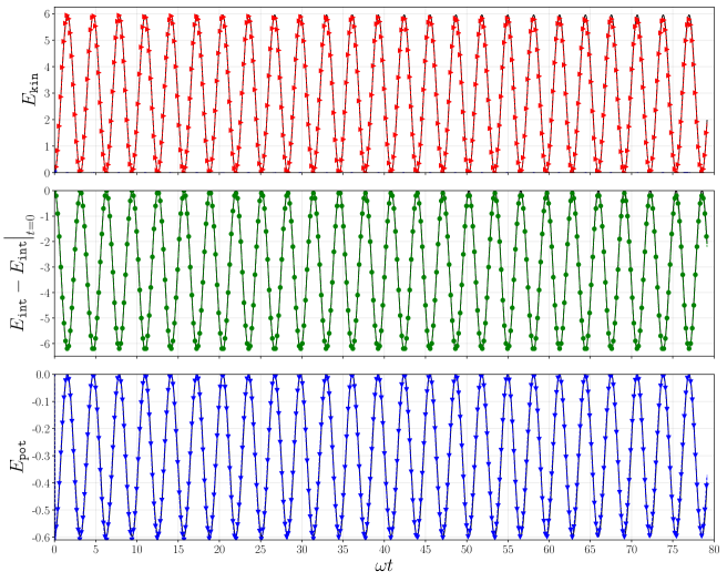
Figure 3: Evolution of the computed kinetic (), internal (), and potential () energies for the Jeans instability using polynomial order $N=3$ on a uniform $16\times 16$ mesh. The analytical () energies are included for reference. Multi-physics coupling is done in every RK stage of the compressible Euler solver with $\mathtt{CFL}_{\mathrm{Eu}}=0.5$ and $\mathtt{CFL}_{\mathrm{Gr}}=0.8$ using CK45.

The Jeans instability problem offers an interesting middle ground to investigate computational efficiency and solution accuracy. This is because the Jeans instability is a more physically relevant test setup than the manufactured solution from Section 3.1.3, but still possesses analytical energy profiles that we can compare against. As such, we run another simulation that employs the alternative gravity coupling procedure of “freezing” the gravitational potential within each RK time step and evolving the hydrodynamic quantities. We demonstrated in Section 3.1.3 that this introduces a first-order temporal error into the approximation; however, it is interesting to examine how such coupling influences the solution quality for the Jeans instability test case.

As such, we again run the multi-physics solver using CK45 time integration for the compressible Euler and hyperbolic gravity solvers with $\mathtt{CFL}_{\mathrm{Eu}}=0.5$ and $\mathtt{CFL}_{\mathrm{Gr}}=0.8$ for time step selection. This time, however, we update the gravitational potential and its gradients after every RK time step of the Euler solver. We present the evolution of the kinetic, internal and potential energy profiles in Fig. 4 as functions of $\omega t$. We, again, see that the dispersion errors are very small for the DG approximation of the Jeans instability with this alternative coupling. But, as time progresses, there is a noticeable loss in amplitude of the different energies due to the first-order errors introduced into the approximation. Such errors can be removed by taking a very small value of $\mathtt{CFL}_{\mathrm{Eu}}$ [72] (for example selecting $\mathtt{CFL}_{\mathrm{Eu}}=0.01$ produces results nearly identical to Fig. 3), effectively reducing the temporal errors to be of lower magnitude to reveal dominate spatial behavior. However, such a small value of $\mathtt{CFL}_{\mathrm{Eu}}$ is computationally prohibitive and further reinforces our finding from Section 3.1.3 that a multi-physics coupling procedure that preserves the underlying order of the spatial approximation is also desirable for practical simulations.

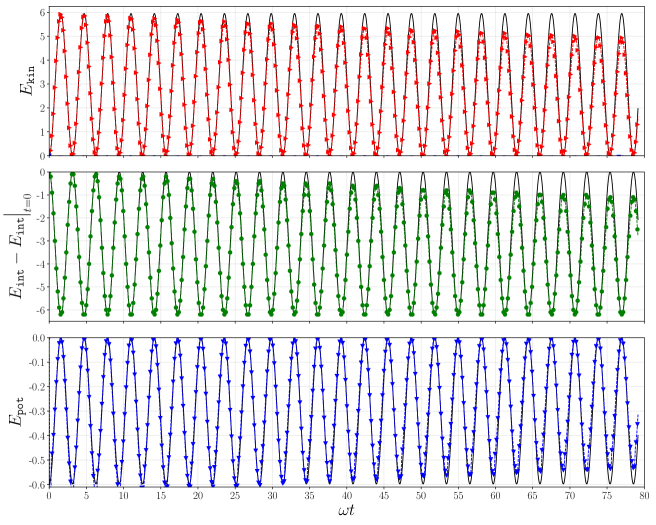
Figure 4: Evolution of the kinetic (), internal (), and potential () energies for the Jeans instability using polynomial order $N=3$ on a uniform $16\times 16$ mesh. The analytical () energies are included for reference. Multi-physics coupling is done in every RK time step of the compressible Euler solver with $\mathtt{CFL}_{\mathrm{Eu}}=0.5$ and $\mathtt{CFL}_{\mathrm{Gr}}=0.8$ using CK45. There is a loss in energy amplitudes due to the first-order coupling.

We also investigate the effect that the optimized method RK3S* from Section 2.3 has in reducing the computational effort for the hyperbolic gravity solver. lne:grav_cycle_start To do so, we introduce a shorthand cost measurement deemed a gravity sub-cycle. This cost measure corresponds to the assembly and evolution of the hyperbolic gravity system by one complete time step in pseudotime within the gravity update loop (see Fig. 2). We note that each gravity sub-cycle consists of five RK stages for either the CK45 or RK3S* time integration schemes. Recall, in each RK stage of the compressible Euler simulation the hyperbolic gravity solver must evolve in pseudotime until the steady-state tolerance of $\mathtt{tol}=10^{-4}$ is reached. lne:pseudotime_4 Thus, an obvious first attempt to improve the computational efficiency of the multi-physics implementation is to reduce the number of gravity lne:grav_cycle_end sub-cycles. We again simulate the Jeans instability with $\mathtt{CFL}_{\mathrm{Eu}}=0.5$ but compare the sub-cycle counts for the hyperbolic gravity solver with the CK45 scheme with $\mathtt{CFL}_{\mathrm{Gr}}=0.8$ against RK3S* with $\mathtt{CFL}_{\mathrm{Gr}}=1.2$. These CFL values led to the largest stable explicit time steps that still produced meaningful simulation results.

Histograms in Fig. 5 visualize the sub-cycle frequency of the hyperbolic gravity solver for these two time integration techniques. Note we have removed outlier gravity sub-cycle values that occur only once (e.g., for the initial solve in the first time step) to better illustrate the trend and overall effort of the hyperbolic gravity solver runs.

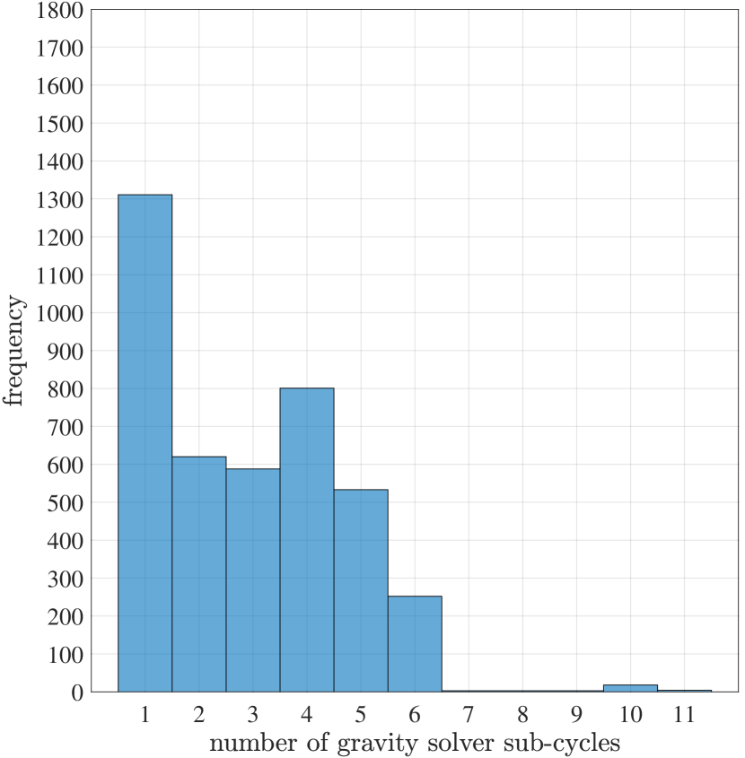
(a) CK45, $\mathtt{CFL}_{\mathrm{Eu}}=0.5$, $\mathtt{CFL}_{\mathrm{Gr}}=0.8$

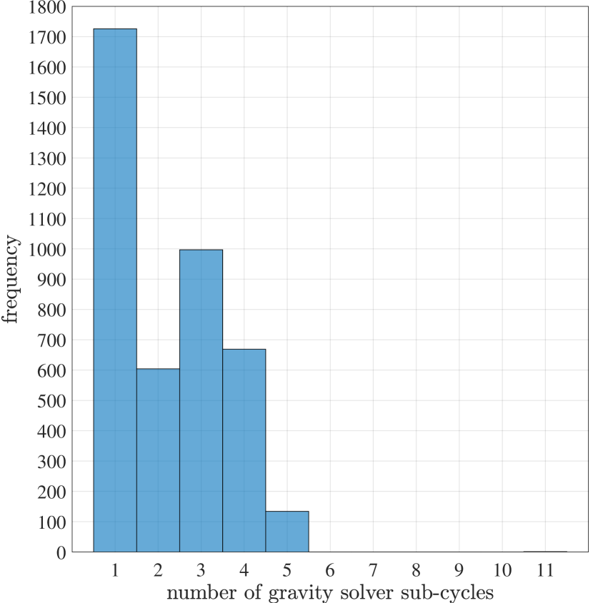
(b) RK3S*, $\mathtt{CFL}_{\mathrm{Eu}}=0.5$, $\mathtt{CFL}_{\mathrm{Gr}}=1.2$

Figure 5: Two runs of the Jeans instability test case with polynomial order $N=3$ on a uniform $16\times 16$ mesh with different explicit time integration methods. Histograms present the frequency of different gravity sub-cycles counts needed for the hyperbolic gravity solver to reach the steady-state tolerance $\mathtt{tol}=10^{-4}$ in each RK stage. Comparison can be made between the number and distribution of gravity solver sub-cycles necessary for CK45 (left) or RK3S* (right) optimized for the hyperbolic diffusion system (2.3).

The results shown in Fig. 5 demonstrate that the number of gravity solver sub-cycles is concentrated near one or two iterations for either time integration scheme. So, using the hyperbolic gravity variables from the previous compressible Euler RK stage as the initial guess for the next hyperbolic gravity solve works well to keep the number sub-cycles to update the gravitational potential small. However, the spread of the sub-cycle iteration number is wider for the standard CK45 time integrator compared to RK3S* that was optimized to take larger explicit time steps for the hyperbolic gravity problem. Apart from the concentration of the sub-cycle distribution it is also noteworthy that the raw number of hyperbolic gravity sub-cycles for CK45 was 12,055 whereas RK3S* required only 9,344. Therefore, not only is the distribution of gravity sub-cycles more skewed toward lower values for RK3S*, but the computational effort for the gravity solver is also decreased by approximately $22\text{\,}\mathrm{\char 37\relax}$. We would like to emphasize that this performance improvement does not negatively impact solution accuracy, as discussed in Section 3.1.3, and that it can be applied immediately if 3S* RK schemes are already supported by the implementation.

3.2.2 Sedov explosion with self-gravity

As a final numerical example we consider a modification of the Sedov blast wave problem that incorporates the effects of gravitational acceleration [68]. The hydrodynamic setup of the Sedov explosion [77] is a difficult one, as it involves strong shocks and complex fluid interactions. We include it to demonstrate the shock capturing and AMR capabilities of Trixi.jl to resolve the cylindrical Sedov blast wave. Additionally, it highlights that the treatment of the gravitational potential as a hyperbolic system (2.3) is immediately amenable to AMR through a standard mortar method. No further considerations are necessary to approximate the gravitational potential on non-conforming meshes.

The initial configuration of the Sedov problem deposits the explosion energy $E$ into a single point in a medium of uniform ambient density $\rho_{\mathrm{am}}$ and pressure $p_{\mathrm{am}}$. In practice, the initialization of the Sedov problem is delicate because this energetic area is typically smaller than the grid resolution. Therefore, we follow an approach similar to Fryxell et al. [2] to convert the explosion energy into a pressure contained within a resolvable area center of radius $r_{\mathrm{ini}}$ by

$$p_{\mathrm{ini}}=\frac{(\gamma-1)E}{\pi r_{\mathrm{ini}}}.$$ (3.17)

This pressure is then used for the discretization points where $r<r_{\mathrm{ini}}$. For the simulation we choose $r_{\mathrm{ini}}$ to be four times as large as the initial grid spacing, which helps to minimize effects due to the Cartesian geometry of the computational grid.

We consider the Sedov explosion parameters in CGS units to be $p_{\mathrm{am}}=10^{-5}$ [dyn cm^-2], $E=1$ [erg], and $v_{1}=v_{2}=0$ [cm s^-1], and we set $\gamma=1.4$. The computational domain $\Omega=[-4,4]^{2}$ [cm²] is discretized by an adaptive mesh with a minimum element length $h=0.03125$ [cm]. Thus, the value $r_{\mathrm{ini}}=0.125$ [cm] is used in (3.17). The gravitational constant is $G=6.674\cdot 10^{-8}$ [cm³g^-1s^-2]. For the gravitational potential it is customary to assume that it vanishes at large distances away from a localized region of non-zero density, e.g., [6, 68, 78]. Therefore, we localize the ambient density, $\rho_{\mathrm{am}}$, to be contained in a disc of radius $r_{\rho}=1$ [cm] such that

$$\rho_{\mathrm{am}}\;[\text{g cm}^{-3}]=\begin{cases}1,&r\leq r_{\rho}\\ 10^{-5},&r>r_{\rho}.\\ \end{cases}$$ (3.18)

The transition between inner and ambient state for both pressure and density is smoothened by a logistic function with steepness $k=150$ [cm^-1]. We set Dirichlet boundary conditions at the four edges of the domain to be the ambient flow states for the hydrodynamic variables and zero for the hyperbolic gravity system.

We approximate the hydrodynamic and hyperbolic gravity solutions with polynomial order $N=3$ and run the simulation to a final time of $T=1.0$. We select a time step with $\mathtt{CFL}_{\mathrm{Eu}}=0.5$ for CK45 and $\mathtt{CFL}_{\mathrm{Gr}}=1.2$ using RK3S*. The compressible Euler solver uses the split-form DGSEM feature of Trixi.jl with the shock capturing scheme by Hennemann et al. [52] as described in Section 2.2, while the hyperbolic gravity solver uses the standard DGSEM formulation. During the simulation, the mesh is adaptively coarsened and refined after every time step of the compressible Euler solver. The mesh resolution spans seven refinement levels, where $h=2.0$ [cm] at the base level ($l=2$) and $h=0.03125$ [cm] at the highest refinement level ($l=8$), see Fig. 6. We evaluate the same indicator function for AMR as for shock capturing. Elements with $\alpha_{\text{AMR}}>0.0003$ are assigned a target refinement level of $l=8$, all other elements are assigned a target level of $l=2$. The value of the AMR indicator $\lambda$ is based on whether an element matches its target level or needs to be adapted, and the 2:1 balancing algorithm automatically ensures a smoothly varying mesh resolution. For details, see the description in A.

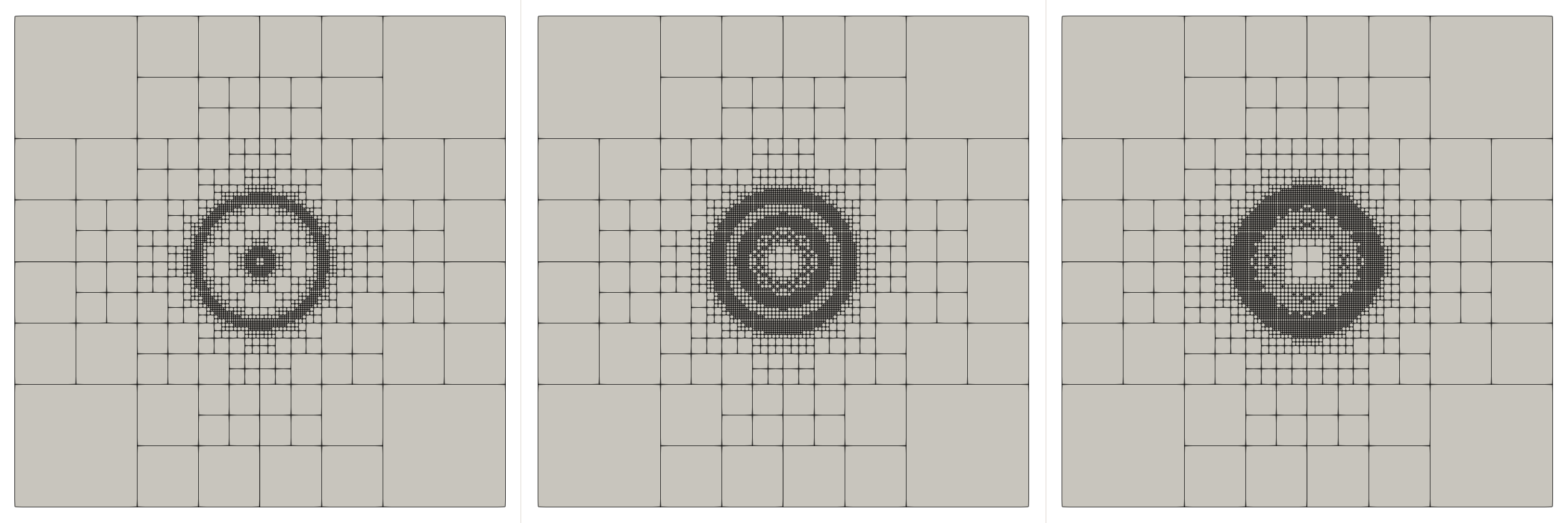
Figure 6: Adaptive mesh for self-gravitating Sedov explosion with seven different refinement levels at $T=0.0$ (left), $T=0.5$ (center), and $T=1.0$ (right).

We present the approximate density and gravitational potential at the intermediate time $T=0.5$ and final time $T=1.0$ in the first and third rows of Fig. 7. The density pseudocolor plots, in the top row, also give an overlay of the joint AMR grid that is shared by both solvers. The second and fourth rows of Fig. 7 extract a slice of the density and gravitational potential solutions along the horizontal line from the origin to the edge of the domain in the positive $x$-direction. The shapes of these one-dimensional profiles match well with the results for a similar self-gravitating Sedov explosion test available in [68]. Furthermore, we create a reference solution for this test problem using a high-resolution run on a uniform mesh at the finest AMR level with polynomial order $N=3$ in each spatial direction. The one-dimensional profile slices in Fig. 7 reveal that the solutions on the adaptive mesh are virtually indistinguishable from the reference result.

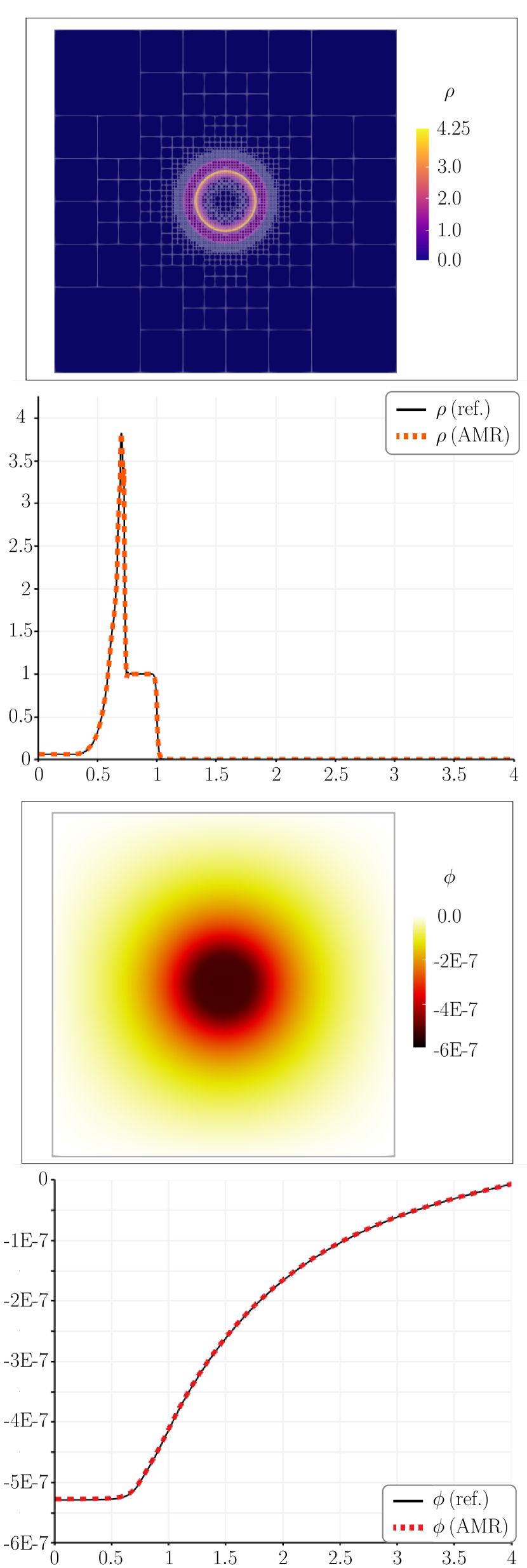
(a) $T=0.5$

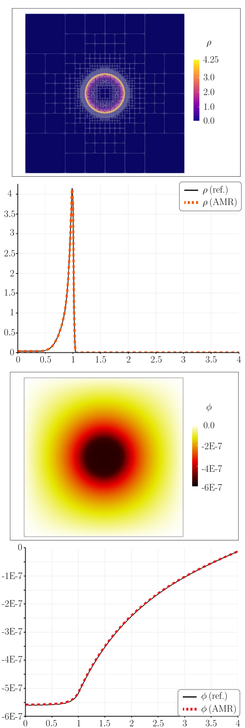
(b) $T=1.0$

Figure 7: Self-gravitating Sedov explosion approximated with polynomial order $N=3$ on an AMR grid with four levels of possible refinement. (first and third row) Two dimensional plots of the density and gravitational potential at two times. The white overlay of squares in the density plots shows the AMR grids used by both solvers. (second and last row) One dimensional slices of the solutions along a line from the origin to the edge of the domain in the positive $x$-direction.

As a final result, the computational effort of Trixi.jl to solve the self-gravitating Sedov explosion with a uniform and an adaptive mesh is presented in Table 7. It is worth noting that the percentage figures of the gravity solver are comparable to other multi-physics solvers. lne:grav_percent_again_startFor instance, the percentage of the total runtime spent in the gravity solver was reported for other astrophysical simulation frameworks to be approximately 88–92% in [79, Table 1], 43–78% in [80, Fig. 2], 25–36% in [81, Fig. C1], 85% in [30, Fig. 6], 34–72% in [15, Table 5], or 14–50% in [82, Fig. 6]. This underpins that the presented hyperbolic formulation of the gravity equation offers an alternative solution strategy to existing gravity solvers. lne:grav_percent_again_end We further see that activating AMR for this test case decreases the overall run time by approximately a factor of 19, while there is minimal difference between the reference and adaptive solutions for the self-gravitating Sedov blast wave. This demonstrates a novel advantage of non-conforming DG with AMR capabilities and the hyperbolic gravity formulation. It is possible to accurately and rapidly approximate the solution of an elliptic problem in a hyperbolic fashion.

Table 7: Run time measurements for simulating the self-gravitating Sedov blast with a uniform and an adaptive mesh. The uniform mesh is at refinement level $l=8$, while the adaptive mesh is at multiple levels $l\in[2,8]$ with adaptation performed after every time step of the compressible Euler solver.

	Uniform mesh		Adaptive mesh
Compressible Euler solver	$652.8\,\textrm{s}$	$46.3\%$	$39.2\,\textrm{s}$	$52.4\%$
Gravity solver	$758.0\,\textrm{s}$	$53.7\%$	$26.5\,\textrm{s}$	$35.4\%$
AMR	–	–	$9.1\,\textrm{s}$	$12.1\%$
Total	$1410.8\,\textrm{s}$	$100.0\%$	$74.8\,\textrm{s}$	$100.0\%$

4 Conclusions

In this paper, we adapted Nishikawa’s idea for solving the Poisson equation as a hyperbolic diffusion system in the context of self-gravitating flows. lne:concl_motive_1_start In doing so, we converted the equation for a Newtonian gravitational potential into a system of hyperbolic gravity equations. lne:concl_motive_1_end

Then, the hydrodynamics and hyperbolic gravity approximations were both built from a nodal discontinuous Galerkin method. This allowed us to treat the elliptic problem for Newtonian gravity in a fully explicit hyperbolic fashion, and we verified that we are able to obtain high-order accurate solutions for both single- and multi-physics simulations. By treating the elliptic gravity problem in a purely hyperbolic way, its numerical approximation inherits the full functionality and accuracy of the nodal discontinuous Galerkin method. Most notably, the ability to do non-conforming approximations via mortars and to solve the elliptic gravity problem on an adaptive grid is retained without any modifications. In addition, coupling the flow and the gravity solver in each Runge-Kutta stage preserves and carries over the high-order benefits from the single-physics into the multi-physics context. Borrowing ideas from the time integration community, we optimized a Runge-Kutta scheme to reduce computational effort and to accelerate the hyperbolic gravity solution to steady state.

lne:concl_motive_2_start From the numerical results, we found that the fractions of computational effort for the compressible Euler and hyperbolic gravity solvers were comparable to other multi-physics solvers. Thus, for problems in self-gravitating gas dynamics, the use of hyperbolic diffusion methodology provides an interesting alternative to a classical iterative elliptic solver. The further development and optimization of the hyperbolic gravity multi-physics approach is the subject of ongoing research. lne:concl_motive_2_end All results in this paper were obtained with the open-source simulation framework Trixi.jl, which is available as a registered Julia package. To allow reproducing our findings and to invite further collaboration, we also made the corresponding setup files publicly available online [32].

Appendix A Algorithms and implementation

lne:appendix_start In the following, we present in detail the control flow for a single-physics simulation with Trixi.jl. The algorithms to enable coupled multi-physics simulations were already introduced in Section 2.4. Here, the purpose is to illustrate how simple it is to extend an existing single-physics solver for hyperbolic conservation laws to a multi-physics solver for self-gravitating gas dynamics simulations.

A two-dimensional quadtree mesh forms the basis of the simulation framework Trixi.jl, which can be refined adaptively during a simulation to meet dynamically changing resolution requirements. Several systems of equations are supported, including the compressible Euler equations, ideal magnetohydrodynamics equations with divergence cleaning [83], and hyperbolic diffusion equations [16, 24]. They are discretized in space by a high-order DG method and integrated in time by explicit Runge-Kutta schemes, as described in Section 2. Trixi.jl is parallelized with a thread-based shared memory approach and written in Julia [84].

During the initialization phase, the simulation is set up by creating a mesh instance according to the simulation parameters. Next, a solver instance is created that uses the mesh to build up the required data structures for the DG method, and the solution is initialized. To obtain the optimal mesh for the initial solution state, the adaptive mesh refinement algorithm (AMR) is called to adapt the mesh according to the initial conditions, before initializing the solution again on this refined mesh. This process is repeated until the mesh no longer changes or a predetermined number of sub-cycles is reached.

The execution phase begins when entering the main loop, where first the current stable time step is determined from the CFL condition. Next, the time integration loop is entered, where the solver is used to compute the spatial derivative once for each explicit Runge-Kutta stage. After the solution has been advanced to the new time step, the AMR algorithm is called to adapt the mesh. The main loop will then continue until either the desired simulation time is reached (flow-type simulations) or the residual falls below a specified threshold that defines “steady state” (hyperbolic diffusion-type simulations).

To adaptively refine the mesh, the adaptation algorithm first queries the DG solver for a refinement indicator value $\lambda\in\{-1,0,1\}$ for each DG element. The specific procedure to calculate $\lambda$ is problem dependent (one example is given in Section 3.2.2). An indicator value greater than zero indicates that an element (and its corresponding grid cell) should be refined and a value less than zero indicates that an element should be coarsened. A zero value means that the element should remain unchanged. Next, the mesh and the solver are jointly adapted: In the first step, all cells with an indicator value of $\lambda=1$ are refined. A smoothing algorithm ensures that the quadtree remains balanced, i.e., additional cells might be refined to retain a 2:1 relationship between neighboring cells. The corresponding DG elements are then refined as well, using polynomial interpolation to transfer the solution from the original coarse cell to the newly created refined cell. In the second step, the same procedure is repeated to coarsen all cells with an indicator value of $\lambda=-1$. In case of conflicts, refinement overrides coarsening to retain a high solution quality. That is, if a cell originally marked for coarsening has already been refined in the first step to rebalance the quadtree, it will not be coarsened. lne:appendix_end

References

- [1] J. M. Stone, M. L. Norman, ZEUS-2D: A radiation magnetohydrodynamics code for astrophysical flows in two space dimensions. I - The hydrodynamic algorithms and tests. II - The magnetohydrodynamic algorithms and tests, Astrophys. J. Supplement Series 80 (1992) 753. doi:10.1086/191680.
- [2] B. Fryxell, K. Olson, P. Ricker, F. Timmes, M. Zingale, D. Lamb, P. MacNeice, R. Rosner, J. Truran, H. Tufo, FLASH: An adaptive mesh hydrodynamics code for modeling astrophysical thermonuclear flashes, The Astrophysical Journal Supplement Series 131 (1) (2000) 273–334.
- [3] R. Teyssier, Cosmological hydrodynamics with adaptive mesh refinement, Astron. Astrophys. 385 (1) (2002) 337–364. doi:10.1051/0004-6361:20011817.
- [4] A. S. Almgren, V. E. Beckner, J. B. Bell, M. S. Day, L. H. Howell, C. C. Joggerst, M. J. Lijewski, A. Nonaka, M. Singer, M. Zingale, CASTRO: A New Compressible Astrophysical Solver. I. Hydrodynamics and Self-gravity, Astrophys. J. 715 (2) (2010) 1221–1238. doi:10.1088/0004-637x/715/2/1221.
- [5] G. L. Bryan, M. L. Norman, B. W. O’Shea, T. Abel, J. H. Wise, M. J. Turk, D. R. Reynolds, D. C. Collins, P. Wang, S. W. Skillman, B. Smith, R. P. Harkness, J. Bordner, J. hoon Kim, M. Kuhlen, H. Xu, N. Goldbaum, C. Hummels, A. G. Kritsuk, E. Tasker, S. Skory, C. M. Simpson, O. Hahn, J. S. Oishi, G. C. So, F. Zhao, R. Cen, Y. Li, ENZO: An Adaptive Mesh Refinement Code for Astrophysics, Astrophys. J. Supplement Series 211 (2) (2014) 19. doi:10.1088/0067-0049/211/2/19.
- [6] D. A. Hubber, G. P. Rosotti, R. A. Booth, GANDALF–Graphical astrophysics code for -body dynamics and Lagrangian fluids, Monthly Notices of the Royal Astronomical Society 473 (2) (2018) 1603–1632.
- [7] J. M. Stone, K. Tomida, C. J. White, K. G. Felker, The Athena++ Adaptive Mesh Refinement Framework: Design and Magnetohydrodynamic Solvers, Astrophys. J. Supplement Series (2020). arXiv:2005.06651v1, doi:10.3847/1538-4365/ab929b.
- [8] H.-Y. K. Yang, P. M. Ricker, P. M. Sutter, The Influence of Concentration and Dynamical State on Scatter in the Galaxy Cluster Mass-Temperature Relation, Astrophys. J. 699 (1) (2009) 315–329. doi:10.1088/0004-637x/699/1/315.
- [9] J. A. ZuHone, M. Markevitch, R. E. Johnson, Stirring Up the Pot: Can Cooling Flows in Galaxy Clusters be Quenched by Gas Sloshing?, Astrophys. J. 717 (2) (2010) 908–928. doi:10.1088/0004-637x/717/2/908.
- [10] S. M. Couch, C. Graziani, N. Flocke, An Improved Multipole Approximation for Self-gravity and Its Importance for Core-collapse Supernova Simulations, Astrophys. J. 778 (2) (2013) 181. doi:10.1088/0004-637x/778/2/181.
- [11] M. A. Latif, S. Zaroubi, M. Spaans, The impact of Lyman trapping on the formation of primordial objects, Mon. Not. R. Astron. Soc. 411 (3) (2010) 1659–1670. doi:10.1111/j.1365-2966.2010.17796.x.
- [12] C. Federrath, R. S. Klessen, The Star Formation Rate of Turbulent Magnetized Clouds: Comparing Theory, Simulations, and Observations, Astrophys. J. 761 (2) (2012) 156. doi:10.1088/0004-637x/761/2/156.
- [13] P. M. Ricker, A Direct Multigrid Poisson Solver for Oct-Tree Adaptive Meshes, Astrophys. J. Supplement Series 176 (1) (2008) 293–300. doi:10.1086/526425.
- [14] J. Barnes, P. Hut, A hierarchical O(N log N) force-calculation algorithm, Nat. 324 (6096) (1986) 446–449. doi:10.1038/324446a0.
- [15] R. Wünsch, S. Walch, F. Dinnbier, A. Whitworth, Tree-based solvers for adaptive mesh refinement code FLASH – I: gravity and optical depths, Mon. Not. R. Astron. Soc. 475 (3) (2018) 3393–3418. doi:10.1093/mnras/sty015.
- [16] H. Nishikawa, A first-order system approach for diffusion equation. I: Second-order residual-distribution schemes, J. Comput. Phys. 227 (1) (2007) 315–352. doi:10.1016/j.jcp.2007.07.029.
- [17] C. Cattaneo, A form of heat-conduction equations which eliminates the paradox of instantaneous propagation, Ct. R. Acad. Sci., Paris 247 (1958) 431–433.
- [18] G. B. Nagy, O. E. Ortiz, O. A. Reula, The behavior of hyperbolic heat equations’ solutions near their parabolic limits, J. Math. Phys. 35 (8) (1994) 4334–4356. doi:10.1063/1.530856.
- [19] R. J. Leveque, H. C. Yee, A study of numerical methods for hyperbolic conservation laws with stiff source terms, J. Comput. Phys. 86 (1) (1990) 187–210. doi:10.1016/0021-9991(90)90097-k.
- [20] L. Li, J. Lou, H. Luo, H. Nishikawa, A new formulation of hyperbolic Navier-Stokes solver based on finite volume method on arbitrary grids, in: 2018 Fluid Dynamics Conference, 2018, p. 4160.
- [21] H. Nishikawa, First, second, and third order finite-volume schemes for advection–diffusion, J. Comput. Phys. 273 (2014) 287–309. doi:10.1016/j.jcp.2014.05.021.
- [22] H. T. Ahn, Hyperbolic cell-centered finite volume method for steady incompressible Navier-Stokes equations on unstructured grids, Computers & Fluids 200 (2020) 104434.
- [23] A. S. Chamarthi, K. Komurasaki, R. Kawashima, High-order upwind and non-oscillatory approach for steady state diffusion, advection–diffusion and application to magnetized electrons, Journal of Computational Physics 374 (2018) 1120–1151.
- [24] J. Lou, X. Liu, H. Luo, H. Nishikawa, Reconstructed discontinuous Galerkin methods for hyperbolic diffusion equations on unstructured grids, Communications in Computational Physics 25 (2019) 1302–1327.
- [25] A. Mazaheri, H. Nishikawa, Efficient high-order discontinuous Galerkin schemes with first-order hyperbolic advection–diffusion system approach, Journal of Computational Physics 321 (2016) 729–754.
- [26] D. C. Black, P. Bodenheimer, Evolution of rotating interstellar clouds. I - Numerical techniques, Astrophys. J. 199 (1975) 619. doi:10.1086/153729.
- [27] D. W. Peaceman, H. H. Rachford, The Numerical Solution of Parabolic and Elliptic Differential Equations, J. Soc. Ind. Appl. Math. 3 (1) (1955) 28–41. doi:10.1137/0103003.
- [28] J. Krebs, W. Hillebrandt, The interaction of supernova shockfronts and nearby interstellar clouds, Astron. Astrophys. 128 (2) (1983) 411–419.
- [29] M. L. Norman, K.-H. A. Winkler, 2-D Eulerian Hydrodynamics with Fluid Interfaces, Self-Gravity and Rotation, in: Astrophysical Radiation Hydrodynamics, 1986, pp. 187–222.
- [30] R. Hirai, H. Nagakura, H. Okawa, K. Fujisawa, Hyperbolic self-gravity solver for large scale hydrodynamical simulations, Phys. Rev. D 93 (8) (2016). doi:10.1103/physrevd.93.083006.
-
[31]
M. Schlottke-Lakemper, G. J. Gassner, H. Ranocha, A. R. Winters,
Trixi.jl: A tree-based
numerical simulation framework for hyperbolic PDEs written in Julia (2020).
doi:10.5281/zenodo.3996439.
URL https://github.com/trixi-framework/Trixi.jl -
[32]
M. Schlottke-Lakemper, A. R. Winters, H. Ranocha, G. J. Gassner,
Self-gravitating
gas dynamics simulations with Trixi.jl (2020).
doi:10.5281/zenodo.3996575.
URL https://github.com/trixi-framework/paper-self-gravitating-gas-dynamics - [33] S. Chandrasekhar, Hydrodynamic and Hydromagnetic Stability, Dover Books on Physics Series, Dover Publications, 1961.
- [34] H. Nishikawa, First-, second-, and third-order finite-volume schemes for diffusion, J. Comput. Phys. 256 (2014) 791–805. doi:10.1016/j.jcp.2013.09.024.
- [35] H. Nishikawa, Y. Nakashima, Dimensional scaling and numerical similarity in hyperbolic method for diffusion, J. Comput. Phys. 355 (2018) 121–143.
- [36] H. Gomez, I. Colominas, F. Navarrina, J. París, M. Casteleiro, A hyperbolic theory for advection-diffusion problems: Mathematical foundations and numerical modeling, Archives of Computational Methods in Engineering 17 (2) (2010) 191–211.
- [37] D. A. Kopriva, Implementing Spectral Methods for Partial Differential Equations: Algorithms for Scientists and Engineers, Springer, 2009. doi:10.1007/978-90-481-2261-5.
- [38] F. Hindenlang, G. J. Gassner, C. Altmann, A. Beck, M. Staudenmaier, C.-D. Munz, Explicit discontinuous Galerkin methods for unsteady problems, Comput. Fluids 61 (2012) 86–93. doi:10.1016/j.compfluid.2012.03.006.
- [39] M. Schlottke-Lakemper, A. Niemöller, M. Meinke, W. Schröder, Efficient parallelization for volume-coupled multiphysics simulations on hierarchical Cartesian grids, Comput. Methods Appl. Mech. Eng. 352 (2019) 461–487. doi:10.1016/j.cma.2019.04.032.
- [40] A. Harten, P. D. Lax, B. v. Leer, On upstream differencing and Godunov-type schemes for hyperbolic conservation laws, SIAM review 25 (1) (1983) 35–61.
- [41] Eleuterio F. Toro, Riemann Solvers and Numerical Methods for Fluid Dynamics, Springer-Verlag Berlin Heidelberg, 2009.
- [42] G. J. Gassner, A Skew-Symmetric Discontinuous Galerkin Spectral Element Discretization and Its Relation to SBP-SAT Finite Difference Methods, SIAM J. Sci. Comput. 35 (3) (2013) A1233–A1253. doi:10.1137/120890144.
- [43] T. C. Fisher, M. H. Carpenter, J. Nordström, N. K. Yamaleev, C. Swanson, Discretely conservative finite-difference formulations for nonlinear conservation laws in split form: Theory and boundary conditions, J. Comput. Phys. 234 (2013) 353–375. doi:10.1016/j.jcp.2012.09.026.
- [44] M. H. Carpenter, T. C. Fisher, E. J. Nielsen, S. H. Frankel, Entropy Stable Spectral Collocation Schemes for the Navier–Stokes Equations: Discontinuous Interfaces, SIAM J. Sci. Comput. 36 (5) (2014) B835–B867. doi:10.1137/130932193.
- [45] G. J. Gassner, A. R. Winters, D. A. Kopriva, Split form nodal discontinuous Galerkin schemes with summation-by-parts property for the compressible Euler equations, J. Comput. Phys. 327 (2016) 39–66. doi:10.1016/j.jcp.2016.09.013.
- [46] G. J. Gassner, A. R. Winters, F. J. Hindenlang, D. A. Kopriva, The BR1 Scheme is Stable for the Compressible Navier–Stokes Equations, J. Sci. Comput. 77 (1) (2018) 154–200. doi:10.1007/s10915-018-0702-1.
- [47] E. Tadmor, Entropy stability theory for difference approximations of nonlinear conservation laws and related time-dependent problems, Acta Numerica 12 (2003) 451–512. doi:10.1017/S0962492902000156.
- [48] F. Ismail, P. L. Roe, Affordable, entropy-consistent Euler flux functions II: Entropy production at shocks, Journal of Computational Physics 228 (15) (2009) 5410–5436. doi:10.1016/j.jcp.2009.04.021.
- [49] P. Chandrashekar, Kinetic energy preserving and entropy stable finite volume schemes for compressible Euler and Navier-Stokes equations, Communications in Computational Physics 14 (5) (2013) 1252–1286. doi:10.4208/cicp.170712.010313a.
- [50] H. Ranocha, Generalised summation-by-parts operators and entropy stability of numerical methods for hyperbolic balance laws, Ph.D. thesis, TU Braunschweig (02 2018).
- [51] P. Chandrashekar, Kinetic energy preserving and entropy stable finite volume schemes for compressible Euler and Navier-Stokes equations, Communications in Computational Physics 14 (2013) 1252–1286.
- [52] S. Hennemann, A. M. Rueda-Ramírez, F. J. Hindenlang, G. J. Gassner, A provably entropy stable subcell shock capturing approach for high order split form DG for the compressible Euler equations, J. Comput. Phys. 426 (2021) 109935. doi:https://doi.org/10.1016/j.jcp.2020.109935.
- [53] D. A. Kopriva, A Conservative Staggered-Grid Chebyshev Multidomain Method for Compressible Flows. II. A Semi-Structured Method, J. Comput. Phys. 128 (2) (1996) 475–488. doi:10.1006/jcph.1996.0225.
- [54] D. A. Kopriva, S. L. Woodruff, M. Hussaini, Computation of electromagnetic scattering with a non-conforming discontinuous spectral element method, Int. J. Numer. Methods Eng. 53 (2002) 105–222. doi:10.1002/nme.394.
- [55] T. Bui-Thanh, O. Ghattas, Analysis of an -nonconforming discontinuous Galerkin spectral element method for wave propagation, SIAM Journal on Numerical Analysis 50 (3) (2012) 1801–1826.
- [56] M. H. Carpenter, C. Kennedy, Fourth-order 2N-storage Runge-Kutta schemes, NASA Report TM 109112, NASA Langley Research Center (1994).
- [57] N. A. Loppi, F. D. Witherden, A. Jameson, P. E. Vincent, Locally adaptive pseudo-time stepping for high-order flux reconstruction, Journal of Computational Physics 399 (2019) 108913. doi:10.1016/j.jcp.2019.108913.
- [58] H. Ranocha, L. Dalcin, M. Parsani, D. I. Ketcheson, Optimized Runge-Kutta methods with automatic step size control for compressible computational fluid dynamics (04 2021). arXiv:2104.06836.
- [59] B. C. Vermeire, N. A. Loppi, P. E. Vincent, Optimal embedded pair Runge-Kutta schemes for pseudo-time stepping, Journal of Computational Physics (2020) 109499doi:10.1016/j.jcp.2020.109499.
- [60] M. Parsani, D. I. Ketcheson, W. Deconinck, Optimized explicit Runge-Kutta schemes for the spectral difference method applied to wave propagation problems, SIAM Journal on Scientific Computing 35 (2) (2013) A957–A986. doi:10.1137/120885899.
- [61] D. Ketcheson, A. Ahmadia, Optimal stability polynomials for numerical integration of initial value problems, Communications in Applied Mathematics and Computational Science 7 (2) (2013) 247–271. doi:10.2140/camcos.2012.7.247.
- [62] D. I. Ketcheson, Runge-Kutta methods with minimum storage implementations, Journal of Computational Physics 229 (5) (2010) 1763–1773. doi:10.1016/j.jcp.2009.11.006.
-
[63]
D. I. Ketcheson, M. Parsani, Z. J. Grant, A. Ahmadia, H. Ranocha,
RK-Opt: A package for the design
of numerical ODE solvers, Journal of Open Source Software 5 (54) (2020)
2514.
doi:10.21105/joss.02514.
URL https://github.com/ketch/RK-Opt -
[64]
MathWorks, MATLAB (2019).
URL https:/mathworks.com/products/matlab.html -
[65]
D. I. Ketcheson, H. Ranocha, M. Parsani, U. bin Waheed, Y. Hadjimichael,
NodePy: A package for the analysis
of numerical ODE solvers, Journal of Open Source Software 5 (55) (2020)
2515.
doi:10.21105/joss.02515.
URL https://github.com/ketch/nodepy - [66] G. Gassner, F. Hindenlang, C. Munz, A Runge-Kutta based discontinuous Galerkin method with time accurate local time stepping, Adaptive High-Order Methods in Computational Fluid Dynamics 2 (2011) 95–118.
- [67] J. H. Jeans, The stability of a spherical nebula, Philosophical Transactions of the Royal Society of London A: Mathematical, Physical and Engineering Sciences 199 (312-320) (1902) 1–53. doi:10.1098/rsta.1902.0012.
-
[68]
Flash Center for Computational Science, University of Chicago,
FLASH
User’s Guide.
URL http://flash.uchicago.edu/site/flashcode/user_support/flash4_ug_4p62.pdf - [69] P. Ricker, A direct multigrid Poisson solver for oct-tree adaptive meshes, The Astrophysical Journal Supplement Series 176 (1) (2008) 293.
- [70] J. Huang, L. Greengard, A fast direct solver for elliptic partial differential equations on adaptively refined meshes, SIAM Journal on Scientific Computing 21 (4) (1999) 1551–1566.
- [71] J. Markert, private communication (April 2021).
- [72] D. Derigs, A. R. Winters, G. J. Gassner, S. Walch, A novel high-order, entropy stable, 3D AMR MHD solver with guaranteed positive pressure, Journal of Computational Physics 317 (2016) 223–256.
- [73] D. Hubber, S. Goodwin, A. P. Whitworth, Resolution requirements for simulating gravitational fragmentation using SPH, Astronomy & Astrophysics 450 (3) (2006) 881–886.
-
[74]
J. Binney, S. Tremaine,
Galactic Dynamics:
Second Edition, Princeton Series in Astrophysics, Princeton University
Press, 2011.
URL https://books.google.se/books?id=6mF4CKxlbLsC - [75] W. Bonnor, Jeans’ formula for gravitational instability, Monthly Notices of the Royal Astronomical Society 117 (1) (1957) 104–117.
- [76] M. Ainsworth, Dispersive and dissipative behaviour of high order discontinuous Galerkin finite element methods, Journal of Computational Physics 198 (2004) 106–130.
- [77] L. I. Sedov, Similarity and dimensional methods in mechanics, CRC press, 1993.
- [78] M. P. Katz, M. Zingale, A. C. Calder, F. D. Swesty, A. S. Almgren, W. Zhang, White dwarf mergers on adaptive meshes. I. methodology and code verification, The Astrophysical Journal 819 (2) (2016) 94.
- [79] V. Springel, N. Yoshida, S. D. White, GADGET: a code for collisionless and gasdynamical cosmological simulations, New Astron. 6 (2) (2001) 79–117. doi:https://doi.org/10.1016/S1384-1076(01)00042-2.
- [80] A. S. Almgren, V. E. Beckner, J. B. Bell, M. S. Day, L. H. Howell, C. C. Joggerst, M. J. Lijewski, A. Nonaka, M. Singer, M. Zingale, CASTRO: A new compressible astrophysical solver. I. Hydrodynamics and self-gravity, Astrophys. J. 715 (2) (2010) 1221–1238. doi:10.1088/0004-637x/715/2/1221.
- [81] M. Vogelsberger, D. Sijacki, D. Kereš, V. Springel, L. Hernquist, Moving mesh cosmology: numerical techniques and global statistics, Mon. Not. R. Astron. Soc. 425 (4) (2012) 3024–3057. doi:10.1111/j.1365-2966.2012.21590.x.
- [82] S. Moon, W.-T. Kim, E. C. Ostriker, A Fast Poisson Solver of Second-order Accuracy for Isolated Systems in Three-dimensional Cartesian and Cylindrical Coordinates, Astrophys. J. Supplement Series 241 (2) (2019) 24. doi:10.3847/1538-4365/ab09e9.
- [83] D. Derigs, A. R. Winters, G. J. Gassner, S. Walch, M. Bohm, Ideal GLM-MHD: About the entropy consistent nine-wave magnetic field divergence diminishing ideal magnetohydrodynamics equations, Journal of Computational Physics 364 (2018) 420–467.
- [84] J. Bezanson, A. Edelman, S. Karpinski, V. B. Shah, Julia: A fresh approach to numerical computing, SIAM Review 59 (1) (2017) 65–98. arXiv:1411.1607, doi:10.1137/141000671.