Supplementary_material

Unpolarized and helicity generalized parton distributions
of the proton within lattice QCD

Abstract

We present the first calculation of the $x$-dependence of the proton generalized parton distributions (GPDs) within lattice QCD. Results are obtained for the isovector unpolarized and helicity GPDs. We compute the appropriate matrix elements of fast-moving protons coupled to non-local operators containing a Wilson line. We present results for proton momenta $0.83,\,1.25,\,1.67$ GeV, and momentum transfer squared $0.69,\,1.38$ GeV². These combinations include cases with zero and nonzero skewness. The calculation is performed using one ensemble of two degenerate mass light, a strange and a charm quark of maximally twisted mass fermions with a clover term. The lattice results are matched to the light-cone GPDs using one-loop perturbation theory within the framework of large momentum effective theory. The final GPDs are given in the ${\overline{\rm MS}}$ scheme at a scale of 2 GeV.

Introduction. Quantum Chromodynamics (QCD) is the fundamental theory describing the strong interactions among quarks and gluons (partons). The strong force is responsible for binding partons into hadrons, such as the proton, that makes the bulk of the visible matter in the universe. Studying how the properties of protons emerge from the underlying constituents and their interactions has been an important experimental and theoretical endeavor since the mid-20^th century. These studies led to the realization that high-energy scattering processes can be factorized into perturbative and non-perturbative parts. The latter includes information about the parton structure of the proton Collins et al. (1989). This resulted in the introduction of a complete set of key quantities, namely the parton distribution functions (PDFs) Collins et al. (1989), generalized parton distributions (GPDs) Ji (1997a); Radyushkin (1996); Mueller et al. (1994), and transverse momentum dependent distributions (TMDs) Collins (2003); Ji et al. (2005). These describe the non-perturbative dynamics of the proton, and in general hadrons, in terms of their constituent quarks and gluons Collins and Soper (1982).

There are two unpolarized GPDs, $H^{q}(x,\xi,t)$ and $E^{q}(x,\xi,t)$, and two helicity GPDs, $\widetilde{H}^{q}(x,\xi,t)$ and $\widetilde{E}^{q}(x,\xi,t)$. The superscript $q$ refers to a given quark flavor, and here we study the isovector combination $u-d$. GPDs are functions not only of the longitudinal momentum fraction $x$ ($0\leq x\leq 1$) carried by the partons, but also of the skewness $\xi\equiv-\Delta^{+}/2P^{+}$ and the momentum transfer squared, $t\equiv\Delta^{2}$. $\Delta^{+}$ and $P^{+}$ are the plus component of the momentum transfer and the average proton momentum, respectively. Two kinematical regions arise based on the values of $\xi$ and $x$: the so-called Dokshitzer-Gribov-Lipatov-Altarelli-Parisi (DGLAP) region Dokshitzer (1977); Gribov and Lipatov (1972); Lipatov (1975); Altarelli and Parisi (1977) defined for $x>|\xi|$, and the Efremov-Radyushkin-Brodsky-Lepage (ERBL) Efremov and Radyushkin (1980); Lepage and Brodsky (1980) region for $x<|\xi|$. Physical content can be attributed to each region Ji (1998) using light-cone coordinates and the light-cone gauge. In the positive- (negative-) $x$ DGLAP region, the GPDs correspond to the amplitude of removing a quark (antiquark) of momentum $k$ from the hadron, and then inserting it back with momentum $k+\Delta$. In the ERBL region, the GPD is the amplitude for removing a quark-antiquark pair with momentum $-\Delta$.

While GPDs are multidimensional objects, they lead to simpler quantities when certain limits are taken, or when integrating over selected variables. For example, the forward limit of the unpolarized case, $\Delta=0$, gives the quark, $f_{1}(x)=H^{q}(x,0,0)$, and antiquark PDFs, $\overline{f}_{1}(x)=-H^{q}(-x,0,0)$. Equivalently, in the helicity case one has $g_{1}(x)=\widetilde{H}^{q}(x,0,0)$ and $\overline{g}_{1}(x)=\widetilde{H}^{q}(-x,0,0)$. Integrating over $x$ for nonzero $\Delta$, GPDs give the usual FFs. Taking integrals of GPDs over $x$ leads to a tower of Mellin moments that also have a physical interpretation. such as the total angular momentum of quarks using Ji’s sum rule Ji (1997a).

The connection of GPDs with other quantities demonstrates the information they encode, in both coordinate and momentum spaces. GPDs are accessed through deeply virtual Compton scattering (DVCS) and deeply virtual meson production (DVMP) Ji (1997b). Despite their importance, it is very difficult to extract them experimentally, even though data are available since the early 2000’s. These data are limited, covering a small kinematic region, and are indirectly related to GPDs through the Compton FFs. This poses limitations in their extraction, and the fact that more than one independent measurements are needed to disentangle them Diehl (2003); Ji (2004); Belitsky and Radyushkin (2005); Kumericki et al. (2016).

Nevertheless, the interest in GPDs is renewed due to the advances both on the experimental and the theoretical side, as well as the expertise gained from recent studies of PDFs. It is, thus, of utmost importance to have ab initio computations of GPDs, that will help map them over different regions of $x$, $\xi$, and $t$. Lattice QCD is the only known formulation that allows a quantitative study of QCD directly using its Lagrangian. Lattice QCD is based on a discretization of Euclidean spacetime and relies on large-scale simulations.

Since parton distributions are light-cone correlation functions Collins (2011), it is not straightforward to calculate them using the Euclidean lattice formulation of QCD. The large momentum effective theory (LaMET) proposed by Ji Ji (2013) provides a promising theoretical framework to extract light-cone quantities using matrix elements computed in lattice QCD. Within LaMET Ji (2014); Xiong et al. (2014), one can access light-cone quantities via matrix elements of boosted hadrons coupled with non-local spatial operators, which are calculable on the lattice, and yield what is referred to as quasi-distributions. The first investigations led to encouraging results on the determination of PDFs Lin et al. (2015); Alexandrou et al. (2015). Since then, the method has been advanced and attracted a lot of attention, see e.g. Refs. Chen et al. (2016); Alexandrou et al. (2017a); Briceño et al. (2017); Constantinou and Panagopoulos (2017); Alexandrou et al. (2017b); Ji et al. (2017, 2018); Ishikawa et al. (2017); Green et al. (2018); Wang et al. (2018); Stewart and Zhao (2018); Izubuchi et al. (2018); Alexandrou et al. (2018a, b); Zhang et al. (2019a); Briceño et al. (2018); Spanoudes and Panagopoulos (2018); Alexandrou et al. (2018b); Liu et al. (2020); Radyushkin (2019a); Zhang et al. (2019b); Li et al. (2019); Alexandrou et al. (2019a); Wang et al. (2019); Chen et al. (2020a); Izubuchi et al. (2019); Cichy et al. (2019); Wang et al. (2020); Son et al. (2020); Green et al. (2020); Chai et al. (2020); Braun et al. (2020); Bhattacharya et al. (2020a, b, c); Chen et al. (2020b, c, d); Ji et al. (2020a), and revitalized other approaches Liu and Dong (1994); Detmold and Lin (2006); Braun and Mueller (2008); Bali et al. (2018a, b); Detmold et al. (2018); Liang et al. (2019), as well as gave rise to the development and investigation of new ones Ma and Qiu (2018a, 2015); Radyushkin (2017a); Chambers et al. (2017); Radyushkin (2017b); Orginos et al. (2017); Ma and Qiu (2018b); Radyushkin (2018a, b); Zhang et al. (2018); Karpie et al. (2018); Sufian et al. (2019); Joó et al. (2019a); Radyushkin (2019b); Joó et al. (2019b); Balitsky et al. (2020); Radyushkin (2020); Sufian et al. (2020); Joó et al. (2020); Bhat et al. (2020); Can et al. (2020); Alexandrou et al. (2020a); Bringewatt et al. (2020) (for recent reviews, see Refs. Cichy and Constantinou (2019); Ji et al. (2020b); Constantinou (2020)). Recently, a preliminary study of nucleon GPDs was also presented, demonstrating the applicability of the quasi-distribution methodology to GPDs Alexandrou et al. (2019b). The quasi-GPDs approach has also been studied using the scalar diquark spectator model Bhattacharya et al. (2019a, b).

Extracting GPDs using lattice QCD. For the calculation of GPDs, we define quasi-distributions with boosted proton states and introduce momentum transfer (denoted $Q$ in Euclidean spacetime) between the initial and final states. The matrix element of interest is given by

$$h_{\Gamma}(z,P_{3},t,\xi){\equiv}\langle N(P_{f})|\bar{\psi}\left(z\right)\Gamma W(0,z)\psi\left(0\right)|N(P_{i})\rangle\,,$$ (1)

where $|N(P_{i})\rangle$ ($|N(P_{f})\rangle$) is the initial (final) state labeled by its momentum, and $t=-Q^{2}$. For simplicity, we drop the index $q$, since in this work we only consider isovector quantities. The boost is in the direction of the Wilson line ($W(0,z)$), $P_{3}=({P_{i}}_{3}+{P_{f}}_{3})/2$. Quasi-GPDs depend on the quasi-skewness, defined as $\xi=-\frac{{P_{f}}_{3}-{P_{i}}_{3}}{{P_{f}}_{3}+{P_{i}}_{3}}{=}-\frac{Q_{3}}{2P_{3}}$ and equal to the light-cone skewness up to power corrections. The Dirac structure $\Gamma$ defines the type of GPD, and we employ $\gamma_{0}$ and $\gamma_{5}\gamma_{3}$ for the unpolarized and helicity GPDs, respectively .

Another aspect of the calculation is the renormalization, as the divergences with respect to the regulator must be removed prior to applying Eq. (4). We adopt  the non-perturbative renormalization scheme of Refs. Constantinou and Panagopoulos (2017); Alexandrou et al. (2017b), and refined in Ref. Alexandrou et al. (2019a). This procedure removes all divergences, including the power-law divergence with respect to the ultraviolet cutoff. The renormalization functions, $Z_{\Gamma}$, are obtained non-perturbatively by imposing RI-type Martinelli et al. (1995) renormalization conditions, given in Eq. (S11). In a nutshell, the final values of $Z_{\Gamma}$ are obtained at each value of $z$ separately, at a chosen RI scale $(a\mu_{0})^{2}$. For each value of $z$ at a given $\mu_{0}$, we take the chiral limit using a linear fit in $m_{\pi}^{2}$. As described in the supplement, the available matching equations Liu et al. (2019) require that the quasi-GPDs are in the RI scheme. Therefore, we renormalize the matrix elements using the estimates for $Z_{\Gamma}$ in the RI scheme at a given scale, $\mu_{0}$, chosen to be $(a\mu_{0})^{2}\approx 1.17$. This scale enters the matching kernel, which converts the quasi-GPDs to light-cone GPDs. The latter are always given in the ${\overline{\rm MS}}$ scheme at 2 GeV, regardless of the scheme used for quasi-GPDs. Within this work, we explored a few values of the scale within the range $(a\mu_{0})^{2}\in[1-5]$. We find that the dependence on $(a\mu_{0})^{2}$ is within the reported uncertainties.

The renormalized matrix elements are decomposed into the form factors $\{F_{H},\,F_{E}\}$ and $\{F_{\widetilde{H}},\,F_{\widetilde{E}}\}$, for the unpolarized and helicity case, respectively. The decomposition is based on continuum parametrizations, which in Euclidean space take the form

$$\langle N(P_{f})|{\cal O}_{\gamma_{\mu}}(z)|N(P_{i})\rangle = \langle\langle\gamma_{\mu}\rangle\rangle F_{H}(z,P_{3},t,\xi)$$ (2)

$$- i\frac{\langle\langle\sigma_{\rho\,\mu}\rangle\rangle\,Q_{\rho}}{2m}F_{E}(z,P_{3},t,\xi)\,,\hskip 11.38092pt$$

$$\langle N(P_{f})|{\cal O}_{\gamma_{\mu}\gamma_{5}}(z)|N(P_{i})\rangle = \langle\langle\gamma_{\mu}\gamma_{5}\rangle\rangle F_{\widetilde{H}}(z,P_{3},t,\xi)$$ (3)

$$- i\langle\langle\gamma_{5}\rangle\rangle\frac{Q_{\mu}}{2m}F_{\widetilde{E}}(z,P_{3},t,\xi)\,,\hskip 11.38092pt$$

where $Q\equiv P_{f}-P_{i}$, and $m$ is the proton mass. ${\cal O}_{\Gamma}(z)\equiv\bar{\psi}\left(z\right)\Gamma W(0,z)\psi\left(0\right)$ and $\langle\langle\Gamma\rangle\rangle\equiv\bar{u}_{N}(P_{f},s^{\prime})\,\Gamma\,u_{N}(P_{i},s)$ with $u_{N}$ the proton spinors.

The matrix elements $h_{\Gamma}(z,P_{3},t,\xi)$ depend on $z$, which varies from zero up to the half of the spatial extent $L$ of the lattice. One way to reconstruct the $x$-dependence of the GPDs is via a standard Fourier transform, e.g., we define the quasi $H$-GPD as $H_{q}$:

$$H_{q}(x,t,\xi,\mu_{0},P_{3})=\int\frac{dz}{4\pi}\,e^{-ixP_{3}z}\,F_{H}(z,P_{3},t,\xi,\mu_{0})\,.$$ (4)

This simple Fourier transform suffers from an ill-defined inverse problem Karpie et al. (2018). One alternative reconstruction technique that we adopt here is the Backus-Gilbert (BG) method Backus and Gilbert (1968) that leads to a uniquely reconstructed quasi-distribution from the available set of matrix elements. More details can be found in the supplement.

The matching formula is available to one-loop level in perturbation theory, for general skewness Liu et al. (2019). In fact, in the limit of $\xi\rightarrow 0$, one recovers the matching equations for quasi-PDFs. Furthermore, the matching kernels of $H$- and $E$-GPDs are the same Liu et al. (2019). We provide details on the matching in the supplement.

Numerical techniques. For this calculation, we employ an ensemble with two light, a strange and a charm quark ($N_{f}=2+1+1$) using the twisted mass formulation Frezzotti et al. (2001); Frezzotti and Rossi (2004) with clover improvement Sheikholeslami and Wohlert (1985), generated by the Extended Twisted Mass Collaboration (ETMC) Alexandrou et al. (2018c). The ensemble has a spatial (temporal) extent of 3 fm (6 fm) ($32^{3}\times 64$), a lattice spacing of 0.093 fm and pion mass of about 260 MeV. For the isovector combination $u-d$, we need to evaluate only the connected diagram (see Fig. S1).

To increase the signal-to-noise ratio, we use momentum smearing Bali et al. (2016), which has been very successful in the calculation of matrix elements of non-local operators with boosted hadrons Alexandrou et al. (2017a, 2018a, 2018c, 2019a). We find that momentum smearing decreases the gauge noise of the real (imaginary) part by a factor of 4-5 (2-3) (see, e.g., Fig. S2). To further suppress statistical uncertainties, we apply stout smearing Morningstar and Peardon (2004) to the links of the operator. The effectiveness of the stout smearing in proton matrix elements was demonstrated in Refs. Alexandrou et al. (2017c, 2020b). While the stout smearing changes the matrix elements, it also alters $Z_{\Gamma}$, and the renormalized matrix elements are independent of the stout smearing.

Ensuring ground-state dominance in $h_{\Gamma}$ is essential and is controlled by the time separation between the source (initial state) and the sink (final state). This separation, $t_{s}$, needs to be large in order to suppress excited-states contributions to the matrix elements. We construct a suitable ratio of two- and three-point functions (see Eq. (S4)), to cancel out unknown overlap factors. Multiple ratios are obtained, for each operator insertion time $t_{ins}=1,\ldots,t_{s}-a$ (assuming the source time is zero). Ground-state dominance is established when the ratio becomes time independent for values of $t_{\rm ins}$ (plateau region) that are far away enough from the source and the sink (see Eq. (S5)). The matrix elements $h_{\Gamma}(z,P_{3},t)$ are extracted from a constant fit within the plateau region. Here, we choose $t_{s}=1.12$ fm Alexandrou et al. (2019a), and use the sequential method at fixed $t_{s}$ value.

The most common definition of GPDs is in the Breit frame, in which the momentum transfer $Q$ is equally shared between the initial and final states. This has important implications for the computational cost of extracting $h_{\Gamma}(z,P_{3},t,\xi)$ as compared to the usual FFs. For different momentum transfers, both the source and the sink momenta change, requiring separate inversions for each value of $Q$. The statistics used for the results presented in this work is given in Tabs. SI-SII. We note that, for the largest value of proton momentum, $P_{3}=1.67$ GeV, the number of measurements required to reach sufficient accuracy is 112 192. The supplement contain more information on the technical aspects and includes Refs Albanese et al. (1987); Gusken (1990); Alexandrou et al. (1994); Gockeler et al. (1999); Alexandrou et al. (2017d); Constantinou et al. (2010); Tikhonov (1963); Ulybyshev et al. (2018, 2017); Alexandrou et al. (2013).

Results for the matrix elements $h_{\Gamma}$. The renormalized matrix elements are decomposed into $F_{H},\,F_{E},\,F_{\widetilde{H}}$, and $F_{\widetilde{E}}$ using Eqs. (2)-(3). To disentangle $F_{H}$ and $F_{E}$, we use $h_{\gamma^{0}}(z,P_{3},t,\xi)$ projected with the unpolarized projector, ${\cal P}_{0}\equiv(1+\gamma^{0})/4$ and the polarized projector, ${\cal P}_{\kappa}\equiv(1+\gamma^{0})i\gamma^{5}\gamma^{\kappa}/4$. For the helicity matrix element, $h_{\gamma^{3}\gamma^{5}}(z,P_{3},t,\xi)$, we use the polarized projector, ${\cal P}_{\kappa}$, where both $\kappa=3$ and $\kappa\neq 3$ are necessary to disentangle $F_{\widetilde{H}}$ and $F_{\widetilde{E}}$. We note that for zero skewness, only $\kappa=3$ leads to a non-zero matrix element for the axial vector operator, which is related to $F_{\widetilde{H}}$. Thus, for $\xi=0$ we cannot access the $\widetilde{E}$-GPD. In fact, the inaccessibility of $\widetilde{E}$-GPD is a general feature due to its vanishing kinematic factor at $\xi=0$, and is not related to the choice of the projector.

For the largest momentum, $P_{3}=1.67$ GeV, we find similar magnitude contributions from both projectors ${\cal P}_{0}$ and ${\cal P}_{1}$. These matrix elements are combined to solve a system of linear equations to extract $F_{H}$ and $F_{E}$. Due to its kinematic coefficient, $F_{E}$ has, in general, larger errors than those for $F_{H}$. We find that the momentum dependence changes based on the values of $z$, and on the quantity under study. This momentum dependence propagates in a nontrivial way to the final $H$- and $E$-GPDs, as one has to reconstruct the quasi-GPDs in momentum space, and then, apply the appropriate matching formula, which depends on the momentum $P_{3}$. The matrix element $h_{\gamma^{5}\gamma^{3}}$ at zero skewness leads directly to $F_{\widetilde{H}}$, as the kinematic factor of $\widetilde{E}$ is zero. More details and plots can be found in the supplement.

Results on the GPDs. The $P_{3}$-convergence of the GPDs is of particular interest, as the matching kernel is only known to one-loop level. For $H$-GPD and $\widetilde{H}$-GPD at $\xi=0$, we find that the momentum dependence is small and within the reported uncertainties. Convergence is also observed for $E$-GPD for the two highest momenta and the region $x>0$. We note that the statistical errors on $E$-GPD are larger than those of the $H$-GPD, a feature already observed in $F_{E}$. We refer the Reader to the supplement for more details.

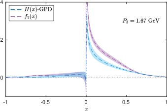
Figure 1: $H$-GPD (blue band) and unpolarized PDF (violet band) for $P_{3}=1.67$ GeV and zero skewness.

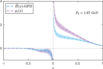
Figure 2: $\widetilde{H}$-GPD (blue band) and helicity PDF (violet band) for $P_{3}=1.67$ GeV and zero skewness.

Our final results for $P_{3}=1.67$ GeV, $t=-0.69$ GeV², and zero skewness are shown in Fig. 1 and Fig. 2 for the unpolarized and helicity GPDs, respectively. For each case, we compare the GPDs with the corresponding PDFs, that is $f_{1}(x)$ for the unpolarized, and $g_{1}(x)$ for the helicity. We observe that the GPDs are suppressed in magnitude as compared to their respective PDFs for all values of $x\lesssim 0.7$. In fact, $\widetilde{H}$-GPD has a steeper slope at small $x$ values. The smaller magnitude of the GPDs is a feature also observed in the standard FFs, which decay with increasing $-t$. For the large-$x$ region, both distributions decay to zero in the same way. The large-$x$ behavior of the unpolarized GPD is in agreement with the power counting analysis of Ref. Yuan (2004). For the antiquark region, we find that the GPDs are compatible with the corresponding PDFs. We note that the statistical uncertainties of GPDs are similar to the PDFs, allowing for such qualitative comparison.

The extraction of the GPDs for $\xi\neq 0$ differs from the one for $\xi=0$, as a different matching kernel is required. Also, unlike the $\xi=0$ case, both helicity GPDs contribute to the matrix element, and therefore a decomposition is required. The comparison between the zero and non-zero skewness is shown in Fig. 3 and Fig. 4, for $P_{3}=1.25$ GeV. The main feature of the GPDs at $\xi\neq 0$ is that an ERBL region ($|x|<1/3$ in our case) appears, differentiating it from the DGLAP region ($|x|>1/3$). The behavior of the GPDs as a function of $t$ for a fixed $x$ is as expected; increasing $-t$ suppresses the GPDs.

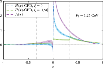
Figure 3: $H$-GPD for $\xi=0$ (blue band) and $\xi=|1/3|$ (green band), as well as the unpolarized PDF (violet band) for $P_{3}=1.25$ GeV. The area between the vertical dashed lines is the ERBL region.

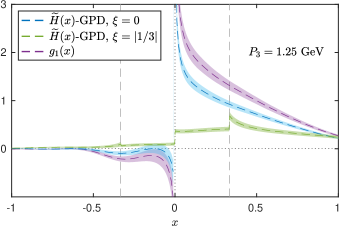
Figure 4: $\widetilde{H}$-GPD for $\xi=0$ (blue band) and $\xi=|1/3|$ (green band), as well as the helicity PDF (violet band) for $P_{3}=1.25$ GeV. The area between the vertical dashed lines is the ERBL region.

Concluding remarks. We presented first results on the unpolarized and helicity GPDs for the proton, employing the quasi-distribution approach, which has been very successful for the extraction of PDFs within lattice QCD. In the case of GPDs, a non-zero momentum is transferred between boosted initial and final states. The lattice QCD data were renormalized non-perturbatively, and the Backus-Gilbert method was used to extract the $x$-dependence of quasi-GPDs. Applying matching to the latter within the LaMET approach yielded the light-cone GPDs in the ${\overline{\rm MS}}$ scheme at 2 GeV.

The momentum dependence of GPDs for $P_{3}=0.83,\,1.25,\,1.67$ GeV at fixed $t{=}-0.69$ GeV² (Figs. S8, S9 of the supplementary material) indicates convergence between the largest two momenta. Our final results, given in Figs. 1-2 at zero skewness and Figs. 3-4 at nonzero skewness, are reassuring, as with increasing $-t$, the magnitude of GPDs is suppressed. With our calculation, we demonstrate that extracting GPDs with controlled statistical uncertainties is feasible. Their accuracy permits qualitative comparison with their corresponding PDFs.

In the near future, we will investigate systematic uncertainties, as studied for PDFs Alexandrou et al. (2019a). The pion mass dependence will also be studied using an ensemble with quark masses fixed to their physical values. In a follow-up calculation, we will also explore the transversity GPD, for which there are two additional form factors, leading to a more evolved decomposition. This makes the disentanglement of the transversity GPDs more challenging.

The current work demonstrates the feasibility of the quasi-distributions approach for GPDs using computational resources that are within reach. However, there is still a long way, until statistical and systematic uncertainties become under control. Extracting GPDs within the first principles formulation of lattice QCD can potentially be combined with future experimental data within the global fits framework. This direction is very timely, as GPDs are at the heart of planned experiments at JLab Biselli (2017) and the Electron-Ion-Collider (EIC) Accardi et al. (2016). Therefore, GPDs are the objects to drive the efforts of the nuclear and hadronic physics communities for the next decades.

Appendix A SUPPLEMENTARY MATERIAL

A.1 Lattice Methods

The work is based on the calculation of proton matrix elements of the nonlocal operator containing a Wilson line in the $z$ direction, $W(0,z)$, that is

$$h_{\Gamma}(z,P_{3},t)\equiv\langle N(P_{f})|\bar{\psi}\left(z\right)\Gamma W(0,z)\psi\left(0\right)|N(P_{i})\rangle\,.$$ (S1)

An important requirement of the quasi-distribution approach is that the hadron is boosted with a momentum in the same direction as the Wilson line, therefore $\mathbf{P}=(0,0,P_{3})$. GPDs are multidimensional objects and require momentum transfer between the initial and final states. In Euclidean space, this is defined as $Q^{2}$, which is related to its Minkowski counterpart as $t\equiv-Q^{2}$. An important parameter of GPDs is the skewness, which is proportional to the momentum transfer in the direction of the boost. In the quasi-distribution method, the relevant quantity is the quasi-skewness defined as $\xi\equiv-\frac{Q_{3}}{2P_{3}}$.

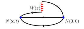
Figure S1: Connected diagram for the evaluation of the three-point function. The initial and final states for the proton are indicated by $N(\mathbf{0},0)$ and $N(\mathbf{x},t)$, respectively.

We calculate the isovector flavor combination, which requires calculation of only the connected diagram shown in Fig. S1. To obtain the ground state of the matrix element, one must calculate two-point and three-point correlation functions,

$$C^{\rm 2pt}(\mathbf{P},t,0)={{\cal P}_{0}}_{\alpha\beta}\sum_{\mathbf{x}}e^{-i\mathbf{P}\cdot\mathbf{x}}\langle 0|N_{\alpha}(\mathbf{x},t)N_{\beta}(\mathbf{0},0)|0\rangle\,,$$ (S2)

$$C_{\Gamma}^{\rm 3pt}(\mathbf{P_{f}},\mathbf{P_{i}};t,\tau,0)={{\cal P}_{\kappa}}_{\alpha\beta}\,\sum_{\mathbf{x},\mathbf{y}}\,e^{i(\mathbf{P_{f}}-\mathbf{P_{i}})\cdot\mathbf{y}}\,e^{-i\mathbf{P_{f}}\cdot\mathbf{x}}\langle 0|N_{\alpha}(\mathbf{x},t)\mathcal{O}_{\gamma^{j}\,\gamma^{5}}(\mathbf{y},\tau;z)N_{\beta}(\mathbf{0},0)|0\rangle\,,$$ (S3)

where $N_{\alpha}(x){=}\epsilon^{abc}u^{a}_{\alpha}(x)\left(d^{b^{T}}(x)\mathcal{C}\gamma_{5}u^{c}(x)\right)$ is the interpolating field for the proton, $\tau$ is the current insertion time. Without loss of generality, we take the source to be at $(\mathbf{0},0)$. ${\cal P}_{0}$ is the parity plus projector ${\cal P}_{0}{=}\frac{1{+}\gamma_{4}}{2}$, and ${\cal P}_{\kappa}$ is either ${\cal P}_{0}$ or ${\cal P}_{\kappa}=\frac{1}{4}(1+\gamma^{0})i\gamma^{5}\gamma^{j}$ if $\kappa$ is spatial. For nonzero momentum transfer, one must form an optimized ratio in order to cancel the time dependence in the exponentials and the overlaps between the interpolating field and the nucleon states,

$$R_{\Gamma}({\cal P}_{\kappa},\mathbf{P_{f}},\mathbf{P_{i}};t,\tau)=\frac{C_{\Gamma}^{3pt}({\cal P}_{\kappa},\mathbf{P_{f}},\mathbf{P_{i}};t,\tau\ )}{C^{2pt}({\cal P}_{0},\mathbf{P_{f}};t)}\times\sqrt{\frac{C^{2pt}({\cal P}_{0},\mathbf{P_{i}};t-\tau)C^{2pt}({\cal P}_{0},\mathbf{P_{f}};\tau)C^{2pt}({\cal P}_{0},\mathbf{P_{f}};t)}{C^{2pt}({\cal P}_{0},\mathbf{P_{f}};t-\tau)C^{2pt}({\cal P}_{0},\mathbf{P_{i}};\tau)C^{2pt}({\cal P}_{0},\mathbf{P_{i}};t)}}\,.$$ (S4)

In the limit $(t_{s}-\tau)\gg a$ and $\tau\gg a$, the ratio of Eq.(S4) becomes time-independent and the ground state matrix element is extracted from a constant fit in the plateau region, that is

$$R_{\Gamma}({\cal P}_{\kappa};\mathbf{P_{f}},\mathbf{P_{i}};t;\tau)\xrightarrow[\tau\gg a]{t-\tau\gg a}\Pi_{\Gamma}({\cal P}\kappa;\mathbf{P_{f}},\mathbf{P_{i}})\,.$$ (S5)

The ground state contribution, $\Pi_{\Gamma}$, is decomposed as shown in Eqs. (2) - (3) of the main text. The expressions for the unpolarized and helicity cases for the non-vanishing projectors can be written as

$${\Pi_{\gamma^{0}}({\cal P}_{0};{P_{f}},{P_{i}})} = C\Bigg{[}F_{H}(Q^{2})\left(\frac{E_{f}E_{i}}{2m^{2}}+\frac{E_{f}+E_{i}}{4m}+\frac{{P_{f}}_{\rho}\,{P_{i}}_{\rho}}{4m^{2}}+\frac{1}{4}\right)$$ (S6)

$$\hskip 11.38092pt+F_{E}(Q^{2})\left({P_{f}}_{\rho}\,{P_{i}}_{\rho}\left(\frac{E_{f}+E_{i}}{8m^{3}}+\frac{1}{4m^{2}}\right)-\frac{(E_{f}-E_{i})^{2}}{8m^{2}}+\frac{E_{f}+E_{i}}{8m}+\frac{1}{4}\right)\Bigg{]}\,,$$

$${\Pi_{\gamma^{0}}({\cal P}_{j};{P_{f}},{P_{i}})} = i\,\epsilon_{j\,0\,\rho\,\tau}C\Bigg{[}F_{H}(Q^{2})\frac{{P_{f}}_{\rho}\,{P_{i}}_{\tau}}{4m^{2}}+F_{E}(Q^{2})\left(\frac{(E_{f}+E_{i}){P_{f}}_{\rho}\,{P_{i}}_{\tau}}{8m^{3}}+\frac{{P_{f}}_{\rho}\,{P_{i}}_{\tau}-{P_{f}}_{\tau}\,{P_{i}}_{\rho}}{8m^{2}}\right)\Bigg{]}\,,$$ (S7)

$${\Pi_{\gamma^{3}\gamma^{5}}({\cal P}_{j};{P_{f}},{P_{i}})} = i\,C\,\Bigg{[}F_{\widetilde{H}}(Q^{2})\left(\delta_{j3}\left(\frac{E_{f}+E_{i}}{4m}-\frac{{P_{f}}_{\rho}\,\,{P_{i}}_{\rho}}{4m^{2}}+\frac{1}{4}\right)+\frac{{P_{i}}_{3}\,\,{P_{f}}_{j}+{P_{f}}_{3}\,\,{P_{i}}_{j}}{4m^{2}}\right)\,\,\,\,\,\,\,\,\,$$ (S8)

$$\hskip 14.22636pt-F_{\widetilde{E}}(Q^{2})\frac{({P_{f}}_{3}-{P_{i}}_{3})(-E_{f}{P_{i}}_{j}+E_{i}{P_{f}}_{j}+m({P_{f}}_{j}-{P_{i}}_{j}))}{8m^{3}}\Bigg{]}\,,$$

where $C=\frac{2m^{2}}{\sqrt{E_{f}E_{i}(E_{f}+m)(E_{i}+m)}}$, with $E_{i,f}=\sqrt{m^{2}+\mathbf{P}_{i,f}^{\,2}}$ . The index $j$ runs only over the spatial components, while a sum over all 4 components is implied for $\rho$ and $\tau$.

To improve the overlap with the proton ground state, we construct the proton interpolating field using momentum-smeared quark fields Bali et al. (2016), on APE smeared gauge links Albanese et al. (1987). The momentum smearing technique was proven to be crucial to suppress statistical uncertainties for matrix elements with boosted hadrons, and in particular for nonlocal operators Alexandrou et al. (2017a). In this work, we can reach $P_{3}=1.67$ GeV at a reasonable computational cost. The momentum smearing function $\mathcal{S}$ on a quark field, $\psi$, reads

$$\mathcal{S}\psi(x)=\frac{1}{1+6\alpha_{G}}\left(\psi(x)+\alpha_{G}\sum_{j=1}^{3}U_{j}(x)e^{i\overline{\xi}\mathbf{P}\cdot\mathbf{j}}\psi(x+\hat{\mathbf{j}})\right),$$ (S9)

where $\alpha_{G}$ is the parameter of the Gaussian smearing Gusken (1990); Alexandrou et al. (1994), $U_{j}$ is the gauge link in the spatial $j$-direction. $\mathbf{P}=(P_{1},P_{2},P_{3})$ is the momentum of the proton (either at the source, or at the sink) and $\overline{\xi}$ is a free parameter that can be tuned so that a maximal overlap with the proton boosted state is achieved. For $\overline{\xi}=0$, Eq. (S9) reduces to the Gaussian smearing function. In our implementation, we keep $\overline{\xi}\mathbf{P}$ parallel to the proton momentum at the source and at the sink. Such a constraint requires separate quark propagators for every momentum transfer, because the gauge links are modified every time by a different complex phase. However, this strategy avoids potential problems due to rotational symmetry breaking. It also has the benefit that every correlator entering the ratio of Eq. (S4) is optimized separately.

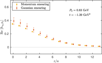
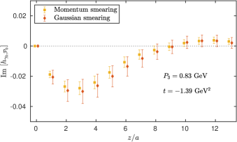
Figure S2: Bare matrix elements obtained for the Dirac insertion $\gamma_{0}$, using the unpolarized parity projector, $\Gamma_{0}$. The data with momentum smearing are shown with yellow squares, while the data using the plain Gaussian smearing are shown with red diamonds. The data correspond to $P_{3}=0.83$ GeV and $t=-1.39$ GeV².

As an example, we show in Fig. S2 the bare matrix elements of the vector operator with and without momentum smearing. For this comparison, we use the unpolarized parity projector, momentum boost $P_{3}=0.83$ GeV, and momentum transfer $t=-1.39$ GeV². The individual components of the momentum transfer are given by the vector $\vec{Q}\frac{L}{2\pi}=(0,-2,2)$. The number of measurements is 1616 for $t_{s}=8a$, and the data using the momentum smearing correspond to $\overline{\xi}=0.6$ after optimization. As can be seen, the use of momentum smearing significantly decreases the statistical uncertainties for both the real and imaginary parts of the matrix elements. In particular, the statistical accuracy increases by a factor of 4-5 in the real part, and 2-3 in the imaginary part, depending on the value of $z$.

In Table SI, we summarize the statistics for each value of the nucleon momentum $P_{3}$, the momentum transfer squared $t$, and skewness $\xi$. In Table SII, we give the numbers of measurements for the corresponding PDFs, to which the computed GPDs can be compared.

$P_{3}$ [GeV]	$\quad\vec{Q}\times\frac{L}{2\pi}\quad$	$-t$ [GeV2]	$\xi$	$N_{\rm confs}$	$N_{\rm meas}$
0.83	(0,2,0)	0.69	0	519	4152
1.25	(0,2,0)	0.69	0	1315	42080
1.67	(0,2,0)	0.69	0	1753	112192
1.25	(0,2,2)	1.39	1/3	417	40032
1.25	(0,2,-2)	1.39	-1/3	417	40032

Table SI: Statistics for both unpolarized and helicity GPDs, at each momentum boost, momentum transfer and skewness.

$P_{3}$ [GeV]	$\Gamma$	$N_{\rm confs}$	$N_{\rm meas}$
0.83	$\gamma_{0}$	115	920
	$\gamma_{5}\gamma_{3}$	194	1560
1.25	$\gamma_{0}$, $\gamma_{5}\gamma_{3}$	731	11696
1.67	$\gamma_{0}$, $\gamma_{5}\gamma_{3}$	1644	105216

Table SII: Statistics for the unpolarized and helicity PDFs at the three nucleon momenta. The Dirac structures used in three-point functions calculations are $\Gamma=\gamma_{0}$ and $\Gamma=\gamma_{5}\gamma_{3}$ for the unpolarized and helicity distributions, respectively.

A.2 Renormalization

We employ an RI-type renormalization prescription, using the momentum source method Gockeler et al. (1999); Alexandrou et al. (2017d) that offers high statistical accuracy. The appropriate conditions for the renormalization functions of the nonlocal operator, $Z_{\Gamma}$, and the quark field, $Z_{q}$, are

$$Z_{q}^{-1}\,Z_{\Gamma}(z) {\rm Tr}\left[{\cal V}_{\Gamma}(p,z)\,\not{p}\right]\Bigr{|}_{p^{2}{=}\mu_{0}^{2}}={\rm Tr}\left[{\cal V}_{\Gamma}^{{\rm Born}}(p,z)\,\not{p}\right]\Bigr{|}_{p^{2}{=}\mu_{0}^{2}}\,,$$ (S11)

$$Z_{q}=\frac{1}{12}{\rm Tr}\left[(S(p))^{-1}\,S^{\rm Born}(p)\right]\Bigr{|}_{p^{2}=\mu_{0}^{2}}\,.$$

Note that Eq. (S11) is applied at each value of $z$ separately. ${\cal V}(p,z)$ ($S(p)$) is the amputated vertex function of the operator (fermion propagator) and $S^{{\rm Born}}(p)$ is the tree-level of the propagator.

The above prescription is mass-independent, and therefore $Z_{\Gamma}$ do not depend on the quark mass. However, there might be residual cut-off effects of the form $am_{q}$. To eliminate any systematic related to such effects, we extract $Z_{\Gamma}$ using multiple degenerate-quark ensembles ($N_{f}=4$) at the same lattice spacing and action as the $N_{f}=2+1+1$ ensemble used for the production of the nucleon matrix elements. We then take the chiral limit of the $Z_{\Gamma}$. The exact procedure is described in detail in Ref. Alexandrou et al. (2019a). We use five $N_{f}=4$ ensembles as given in Tab. SIII, which have been produced for the calculation of the renormalization functions at the same $\beta$ value as the $N_{f}=2+1+1$ ensemble used for the extraction of the matrix elements of Eq. (S1).

$\beta=1.726$,	$c_{\rm SW}=1.74$,	$a=0.093$ fm
$24^{3}\times 48$	$\,\,a\mu=0.0060$	$\,\,m_{\pi}=357.84$ MeV
$24^{3}\times 48$	$\,\,a\mu=0.0080$	$\,\,m_{\pi}=408.11$ MeV
$24^{3}\times 48$	$\,\,a\mu=0.0100$	$\,\,m_{\pi}=453.48$ MeV
$24^{3}\times 48$	$\,\,a\mu=0.0115$	$\,\,m_{\pi}=488.41$ MeV
$24^{3}\times 48$	$\,\,a\mu=0.0130$	$\,\,m_{\pi}=518.02$ MeV

Table SIII: Parameters of the $N_{f}=4$ ensembles used for the calculation of the renormalization functions.

The RI renormalization scale $\mu_{0}$, defined in Eq. (S11), is chosen appropriately to have suppressed discretization effects, as explained in Ref. Alexandrou et al. (2017d). We employ several values that have the same spatial components, that is $p=(p_{0},p_{1},p_{1},p_{1})$, so that the ratio $\frac{p^{4}}{(p^{2})^{2}}$ is less than 0.35, as suggested in Ref. Constantinou et al. (2010). In this work, we use different values of $\mu_{0}$ ($(a\,\mu_{0})^{2}\in[1,5]$) to check the dependence of the matching formalism on $\mu_{0}$. For each $\mu_{0}$ value, we apply a chiral extrapolation using the fit

$$Z^{\rm RI}_{\Gamma}(z,\mu_{0},m_{\pi})={Z}^{\rm RI}_{{\Gamma},0}(z,\mu_{0})+m_{\pi}^{2}\,{Z}^{\rm RI}_{{\Gamma},1}(z,\mu_{0})\,,$$ (S12)

to extract the mass-independent ${Z}^{\rm RI}_{{\Gamma},0}(z,\mu_{0})$.

As mentioned in the main text, the matching kernel of Ref. Liu et al. (2019) requires that the quasi-GPDs are renormalized in the RI scheme. For consistency, we use the same for $\xi=0$ and use the renormalization functions defined on a single ${\rm RI}$ renormalization scale, $(a\mu_{0})^{2}\approx 1.17$. This scale also enters the matching equations. We find negligible dependence when varying $\mu_{0}$.

A.3 Reconstruction of $x$-dependence

The renormalized matrix elements $F_{G}$, where $G=H,E$, are related to the quasi-distributions $G_{q}$ by a Fourier transform:

$$F_{G}(z,P_{3},t,\xi,\mu_{0})=\int_{-\infty}^{\infty}dx\,e^{ixP_{3}z}\,G_{q}(x,t,\xi,\mu_{0},P_{3})\,.$$ (S13)

Inverting this expression relates the quasi-GPDs to the matrix elements. However, the inverse equation involves a Fourier transform over a continuum of lengths of the Wilson line, up to infinity, while the lattice provides only a discrete set of determinations of $F_{G}$, for integer values of $z/a$ up to roughly half of the lattice extent in the boost direction, $L/2a$. Thus, the inversion of Eq. (S13) poses a mathematically ill-defined problem, as argued and discussed in detail in Ref. Karpie et al. (2018). The inverse problem originates from incomplete information, i.e. attempting to reconstruct a continuous distribution from a finite number of input data points. As such, its solution necessarily requires making additional assumptions that provide the missing information. These assumptions should be as mild as possible and preferably model-independent – else, the reconstructed distribution may be biased.

One of the approaches proposed in Ref. Karpie et al. (2018) is to use the Backus-Gilbert (BG) method Backus and Gilbert (1968). The model-independent criterion used in the BG procedure, to choose from among the infinitely many possible solutions to the inverse problem, is that the variance of the solution with respect to the statistical variation of the input data should be minimal. The reconstruction proceeds separately for each value of the momentum fraction $x$. In practice, we separate the exponential of the Fourier transform into its cosine and sine parts, related to the real and imaginary parts of the matrix elements, respectively. We define a vector $\textbf{a}_{K}(x)$, where $K$ denotes either the cosine or sine kernel, of dimension $d$ equal to the number of available input matrix elements, i.e. $d=z_{\rm max}/a+1$, where $z_{\rm max}/a$ is the maximum length of the Wilson line (in lattice units) used to determine the quasi-distribution. The BG procedure consists in finding the vectors $\textbf{a}_{K}(x)$ for both kernels according to the variance minimization criterion. The vector $\textbf{a}_{K}(x)$ is an approximate inverse of the cosine/sine kernel function $K(x)$, that is:

$$\Delta(x-x^{\prime})=\sum_{z/a=0}^{d-1}a_{K}(x)_{z/a}K(x^{\prime})_{z/a}\,,$$ (S14)

and $K(x^{\prime})_{z/a}=\cos(x^{\prime}P_{3}z)$ or $K(x^{\prime})_{z/a}=\sin(x^{\prime}P_{3}z)$ are elements of a $d$-dimensional vector of discrete kernel values corresponding to available integer values of $z/a$. The function $\Delta(x-x^{\prime})$ is, thus, an approximation to the Dirac delta function $\delta(x-x^{\prime})$, with the quality of this approximation depending, in practice, on the achievable dimension $d$ at given simulation parameters.

The vectors $\textbf{a}_{K}(x)$ are found from optimization conditions resulting from the BG criterion. We refer to Ref. Karpie et al. (2018) for their explicit form and here, we just summarize the final result. We define a $d\times d$-dimensional matrix $\textbf{M}_{K}(x)$, with matrix elements

$$M_{K}(x)_{z/a,z^{\prime}/a}=\int_{0}^{x_{c}}dx^{\prime}\,(x-x^{\prime})^{2}K(x^{\prime})_{z/a}\,K(x^{\prime})_{z^{\prime}/a}+\rho\,\delta_{z/a,z^{\prime}/a}\,,$$ (S15)

where $x_{c}$ is the maximum value of $x$ for which the quasi-distribution is taken to be non-zero (i.e. its reconstruction proceeds for $x\in[0,x_{c}]$) and the parameter $\rho$ regularizes the matrix $\textbf{M}_{K}$. This regularization, proposed by Tikhonov Tikhonov (1963), was put up as one possible way of making $\textbf{M}_{K}$ invertible Ulybyshev et al. (2018, 2017); Karpie et al. (2018)). The value of $\rho$ determines the resolution of the method and should be taken as rather small, in order to avoid a bias. We use $\rho=10^{-3}$, which leads to reasonable resolution and is large enough to avoid oscillations in the final distributions related to the presence of small eigenvalues of $\textbf{M}_{K}$. Additionally, we define a $d$-dimensional vector $\textbf{u}_{K}$, with elements

$$u_{K;z/a}=\int_{0}^{x_{c}}dx^{\prime}\,K(x^{\prime})_{z/a}.$$ (S16)

The above mentioned optimization conditions lead to:

$$\textbf{a}_{K}(x)=\frac{\textbf{M}_{K}^{-1}(x)\,\textbf{u}_{K}}{\textbf{u}_{K}^{T}\,\textbf{M}_{K}^{-1}(x)\,\textbf{u}_{K}}$$ (S17)

and the final BG-reconstructed quasi-distributions are given by

$$G_{q}(x,t,\xi,\mu_{0},P_{3})=\frac{1}{2}\sum_{z/a}\left(a_{\rm cos}(x)_{z/a}\,{\rm Re}\,F_{G}(z,P_{3},t,\xi)+a_{\rm sin}(x)_{z/a}\,{\rm Im}\,F_{G}(z,P_{3},t,\xi)\right)\,.$$ (S18)

A.4 Matching Procedure

Contact between the physical distributions and the quasi-GPDs is established through a perturbative matching procedure. The factorization formula for the Dirac structure $\Gamma$ takes the form

$$G_{q}(x,t,\xi,\mu_{0},(\mu_{0})_{3},P_{3}) = \int_{-1}^{1}\frac{dy}{|y|}\,C_{G}\left(\frac{x}{y},\frac{\xi}{y},\frac{\mu}{yP_{3}},\frac{(\mu_{0})_{3}}{yP_{3}},r\right)G(y,t,\xi,\mu)+\mathcal{O}\left(\frac{m^{2}}{P_{3}^{2}},\frac{t}{P_{3}^{2}},\frac{\Lambda_{\rm QCD}^{2}}{x^{2}P_{3}^{2}}\right),$$ (S19)

where $C_{G}$ is the matching kernel, known to one-loop level in perturbation theory, and the involved renormalization scales are: $\mu_{0}$ – RI renormalization scale, its $z$-component $(\mu_{0})_{3}$ (with $r=\mu_{0}^{2}/(\mu_{0})_{3}^{2}$), and $\mu$ – final ${\overline{\rm MS}}$ scale. This formula establishes that quasi-distributions are equal to light-cone distributions up to power-suppressed corrections (nucleon mass ($m$) corrections and higher-twist corrections). The matching coefficient for the GPDs, was first derived for flavor non-singlet unpolarized and helicity quasi-GPDs in Ref. Ji et al. (2015) and for transversity quasi-GPDs in Ref. Xiong and Zhang (2015), using the transverse momentum cutoff scheme. Recently, a matching formula was also derived for all Dirac structures Liu et al. (2019) relating quasi-GPDs renormalized in a variant of the RI/MOM scheme to ${\overline{\rm MS}}$ light-cone PDFs. In these calculations, it was shown that the matching for GPDs at zero skewness is the same as for PDFs. It was also demonstrated that, to one-loop level, the $H$-type and $E$-type GPDs have the same matching formula. The matching kernel for a given Dirac structure $\Gamma$ and parton momentum $p_{3}$ reads

$$C_{G}\left(\Gamma;x,\xi,\frac{p_{3}}{\mu},\frac{p_{3}}{(\mu_{0})_{3}},r\right)=\delta(x-1) +\frac{\alpha_{s}C_{F}}{2\pi}\left\{\begin{array}[]{lc}G_{1}(\Gamma;x,\xi)_{+}&x<-\xi\\ G_{2}(\Gamma;x,\xi,p_{3}/\mu)_{+}&|x|<\xi\\ G_{3}(\Gamma;x,\xi,p_{3}/\mu)_{+}&\xi<x<1\\ -G_{1}(\Gamma;x,\xi)_{+}&x>1\end{array}\right.$$ (S24)

$$-\frac{\alpha_{s}C_{F}}{2\pi}\left|\frac{p_{3}}{(\mu_{0})_{3}}\right|f_{\not{p}}\left(\Gamma;\frac{p_{3}}{(\mu_{0})_{3}}(x-1)+1,r\right)_{+},$$ (S25)

The functions $G_{1},G_{2},G_{3}$ for the matching of bare quasi-GPDs can be found in Ref. Liu et al. (2019), while the one-loop RI counterterm $f_{\not{p}}$ for the variant that we employ (RI-$\not{p}$) is given in Ref. Liu et al. (2020). The plus prescription is defined as

$$f(x)_{+}=f(x)+\delta(x-1)\int dyf(y)$$ (S26)

and it combines the so-called ”real” (vertex) and ”virtual” (self-energy) corrections.

A.5 Results

In this section, we provide more details for the extracted matrix elements and the final GPDs.

In Fig. S3, we show the bare matrix elements for the vector operator, using the projectors ${\cal P}_{0}$ ($h_{\gamma_{0},{\cal P}_{0}}$) and ${\cal P}_{1}$ with $\kappa=1$ ($h_{\gamma_{0},{\cal P}_{1}}$). Note that for the polarized projector, only $\kappa=1$ contributes, as the momentum transfer has zero component in that direction. Focusing on the largest value of the momentum $P_{3}=1.67$ GeV, one observes that both $h_{\gamma_{0},{\cal P}_{0}}$ and $h_{\gamma_{0},{\cal P}_{1}}$ give similar contributions. The decomposition of the renormalized matrix elements leads to $F_{H}$ and $F_{E}$, shown in Fig. S4. It is interesting to observe that the statistical errors for $F_{E}$ are, in general, larger than those for $F_{H}$. This effect has its origin in the kinematic coefficients of $F_{E}$ in the decomposition of the matrix element. We find that the momentum dependence changes based on the values of $z$, and on the quantity under study. This momentum dependence propagates in a nontrivial way to the final $H$- and $E$-GPDs, as one has to reconstruct the quasi-GPDs in momentum space, and then, apply the appropriate matching formula, which depends on the momentum $P_{3}$.

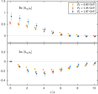
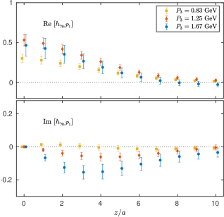
Figure S3: The bare matrix elements $h_{\gamma_{0}}$ using parity projector ${\cal P}_{0}$ (left panels) and ${\cal P}_{1}$ (right panels) for zero skewness and $t=-0.69$ GeV². The top (bottom) plots correspond to the real (imaginary) part of the matrix elements. Momenta $P_{3}=0.83,\,1.25,\,1.67$ GeV are shown with orange squares, red diamonds, blue circles, respectively.

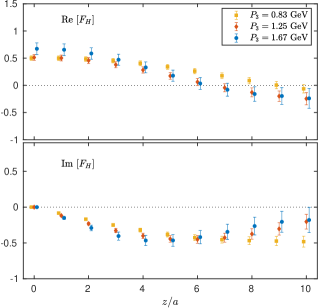
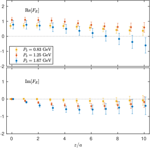
Figure S4: The renormalized quantities $F_{H}$ (left panels) and $F_{E}$ (right panels) for $t=-0.69$ GeV² and $\xi=0$. The top (bottom) plots correspond to the real (imaginary) part of the matrix elements. Momenta $P_{3}=0.83,\,1.25,\,1.67$ GeV are shown with orange squares, red diamonds, blue circles, respectively.

In Fig. S4 we show the decomposed quantities $F_{H}$ and $F_{E}$, which have been disentangled using the renormalized matrix elements $h_{\gamma^{0},{\cal P}_{0}}$ and $h_{\gamma^{0},{\cal P}_{1}}$. We find negligible momentum dependence in ${\rm Re}[F_{H}]$ for $0<z<5$, while it has a steeper and compatible slope for the two largest momenta in the region $5\leq z\leq 9$. ${\rm Re}[F_{H}]$ flattens out for all three momenta for $z\geq 10$, which are consistent. Similarly, ${\rm Im}[F_{H}]$ is compatible for the largest two momenta for all values of $z$, while the lowest momentum evinces a clearly slower decay to zero. This might indicate onset of convergence above $P_{3}=1.25$ GeV. Note, however, that the matching depends on $P_{3}$ and thus, more conclusions about convergence can be drawn after applying this procedure. For ${\rm Re}[F_{E}]$, the errors are significantly larger than for ${\rm Re}[F_{H}]$, as remarked above, and we observe somewhat slower decay at $P_{3}=1.25$ GeV as compared to $P_{3}=1.67$ GeV. This may indicate slower convergence in the $E$-GPD, but may also be a statistical effect, since ${\rm Im}[F_{E}]$ is, again, compatible for the largest two boosts. Similarly to ${\rm Re}[F_{H}]$, ${\rm Re}[F_{E}]$ also approaches zero for $z\geq 6$. Finally, we find that ${\rm Im}[F_{E}]$ has very small contribution for the lowest momentum, while it is enhanced in the intermediate $z$ region for the largest two boosts and comparable in magnitude to ${\rm Im}[F_{H}]$.

The matrix element $h_{\gamma^{3}\gamma^{5}}$ is shown in the left panel of Fig. S5 for $t=-0.69$ GeV² and $\xi=0$. The corresponding $F_{\widetilde{H}}$ is shown in the right panel. We note that for zero skewness, the kinematic factor of $\widetilde{E}$ is zero, and we only extract $\widetilde{H}$ from the lattice QCD data. We observe that both for the real and the imaginary part of $F_{\widetilde{H}}$, there are significant differences between the largest two momenta. Thus, we postpone conclusions about convergence to the discussion of the final GPDs.

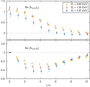
Figure S5: Left panels: The bare matrix elements $h_{\gamma_{3}\gamma^{5}}$ using parity projector ${\cal P}_{3}$ for $t=-0.69$ GeV² and $\xi=0$. Right panels: The renormalized $F_{\widetilde{H}}$. The top (bottom) plots correspond to the real (imaginary) part of the matrix elements. Momenta $P_{3}=0.83,\,1.25,\,1.67$ GeV are shown with orange squares, red diamonds, blue circles, respectively.

.

It is interesting to compare the matrix elements at fixed $P_{3}$ for different values of the skewness, and therefore, different values of $t$. In Fig. S6, we show $F_{H}$ and $F_{E}$ at $P_{3}=1.25$ GeV, with $\{t,\xi\}=\{$-0.69 GeV${}^{2},0\}$ and $\{t,\xi\}=\{$-1.39 GeV${}^{2},1/3\}$. The real part of $F_{E}$ shows the largest sensitivity to such a simultaneous change of $t$ and $\xi$. In addition, the imaginary part of $F_{H}$ shows significant dependence on $\{t,\xi\}$ for $z/a>3$. The case of $\widetilde{F}_{H}$ is shown in the left panel of Fig. S7, where we observe large differences between $\{t,\xi\}=\{$-0.69 GeV${}^{2},0\}$ and $\{t,\xi\}=\{$-1.39 GeV${}^{2},1/3\}$. For completeness, we show $\widetilde{F}_{E}$ for $\xi=1/3$ in the right panel of Fig. S7.

Figure S6: Renormalized quantities $F_{H}$ and $F_{E}$ for $P_{3}=1.25$ GeV, at $t=-0.69$ GeV², $\xi=0$ (red squares) and $t=-1.39$ GeV², $\xi=|1/3|$ (green diamonds).

Figure S7: Renormalized $F_{\widetilde{H}}$ and $F_{\widetilde{E}}$ for $P_{3}=1.25$ GeV, at $t=-0.69$ GeV², $\xi=0$ (red squares) and $t=-1.39$ GeV², $\xi=|1/3|$ (green diamonds).

We now move on to the discussion of the final GPDs, in particular their convergence in momentum for zero skewness ($t=-0.69$ GeV²). We compare the unpolarized GPDs for $P_{3}=0.83,\,1.25,\,1.67$ GeV in Fig. S8. The $H$-GPD has negligible $P_{3}$-dependence for every region of $x$, while the $E$-GPD exibits convergence between the two largest momenta for $x>0$, which is of main interest. We note that the statistical errors on $E$-GPD are larger than those of the $H$-GPD, a feature already observed in $F_{E}$ (see Fig. S3). In Fig. S9, we show the momentum dependence of the $\widetilde{H}$-GPD. We observe that the relatively large differences between the renormalized $F_{\widetilde{H}}$ for the lowest two momenta and $P_{3}=1.67$ GeV are compensated by the matching procedure, indicating final convergence within the reported statistical uncertainties. Thus, this conclusion holds for both the unpolarized and the helicity $H$-GPD.

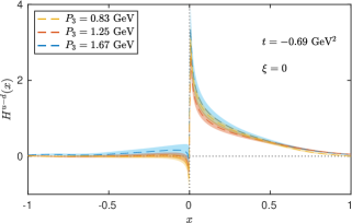
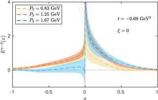
Figure S8: Momentum dependence of final $H$-GPD and $E$-GPD. Results on momenta $P_{3}=0.83,\,1.25,\,1.67$ GeV are shown with orange, red, blue band, respectively.

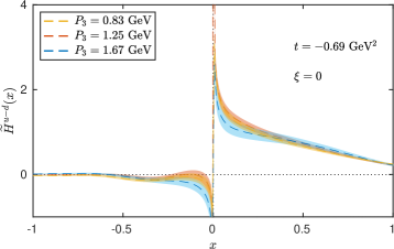
Figure S9: Momentum dependence of final $\widetilde{H}$-GPD using results for $P_{3}=0.83,\,1.25,\,1.67$ GeV, shown with orange, red, blue band, respectively.

In Fig. S10 we provide a comparison between the $H$- and $E$-GPDs (left panel), and $\widetilde{H}$- and $\widetilde{E}$-GPDs (right panel). In the unpolarized case, $H$- and $E$-GPDs are compatible with each other in the quark region. However, the Pauli FF, corresponding to the $x$-integral of the $E$-GPD, is considerably larger than the Dirac FF (integral of $H$-GPD) at this momentum transfer and this is achieved by the larger values of the $E$-GPD in the antiquark region. For the helicity case, the $\widetilde{E}$-GPD is significantly larger than the $\widetilde{H}$-GPD, which reflects the fact that the axial-vector FF $G_{P}$ is found to be a factor $\approx 3$ larger than the $G_{A}$ at this momentum transfer, in a lattice setup with similar parameters Alexandrou et al. (2013). We also note that the integrals of $H$-,$E$-,$\widetilde{H}$- and $\widetilde{E}$-GPDs extracted in this work are all compatible with their respective FFs obtained in Ref. Alexandrou et al. (2013).

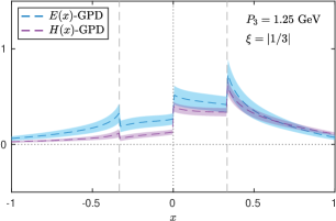
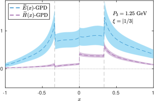
Figure S10: Left: Comparison of $H$-GPD (violet band) and $E$-GPD (blue band) for $P_{3}=,1.25$ GeV and $\xi=1/3$. Right: Same as left plot for helicity GPDs.

References

- Collins et al. (1989) J. C. Collins, D. E. Soper, and G. F. Sterman, Factorization of Hard Processes in QCD (1989), vol. 5, pp. 1–91, eprint hep-ph/0409313.
- Ji (1997a) X.-D. Ji, Phys. Rev. Lett. 78, 610 (1997a), eprint hep-ph/9603249.
- Radyushkin (1996) A. V. Radyushkin, Phys. Lett. B380, 417 (1996), eprint hep-ph/9604317.
- Mueller et al. (1994) D. Mueller, D. Robaschik, B. Geyer, F. M. Dittes, and J. Horejsi, Fortsch. Phys. 42, 101 (1994), eprint hep-ph/9812448.
- Collins (2003) J. C. Collins, Acta Phys. Polon. B34, 3103 (2003), eprint hep-ph/0304122.
- Ji et al. (2005) X.-d. Ji, J.-p. Ma, and F. Yuan, Phys. Rev. D71, 034005 (2005), eprint hep-ph/0404183.
- Collins and Soper (1982) J. C. Collins and D. E. Soper, Nucl. Phys. B 194, 445 (1982).
- Dokshitzer (1977) Y. L. Dokshitzer, Sov. Phys. JETP 46, 641 (1977).
- Gribov and Lipatov (1972) V. Gribov and L. Lipatov, Sov. J. Nucl. Phys. 15, 438 (1972).
- Lipatov (1975) L. Lipatov, Sov. J. Nucl. Phys. 20, 94 (1975).
- Altarelli and Parisi (1977) G. Altarelli and G. Parisi, Nucl. Phys. B 126, 298 (1977).
- Efremov and Radyushkin (1980) A. Efremov and A. Radyushkin, Phys. Lett. B 94, 245 (1980).
- Lepage and Brodsky (1980) G. Lepage and S. J. Brodsky, Phys. Rev. D 22, 2157 (1980).
- Ji (1998) X.-D. Ji, J. Phys. G 24, 1181 (1998), eprint hep-ph/9807358.
- Ji (1997b) X.-D. Ji, Phys. Rev. D 55, 7114 (1997b), eprint hep-ph/9609381.
- Diehl (2003) M. Diehl, Phys. Rept. 388, 41 (2003), eprint hep-ph/0307382.
- Ji (2004) X. Ji, Ann. Rev. Nucl. Part. Sci. 54, 413 (2004).
- Belitsky and Radyushkin (2005) A. V. Belitsky and A. V. Radyushkin, Phys. Rept. 418, 1 (2005), eprint hep-ph/0504030.
- Kumericki et al. (2016) K. Kumericki, S. Liuti, and H. Moutarde, Eur. Phys. J. A 52, 157 (2016), eprint 1602.02763.
- Collins (2011) J. Collins, Camb. Monogr. Part. Phys. Nucl. Phys. Cosmol. 32, 1 (2011).
- Ji (2013) X. Ji, Phys. Rev. Lett. 110, 262002 (2013), eprint 1305.1539.
- Ji (2014) X. Ji, Sci. China Phys. Mech. Astron. 57, 1407 (2014), eprint 1404.6680.
- Xiong et al. (2014) X. Xiong, X. Ji, J.-H. Zhang, and Y. Zhao, Phys.Rev. D90, 014051 (2014), eprint 1310.7471.
- Lin et al. (2015) H.-W. Lin, J.-W. Chen, S. D. Cohen, and X. Ji, Phys. Rev. D91, 054510 (2015), eprint 1402.1462.
- Alexandrou et al. (2015) C. Alexandrou, K. Cichy, V. Drach, E. Garcia-Ramos, K. Hadjiyiannakou, K. Jansen, F. Steffens, and C. Wiese, Phys. Rev. D92, 014502 (2015), eprint 1504.07455.
- Chen et al. (2016) J.-W. Chen, S. D. Cohen, X. Ji, H.-W. Lin, and J.-H. Zhang, Nucl. Phys. B911, 246 (2016), eprint 1603.06664.
- Alexandrou et al. (2017a) C. Alexandrou, K. Cichy, M. Constantinou, K. Hadjiyiannakou, K. Jansen, F. Steffens, and C. Wiese, Phys. Rev. D96, 014513 (2017a), eprint 1610.03689.
- Briceño et al. (2017) R. A. Briceño, M. T. Hansen, and C. J. Monahan, Phys. Rev. D96, 014502 (2017), eprint 1703.06072.
- Constantinou and Panagopoulos (2017) M. Constantinou and H. Panagopoulos, Phys. Rev. D96, 054506 (2017), eprint 1705.11193.
- Alexandrou et al. (2017b) C. Alexandrou, K. Cichy, M. Constantinou, K. Hadjiyiannakou, K. Jansen, H. Panagopoulos, and F. Steffens, Nucl. Phys. B923, 394 (2017b), eprint 1706.00265.
- Ji et al. (2017) X. Ji, J.-H. Zhang, and Y. Zhao, Nucl. Phys. B 924, 366 (2017), eprint 1706.07416.
- Ji et al. (2018) X. Ji, J.-H. Zhang, and Y. Zhao, Phys. Rev. Lett. 120, 112001 (2018), eprint 1706.08962.
- Ishikawa et al. (2017) T. Ishikawa, Y.-Q. Ma, J.-W. Qiu, and S. Yoshida, Phys. Rev. D96, 094019 (2017), eprint 1707.03107.
- Green et al. (2018) J. Green, K. Jansen, and F. Steffens, Phys. Rev. Lett. 121, 022004 (2018), eprint 1707.07152.
- Wang et al. (2018) W. Wang, S. Zhao, and R. Zhu, Eur. Phys. J. C 78, 147 (2018), eprint 1708.02458.
- Stewart and Zhao (2018) I. W. Stewart and Y. Zhao, Phys. Rev. D97, 054512 (2018), eprint 1709.04933.
- Izubuchi et al. (2018) T. Izubuchi, X. Ji, L. Jin, I. W. Stewart, and Y. Zhao, Phys. Rev. D98, 056004 (2018), eprint 1801.03917.
- Alexandrou et al. (2018a) C. Alexandrou, K. Cichy, M. Constantinou, K. Jansen, A. Scapellato, and F. Steffens, Phys. Rev. Lett. 121, 112001 (2018a), eprint 1803.02685.
- Alexandrou et al. (2018b) C. Alexandrou, K. Cichy, M. Constantinou, K. Jansen, A. Scapellato, and F. Steffens, Phys. Rev. D98, 091503 (2018b), eprint 1807.00232.
- Zhang et al. (2019a) J.-H. Zhang, J.-W. Chen, L. Jin, H.-W. Lin, A. Schäfer, and Y. Zhao, Phys. Rev. D100, 034505 (2019a), eprint 1804.01483.
- Briceño et al. (2018) R. A. Briceño, J. V. Guerrero, M. T. Hansen, and C. J. Monahan, Phys. Rev. D 98, 014511 (2018), eprint 1805.01034.
- Spanoudes and Panagopoulos (2018) G. Spanoudes and H. Panagopoulos, Phys. Rev. D 98, 014509 (2018), eprint 1805.01164.
- Liu et al. (2020) Y.-S. Liu et al. (Lattice Parton), Phys. Rev. D 101, 034020 (2020), eprint 1807.06566.
- Radyushkin (2019a) A. Radyushkin, Phys. Lett. B 788, 380 (2019a), eprint 1807.07509.
- Zhang et al. (2019b) J.-H. Zhang, X. Ji, A. Schäfer, W. Wang, and S. Zhao, Phys. Rev. Lett. 122, 142001 (2019b), eprint 1808.10824.
- Li et al. (2019) Z.-Y. Li, Y.-Q. Ma, and J.-W. Qiu, Phys. Rev. Lett. 122, 062002 (2019), eprint 1809.01836.
- Alexandrou et al. (2019a) C. Alexandrou, K. Cichy, M. Constantinou, K. Hadjiyiannakou, K. Jansen, A. Scapellato, and F. Steffens, Phys. Rev. D99, 114504 (2019a), eprint 1902.00587.
- Wang et al. (2019) W. Wang, J.-H. Zhang, S. Zhao, and R. Zhu, Phys. Rev. D 100, 074509 (2019), eprint 1904.00978.
- Chen et al. (2020a) J.-W. Chen, H.-W. Lin, and J.-H. Zhang, Nucl. Phys. B 952, 114940 (2020a), eprint 1904.12376.
- Izubuchi et al. (2019) T. Izubuchi, L. Jin, C. Kallidonis, N. Karthik, S. Mukherjee, P. Petreczky, C. Shugert, and S. Syritsyn, Phys. Rev. D100, 034516 (2019), eprint 1905.06349.
- Cichy et al. (2019) K. Cichy, L. Del Debbio, and T. Giani, JHEP 10, 137 (2019), eprint 1907.06037.
- Wang et al. (2020) W. Wang, Y.-M. Wang, J. Xu, and S. Zhao, Phys. Rev. D 102, 011502 (2020), eprint 1908.09933.
- Son et al. (2020) H.-D. Son, A. Tandogan, and M. V. Polyakov, Phys. Lett. B 808, 135665 (2020), eprint 1911.01955.
- Green et al. (2020) J. R. Green, K. Jansen, and F. Steffens, Phys. Rev. D 101, 074509 (2020), eprint 2002.09408.
- Chai et al. (2020) Y. Chai et al., Phys. Rev. D 102, 014508 (2020), eprint 2002.12044.
- Braun et al. (2020) V. Braun, K. Chetyrkin, and B. Kniehl, JHEP 07, 161 (2020), eprint 2004.01043.
- Bhattacharya et al. (2020a) S. Bhattacharya, K. Cichy, M. Constantinou, A. Metz, A. Scapellato, and F. Steffens (2020a), eprint 2004.04130.
- Bhattacharya et al. (2020b) S. Bhattacharya, K. Cichy, M. Constantinou, A. Metz, A. Scapellato, and F. Steffens, Phys. Rev. D 102, 034005 (2020b), eprint 2005.10939.
- Bhattacharya et al. (2020c) S. Bhattacharya, K. Cichy, M. Constantinou, A. Metz, A. Scapellato, and F. Steffens (2020c), eprint 2006.12347.
- Chen et al. (2020b) L.-B. Chen, W. Wang, and R. Zhu, Phys. Rev. D 102, 011503 (2020b), eprint 2005.13757.
- Chen et al. (2020c) L.-B. Chen, W. Wang, and R. Zhu (2020c), eprint 2006.10917.
- Chen et al. (2020d) L.-B. Chen, W. Wang, and R. Zhu (2020d), eprint 2006.14825.
- Ji et al. (2020a) X. Ji, Y. Liu, A. Schäfer, W. Wang, Y.-B. Yang, J.-H. Zhang, and Y. Zhao (2020a), eprint 2008.03886.
- Liu and Dong (1994) K.-F. Liu and S.-J. Dong, Phys. Rev. Lett. 72, 1790 (1994), eprint hep-ph/9306299.
- Detmold and Lin (2006) W. Detmold and C. J. D. Lin, Phys. Rev. D73, 014501 (2006), eprint hep-lat/0507007.
- Braun and Mueller (2008) V. Braun and D. Mueller, Eur. Phys. J. C55, 349 (2008), eprint 0709.1348.
- Bali et al. (2018a) G. S. Bali et al., Eur. Phys. J. C 78, 217 (2018a), eprint 1709.04325.
- Bali et al. (2018b) G. S. Bali, V. M. Braun, B. Gläßle, M. Göckeler, M. Gruber, F. Hutzler, P. Korcyl, A. Schäfer, P. Wein, and J.-H. Zhang, Phys. Rev. D98, 094507 (2018b), eprint 1807.06671.
- Detmold et al. (2018) W. Detmold, I. Kanamori, C. J. D. Lin, S. Mondal, and Y. Zhao (2018), eprint 1810.12194.
- Liang et al. (2019) J. Liang, T. Draper, K.-F. Liu, A. Rothkopf, and Y.-B. Yang (XQCD) (2019), eprint 1906.05312.
- Ma and Qiu (2018a) Y.-Q. Ma and J.-W. Qiu, Phys. Rev. D98, 074021 (2018a), eprint 1404.6860.
- Ma and Qiu (2015) Y.-Q. Ma and J.-W. Qiu, Int. J. Mod. Phys. Conf. Ser. 37, 1560041 (2015), eprint 1412.2688.
- Radyushkin (2017a) A. Radyushkin, Phys. Lett. B767, 314 (2017a), eprint 1612.05170.
- Chambers et al. (2017) A. J. Chambers, R. Horsley, Y. Nakamura, H. Perlt, P. E. L. Rakow, G. Schierholz, A. Schiller, K. Somfleth, R. D. Young, and J. M. Zanotti, Phys. Rev. Lett. 118, 242001 (2017), eprint 1703.01153.
- Radyushkin (2017b) A. V. Radyushkin, Phys. Rev. D96, 034025 (2017b), eprint 1705.01488.
- Orginos et al. (2017) K. Orginos, A. Radyushkin, J. Karpie, and S. Zafeiropoulos, Phys. Rev. D96, 094503 (2017), eprint 1706.05373.
- Ma and Qiu (2018b) Y.-Q. Ma and J.-W. Qiu, Phys. Rev. Lett. 120, 022003 (2018b), eprint 1709.03018.
- Radyushkin (2018a) A. V. Radyushkin, Phys. Lett. B781, 433 (2018a), eprint 1710.08813.
- Radyushkin (2018b) A. Radyushkin, Phys. Rev. D98, 014019 (2018b), eprint 1801.02427.
- Zhang et al. (2018) J.-H. Zhang, J.-W. Chen, and C. Monahan, Phys. Rev. D 97, 074508 (2018), eprint 1801.03023.
- Karpie et al. (2018) J. Karpie, K. Orginos, and S. Zafeiropoulos, JHEP 11, 178 (2018), eprint 1807.10933.
- Sufian et al. (2019) R. S. Sufian, J. Karpie, C. Egerer, K. Orginos, J.-W. Qiu, and D. G. Richards, Phys. Rev. D99, 074507 (2019), eprint 1901.03921.
- Joó et al. (2019a) B. Joó, J. Karpie, K. Orginos, A. Radyushkin, D. Richards, and S. Zafeiropoulos, JHEP 12, 081 (2019a), eprint 1908.09771.
- Radyushkin (2019b) A. V. Radyushkin, Phys. Rev. D 100, 116011 (2019b), eprint 1909.08474.
- Joó et al. (2019b) B. Joó, J. Karpie, K. Orginos, A. V. Radyushkin, D. G. Richards, R. S. Sufian, and S. Zafeiropoulos, Phys. Rev. D100, 114512 (2019b), eprint 1909.08517.
- Balitsky et al. (2020) I. Balitsky, W. Morris, and A. Radyushkin, Phys. Lett. B 808, 135621 (2020), eprint 1910.13963.
- Radyushkin (2020) A. Radyushkin, Int. J. Mod. Phys. A 35, 2030002 (2020), eprint 1912.04244.
- Sufian et al. (2020) R. S. Sufian, C. Egerer, J. Karpie, R. G. Edwards, B. Joó, Y.-Q. Ma, K. Orginos, J.-W. Qiu, and D. G. Richards (2020), eprint 2001.04960.
- Joó et al. (2020) B. Joó, J. Karpie, K. Orginos, A. V. Radyushkin, D. G. Richards, and S. Zafeiropoulos (2020), eprint 2004.01687.
- Bhat et al. (2020) M. Bhat, K. Cichy, M. Constantinou, and A. Scapellato (2020), eprint 2005.02102.
- Can et al. (2020) K. Can et al. (2020), eprint 2007.01523.
- Alexandrou et al. (2020a) C. Alexandrou, M. Constantinou, K. Hadjiyiannakou, K. Jansen, and F. Manigrasso (2020a), eprint 2009.13061.
- Bringewatt et al. (2020) J. Bringewatt, N. Sato, W. Melnitchouk, J.-W. Qiu, F. Steffens, and M. Constantinou (2020), eprint 2010.00548.
- Cichy and Constantinou (2019) K. Cichy and M. Constantinou, Adv. High Energy Phys. 2019, 3036904 (2019), eprint 1811.07248.
- Ji et al. (2020b) X. Ji, Y.-S. Liu, Y. Liu, J.-H. Zhang, and Y. Zhao (2020b), eprint 2004.03543.
- Constantinou (2020) M. Constantinou, in 38th International Symposium on Lattice Field Theory (2020), eprint 2010.02445.
- Alexandrou et al. (2019b) C. Alexandrou, K. Cichy, M. Constantinou, K. Hadjiyiannakou, K. Jansen, A. Scapellato, and F. Steffens, in 37th International Symposium on Lattice Field Theory (Lattice 2019) Wuhan, Hubei, China, June 16-22, 2019 (2019b), eprint 1910.13229.
- Bhattacharya et al. (2019a) S. Bhattacharya, C. Cocuzza, and A. Metz, Phys. Lett. B 788, 453 (2019a), eprint 1808.01437.
- Bhattacharya et al. (2019b) S. Bhattacharya, C. Cocuzza, and A. Metz (2019b), eprint 1903.05721.
- Martinelli et al. (1995) G. Martinelli, C. Pittori, C. T. Sachrajda, M. Testa, and A. Vladikas, Nucl. Phys. B445, 81 (1995), eprint hep-lat/9411010.
- Liu et al. (2019) Y.-S. Liu, W. Wang, J. Xu, Q.-A. Zhang, J.-H. Zhang, S. Zhao, and Y. Zhao, Phys. Rev. D 100, 034006 (2019), eprint 1902.00307.
- Backus and Gilbert (1968) G. Backus and F. Gilbert, Geophysical Journal International 16, 169 (1968), URL http://dx.doi.org/10.1111/j.1365-246X.1968.tb00216.x.
- Frezzotti et al. (2001) R. Frezzotti, P. A. Grassi, S. Sint, and P. Weisz (Alpha), JHEP 08, 058 (2001), eprint hep-lat/0101001.
- Frezzotti and Rossi (2004) R. Frezzotti and G. C. Rossi, JHEP 08, 007 (2004), eprint hep-lat/0306014.
- Sheikholeslami and Wohlert (1985) B. Sheikholeslami and R. Wohlert, Nucl. Phys. B259, 572 (1985).
- Alexandrou et al. (2018c) C. Alexandrou et al., Phys. Rev. D98, 054518 (2018c), eprint 1807.00495.
- Bali et al. (2016) G. S. Bali, B. Lang, B. U. Musch, and A. Schäfer, Phys. Rev. D93, 094515 (2016), eprint 1602.05525.
- Morningstar and Peardon (2004) C. Morningstar and M. J. Peardon, Phys. Rev. D69, 054501 (2004), eprint hep-lat/0311018.
- Alexandrou et al. (2017c) C. Alexandrou, M. Constantinou, K. Hadjiyiannakou, K. Jansen, H. Panagopoulos, and C. Wiese, Phys. Rev. D96, 054503 (2017c), eprint 1611.06901.
- Alexandrou et al. (2020b) C. Alexandrou, S. Bacchio, M. Constantinou, J. Finkenrath, K. Hadjiyiannakou, K. Jansen, G. Koutsou, H. Panagopoulos, and G. Spanoudes (2020b), eprint 2003.08486.
- Albanese et al. (1987) M. Albanese et al. (APE), Phys. Lett. B192, 163 (1987).
- Gusken (1990) S. Gusken, Nucl. Phys. Proc. Suppl. 17, 361 (1990).
- Alexandrou et al. (1994) C. Alexandrou, S. Gusken, F. Jegerlehner, K. Schilling, and R. Sommer, Nucl. Phys. B414, 815 (1994), eprint hep-lat/9211042.
- Gockeler et al. (1999) M. Gockeler, R. Horsley, H. Oelrich, H. Perlt, D. Petters, P. E. L. Rakow, A. Schafer, G. Schierholz, and A. Schiller, Nucl. Phys. B544, 699 (1999), eprint hep-lat/9807044.
- Alexandrou et al. (2017d) C. Alexandrou, M. Constantinou, and H. Panagopoulos (ETM), Phys. Rev. D95, 034505 (2017d), eprint 1509.00213.
- Constantinou et al. (2010) M. Constantinou et al. (ETM), JHEP 08, 068 (2010), eprint 1004.1115.
- Tikhonov (1963) A. N. Tikhonov, Soviet Math. Dokl. 4, 1035 (1963).
- Ulybyshev et al. (2018) M. V. Ulybyshev, C. Winterowd, and S. Zafeiropoulos, EPJ Web Conf. 175, 03008 (2018), eprint 1710.06675.
- Ulybyshev et al. (2017) M. Ulybyshev, C. Winterowd, and S. Zafeiropoulos, Phys. Rev. B 96, 205115 (2017), eprint 1707.04212.
- Alexandrou et al. (2013) C. Alexandrou, M. Constantinou, S. Dinter, V. Drach, K. Jansen, C. Kallidonis, and G. Koutsou, Phys. Rev. D 88, 014509 (2013), eprint 1303.5979.
- Yuan (2004) F. Yuan, Phys. Rev. D 69, 051501 (2004), eprint hep-ph/0311288.
- Biselli (2017) A. Biselli (CLAS), J. Phys. Conf. Ser. 938, 012003 (2017).
- Accardi et al. (2016) A. Accardi et al., Eur. Phys. J. A52, 268 (2016), eprint 1212.1701.
- Ji et al. (2015) X. Ji, A. Schäfer, X. Xiong, and J.-H. Zhang, Phys. Rev. D92, 014039 (2015), eprint 1506.00248.
- Xiong and Zhang (2015) X. Xiong and J.-H. Zhang, Phys. Rev. D92, 054037 (2015), eprint 1509.08016.