A census of ultraluminous X-ray sources in the local Universe

Abstract

Using the Chandra Source Catalog 2.0 and a newly compiled catalogue of galaxies in the local Universe, we deliver a census of ultraluminous X-ray source (ULX) populations in nearby galaxies. We find 629 ULX candidates in 309 galaxies with distance smaller than 40 Mpc. The foreground/background contamination is ${\sim}20\%$. The ULX populations in bona-fide star-forming galaxies scale on average with star-formation rate (SFR) and stellar mass ($M_{\star}$) such that the number of ULXs per galaxy is $0.45^{+0.06}_{-0.09}\times\frac{\rm SFR}{\rm M_{\odot}\,yr^{-1}}{+}3.3^{+3.8}_{-3.2}\times\frac{M_{\star}}{\rm M_{\odot}}$. The scaling depends strongly on the morphological type. This analysis shows that early spiral galaxies contain an additional population of ULXs that scales with $M_{\star}$. We also confirm the strong anti-correlation of the ULX rate with the host galaxy’s metallicity. In the case of early-type galaxies we find that there is a non-linear dependence of the number of ULXs with $M_{\star}$, which is interpreted as the result of star-formation history differences. Taking into account age and metallicity effects, we find that the predictions from X-ray binary population synthesis models are consistent with the observed ULX rates in early-type galaxies, as well as, spiral/irregular galaxies.

1 Introduction

Ultraluminous X-ray sources (ULXs) are galactic point-like X-ray sources, not associated with an active galactic nucleus, with X-ray luminosities above the Eddington limit of an accreting stellar-mass black hole (${\gtrsim}10^{39}\,\text{erg}\,\text{s}^{-1}$; for a recent review see Kaaret et al. 2017). Soon after their discovery by the Einstein observatory (Long & van Speybroeck, 1983; Fabbiano, 1989), three scenarios were proposed to explain their high luminosities. Initially, it was proposed that ULXs are accreting black holes (BHs) with masses in the range between stellar-mass and supermassive BHs (${\sim}10^{2}{-}10^{6}\rm\,M_{\odot}$), i.e., intermediate-mass BHs (IMBHs; Colbert & Mushotzky 1999; Makishima et al. 2000; van der Marel 2004). This scenario was dismissed on theoretical grounds due to difficulties in the formation of X-ray binaries with IMBHs (e.g., Kuranov et al., 2007), although a few cases are still viable (e.g., ESO 243-49 HLX-1: Farrell et al. 2009; M82 X-1: Ptak & Griffiths 1999). The second scenario involves stellar-mass BHs (with masses in the range of Galactic BHs, ${\lesssim}15\rm\,M_{\odot}$; Remillard & McClintock 2006), which may have super-Eddington luminosities when accreting at super-critical rates (e.g., Begelman, 2002). In the third scenario the ULX luminosities are the result of geometrical beaming of the emitted radiation (King et al., 2001) due to the formation of a funnel in the central part of the supercritical accretion disk (e.g., Abramowicz et al., 1988; Sądowski et al., 2014).

The combination of these two scenarios can explain the observed ULX population with $L_{\rm X}{<}10^{41}\,\text{erg}\,\text{s}^{-1}$ as the high-luminosity end of the luminosity function of X-ray binaries (XRBs). Recently, the discovery of pulsating ULXs (Bachetti et al., 2014; Fürst et al., 2016; Israel et al., 2017a, b; Carpano et al., 2018) showed that the accretor can even be a neutron star (NS), making the super-Eddington accretion scenario necessary for their explanation (e.g., Fragos et al. 2015; King & Lasota 2016; King et al. 2017; Middleton & King 2017; Misra et al. 2020).

The above three scenarios highlight the importance of ULXs in understanding massive binary evolution and accretion physics at extreme accretion rates. The latter is crucial for shedding light at the formation of compact object mergers that are detected as short gamma-ray bursts and gravitational wave sources (Berger, 2014; Finke & Razzaque, 2017; Marchant et al., 2017; Mondal et al., 2020). In addition, the extreme emission of ULXs may have played a role in the heating of the Universe during the epoch of reionization (e.g., Venkatesan et al. 2001; Madau et al. 2004; however see Das et al. 2017; Madau & Fragos 2017).

A deeper understanding of ULXs can be obtained by detailed spectral and timing studies of individual sources (e.g., Gladstone et al., 2009; Middleton et al., 2015; Walton et al., 2019; Koliopanos et al., 2019). While these studies provide valuable insights into the physics and nature of the accretion, they offer limited information on the formation and evolution pathways of ULXs. The latter can be better constrained by identifying their optical counterparts and/or studying their populations in the context of their host galaxies. Since ULXs are rare and usually found in distant galaxies, the identification of optical counterparts and measurement of the compact object masses are observationally challenging (Angelini et al., 2001; Colbert & Ptak, 2002; Swartz et al., 2004; Feng & Kaaret, 2008). Consequently, ULX demographics and scaling relations between the ULX content and stellar population parameters of their host galaxies, such as SFR and $M_{\star}$, are important tools for understanding the nature and evolution of ULXs via the comparison with binary population synthesis models (e.g., Rappaport et al., 2005; Wiktorowicz et al., 2017).

Early surveys of nearby galaxies revealed an overabundance of ULXs in late-type galaxies (LTGs) (e.g., Roberts & Warwick, 2000), while direct association of ULXs with star-forming regions of their hosts connected ULXs with young stellar populations, indicating that the majority of ULXs are a subset of high-mass X-ray binaries (HMXBs; e.g., Fabbiano et al., 2001; Roberts et al., 2002; Gao et al., 2003; Zezas et al., 2007; Wolter & Trinchieri, 2004; Kaaret et al., 2004; Anastasopoulou et al., 2016; Wolter et al., 2018). Nevertheless, a small but significant fraction of ULXs are found in early-type galaxies, and therefore are connected to old stellar populations, i.e. ultraluminous low-mass X-ray binaries (LMXBs; Angelini et al. 2001; Colbert & Ptak 2002; Swartz et al. 2004; Kim & Fabbiano 2004; Fabbiano et al. 2006; Feng & Kaaret 2008. These demographic studies agree on two findings:

• Dwarf galaxies have been found to host more ULXs than expected given their SFR (Swartz et al., 2008; Walton et al., 2011; Plotkin et al., 2014; Tzanavaris et al., 2016).

• An observed excess of ULXs (and XRBs in general) in low-metallicity galaxies (e.g., Mapelli et al., 2010; Prestwich et al., 2013; Brorby et al., 2014; Douna et al., 2015; Basu-Zych et al., 2016)

The excess in low-metallicty galaxies has highlighted the effect of metallicity on the accretor’s mass and the evolutionary paths of ULXs (Heger et al., 2003; Soria et al., 2005; Belczynski et al., 2010; Linden et al., 2010; Mapelli et al., 2011; Marchant et al., 2017). The same effect has been invoked to interpret the X-ray emission properties of high-redshift galaxies (Lyman Break Galaxies and Lyman Break Analogs; Basu-Zych et al. 2013a, b, 2016; Brorby et al. 2016; Lehmer et al. 2016), as demonstrated by binary population synthesis models (Linden et al., 2010; Fragos et al., 2013a; Fragos et al., 2013b; Wiktorowicz et al., 2017).

In the era of ROSAT and the early days of Chandra, ULX demographics were limited to a few tens of sources and galaxies (e.g., Colbert & Ptak, 2002; Swartz et al., 2004; Liu et al., 2006). Therefore, these studies were unable to resolve the dependence of ULX populations on the stellar populations of their host galaxies. The first quantitative study of the rate of ULXs in the local Universe, based on a complete sample of galaxies up to $14.5\,\text{Mpc}{}$, showed that the observed population of ULXs is ‘consistent with the extrapolation of the luminosity function of ordinary X-ray binaries’ (LMXBs and HMXBs in early- and late-type galaxies respectively; Swartz et al. 2011). However, the volume limit resulted into an oversampling of irregular galaxies and under-representation of elliptical galaxies. The largest to date demographic study of ULXs (343 galaxies) was presented in Wang et al. (2016), using Chandra observations until 2007. This work constrained the X-ray luminosity function (XLF) parameters of ULXs in galaxies of different morphological types, and showed that elliptical galaxies host more ULXs than in samples of previous studies. However, Wang et al. (2016) focused on XLFs of ULXs and did not study their scaling with the SFR, $M_{\star}$ and metallicity of their hosts. The most recent catalogue of ULX candidates was presented in Earnshaw et al. (2019). It includes 384 ULXs drawn from the 3XMM-DR4 catalogue. This study showed that the hardness ratio (HR) distribution of ULXs is similar to that of the lower-luminosity XRBs, but not AGN, and mostly independent of the environment (elliptical vs. spiral galaxies). However, this study focused on the X-ray spectral and timing properties of the sources rather than their connection to their hosts.

The Chandra Source Catalog 2.0 (CSC 2.0) gives a unique opportunity to study the demographics of ULXs in the context of the stellar populations of their host galaxies (SFR, $M_{\star}$, metallicity) by utilising the largest available sample of X-ray sources, and a new catalogue of galaxies in the local Universe.

This paper is organised as follows: in Sections 2 and 3 we describe the sample of host galaxies and X-ray sources, respectively. In Section 4 we report the results on ULX demographics and their connection with stellar population parameters, while in Section 5 we discuss the implications of this study in comparison to previous studies and ULX population models. Finally, in Section 6 we summarise the main findings. Unless stated otherwise, the reported uncertainties correspond to $68\%$ confidence intervals.

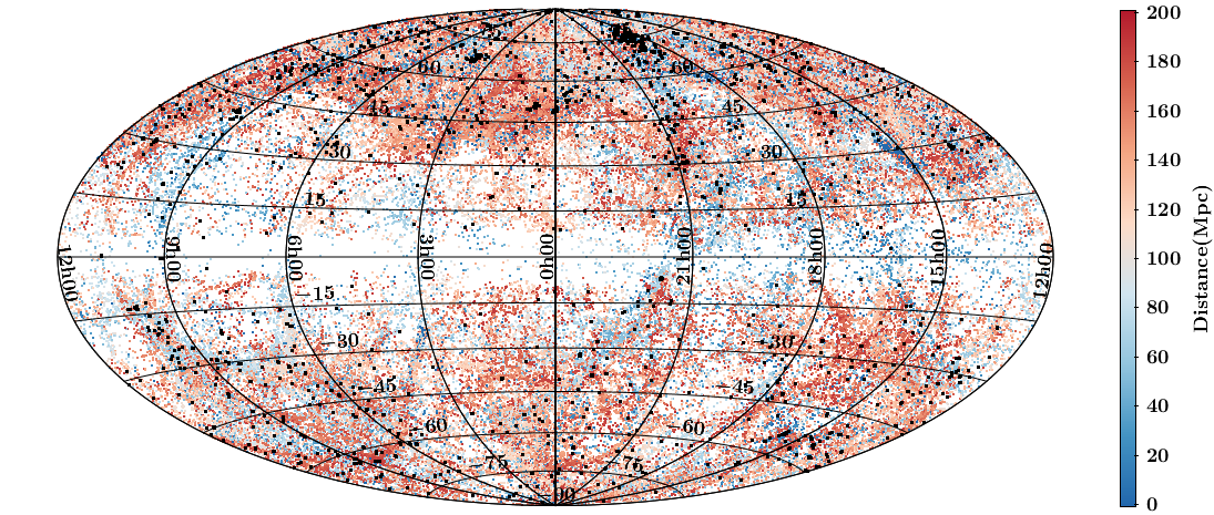
Figure 1: Sky map of the HECATE galaxies in Galactic coordinates with colour denoting their distance. Galaxies included in the CSC 2.0 are shown as black points. Note the sparsity of sources in the plane of the Milky Way (Zone of Avoidance; ZOA) and the increased density in the North and West parts due to the inclusion of SDSS galaxies in the HyperLEDA.

2 The galaxy sample

Table 1: Parameters of the 2218 host galaxies. Only a small portion of this table is shown here, indicative of the various cases (e.g., flags, missing parameters). The full table is available in the online journal.

PGC	ID	$\alpha$	$\delta$	$R_{1}$	$R_{2}$	$\phi$	$T$	$D$	$\log{\rm SFR}$	$\log M_{\star}{}$	$Z$	AGN	$f_{25}$	U	$N_{\rm obs}$	$N_{\rm f/b}$	$N_{\rm ulx}$
(1)	(2)	(3)	(4)	(5)	(6)	(7)	(8)	(9)	(10)	(11)	(12)	(13)	(14)	(15)	(16)	(17)	(18)
2557	NGC0224	10.684684	41.268978	88.91	34.83	35	3.0$\pm$0.4	0.8	-0.33	10.61		Y	0.46		0	0.01	$0.00_{-0.00}^{+1.13}$
16570	NGC1741B	75.398106	-4.263220	0.46	0.23	42	6.8$\pm$3.3	55.7		9.34			1.00	*	2	0.09	$1.91_{-1.13}^{+1.85}$
23324	UGC04305	124.768125	70.721674	3.96	2.79	15	9.9$\pm$0.5	3.4	-2.07	8.77			0.27	*	1	0.00	$1.00_{-0.73}^{+1.49}$
35249	NGC3683	171.882672	56.877021	0.87	0.35	124	4.8$\pm$0.7	33.3	0.94	10.81	8.76	Y	1.00	*	5	0.12	$4.88_{-1.93}^{+2.62}$
38742	NGC4150	182.640252	30.401578	0.99	0.66	148	-2.1$\pm$0.7	13.6	-0.84	9.90		N	1.00	*	2	0.02	$1.98_{-1.14}^{+1.84}$

Columns description: (1) identification number in the HyperLEDA and the HECATE; (2) galaxy name; (3), (4) right ascension and declination (J2000.0) ($\degr$); (5)-(7) the semi-major and -minor axes (′), and the North-to-East position angle (°); (8) morphological code, $T$ (see Table 3); (9) distance (Mpc); (10) decimal logarithm of SFR [$\rm\,M_{\odot}\,yr^{-1}{}$]; (11) decimal logarithm of $M_{\star}$ [$\rm\,M_{\odot}$]; (12) metallicity ($12+\log\left(O/H\right)$); (13) the galaxy hosts an AGN; (14) fraction of $D_{25}$ covered by the CSC 2.0 stacks; (15) * if the galaxy is used in the analysis in this paper (see §3.2); (16) number of observed sources with $L_{X}{>}10^{39}\,\text{erg}\,\text{s}^{-1}{}$, excluding nuclear sources if the host is classified as AGN (see §3.7); (17) number of expected foreground/background source contamination in the ULX regime; (18) number of ULXs by subtracting interlopers. Columns (1)-(13) are taken from the HECATE, while the rest are described in §3.

We use the Heraklion Extragalactic Catalogue (HECATE), a compilation of all galaxies within $200\,\text{Mpc}$, from the HyperLEDA (Makarov et al., 2014), arguably the most complete compilation of galaxies with homogenised parameters. The HECATE adopts positions, sizes, morphological classifications, and redshifts from the HyperLEDA. These are complemented with size and redshift information from other catalogues when not available in the HyperLEDA. It also provides robust estimates of distances, along with SFRs, stellar masses, metallicities and nuclear activity classifications. In the following paragraphs we provide a brief summary of the relevant properties of the catalogue. A detailed description of the catalogue and the data it contains is presented in Kovlakas et al. (in prep).

The HECATE is based on all HyperLEDA galaxies (object type ‘G’) with Virgo-infall corrected radial velocities less than $14000\rm\,km\,s^{-1}$ (corresponding to distances ${\lesssim}200\,\text{Mpc}$ and redshifts ${\lesssim}0.047$). When redshift and size information (semi-major/minor axes and position angles) are not directly available in the HyperLEDA, they are obtained from other databases or catalogues (e.g., NED, SDSS, 2MASS). Figure 1 shows the position of the galaxies in the HECATE in Galactic coordinates.

The HECATE provides redshift-independent distances (e.g., based on the Cepheids, RR Lyrae, Tully-Fisher, surface-brightness fluctuations, tip of the red-giant branch methods) for ${\sim}10\%$ of the galaxies obtained from the NED-D (Steer et al., 2017). When only one distance measurement is available, it is adopted as is. In the case of multiple distance measurements, a statistical estimate is made using a weighted Gaussian Mixture model, with weights that penalise uncertain or old measurements. Subsequently, these distances along with the radial velocities for the same galaxies are used to train a Kernel Regression model which is the used to predict the radial-velocity based distance (and its uncertainty based on the intrinsic scatter) for all the other objects. More details on the method for calculating the galaxy distances are given in Kovlakas et al. (in prep).

The HECATE provides SFR estimates for galaxies with reliable mid- and far-infrared photometric measurements from the IRAS and the WISE. Depending on the availability and quality of photometry, three different SFR indicators were computed based on IRAS photometry: (i) total-infrared (TIR; 24, 60 and $100\mu$ calibrations of Dale & Helou 2002 and Kennicutt & Evans 2012), (ii) far-infrared (FIR; 60 and $100\mu$ calibrations of Helou & Walker 1988 and Kennicutt 1998), and (iii) $60\mu$ (calibrations of Rowan-Robinson 1999). Additionally, WISE photometry, obtained from the forced photometry catalogue of Lang et al. (2016) for galaxies in the SDSS footprint, is used to provide $12\mu$ and $22\mu$-based SFR estimates (calibrations of Cluver et al. 2017). An ‘adopted’ SFR for each galaxy is obtained by homogenising the SFR indicators (using the TIR-based one as reference) and selecting for each galaxy the first available SFR estimate in the following order of preference: TIR, FIR, $60\mu$, $12\mu$, $22\mu$. It should be noted that H$\alpha$ SFR indicators are more appropriate than infrared (IR) indicators for studying the connection of ULXs with young stellar populations, since the latter probe star formation at scales (${\sim}100\,\rm Myr$), longer than the life-time of HMXBs (cf. Kouroumpatzakis et al. 2020). However, IR photometry is readily available for a significant fraction of our sample, and it is generally well correlated with H$\alpha$.

The integrated 2MASS $K$-band photometry and SDSS $g{-}r$ colour, were used to estimate the stellar masses of the galaxies, using the mass-to-light ratio calibrations of Bell et al. (2003). For galaxies without SDSS photometry, the HECATE assumes the mean mass-to-light ratio of the galaxies with SDSS data.

In addition, the HECATE includes gas-phase metallicities based on SDSS spectroscopic data from the MPA-JHU catalogue (Kauffmann et al., 2003; Brinchmann et al., 2004; Tremonti et al., 2004), using the O iii-N ii calibration in Pettini & Pagel 2004. Based on the star-light subtracted SDSS spectra, the HECATE identifies AGN on the basis of their location in optical emission-line ratio diagnostic diagram, using the multi-dimensional classification scheme of Stampoulis et al. (2019).

The Third Reference Catalogue of Bright Galaxies (RC3; de Vaucouleurs 1991) has been the reference galaxy sample for several studies of ULXs (e.g. Swartz et al., 2011; Wang et al., 2016; Earnshaw et al., 2019). While it provides a wide range of information (positions, diameters, morphological types, photometry, and radial velocities), its small size (23022 galaxies) has been superseded by larger and more complete samples of galaxies. The HyperLEDA, and subsequently the HECATE, provide a ${\sim}10$ times improvement in the sample size within our volume of interest ($D{<}200\,\,\text{Mpc}{}$). Therefore, the HECATE, provides a much more complete census of the galaxy populations in the local Universe, supplemented by a wealth of additional information described in the previous paragraphs. This makes it more appropriate for the exploration of the multi-wavelength properties of galaxies based on serendipitous surveys.

3 The X-ray sample

To identify ULX candidates, we use the CSC 2.0, which is a publicly available catalogue of all the sources detected in Chandra observations performed up to the end of 2014. It contains 317167 X-ray sources, an improvement of more than a factor of $3$ compared to the previous version (version 1.1; Evans et al., 2010).

3.1 Selection of sources

An X-ray source is associated with a HECATE galaxy if it is located within its $D_{25}$ region. The positional uncertainties of the sources are not considered, since they are negligible with respect to the dimensions of the galaxies: 95% (98%) of the sources have uncertainties less than the 1% (10%) of the semi-major axes of their host galaxies. The few, galaxies without size information in the HECATE (${\sim}2\%$ of the full sample) are excluded from the cross-matching.

Out of the 317167 sources in the CSC 2.0, we associate 23043 sources to 2218 galaxies within a distance of 200 Mpc. The host galaxies are shown by black points in Figure 1. The parameters of the host galaxies are listed in Table 1 (columns (1)-(13)), while the properties of the selected X-ray sources are given in Table 2.

Table 2: Properties of the 23043 X-ray sources. Only a small portion of this table is shown here, indicative of the various cases (e.g., flags, missing parameters). The full table is available in the online journal.

PGC	ID	$\alpha$	$\delta$	$\log f$	$\log f_{\rm lo}$	$\log f_{\rm hi}$	p	u	n	$c$	$\log L_{\rm X}$	$\log L_{\rm X,lo}$	$\log L_{\rm X,hi}$
(1)	(2)	(3)	(4)	(5)	(6)	(7)	(8)	(9)	(10)	(11)	(12)	(13)	(14)
101	2CXO J000120.2+130641	0.33422	13.11141	-14.37	-14.54	-14.25				0.14	39.44	39.28	39.56
1305	2CXO J002012.6+591501	5.05281	59.25038	-13.36	-13.40	-13.32		*		0.97	36.47	36.42	36.50
2789	2CXO J004732.9-251748	11.88735	-25.29692	-12.15	-12.16	-12.15	*			0.17	39.02	39.01	39.03
12997	2CXO J032953.1-523054	52.47155	-52.51524	-13.87	-13.97	-13.80			*	0.02	40.60	40.51	40.68
42038	2CXO J123622.9+255844	189.09568	25.97891			-15.05		*		0.09			37.24

Columns description: (1) identification number of host galaxy in the HyperLEDA and the HECATE; (2) name of master source in the CSC 2.0; (3), (4) right ascension and declination (J2000.0) ($\degr$); (5)-(7) decimal logarithm of flux (‘flux_aper90_b’) and its 68% confidence interval [$\rm\,erg\,s^{-1}\,cm^{-2}$]; (8) * if pileup source (lower limit on flux and luminosity); (9) * if ‘unreliable’ source (see §3.1); (10) * if nuclear source; (11) galactocentric scale parameter; (12-14) decimal logarithm of X-ray luminosity and its 68% confidence interval [$\,\text{erg}\,\text{s}^{-1}{}$]. The data in columns (2)-(8) are taken directly from the CSC 2.0, while those in columns (9)-(14) are described in §3.

We characterise sources as ‘reliable’ or ‘unreliable’ (column (9) in Table 2) based on their attributes in the CSC 2.0. A source is marked as ‘unreliable’ if any of the following conditions are met:

1. the flux is zero (i.e., upper limit) or no confidence interval is provided,

2. the ‘dither_warning_flag’ is on: indicating that the highest peak of the power spectrum of the source occurs at the dither frequency (or its beat frequency) in all observations,

3. the ‘streak_src_flag’ is on: the source is found on an ACIS readout streak in all observations,

4. the ‘sat_src_flag’ is on: saturated in all observations.

We find 3783 (16.4%) ‘unreliable’ sources, out of which, 1040 (4.5%) are characterised as such because of a flag, 1952 (8.5%) have zero flux, and 791 (3.4%) have missing confidence intervals. The remaining 19260 sources (83.6%) are characterised as ‘reliable’. In the following analysis we consider only the ‘reliable’ sources. We note that the majority of the more luminous sources in our sample ($L_{\rm X}{\gtrsim}10^{41.5}\,\text{erg}\,\text{s}^{-1}{}$) are flagged as ‘unreliable’ (see §4.1), since they are more likely to be saturated.

3.2 Chandra field-of-view coverage

The Chandra observations from which the X-ray sources in the CSC 2.0 are observed, typically target individual galaxies. The field of view is usually centred on the galaxy and covers fully its $D_{25}$ region. However, there are cases of large nearby galaxies that are partially covered, as well as, observations that target off-centre regions.

In order to measure the coverage of each galaxy by Chandra, we compute the fraction, $f_{25}$, of the $D_{25}$ region in the union of the stack-field-of-view of all the stacks contributing in the CSC 2.0 (column (11) in Table 1). We consider galaxies with $f_{25}>0.7$ as sufficiently covered. After visually inspecting multi-wavelength images of the galaxies without full coverage, we find that the missing area generally leaves a negligible fraction of the total SFR and $M_{\star}$ unaccounted for.

We find 34 galaxies (${<}2\%$) with coverage less than 70%. Some galaxies may have poor coverage because of observations performed in sub-array mode (e.g., those focusing on known ULXs.) Excluding these galaxies would bias our demographics; on the other hand, ULXs that are located in the unobserved area of the galaxies would also provide an incomplete picture of ULX populations. For this reason, we manually inspect for the presence of bright sources in XMM-Newton observations with wider field-of-view. Such observations are available for 16 objects, for which we find no other bright ($L_{\rm X}{>}10^{39}\,\text{erg}\,\text{s}^{-1}{}$) sources in their $D_{25}$ regions. Therefore, we include them in the following analysis since their ULX population is complete in our Chandra-based sample. The remaining 18 galaxies are excluded from the subsequent analysis (most of which are known to not host ULXs, e.g., SMC), but not from the provided catalogues.

3.3 Survey coverage and representativeness

3.3.1 Source confusion

At large distances, source confusion severely limits X-ray binary population studies. This effect is more prominent in studies of young stellar populations (such as ULXs; e.g., Anastasopoulou et al. 2016; Basu-Zych et al. 2016) due to the clumpy nature of star-forming regions (e.g., Elmegreen & Falgarone, 1996; Sun et al., 2018). Specifically, at $D{>}40\,\text{Mpc}{}$, the half-arcsecond beam of Chandra is comparable to the angular sizes of typical star-forming regions (${\lesssim}0.5\rm\,kpc$; see discussion in Anastasopoulou et al. 2016). For this reason we restrict our analysis to the 644 galaxies in the host galaxy sample that are closer than $40\,\text{Mpc}$. This allows for direct comparisons with the works of Grimm et al. (2003) and Mineo et al. (2012) which adopt similar distance limits.

3.3.2 Observer bias

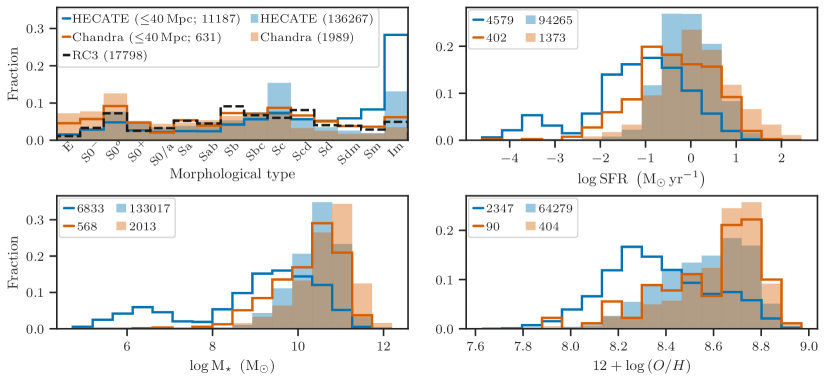
Figure 2: Distribution of morphological types (upper left), SFRs (upper right), $M_{\star}$ (lower left) and gas-phase metallicities (lower right) for the total volume of the HECATE (light blue bins) and the $D{<}40\,\text{Mpc}$ subset (blue steps), as well as, the HECATE/CSC 2.0 galaxies (light orange bins) and their $D{<}40\,\text{Mpc}$ subset (orange steps). For reference, the distribution of morphological types in the RC3 is shown with dashed black steps in the top left panel. The fractions are computed with respect to the sample size of each subset (shown in the legend).

A limitation of this study is that our ULX sample is not based on a homogeneous, blind survey, but an accumulation of archival data gathered from targeted observations with different selection criteria. The unknown selection function may lead to observer biases, such as an over-representation of starburst galaxies: SFR is connected to the number of ULXs, as well as, other interesting phenomena (e.g. galaxy mergers) which may have been the focus of Chandra observations. To explore any biases or selection effects, Figure 2 shows the distributions of the (a) morphological types (see Table 3 for the morphological classification used in this paper), (b) SFRs, (c) stellar masses, and (d) metallicities for all galaxies with available relevant information in the HECATE. We compare the parent sample with the subset observed by Chandra, in the total volume and the $D{<}40\,\text{Mpc}$ limited sample.

Table 3: Morphological types and corresponding numerical codes (or indices) $T$, as described in the documentation of the Second Reference Catalogue of Bright Galaxies (de Vaucouleurs et al., 1976). Throughout this paper, we consider as early-type galaxies (ETGs) the elliptical ($T{<}{-}3.5$) and lenticular galaxies ($-3.5{<}T{<}{-}0.5$), and as late-type galaxies (LTGs) the rest. The morphological types of the galaxies are taken from the HECATE. Throughout the text, different binnings are described as ranges (e.g., Sdm-Im), and measurements with uncertainty less than $1.0$ in $T$ are considered reliable.

	Elliptical			Lenticular			Early spiral					Late spiral				Irregular (Irr)
Morphological type	cE	E0	E+	S0-	S0o	S0+	S0/a	Sa	Sab	Sb	Sbc	Sc	Scd	Sd	Sdm	Sm	Im
Numerical code, $T$	-6	-5	-4	-3	-2	-1	0	1	2	3	4	5	6	7	8	9	10
	ETGs						LTGs

In terms of morphology, Chandra has observed a slightly larger fraction of ETGs galaxies compared to late-type galaxies, a result of observations of nearby clusters which host larger populations of elliptical galaxies. In the $D{<}40\,\text{Mpc}$ sample, the HECATE includes a large population of irregular galaxies (mostly satellites of Local Group galaxies), though Chandra has observed only a small fraction of them. For comparison with previous works, in the top left panel of Figure 2 we show the distribution of the morphological types in RC3. The distribution is similar to the one of the host galaxy sample with $D{<}40\,\text{Mpc}{}$. We also find that the distributions of $M_{\star}$, SFRs and metallicities of galaxies with Chandra observations in the total volume of the HECATE, are slightly shifted towards larger values than those in the parent sample.

These biases combined with the complex selection function of the HECATE and Chandra samples, do not allow us to calculate the volume density of ULXs. Nonetheless, the fact that the X-ray sample covers a wide range of SFRs, $M_{\star}$ and metallicities characteristic of the local galaxies, allows us to draw representative scaling relations. Figure 3 shows the coverage in the SFR-$M_{\star}$ and sSFR-SFR planes for three different samples: the $D{<}40\,\text{Mpc}$ galaxies in the HECATE, the subset of those that are included in the CSC 2.0, and the subset of the latter hosting ULXs. We note that in this figure we exclude AGN-hosting galaxies to avoid biases in the stellar population parameters (see §3.7). We find that the host sample covers galaxies down to stellar mass of $10^{7.5}\,\rm M_{\odot}$ and SFR of $10^{-2.5}\rm\,M_{\odot}\,yr^{-1}{}$, and is uniform in specific SFR (sSFR).

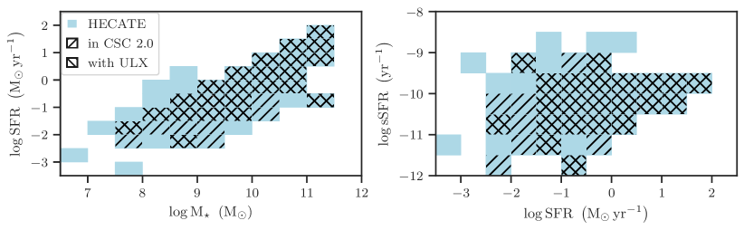
Figure 3: Coverage of the HECATE non-AGN galaxies with $D{<}40\,\text{Mpc}$, in the SFR-$M_{\star}$ (left) and sSFR-SFR (right) planes. Right-angled hatching indicates galaxies covered by the CSC 2.0, while galaxies with left-angled hatching are ULX hosts. It is fairly representative for galaxies of $M_{\star}{>}10^{7.5}\,\rm M_{\odot}$ and ${\rm SFR}{>}10^{-2.5}\,\rm M_{\odot}\,yr^{-1}$ and covers the full sSFR range in this region. ULX hosts (back diagonal hatching) cover the same parameter ranges, however, as expected, more sparsely in the low-SFR regime.

3.4 Galactocentric distances

The shape of the spatial distributions of ULXs in galaxies of different morphological types can provide valuable information regarding their association to the young or old stellar populations, and globular cluster systems. For this reason we calculate the galactocentric distance as the deprojected distance between the source and the centre of the galaxy, assuming the source resides in the disc of the galaxy. In order to normalise the measured galactocentric distance for the size of the galaxy, we derive the galactrocentric scale parameter, $c$ (see Table 2), which we define as the ratio of the deprojected galactocentric distance of the source over the semi-major axis of the latter. A full description of the deprojection method and the calculation of $c$ is presented in Appendix A.

3.5 Source luminosities

In principle, spectral fitting is required for reliable estimates of the source fluxes. Due to the insufficient photon counts for most sources, we use the full-band ($0.5-8.0\rm\,keV$) aperture-corrected net energy flux inferred from the PSF 90% enclosed count fraction aperture as provided by the CSC 2.0 (columns (5)-(7) in Table 2). In the case of sources with multiple observations, their fluxes are estimated from the ‘longest observed segment based on a Bayesian Block analysis of all observations’. We avoid the use of average fluxes (from coadds) since they systematically underestimate the flux of variable sources (e.g., Zezas et al., 2007). Indeed, we find that the above fluxes for our sources are, on average, ${\approx}5\%$ higher than their average⁴ fluxes in the CSC 2.0.

We convert fluxes to luminosities (columns (12)-(14) in Table 2) adopting the distance of the host galaxy in the HECATE (column (6) in Table 1). The luminosities of 49 sources with significant pileup (column (8) in Table 2), are considered as lower limits. However, this does not affect the ULX demographics: their majority (41 sources) are excluded from the ULX demographics as nuclear sources in galaxies hosting an AGN (or without nuclear classification; see §3.7). Three of them are found in poorly-covered galaxies (excluded from our analysis; see §3.2) which are known to not host ULXs (SMC, LMC, Draco Dwarf). The remaining five piled-up sources present luminosities ${>}10^{39}\,\text{erg}\,\text{s}^{-1}{}$ and therefore are bona-fide ULX candidates, but their small number does not bias the luminosity distributions presented in this paper, while they are fully accounted for in the demographics.

3.6 Foreground/background contamination

The main source of contamination in large-area surveys are background (e.g. AGN) and foreground (e.g. stars) objects. Even through we cannot classify individual X-ray sources in our sample as ULXs, AGN, or other classes, using statistical techniques we can remove the effects of these contaminants from our analysis. As a first step we quantify the expected number of foreground/background (f/b) sources in the CSC 2.0 footprint for each galaxy.

There are two commonly used methods to estimate the surface density of interlopers, based on: (i) blank fields around the target galaxies (e.g., Wang et al., 2016), and (ii) the average $\log{N}$-$\log{S}$ distribution from wide-area and deep surveys (e.g., Swartz et al., 2011). Since the former method requires around each object the presence of blank areas wide enough to allow the reliable estimation of the interlopers, which is not always the case, we choose the $\log N$-$\log S$ method. We estimate the number of interlopers in the ULX regime in a given galaxy, by rescaling the $\log N$-$\log S$ for the Chandra-covered fraction of the $D_{25}$ area of the galaxy, and integrating it down to the flux corresponding to $10^{39}\,\text{erg}\,\text{s}^{-1}{}$ for its distance. We use the $\log N$-$\log S$ from the Chandra Multiwavelength Project (ChaMP; Kim et al., 2007, model ‘Bc’ in their table 3). We account for uncertainties in the galaxy distances and the ChaMP $\log{N}$-$\log{S}$ parameters by Monte Carlo sampling from the corresponding Gaussian error distributions, assuming parameter independence. The expected f/b contamination in each galaxy is given in column (14) of Table 1.

The second step is to estimate the number of bona-fide ULXs in each galaxy given the number of observed sources and the previously calculated background contamination. We model the total number of sources as a mix of ULXs and interlopers, assuming both populations are Poisson distributed. We determine the posterior distribution of the number of ULXs, following the Bayesian method described in Park et al. (2006) with the modification that the background ‘counts’ in our case are not directly measured but estimated from the $\log{N}$-$\log{S}$. Specifically,

$$\begin{split}N_{\rm obs}&=N_{\rm ulx}+N_{\rm f/b}\\ N_{\rm ulx}&\sim{\rm Pois}(\lambda)\\ N_{\rm f/b}&\sim{\rm Pois}(\beta),\end{split}$$

where $N_{\rm obs}$ is the observed number of sources in each galaxy: the sum of $N_{\rm ulx}$ ULXs and $N_{\rm f/b}$ interlopers. The latter follow Poisson distributions of means $\lambda$ and $\beta$, respectively, which are independent because the ULX sources in the target galaxy and the foreground/background sources are disconnected populations:

$$N_{\rm obs}\sim{\rm Pois}(\lambda+\beta)\quad\text{and}\quad P(\lambda,\beta)=P(\lambda)P(\beta).$$

To estimate the expected number of ULXs for each galaxy we compute the posterior distribution, marginalised over $\beta$:

$$P(\lambda|N_{\rm obs})=\int\limits_{0}^{\infty}P(\lambda,\beta|N_{\rm obs}){\,\rm d}\beta,$$

where

$$P(\lambda,\beta|N_{\rm obs})\propto P(N_{\rm obs}|\lambda,\beta)P(\lambda,\beta)=P(N_{\rm obs}|\lambda,\beta)P(\lambda)P(\beta).$$

In order to account for uncertainties in the parameters of the $\log N$-$\log S$ distribution, the number of interlopers $\beta$ is not fixed, but allowed to vary. Specifically, the prior for $\beta$ is obtained by evaluating the $\log N$-$\log S$ for varying values of its best-fitting parameters. This is performed by taking $M{=}10000$ samples of the parameters from the corresponding Gaussian distributions (best-fiting values as means, and uncertainties as standard deviations), ultimately giving $M$ samples, $\beta_{i}$, which represent the distribution of $\beta$. By design, the samples $\beta_{i}$ have equal probability to be sampled, $P(\beta_{i}){\propto}1$. For a uniform prior for $\lambda$, $P(\lambda){\propto}1$, and sufficiently large $M$, the marginalised posterior takes the form

$$P(\lambda|N_{\rm obs})=P(N_{\rm obs}|\lambda,\beta)P(\beta)P(\lambda)\propto\sum\limits_{i=1}^{M}P(N_{\rm obs}|\lambda,\beta_{i}),$$

where

$$P(N_{\rm obs}|\lambda,\beta_{i})\propto\left(\lambda+\beta_{i}\right)^{N_{\rm obs}}e^{-\lambda-\beta_{i}},\quad\lambda\geq 0.$$

From the resulting posterior distribution for each galaxy, we compute the mode and the highest posterior density interval corresponding to $68\%$ probability. The observed number of sources ($N_{\rm obs}$), and the estimate on the number of ULXs ($N_{\rm ulx}$) for each galaxy in our sample are listed in Table 1 (columns (13) and (15) respectively).

To evaluate the accuracy of this method, we compare against the previously published ULX catalogue of Wang et al. (2016) which uses the ‘blank fields’ approach. We perform this comparison for the 343 galaxies in the sample of Wang et al. (2016) that are common with our sample. We adopt the same luminosity cut ($2{\times}10^{39}\,{\rm erg\,s^{-1}}$), distance and area on the sky for each galaxy as Wang et al. (2016). We exclude four very local galaxies from this comparison because the $2\times 10^{39}\,\text{erg}\,\text{s}^{-1}$ limit corresponds to brighter fluxes than those used to derive the ChaMP $\log{N}$-$\log{S}$. The results of the comparison of the two methods are shown in Figure 4. We find that both approaches agree in the total number of interlopers: $33.1{\pm}0.1$ (‘blank fields’) and $36.4{\pm}0.3$ ($\log N$-$\log S$) interlopers in the galaxies used for this comparison. The results on individual galaxies are in good agreement for the majority of them: $3\sigma$ consistency for 90% of the objects. A possible explanation for the disagreement of the two methods for the remaining 10% of the galaxies is the fact that the ‘blank fields’ method is based on observations of the individual galaxies, and therefore able to account for the cosmic variance at their location. However, this estimate suffers from incompleteness, due to the degradation of the PSF at the larger off-axis angles from which the background sources are sampled (note that the $\log N$-$\log S$ estimate is on average 10% higher than the ‘blank fields’ estimate).

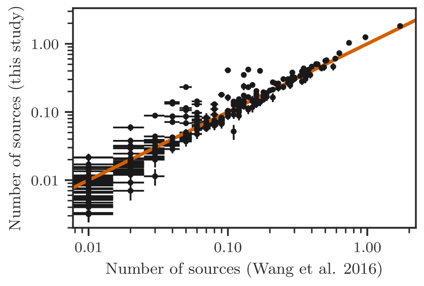
Figure 4: Comparison between the expected foreground/background number of sources from ‘blank fields’ approach (Wang et al., 2016), and $\log{N}$-$\log{S}$ (this study), down to a luminosity limit of $2{\times}10^{39}\,\text{erg}\,\text{s}^{-1}$. The orange line indicates the 1:1 relation. The $x$-error bars are equal to $0.005$ counts because of the $0.01$ precision of the reported values from Wang et al. (2016) and the $y$-error bars reflect the uncertainty from the $\log{N}$-$\log{S}$ parameters.

3.7 AGN in the host galaxies

The presence of AGN in the host galaxies can affect our investigation of ULX populations in two ways:

1. While AGN typically have $L_{\rm X}{>}10^{42}\,\,\text{erg}\,\text{s}^{-1}{}$ (e.g., Brandt & Alexander, 2015), they may exhibit X-ray luminosities as low as $10^{39}$-$10^{40}\,\text{erg}\,\text{s}^{-1}{}$ (e.g., Ho et al., 2001; Ghosh et al., 2008; Eracleous et al., 2002), and therefore may contaminate the sample of luminous X-ray binaries. We account for this by excluding from the demographics (but not the provided catalogues), the nuclear sources in any galaxies classified as AGN, as well as, in galaxies for which we do not have any information on their nuclear activity. We consider sources as nuclear if they are located in the central $3\,\text{arcsec}$ region. These sources are indicated in column (10) in Table 2. Note that this practice unavoidably removes circum-nuclear XRBs (e.g., Wang et al., 2016; Gong et al., 2016).

2. The IR component of the AGN emission will overestimate the inferred SFR and $M_{\star}$ of the host galaxy, and it will bias the measured metallicity (e.g., Mullaney et al., 2011; Delvecchio et al., 2020). While the magnitude of this effect can be small in the case of low-luminosity AGN, we take the conservative measure of excluding any AGN hosts (or galaxies with no nuclear activity information) from our scaling relations. However, scaling relations considering all galaxies (regardless of nuclear activity), labelled as ‘full’ sample to avoid confusion with the non-AGN sample, are presented in Appendix B and are discussed in the main text when relevant.

To characterise the nuclear activity of the galaxies in our sample, we adopt the classification from the HECATE, which uses two sources of information to identify AGN:

1. Stampoulis et al. (2019) who classified galaxies as AGN based on their location in 4- or 3-dimensional optical emission-line ratio diagnostic diagrams, using spectroscopic data from the MPA-JHU catalogue.

2. She et al. (2017) who investigated galaxies at $D{<}50\,\text{Mpc}{}$, observed by Chandra: the nuclear classifications are either adopted from the literature or determined using archival optical line-ratio spectral data.

A galaxy is classified as AGN host if it is identified as such in either of the two. These studies provide nuclear activity diagnostics for 539 (84%) galaxies out of the 644 host galaxies within $40\,\text{Mpc}$. Note, that the exclusion of AGN in the scaling relations, affects the sample of ETGs more strongly since they have higher chance of having been observed due to their nuclear activity, while spiral and irregular galaxies are usually selected for their XRB populations. This is illustrated in Figure 5 where we plot the fraction of galaxies with AGN as a function of the morphological type, in the parent galaxy sample and the galaxies with Chandra observations.

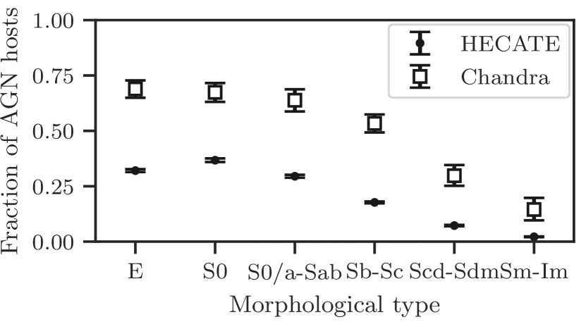
Figure 5: The AGN fraction as a function of the morphological type for the HECATE galaxies (points) and those hosting Chandra sources (squares). The error bars correspond to the 68% CI of the fractions, after accounting for uncertainties on the morphological types, and the Poisson distribution of the number of galaxies.The AGN fraction in Chandra targets is higher than in the general population, especially in elliptical galaxies.

4 Results

In the total volume of the HECATE we find 23043 X-ray sources, out of which 19260 are characterised as ‘reliable’. In the $D{<}40\,\text{Mpc}$ sample which is used for the population statistics presented below, there are 16758 ‘reliable’ X-ray sources, out of which 793 exceed the ULX limit. Of those 793 sources with $L_{\rm X}{>}10^{39}\,\text{erg}\,\text{s}^{-1}{}$ in the $D{<}40\,\text{Mpc}$ volume, 164 (21%) are found close to the centres of galaxies which are classified as AGN hosts, and therefore are not considered as ULX candidates in this study. This leaves a sample of 629 ULX candidates in 309 galaxies, out of which 20% are expected to be foreground/background contaminants (see §4.1).

4.1 Luminosity distribution of X-ray sources

The luminosity distribution of ULXs is crucial for probing the high-end of the luminosity function (LF) of stellar X-ray sources. The calculation of the LF of the XRBs will be presented in a separate paper. Here, we discuss the distribution of X-ray luminosities above the ULX limit.

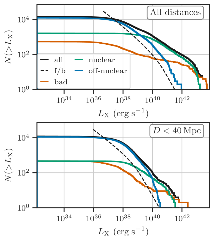
Figure 6: Cumulative number of sources, $N({>}L_{\rm X})$, as a function of X-ray luminosity ($L_{\rm X}$), for various categories: all sources (black), ‘unreliable’ sources (orange), off-nuclear ‘reliable’ sources (blue), nuclear ‘reliable’ sources (green). The expected number of interlopers is shown by the black dashed lines. Top: for all sources in our sample. Bottom: for sources in galaxies with $D{<}40\,\text{Mpc}$.

Figure 6 shows the cumulative distribution of the luminosities of the X-ray sources in our sample in all galaxies (top panel) and in those with $D{<}40\,\text{Mpc}$ (bottom panel). We provide the distribution of all (black), nuclear (green), off-nuclear (blue) and ‘unreliable’ sources (orange; see §2). For reference, we also plot the expected distribution of luminosities of interlopers (f/b; see §3.6). Since we are interested in the contamination of these interlopers within the ULX population, we convert the $\log N$-$\log S$ distribution of the foreground/background sources to the luminosity distribution for the corresponding galaxies using their respective distances. We find that for galaxies within $40\,\text{Mpc}{}$, the background sources (dashed black line) account for ${\sim}20\%$ of all the sources with $L_{\rm X}{>}10^{39}\,\text{erg}\,\text{s}^{-1}$. The contamination dominates the population of the off-nuclear sources at $L_{\rm X}{\gtrsim}10^{40.5}\,\text{erg}\,\text{s}^{-1}$.

The gradual flattening of the luminosity distribution for the total volume (top panel in Figure 6) with decreasing luminosity is a tell-tale sign of incompleteness effects. In the case of the $D{\leq}40\,\text{Mpc}$ distribution (bottom panel), the flattening in the distribution due to incompleteness occurs at ${\sim}~{}3{\times}10^{38}\,\text{erg}\,\text{s}^{-1}$, below the luminosity limit for ULX candidates in this study. In addition, the typical limiting luminosity of sources detected in the galaxies (using the least luminous source) in the total volume of the HECATE, ${\sim}4\times 10^{39}\,\text{erg}\,\text{s}^{-1}$, is above the ULX limit, while in galaxies with $D{<}40\,\text{Mpc}$, it is ${\sim}1.5{\times}10^{38}\,\text{erg}\,\text{s}^{-1}$, well below the luminosity limit for ULX candidates in this study. Therefore, our local sample of ULXs is expected to be complete.

From the top panel of Figure 6 we can see that nuclear sources outnumber the off-nuclear sources above $2{\times}10^{39}\,\text{erg}\,\text{s}^{-1}$ in the full-volume sample. This is partly the result of the larger distances of galaxies in the full volume survey leading to more significant source confusion: in the dense stellar environment of the galactic cores the sources are blended, ultimately flattening the luminosity distribution. Instead, at the $D{<}40\,\text{Mpc}$ sample, the source confusion is significantly reduced: the nuclear sources dominate the sample at a higher luminosity ${\sim}10^{40}\,\text{erg}\,\text{s}^{-1}$, as it is expected by the population of AGN.

4.2 Morphology of ULX hosts and spatial distribution of sources

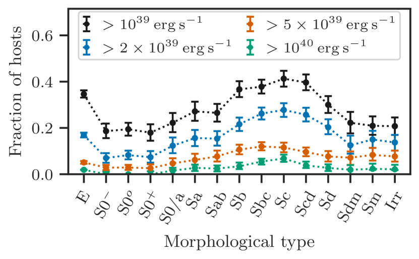
Figure 7: Fraction of galaxies in the HECATE/CSC 2.0 hosting at least one off-nuclear source above the ULX limit (black) as a function of the morphological type. Different colours indicate different limits: $2{\times}10^{39}\,\text{erg}\,\text{s}^{-1}$ (blue), $5{\times}10^{39}\,\text{erg}\,\text{s}^{-1}$ (orange) and $10^{40}\,\text{erg}\,\text{s}^{-1}$ (green). The error bars indicate the 68% CIs, after accounting for the uncertainties on the morphological classifications.

Early ULX population studies, showed that ULXs preferentially occur in late-type galaxies, with only a small fraction (${\lesssim}20\%$) of elliptical galaxies hosting ULXs (e.g., Swartz et al., 2004; Liu et al., 2006; Swartz et al., 2011), in contrast to the recent studies of Wang et al. (2016) and Earnshaw et al. (2019). To test this, we quantify the probability for a galaxy to host ULXs as a function of its morphological type. Figure 7 shows the fraction of galaxies that host off-nuclear sources above different luminosity thresholds, with respect to all galaxies of the same morphological type with Chandra observations. Sources with luminosities above $10^{39}\,\text{erg}\,\text{s}^{-1}$ appear to be present in about 30% of galaxies in all morphological types. There is slightly higher incidence of ULXs (${\sim}40\%$) in elliptical galaxies and Sb-Scd spiral galaxies, while lenticular and irregular galaxies are less likely to host ULXs (${\sim}20\%$). However, galaxies containing sources with $L_{\rm X}{>}5{\times}10^{39}\,\text{erg}\,\text{s}^{-1}$ are typically of late type.

The spatial distribution of X-ray sources can provide insights into their nature. We would expect the surface density of ULXs to follow the distribution of starlight in the host galaxies. However, Swartz et al. (2011) and Wang et al. (2016) find a flattening of the surface density of ULXs in spiral galaxies at large galactocentric distance, in contrast to their exponential surface brightness profile. In addition, Wang et al. (2016) observe an excess of ULXs at large galactocentric distances in elliptical galaxies.

In order to test these observations, we quantify the spatial distribution of ULXs, by computing their surface density on the basis of their galactocentric distances, $c$, for off-nuclear sources with luminosities above $1$, $2$ and $5{\times}10^{39}\,\text{erg}\,\text{s}^{-1}$. Using the method described in §3.6, we correct for the expected f/b contamination. We perform this exercise for galaxies of different morphological types and distances up to $40\,\text{Mpc}$. The distributions are shown in Figure 8.

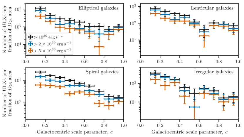
Figure 8: The density of ULXs per fraction of $D_{25}$ area enclosed in annuli with galactocentric distances $c-{\rm d}c$ to $c+{\rm d}c$, as function of $c$, for different luminosity thresholds (colours), and morphological classes of galaxies. The estimates are corrected for f/b contamination. The dips observed in lenticular (at $c{\sim}0.65$) and irregular galaxies (at $c{\sim}0.55$) are statistical fluctuations due to the small numbers of sources; they were found to be sensitive to the binning scheme.

We do not report the number of ULXs at $c{<}0.1$ since it is biased by the exclusion of nuclear sources.

We find that the surface density of ULXs follows the expected exponential trend in spiral galaxies, in contrast to Swartz et al. (2004) and Wang et al. (2016). This disagreement may be caused by foreground/background contamination since it is not accounted for in the spatial distribution analysis of Swartz et al. (2004) and Wang et al. (2016). The number of interlopers scales with area and therefore adds a constant in the surface density profile, effectively flattening the distributions. In our sample, the surface density of ULXs in elliptical galaxies flattens at large galactocentric distances as observed by Wang et al. (2016).

4.3 Rate of ULXs

To quantify the number of ULXs per galaxy as a function of their luminosity for various morphological types, we consider five luminosity thresholds: 1, 2, 3, 5 and 10${\times}10^{39}\,\text{erg}\,\text{s}^{-1}$. We compute the background-corrected number of ULXs above each luminosity threshold, and its 68% confidence intervals, by accumulating the number of observed sources and expected interlopers, and applying the method described in §3.6. The calculation is performed for each morphological class, as well as, the total galaxy sample. Galaxies with uncertain morphological classification are excluded from this analysis (uncertainty in numerical morphological code ${>}1$; see Table 3). By considering non-AGN host galaxies, we also calculate the number of ULXs per total SFR for LTGs, or per total $M_{\star}$ for ETGs. In addition, we also report the number of ULXs per total $M_{\star}$ for all ETGs (‘full’). The results are presented in Table 4.

Table 4: Background-corrected number of ULXs above certain luminosity limits (first line) for different host morphological classes (first column). Square brackets indicate the total number of observed sources followed by the expected number of interlopers. The confidence intervals (68%) account for Poisson uncertainties in both the number of observed sources and the number of interlopers. (A): Number of ULXs divided by the number of host galaxies (second column). The last row (total) refers to all morphological classes. (B): The number of ULXs per $\rm\,M_{\odot}\,yr^{-1}$ of SFR (third column). The last row (LTGs) refers to all late-type galaxies. (C): The number of ULXs per $10^{12}\rm\,M_{\odot}$ stellar mass (third column). The last row (ETGs) refers to all early-type galaxies. (D): As (C), but now considering the full sample of ETGs (not excluding AGN hosts).

We find that the number of ULXs per galaxy for the total population is $0.88{\pm}0.05$ for $L_{\rm X}{>}10^{39}\,\text{erg}\,\text{s}^{-1}$ and $0.20{\pm}{0.02}$ for $L_{\rm X}{>}5{\times}10^{39}\,\text{erg}\,\text{s}^{-1}$. Comparable frequencies are found in early spirals (S0/a-Sb), while in late spirals (Sbc-Sd) they are ${\sim}1.5$ times higher. In elliptical galaxies (E) the ULX frequency per galaxy is slightly lower than that of the total population. Lenticular (S0) galaxies present the lowest frequencies in all luminosity limits, with irregular galaxies following.

The number of ULXs per SFR in irregular galaxies (Sdm-Im) is higher than in spirals, in contrast to their small numbers per galaxy. Early spirals (S0/a-Sb) exhibit the lowest numbers of ULXs per SFR.

Additionally, the ‘full’ sample of ETGs presents lower specific ULX frequencies than the non-AGN sample by a factor of ${\sim}2$. Interestingly, we find that the number of ULXs per $M_{\star}$ is higher in elliptical (E) than in lenticular galaxies (S0) by a factor of ${\sim}2$, a result also observed by Wang et al. (2016). However, this trend disappears when considering the ‘full’ ETG sample: the specific ULX frequencies are consistent within the uncertainties.

Table 5: Fitting results for the scaling factor $a$ (Equation 2) for all LTGs and different morphological classes, and the scaling factor $b$ (Equation 1) for all ETGs, elliptical (E) and lenticular (S0) galaxies. These results are plotted in Figure 9.

Morphology	$N_{\rm gal}$	$N_{\rm src}$	$N_{\rm f/b}$	$a$ ($\rm\,\text{ULXs per }M_{\odot}\,yr^{-1}$)
LTGs	119	123	17.0	$0.51$	${}^{+0.06}_{-0.06}$
S0/a-Sab	11	18	2.9	$0.23$	${}^{+0.07}_{-0.07}$
Sb	12	12	2.2	$0.34$	${}^{+0.14}_{-0.12}$
Sbc	14	26	4.8	$0.44$	${}^{+0.12}_{-0.11}$
Sc	17	19	2.6	$0.51$	${}^{+0.15}_{-0.13}$
Scd	22	23	2.4	$1.54$	${}^{+0.39}_{-0.34}$
Sd-Sdm	23	19	1.7	$2.29$	${}^{+0.67}_{-0.57}$
Sm-Im	20	6	0.5	$2.16$	${}^{+1.19}_{-0.90}$
Morphology	$N_{\rm gal}$	$N_{\rm src}$	$N_{\rm f/b}$	$b$ ($\rm\,\text{ULXs per }10^{12}M_{\odot}$)
ETGs	50	35	8.3	$15.1$	${}^{+3.9}_{-3.6}$
E	22	25	5.5	$21.9$	${}^{+6.4}_{-5.7}$
S0	28	10	2.8	$8.7$	${}^{+4.7}_{-3.8}$
ETGs (full)	195	152	57.6	$6.3$	${}^{+1.0}_{-0.9}$
E (full)	96	104	37.5	$7.5$	${}^{+1.3}_{-1.3}$
S0 (full)	99	47	20.0	$4.8$	${}^{+1.4}_{-1.2}$

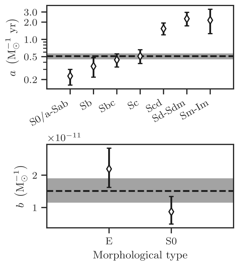
Figure 9: Fitting results for the SFR and $M_{\star}$ scaling factors for different morphological classes. Top: the scaling parameter $a$ (Equation 2) for late-type galaxies (line) and 68% CI (grey band), and for various late-type morphological classes (black error bars). Bottom: same as the top panel, but for the scaling parameter $b$ (Equation 1) for early-type (line and band), elliptical and lenticular galaxies (error bars).

In addition to the above analysis, we perform fits of the number of ULXs against the $M_{\star}$ or SFR of the galaxies. For $N_{\rm obs}$ sources with $L_{\rm X}{>}10^{39}\,\text{erg}\,\text{s}^{-1}{}$ and $N_{\rm f/b}$ expected number of interlopers from the ChaMP $\log N$-$\log S$, we fit the model

$$N_{\rm obs}={\rm Pois}\left(b\times M_{\star}{}+N_{\rm f/b}\right)$$ (1)

for all ETGs with robust morphological classifications (see caption of Table 3), and the subdivisions of elliptical and lenticular galaxies, using the Maximum Likelihood method. In a similar fashion, we fit the model

$$N_{\rm obs}={\rm Pois}\left(a\times\text{SFR}+N_{\rm f/b}\right)$$ (2)

for the LTGs and five sub-populations: S0/a-Sab, Sb, Sbc, Sc, Scd, Sd-Sdm and Sm-Im. The results are listed in Table 5.

For the scaling with $M_{\star}$ in ETGs we find $b{=}15.1^{+3.9}_{-3.6}\rm\,\text{ULXs per }10^{12}M_{\odot}{}$, while in elliptical galaxies it is significantly higher ($21.9^{+6.4}_{-5.7}\rm\,\text{ULXs per }10^{12}M_{\odot}{}$) than in lenticular galaxies ($8.7^{+4.7}_{-3.8}\rm\,\text{ULXs per }10^{12}M_{\odot}{}$). However, in the full ETG sample (i.e. including AGN hosts), the specific ULX frequencies are lower than those in the non-AGN ETGs ($6.3^{+1.0}_{-0.9}\rm\,\text{ULXs per }10^{12}M_{\odot}$). See §5.4 for an explanation of this difference.

In LTGs, we find that the scaling with SFR, $a$, is $0.51{\pm}0.06\rm\,\text{ULXs per }M_{\odot}\,yr^{-1}{}$ (horizontal line in the top panel of Figure 9) and that it monotonically increases with morphological type: from $0.23\rm\,\text{ULXs per }M_{\odot}\,yr^{-1}{}$ (S0/a-Sab) to $2.16\rm\,\text{ULXs per }M_{\odot}\,yr^{-1}{}$ (Sm-Im).

4.4 SFR and stellar mass scaling in late-type galaxies

In order to account for the contribution of ULXs associated with LMXBs (e.g., GRS1915+105-type systems; Greiner et al. 2001), we perform a joint fit of the number of ULXs in LTGs with respect to both their SFR and $M_{\star}$.

The correlation can be visualised by binning the galaxies by SFR and $M_{\star}$ and computing the average number of ULXs per galaxy, for each bin, after removing the f/b contamination (see §3.6). We plot the result in Figure 10, where we see a trend for galaxies with higher SFR and $M_{\star}$ to host larger numbers of ULXs. This trend becomes stronger in regions of high sSFR (indicated by the diagonal lines).

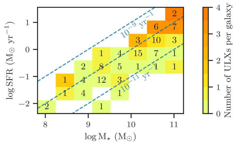
Figure 10: The mean, background-corrected number of ULXs ($N_{\rm ulx}$) per galaxy (color scale) as a function of SFR and $M_{\star}$, in non-AGN LTGs. The diagonal dashed lines correspond to indicative specific SFRs, while the numbers in boxes denote the number of galaxies in each bin. We see a trend for more ULXs in galaxies with high SFR, $M_{\star}$, and sSFR.

While SFR and $M_{\star}$ are known to be correlated in star-forming galaxies (e.g., Rodighiero et al., 2011; Speagle et al., 2014; Maragkoudakis et al., 2017), the SFR is expected to be the primary parameter correlated with the population of ULXs. To study the dependence of $N_{\rm ulx}$ on both parameters, we fit the model

$$N_{\rm obs}\sim{\rm Pois}\left(\alpha\times{\rm SFR}+\beta\times M_{\star}{}+N_{\rm f/b}\right)$$ (3)

where $N_{\rm obs}$ is the total number of observed sources with $L_{\rm X}{>}10^{39}\,\text{erg}\,\text{s}^{-1}$, $\alpha$ and $\beta$ are the scaling factors that will be fitted, and $N_{\rm f/b}$ is the expected number of interlopers (computed in §3.6). The model is applied to all LTGs with robust morphological classifications (see Tables 1, 3) and the two sub-populations of early spirals (S0/a-Sbc), and late spirals / irregular galaxies (Sc-Im). The results are listed in Figure 11, while the joint posterior distributions of $\alpha$ and $\beta$ are shown in Figure 11.

The best-fitting value of the SFR scaling factor for LTGs is $\alpha{=}0.45^{+0.06}_{-0.09}\rm\,\text{ULXs per }M_{\odot}\,yr^{-1}$ while the $M_{\star}$ scaling factor is $\beta{=}3.3^{+3.8}_{-3.2}\rm\,\text{ULXs per }10^{12}M_{\odot}$. For the early-type spirals we find lower $\alpha{=}0.16{\pm}0.08\rm\,\text{ULXs per }M_{\odot}\,yr^{-1}$ and higher $\beta{=}11.2^{+5.2}_{-5.6}\rm\,\text{ULXs per }10^{12}M_{\odot}$, while for the late-type spirals the situation is inverted, i.e. $\alpha{=}0.98^{+0.11}_{-0.20}\rm\,\text{ULXs per }M_{\odot}\,yr^{-1}$ and $\beta$ is consistent with zero (${<}6.6\rm\,\text{ULXs per }10^{12}M_{\odot}{}$).

Table 6: Mode and 68% Highest Posterior (marginalised) Density Intervals of the scaling parameters $\alpha$ and $\beta$ (see Equation 3) for all LTGs and their ‘early’ and ‘late’ subdivisions (see Table 3). For each fit we report the number of galaxies ($N_{\rm gal}$), sources ($N_{\rm src}$) and interlopers ($N_{\rm f/b}$). See below for the joint distributions (Figure 11).

Sample	$N_{\rm gal}$	$N_{\rm src}$	$N_{\rm f/b}$	$\alpha\ \rm(M_{\odot}\,yr^{-1})^{-1}$	$\beta\ (10^{12}\,\rm M_{\odot})^{-1}$
LTGs	106	117	15.8	$0.45^{+0.06}_{-0.09}$	$\phantom{{<}0}3.3^{+3.8}_{-3.2}$
S0/a-Sbc	37	56	9.9	$0.16^{+0.08}_{-0.08}$	$\phantom{<}11.2^{+5.2}_{-5.6}$
Sc-Im	69	61	5.9	$0.98^{+0.11}_{-0.20}$	$\phantom{0}{<}6.6\phantom{{}^{+0.0}_{-0.0}}$

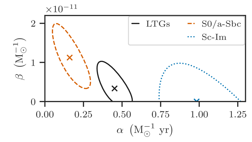
Figure 11: The best-fitting values (X symbols) and, 68% confidence regions (lines) of the scaling parameters $a$ and $b$ of Equation 3 for all LTGs (solid), and the ‘early’ (S0/a-Sbc; orange) and ‘late’ (Sc-Im; blue) spiral galaxies. See Figure 11 for marginalised results.

5 Discussion

5.1 Comparison with other ULX surveys

Our estimate for the scaling of the number of ULXs with SFR ($0.51\pm 0.06\rm\,\text{ULXs per }M_{\odot}\,yr^{-1}{}$; Table 5) is four times lower than that estimated in Swartz et al. (2011; 2$\rm\,\text{ULXs per }M_{\odot}\,yr^{-1}$). This is the result of differences in: (i) the selection of host galaxy sample, and (ii) the method used in the calculation of the X-ray fluxes. When we account for these differences, we find consistent results as discussed in detail in Appendix §C.1.

Furthermore, we would expect our results to agree with those of Wang et al. (2016), since they also use Chandra observations for a similarly large sample of host galaxies (343 galaxies) to study the ULX content in nearby galaxies. However, Wang et al. (2016) consider ULXs at twice our luminosity threshold (i.e., $2\times 10^{39}$) and at larger separations from the galaxy centres ($2{\times}D_{25}$ area instead of $D_{25}$). After accounting for these differences, and a small offset between the computed X-ray fluxes resulting from different methods, we find similar frequency of ULXs in all galaxies, and separately for their different morphological classes (Table 4). See Appendix §C.2 for details of this comparison.

Earnshaw et al. (2019), using a sample of 248 galaxies with sensitivity limit below the ULX limit in their X-ray samples, found that one out of three galaxies host at least one ULX, with spiral galaxies having a slightly higher fraction (${\sim}40\%$) than elliptical galaxies (${\sim}30\%$). This is in agreement with our results (see Figure 7): the fraction of ULX hosts in galaxies of different morphological types is between 20% and 40%, with the peak at Sc galaxies, and a fraction of ${\sim}35\%$ in elliptical galaxies.

5.2 Dependence of number of ULXs on SFR and stellar mass in star-forming galaxies

In §4.3, we find the number of ULXs in LTGs to be $0.51{\pm}0.06$ per $\rm\,M_{\odot}\,yr^{-1}$ (see Table 5), consistent with the expectation from the Mineo et al. (2012) HMXB-LF, of $0.56\rm\,\text{ULXs per }M_{\odot}\,yr^{-1}{}$. We observe a dependence of the scaling factor per SFR (parameter $a$ in Equation 2 and Figure 9) on the morphological type; it monotonically increases from $0.23{\pm}0.07$ to $2.16^{+1.19}_{-0.90}\rm\,\text{ULXs per }M_{\odot}\,yr^{-1}$ from S0/a-Sab to Sm-Im galaxies (Table 5). The higher scaling factor in late spiral and irregular galaxies can be attributed to their lower metallicity with respect to early spiral galaxies (e.g., González Delgado et al., 2015): as discussed in §5.3 low metallicity galaxies show an excess of ULXs. Figure 12 shows the metallicity distribution for different morphological types in the HECATE and our host galaxy sample. We see that the average metallicity quickly drops for galaxies later than Sc, the same galaxies for which the scaling factor (see Table 5) increases from $0.51$ to $1.54\rm\,\text{ULXs per }M_{\odot}\,yr^{-1}{}$. However, these trends do not account for another important factor which cannot be tested in the current sample: late-type galaxies are more prone to short and intense star-formation episodes, which might increase their ULX content significantly (e.g., Wiktorowicz et al., 2017), although the effect of metallicity appears to have a stronger effect in the X-ray output of a galaxy (e.g., Fragos et al., 2013a).

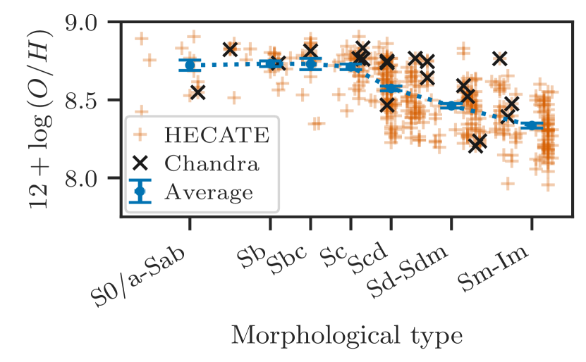
Figure 12: The metallicity, $12+\log\left(O/H\right)$, as a function of the morphological type in the host (‘Chandra’; black ‘x’ markers) and parent (‘HECATE’; orange plus markers) galaxy samples. Note, that only non-AGN galaxies with robust morphological classification and $D{<}40\,\text{Mpc}{}$ are shown. For the morphological types that correspond to the results of the scaling of ULXs with SFR, $a$, in Table 5, we show the mean metallicity and its standard error (blue errorbars). Scd galaxies and later, present the lower metallicities, partly explaining the result that in the same galaxies $a$ is significantly higher than the average in LTGs.

In order to account for the LMXB contribution in LTGs, in §4.3 we computed the scaling parameters $\alpha$ and $\beta$ for the linear relation between number of observed sources with $L_{\rm X}{>}10^{39}\,\text{erg}\,\text{s}^{-1}$ and both SFR and $M_{\star}$ (Equation 3). The value of $\alpha{=}0.45^{+0.06}_{-0.09}\rm\,\text{ULXs per }M_{\odot}\,yr^{-1}{}$ (see Figure 11) for all LTGs is somewhat smaller, but consistent with the value of $a{=}0.51{\pm}0.06\rm\,\text{ULXs per }M_{\odot}\,yr^{-1}{}$ found using the model of Equation 2 where only the SFR scaling is considered (see Table 5). The smaller scaling when accounting for the contribution of the $M_{\star}$ is the result of the small fraction of the ULX population that is associated with the old stellar population (and consequently the $M_{\star}$) in spiral galaxies. The results of the fits for early and late spirals (see Figure 11 and Figure 11) illustrate that the $M_{\star}$ contribution is significant in early spirals (S0/a-Sbc) at the $2\sigma$-level, while it can be neglected in late spirals ($\beta{<}6.6\rm\,\text{ULXs per }10^{12}M_{\odot}{}$ with most probable value 0.0).

Recently, Lehmer et al. (2019) constructed luminosity functions of XRBs as a function of both SFR and $M_{\star}$ to account for the contribution of both LMXBs and HMXBs. Using the best-fitting parameters for their full sample (see table 4 in Lehmer et al. 2019) we integrated the LF above the ULX limit ($10^{39}\,\text{erg}\,\text{s}^{-1}$). We find that they predict $N_{\rm ulx}=a_{\rm L19}{\rm SFR}+b_{\rm L19}M_{\star}{}$, where $\alpha_{\rm L19}=0.62{\pm}0.08\rm\,\text{ULXs per }M_{\odot}\,yr^{-1}{}$ and $\beta_{\rm L19}=18^{+23}_{-11}\rm\,\text{ULXs per }10^{12}M_{\odot}{}$. The scaling with SFR ($\alpha$) is consistent at the $1\sigma$-level with our findings for all LTG galaxies ($0.45^{+0.06}_{-0.09}\rm\,\text{ULXs per }M_{\odot}\,yr^{-1}{}$; see Equation 3). The scaling with $M_{\star}$ ($\beta$) is highly uncertain in the ULX regime, but also consistent at the $1\sigma$-level with the one we find for all LTG galaxies ($3.3^{+3.8}_{-3.2}\rm\,\text{ULXs per }10^{12}M_{\odot}{}$).

Finally, the above results are consistent with the qualitative picture shown in Figure 10; the number of ULXs in LTGs increases with both SFR and $M_{\star}$. Note that the trend of galaxies hosting larger population of ULXs at higher sSFR (see diagonal lines), may have a trivial explanation: ULXs being primarily associated with young stellar populations, are more abundant in galaxies with higher SFR and/or lower mass. However, an age effect may be at the play: starbursts have high sSFR, by definition, and are expected to have high formation rate of BH ULXs, which dominate the population at ${\sim}5\,\rm Myr$ (e.g. Fragos et al., 2013b).

Such an age effect will manifest as an excess of ULXs in high sSFR galaxies compared to the expectation from the average SFR-$M_{\star}$ scaling relation based on all LTGs in our sample. We assess this by defining the excess of ULXs,

$$\text{excess}=\log\frac{N_{\rm obs}}{N_{\rm exp}}$$ (4)

where $N_{\rm obs}$ is the number of ULX candidates, and $N_{\rm exp}$ is the expected number of sources according to the model in Equation 3 and its best-fitting values (Figure 11). In order to explore the possible dependence of the ULX excess on SFR and $M_{\star}$, we plot in Figure 13 the ULX excess of galaxies as a function of their SFR and $M_{\star}$. We do not see a dependence on the sSFR; instead, it is clear that low-mass galaxies present an excess of ULXs, in agreement with Swartz et al. (2008). Since low-mass galaxies tend to present lower metallicities (e.g., Kewley & Ellison, 2008) we interpret this excess as likely being related to the metallicity of their hosts.

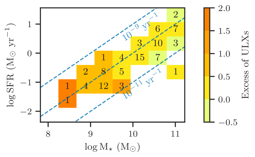
Figure 13: The mean excess of ULXs (colour scale; as expressed in Equation 4) in LTGs as a function of SFR and $M_{\star}$. The diagonal lines correspond to indicative specific SFRs. The numbers in the boxes denote the number of galaxies in each bin. Despite their small numbers, the data show that galaxies with low masses exhibit a clear excess in the number of ULXs over the expectation.

5.3 Excess of ULXs in low-metallicity galaxies

There is a growing observational body of evidence for an excess of ULXs in low-metallicity galaxies (e.g., Soria et al., 2005; Mapelli et al., 2010; Prestwich et al., 2013; Brorby et al., 2014; Tzanavaris et al., 2016). This trend can be interpreted theoretically in the context of the weaker stellar winds in low-metallicity stars. The stars retain higher fraction of their initial mass, and as a consequence, more massive BHs are formed, with smaller orbital separation due to weaker angular momentum losses (e.g., Heger et al. 2003; Belczynski et al. 2010; Marchant et al. 2017). In addition, the tighter orbits result in an increased fraction of HMXBs that enter a Roche-lobe overflow phase, which being a more efficient accretion mechanism than stellar winds, leads to more luminous X-ray sources (Linden et al., 2010).

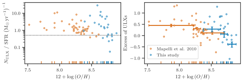
Figure 14: Left panel: the number of ULXs per SFR unit ULXs for LTGs in our sample (blue) with metallicity estimates (blue points), and that of Mapelli et al. (2010) (orange). The metallicities of the galaxies with no sources above the ULX limit, are shown as ticks on the $x$-axis. Low-metallicity galaxies present an excess of ULXs with respect to the average scaling (dotted horizontal line.) Right panel: same as the left panel but now the $y$-axis is the excess of ULXs as defined in Equation 4. We find a significant anti-correlation (Kendall rank correlation coefficient $\tau{=}{-}0.43$ with $p$-value $0.002$). We bin the galaxies to reduce the stochasticity of the ULX excess (see §5.3) and compute the median and 68% CIs of the excess as a function of the metallicity (blue error bars). We repeat the same procedure for the ULX excess in the sample of Mapelli et al. (2010) (orange) which also exhibits significant anti-correlation ( $\tau{=}{-}0.40$ and $p{=}0.001$).

To investigate the correlation of the ULX population with metallicity, we plot in Figure 14 (left) the number of ULXs per SFR as function of the host galaxy metallicity for the 44 galaxies with metallicity measurements in the HECATE (blue circles). We see an excess of ULXs in low metallicities with respect to the average relation shown with the dotted line. In the right panel of Figure 14 we plot the ULX excess (Equation 4) against metallicity. We see that the frequency of ULXs indeed increases with decreasing metallicity (Kendall rank correlation coefficient $\tau{=}-0.43$ with $p$-value of $0.002$). For comparison, we also plot in the same figure the excess of ULXs computed from the sample in Mapelli et al. (2010) (orange circles) using their reported values for (i) the number of ULXs, (ii) the expected background contamination, and (iii) the SFRs of the host galaxies. To reduce the Poisson noise, the galaxies are grouped in metallicity bins (defined to have a similar number of objects in each bin and always more than eight) shown as $x$-axis error bars in Figure 14. The central values and the error bar length in the $y$-axis correspond to the median and the 68% confidence interval of the ULX excess, computed by accounting for Poisson uncertainty of the number of sources and interlopers.

Based on the binned statistics in Figure 14, we find that the galaxies with the lowest metallicities in our sample (corresponding to $0.3$-$0.5\,\rm Z_{\odot}$) host more ULXs per SFR by a factor of ${\sim}2$, in comparison to galaxies of intermediate metallicity ($0.5$-$0.7\,\rm Z_{\odot}$) which present no excess of ULXs. Interestingly, galaxies with near-solar metallicity (${>}0.7\rm\,Z_{\odot}$) present a deficiency of ULXs; they host half of the expected ULX population.

The same trend is observed in the sample of Mapelli et al. (2010). However, there seems to be a small horizontal offset of ${\sim}0.25\rm\,dex$ between our study and that of Mapelli et al. (2010). We attribute this offset to the different metallicity calibrations which can have systematic biases up to $0.7\rm\,dex$ (see fig. 2 in Kewley & Ellison 2008). Using eight common galaxies in our sample and that of Mapelli et al. (2010), we find that the mean offset between the metallicities is $0.28\pm 0.09$.

In conclusion, an excess of ULXs is linked with low-metallicities. This is also in line with our result that the ULX-SFR scaling factor is significantly higher in later-type galaxies, for which the metallicity is lower (see §5.2). This excess has direct implications for the XRB content of the high-redshift Universe. The mean metallicity of galaxies at $z{\sim}2.5$ was only ${\sim}0.1\,\rm Z_{\odot}$ (e.g., Madau & Dickinson, 2014). Indeed, an excess of the integrated X-ray luminosity per unit SFR is seen in observational studies of high-redshift galaxies (e.g., Lehmer et al., 2005, 2016; Basu-Zych et al., 2013a, b, 2016; Brorby et al., 2016; Fornasini et al., 2019, 2020; Svoboda et al., 2019). Our results indicate that this excess is the result of a larger population of luminous X-ray sources per unit SFR in lower metallicities. However, we cannot exclude the possibility that the stellar population age also plays a role on the ULX excess. Since the metallicity and age can vary by region in a galaxy, investigation on sub-galactic scales can help to disentangle their relative effects on the XRB populations (cf. Anastasopoulou et al. 2019; Lehmer et al. 2019; Kouroumpatzakis et al. 2020).

5.4 ULXs and old stellar populations

ULXs in elliptical galaxies (e.g., David et al., 2005) are considered to belong to the high-end of the LMXB-LF (e.g., Swartz et al., 2004; Plotkin et al., 2014). Notably, rejuvenation of stellar populations due to galaxy mergers might also produce additional ULXs (Zezas et al., 2003; Raychaudhury et al., 2008; Kim & Fabbiano, 2010). In addition, it is possible that a small population of ULXs are dynamically formed in GCs (e.g., Maccarone et al., 2007; Dage et al., 2020). Indeed, we find evidence that a small but significant population of ULXs in elliptical galaxies resides at large galactocentric distances (see §4.2), i.e., not following the $M_{\star}$ distributions. Literature review of the hosts of these sources showed evidence for recent merger activity, or large GC populations, indicating that these ULXs could be associated with GCs, given the flatter distributions of GCs and their LMXB populations with respect to the stellar light (e.g., Kim et al., 2006).

In §4.3, based on the fit of the number of ULXs against the $M_{\star}$ of ETGs (see Equation 1), we find $15.1^{+3.9}_{-3.6}\rm\,\text{ULXs per }10^{12}M_{\odot}{}$ in the non-AGN sample. However, it is higher by a factor of $2$-$3$ than the expectation from the LMXB-LF of Zhang et al. (2012) ($5\pm 2\rm\,\text{ULXs per }10^{12}M_{\odot}$), and the specific ULX frequency in Plotkin et al. (2014) ($6.2\pm 1.3\rm\,\text{ULXs per }10^{12}M_{\odot}$) and Walton et al. (2011) (${\sim}7\rm\,\text{ULXs per }10^{12}M_{\odot}$). While these studies address possible contamination from AGN in their X-ray source samples, they still consider (except for Zhang et al. 2012) the total $K$-band luminosity of the galaxies as a tracer of the $M_{\star}$ even if the galaxy hosts an AGN. The contamination by the AGN would lead to an overestimation of the $M_{\star}$, and consequently an underestimation of the specific ULX frequency. To quantify this effect, in Appendix B we compute the specific ULX frequency in the full sample (including galaxies hosting AGN, but still excluding their nuclear sources). We find $6.3^{+1.0}_{-0.9}\rm\,\text{ULXs per }10^{12}M_{\odot}{}$ in good agreement with the literature estimates.

Why do non-AGN ETGs exhibit higher specific ULX frequency than the ‘full’ ETG sample? As we show in Appendix B the presence of an AGN does not significantly affect the observed $K$-band luminosity and therefore the measured $M_{\star}$. The AGN contribution is ${<}10\%$ of the total $K$-band luminosity (Bonfini et al. 2020, submitted). However, the full sample extends to much larger masses than the non-AGN ETG sample. Consequently, the difference in the specific ULX frequency between the full and non-AGN sample could be explained by a non-linear dependence of the number of ULXs on the $M_{\star}$.

In order to quantify the dependence of the specific ULX frequency on the $M_{\star}$, we compute the scaling factor $b$ in our ETG sample, over three $M_{\star}$ bins ($10^{9.5}-10^{10.0}$; $10^{10.0}-10^{10.5}$; $10^{10.5}-10^{11.0}\,\rm M_{\odot}$), separately for AGN and non-AGN galaxies. This is shown in Figure 15. The results for the AGN and non-AGN samples agree within the errors, as expected based on the previous assessment that the AGN do not lead to significant overestimation of the $M_{\star}$ (see Appendix B). They also agree with the scalings reported in Zhang et al. (2012) and Plotkin et al. (2014) for the corresponding $M_{\star}$ bins (also plotted in Figure 15). Interestingly, however, we find that $b$ depends strongly on the $M_{\star}$ of the host galaxy. This dependence explains the lower specific ULX frequency found in the ‘full’ ETG sample which is biased towards more massive galaxies than in the case of non-AGN ETG sample.

The dependence of the specific ULX frequency on the $M_{\star}$ could be caused by star-formation history (SFH) differences in ETGs (McDermid et al., 2015). Simulations indicate that ULXs with neutron-star accretors and red giant or Hertzsprung-gap donors can appear several hundreds of Myrs after a star-formation episode (Wiktorowicz et al., 2017), and therefore their frequency in early-type galaxies is expected to be strongly dependent on the SFHs. Calculated specific ULX frequencies (circles in Figure 15) using the Wiktorowicz et al. (2017) simulation and the McDermid et al. (2015) average SFHs for the same stellar mass ranges (see §5.5), are in excellent agreement with the observed specific ULX frequencies in our sample.

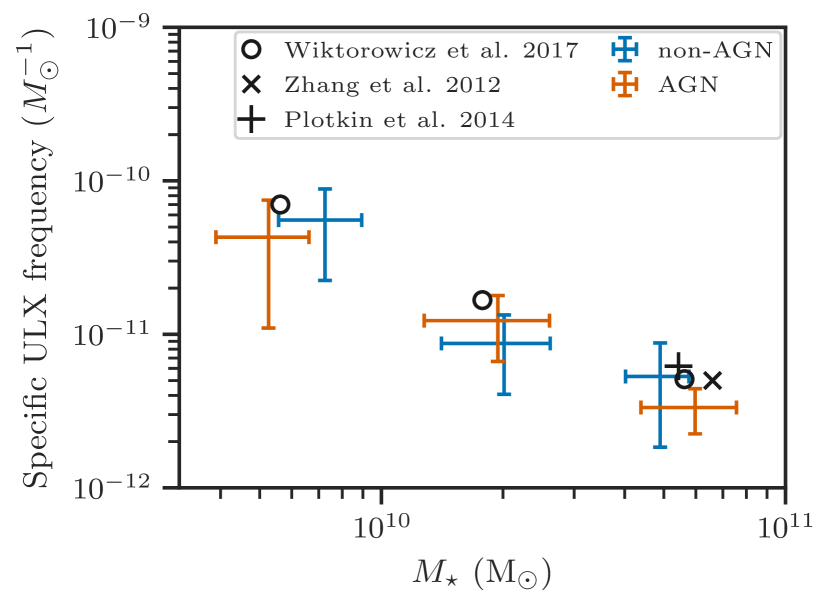
Figure 15: The specific ULX frequency for ETGs in our sample with stellar masses in the ranges $10^{9.5}$-$10^{10}$, $10^{10}$-$10^{10.5}$ and $10^{10.5}$-$10^{11}\,\rm M_{\odot}$, for AGN (orange error bars) and non-AGN galaxies (blue error bars). The cross and plus markers indicate the specific ULX frequency and the mean stellar mass of the samples in Zhang et al. (2012) and Plotkin et al. (2014). The circles indicate the computed values by convolving the binary population synthesis results of Wiktorowicz et al. (2017) with average SFH of ETGs in McDermid et al. (2015). Note that the $x$-axis error-bars do not indicate bin widths, but the standard deviation of the stellar masses of the galaxies contributing in each bin, to give a sense of the stellar mass distribution in each bin.

Therefore, comparisons of ULX rates in ETGs should account for the mass range covered in each sample and the corresponding bias due to different SFHs. In this respect, we attribute differences between our estimates of the specific ULX frequency and those of previous studies to the different $M_{\star}$ ranges in the samples. Note, however, that the specific ULX frequency was found to be constant in elliptical galaxies in Walton et al. (2011), albeit with a relatively small sample of 22 galaxies.

Furthermore, in §4.3 we find that lenticular galaxies in our sample host 2-3 times fewer ULXs than elliptical galaxies, by a factor of $2$-$3$, even when normalising by the $M_{\star}$. This result is in agreement with the findings of Wang et al. (2016). However, we noticed that this difference disappears when considering the ‘full’ sample. Given the dependence of the specific ULX frequency on the $M_{\star}$ shown in Figure 15, it is possible that this discrepancy stems from the different $M_{\star}$ regimes of the corresponding samples. Indeed, we find that the interquartile range (middle 50%) of the stellar masses in the ‘full’ sample lies in the $1.6{\times}10^{10}\rm\,M_{\odot}{}$-$10^{11}\rm\,M_{\odot}{}$ range, for both elliptical and lenticular galaxies, while in the case of the non-AGN sample, lenticular galaxies present higher masses, $1.4$-$4{\times}10^{10}\rm\,M_{\odot}{}$, compared to that of the elliptical galaxies, $0.5$-$3.5{\times}10^{10}\rm\,M_{\odot}{}$.

5.5 Comparison with models

Comparison of binary population synthesis models and demographic studies of ULXs provide tests for models of the formation and evolution of X-ray binaries with extreme mass transfer rates.

We compare our findings with the results in Wiktorowicz et al. (2017), who computed the observed number of ULXs as a function of time for three different metallicities (0.01, 0.1 and 1 $Z_{\odot}$). Since the SFR indicators used in our study are based on the IR emission which is sensitive to stellar populations of ages up to ${\sim}100\rm\,Myr$ (Kennicutt & Evans, 2012), we compare our results with the number of ULXs reported in Wiktorowicz et al. (2017) observed after $100\,\rm Myr$ for a starburst scenario for $6\times 10^{10}\,\rm M_{\odot}$ of stars formed with $100\,\rm Myr$ duration. They report $4\times 10^{2}$ ULXs which corresponds to a formation rate of $0.67\rm\,\text{ULXs per }M_{\odot}\,yr^{-1}$. This value is close to our results for all LTGs ($0.51{\pm}0.06\rm\,\text{ULXs per }M_{\odot}\,yr^{-1}{}$; see Table 5).

To study the effect of metallicity, we also consider the $0.1\,Z_{\odot}$ simulation from Wiktorowicz et al. (2017). The resulting formation rate is $12\rm\,\text{ULXs per }M_{\odot}\,yr^{-1}{}$, about 18 times stronger than that in the case of $Z{=}Z_{\odot}$. As shown in Figure 14, our sample at such low metallicities is insufficient to estimate the excess of ULXs. However, we find an excess of ${\sim}0.7\rm\,dex$ in the ULX rate for ${\sim}0.3\rm\,dex$ lower metallicities in comparison to the bulk of the galaxies (which are predominantly solar metallicity galaxies). This translates to a factor of ${\sim}5$ more ULXs at $Z{=}0.3Z_{\odot}$ which is between the expectations from the models of Wiktorowicz et al. (2017) for $Z{=}0.1\,Z_{\odot}$ and $Z{=}Z_{\odot}$.

However, the SFHs of real galaxies may present individual star-formation episodes (as can be the case in irregular galaxies). This is expected to have a strong effect on the formation rate of XRBs, as it has been demonstrated in HMXB populations (e.g., Antoniou & Zezas, 2016; Antoniou et al., 2019; Lehmer et al., 2019), and the observed populations of ULXs which are typically associated to recent star-formation episodes. Although the SFHs of the galaxies in our sample are not known, based on the simulations of Wiktorowicz et al. (2017) we can estimate the range of ULX formation rates as a function of time in a continuous SF episode over a time-scale of 100 Myr. We compute the formation rate as the number of ULXs at time $t$ from fig. 2 in Wiktorowicz et al. (2017) divided by the stellar mass of the parent population formed in the same SF episode. By performing this computation for various values of $t{\leq}100\rm\,Myr$, we find formation rates in the range $0-1.58\rm\,\text{ULXs per }M_{\odot}\,yr^{-1}{}$ (see Figure 16) close to the range of the ULX-SFR scaling in samples of different morphological classes (see Table 5), except for the late-type spiral galaxies and irregulars (Sd-Im). The latter present an excess of ULXs due to their lower metallicities (see §5.2).

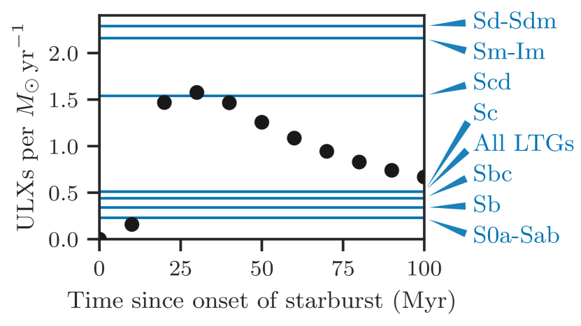
Figure 16: Formation rate of ULXs as a function of time since the onset of a star-formation episode (with constant SFR) based on the simulations of Wiktorowicz et al. (2017) for solar metallicity. The horizontal lines indicate the parameter $a$ (number of ULXs per SFR) found in different morphological types of LTGs in our sample (see Table 5). The range of $a$ in LTGs is comparable to the range of the computed formation rate of ULXs at timescales of $10-100\rm\,Myr$, except for Sd-Sdm and Sm-Im galaxies, possibly because of their sub-solar metallicity (see §§5.2, 5.3).

In the case of ETGs, most of the ULXs are expected to be long-lived systems of LMXBs with ages ${\gg}100\,\rm Myr$, but as shown in Wiktorowicz et al. (2017), the number of ULXs decreases with time since the SF episode. Therefore, the number of observed ULXs in ETGs, depends strongly on the SFH. In addition, recently, it has been shown in McDermid et al. (2015) that the age of stellar populations in ETGs can vary more than it was thought before. In order to compute a fiducial range of specific ULX frequency in ETGs, we use the average SFH of ETGs in McDermid et al. (2015) in three stellar-mass ranges: $\log{{\rm M_{\star}}}\in\left(9.5,10.0\right)$, $\left(10.0,10.5\right)$ and $\left(10.5,11.0\right)$. These ranges cover the majority of the ETGs in our sample (${\sim}90\%$).

For the three average SFHs, we compute the number of expected ULXs at the present time by convolving the SFHs (cf. Kouroumpatzakis et al. 2020) with the ULXs rates per unit stellar mass from the prediction of Wiktorowicz et al. (2017) for solar metallicity. Then, we divide by the the midpoint for each mass range in order to calculate the specific ULX frequencies in each mass range. We find 70.1, 16.7 and 5.1$\rm\,\text{ULXs per }10^{12}M_{\odot}{}$ for the low-, intermediate- and high-mass ETGs, suggesting that the ULX content of ETGs is indeed a strong function of SFH (see Figure 15). These estimates are comparable to the rates we derived from our ETGs sample, $b{=}15.1^{+3.9}_{-3.6}\rm\,\text{ULXs per }10^{12}M_{\odot}{}$ for non-AGN ETGs, and $b{=}6.3^{+1.0}_{-0.9}\rm\,\text{ULXs per }10^{12}M_{\odot}{}$ for the full ETGs sample (which is biased towards the higher mass bin; see Table 5 and Appendix B).

5.6 Limitations of this study

The parent sample of the HECATE, the HyperLEDA, includes galaxies and measurements from a multitude of surveys with different sky coverage and sensitivity. Similarly, parameters provided in HECATE (e.g., SFR, $M_{\star}$, metallicity, AGN classifications) are derived from combinations of data from all-sky surveys (e.g. IRAS, 2MASS) and the SDSS (e.g., M/L ratios, WISE forced photometry of SDSS objects). Despite the unknown selection function of the parent sample, the HECATE is the most complete sample of galaxies in the local Universe with available information on their stellar content, allowing us to draw meaningful conclusions regarding the ULX scaling relations covering a very broad stellar mass ($10^{7}.5$-$10^{11.5}\,\rm M_{\odot}$) and SFR range ($10^{-2.5}$-$10^{2}\rm\,M_{\odot}\,yr^{-1}{}$; §3.3.2).

Similarly, the serendipitous nature of the CSC 2.0 leads by definition to a non-uniform X-ray sample. In addition, to avoid contamination from X-ray emitting AGN, we exclude nuclear sources in galaxies that were either classified as AGN or we did not have information on their nuclear activity. The drawback of this approach is that we may have excluded circum-nuclear ULXs.

Finally, for the study of scaling relations, we primarily consider a secure sample of non-active galaxies to avoid the overestimation of SFR and $M_{\star}$ due to nuclear activity. This practice reduces the sample used for the ULX investigations, and may have removed known bona-fide starforming ULX hosts (e.g., Holmberg II). In addition, it leads to a bias against massive galaxies which are more likely to be targeted as AGN hosts. As discussed in §5.4, including the AGN sample, at least in the ETGs, does not bias the measured galaxy properties.

6 Summary

We construct a census of ULXs in nearby galaxies ($D{<}40\,\,\text{Mpc}{}$) by cross-matching the CSC 2.0 and the HECATE. We use this sample in order to study the ULX rates as a function of morphology, SFR, $M_{\star}$ and metallicity of their host galaxies. We deliver a sample of host galaxies and their ULX populations that serves as a benchmark for models describing the nature, formation and evolution of ULXs. We

1. constrain the number of ULXs in LTGs as a function of SFR, and both SFR and $M_{\star}$ (to account for the LMXB contribution):

   $$N_{\rm ulx} =\left(0.51\pm 0.06\right)\times\dfrac{\rm SFR}{\rm\,M_{\odot}\,yr^{-1}{}}$$ (5)

   $$N_{\rm ulx} =0.45^{+0.06}_{-0.09}\times\dfrac{\rm SFR}{\rm\,M_{\odot}\,yr^{-1}}+3.3^{+3.8}_{-3.2}\times\dfrac{M_{\star}{}}{10^{12}\,\rm M_{\odot}}.$$ (6)

2. find that the ULX-SFR scaling increases with the morphological type of LTGs.

3. verify the excess of ULXs in low-metallicity galaxies, which partially drives the above mentioned trends with the morphological type.

4. find evidence for evolution of the specific ULX frequency in ETGs with their $M_{\star}$, which we attribute to their different SFHs.

5. find that our observed scaling relations can be reproduced by published ULX formation rates from population synthesis models when accounting for the galaxies SFHs and/or metallicity.

While eROSITA (Predehl et al., 2010; Merloni et al., 2012) will provide a uniform flux-limited sample of normal galaxies and ULXs in the local Universe (e.g., Basu-Zych et al., 2020), serendipitous surveys with Chandra will continue to probe unconfused ULX populations at larger distances and their connection to the lower luminosity XRB populations.

Data availability

The data underlying this article are available in the article and in its online supplementary material.

Appendix A Galactocentric scale parameter

We define the galactocentric scale parameter, $c$, as the deprojected distance of a source from the centre of its host galaxy, normalised by the galaxy’s semi-major axis. Since the shapes of the galaxies in our study are defined through isophotal ellipses and the length of the semi-major axis is free of projection effects, we observe that $c$ can be computed as the ratio of the semi-major axes of two projected ellipses: a scaled version of the isophotal ellipse (same centre, orientation and axis ratio) passing through the source, and the isophotal ellipse itself. Consequently, for a source at $\left(\alpha_{s},\delta_{s}\right)$ and a galaxy centred at $\left(\alpha_{g},\delta_{g}\right)$ with semi-axes $R_{1},R_{2}$ and position angle $\omega$ measured from North to East, the scale $c$ is found by

1. rotating the coordinates so that the centre of the galaxy falls in $(\alpha,\delta){=}\left(0,0\right)$ and the semi-major axis is on a meridian ($a{=}0$)

2. setting the sum of the great-circle distances of the source from the focal points to be equal to two times the semi-major axis (of the scaled version of the ellipse)

Step (i) is performed by converting the spherical coordinates to Cartesian (unit radius):

$$\left(x,y,z\right)=\left(\cos\delta_{s}\cos\alpha_{s},\cos\delta_{s}\sin\alpha_{s},\sin\delta_{s}\right),$$

and rotating around the $z$-axis by $-\alpha_{g}$, the $y$-axis by $\delta_{g}$ and the $x$-axis by $-\omega$ (to align the semi-major axis with the meridian), by multiplying with the corresponding 3D-rotation matrices:

$$\begin{pmatrix}x^{\prime}\\ y^{\prime}\\ z^{\prime}\end{pmatrix}=\mathbf{R}_{x}(-\omega)\cdot\mathbf{R}_{y}(\delta_{g})\cdot\mathbf{R}_{z}(-\alpha_{g})\cdot\begin{pmatrix}x\\ y\\ z\end{pmatrix}.$$

The final coordinates are converted back to spherical coordinates:

$$\left(\alpha,\delta\right)=\left(\tan^{-1}\frac{y^{\prime}}{x^{\prime}},\frac{\pi}{2}-\cos^{-1}z^{\prime}\right).$$

Figure 17: The scaled version of the ellipse passing through the source ($P$). The separation of the source $s$ and its distance from the two focal points ($F$, $F^{\prime}$) is denoted with green dashed lines. The solid black lines denote the semi-major and semi-minor axes, while the dashed black lines indicate the distance of the co-vertex ($A$) to the focal points. The co-vertex $A$ is introduced so that the focal distance $f$ is estimated in an intermediate step.

Step (ii) consists of finding the parameters of an ellipse shown in Figure 17 for which the semi-major and semi-minor axes are scaled versions of the original ellipse $\left(r_{1},r_{2}\right){=}\left(cR_{1},cR_{2}\right)$. This is done by requiring $\left(F,P\right)+\left(F^{\prime},P\right){=}\left(F,A\right)+\left(F^{\prime},A\right)$ where $(A,B)$ denotes the great-circle distance between points $A\left(\alpha_{1},\delta_{1}\right)$ and $B\left(\alpha_{2},\delta_{2}\right)$, computed by employing a form of the Haversine formula which is more precise for nearby points:

$$s=2\sin^{-1}\sqrt{\sin^{2}\frac{\delta_{1}-\delta_{2}}{2}+\cos\delta_{1}\cos\delta_{2}\sin^{2}\frac{\alpha_{1}-\alpha_{2}}{2}}.$$

The solution in terms of $c$ (the scale of the ellipse) is found by solving for $c$ the equation:

$$\sin^{-1}\sqrt{u^{-}+w}+\sin^{-1}\sqrt{u^{+}+w}=cR_{1},$$ (7)

where

$$u^{\pm}=\sin^{2}\frac{f{\pm}\delta}{2},w=\cos f\cos\delta\sin^{2}\frac{\alpha}{2},f=\cos^{-1}\left[\frac{\cos\left(cR_{1}\right)}{\cos\left(cR_{2}\right)}\right].$$

Since the Equation 7 is not in closed form, it is solved numerically. Due to the periodicity of trigonometric functions, there are multiple solutions corresponding to ellipses engulfing the celestial sphere multiple times. To avoid this, we require that $r_{2}$ is less than $\frac{\pi}{2}$. Also, the separation of the source from the centre of the galaxy acts as a lower and upper limit for the semi-major and semi-minor axes respectively. Therefore the galactocentric distance is constrained on

$$c\in\left[\frac{s}{R_{1}},\min\left\{\frac{s}{R_{2}},\frac{\pi}{2R_{1}}\right\}\right],$$

where $s$ is now expressed in the transformed coordinates as:

$$s=2\sin^{-1}\sqrt{\sin^{2}\frac{\delta}{2}+\cos{\delta}\sin^{2}{\frac{\alpha}{2}}}.$$

Appendix B Results of fits with and without AGN hosts

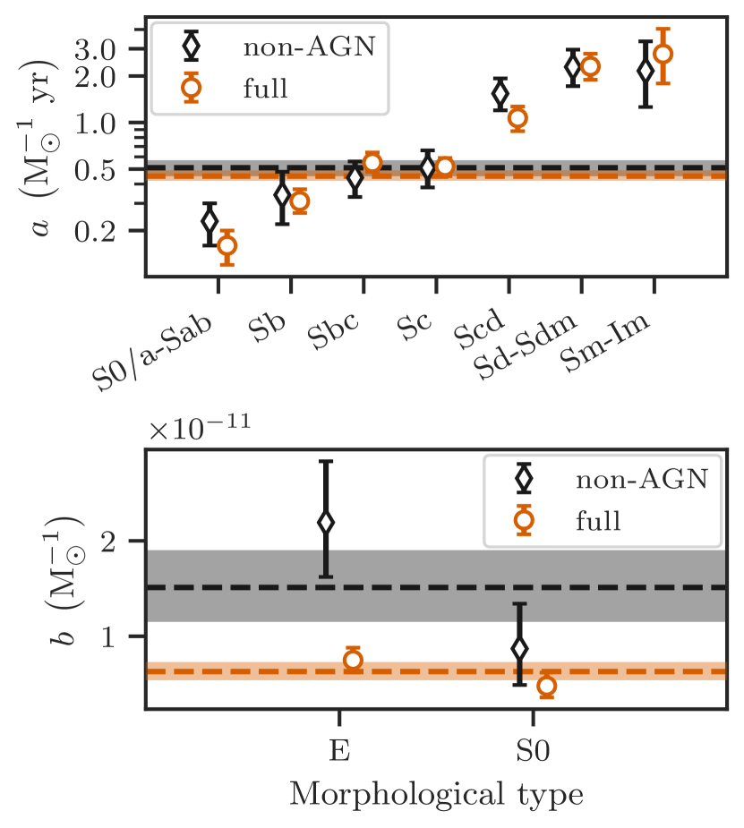
Figure 18: Comparison of fitting results between non-AGN and ‘full’ samples. Top: the scaling parameter $a$ (see Equation 2) in non-AGN LTGs (dashed black line) and its 68% CI (grey band), and in the ‘full’ sample (orange line and band). Fitting results for various morphological subclasses of LTGs are shown with errorbars. Bottom: same as top panel, but now for the scaling parameter $b$ (see Equation 1) in ETGs and separately in elliptical and lenticular galaxies.

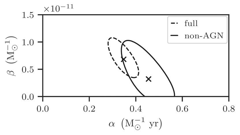
Figure 19: The best-fitting values (X symbols) and, 68% CIs (lines) of the scaling parameters $\alpha$ and $\beta$ of Equation 3, for all late-type galaxies (solid) and their non-AGN subset (dashed). The bias due to the overestimation of SFR in AGN hosts, manifests as an underestimation of the scaling parameter $\alpha$. The value of $\beta$ is highly uncertain to notice any bias due to the inclusion of AGN (lower contribution of old stellar populations in the number of ULXs in LTGs).

As described in §3.3.2, the far- and near-infrared emission from AGN may bias the estimates of SFR and $M_{\star}$ in our sample. Therefore, when fitting the models in §4.3, i.e. number of ULXs as a function of SFR and $M_{\star}$ in late- and early-type galaxies, we considered only galaxies that were classified as non-AGN in the HECATE. Here, we perform the same analysis for the complete sample (including the AGN and unclassified galaxies). The results of these fits also enable the direct comparison of this study with previous works where the AGN-hosts were not excluded from their samples.

In the following paragraphs, the complete sample without removing any AGN hosts is referred as ‘full’ sample. The sample used in §4 and §5, where galaxies with nuclear activity or lacking classification in the HECATE were excluded from the fits, is referred as ‘non-AGN’. The ‘full’ sample is larger than the ‘non-AGN’ sample by a factor of ${\sim}4$ in elliptical, ${\sim}3$ in lenticular, ${\sim}2$ in spiral and ${\sim 1.2}$ in irregular galaxies.

The top panel of Figure 18 shows the scaling of the number of ULXs with the SFR (parameter $a$ in Equation 2) in LTGs (top left) and their morphological sub-classes (top right), for the full (black) and the ‘non-AGN’ (orange) samples. We find $a=0.45^{+0.04}_{-0.03}\rm\,\text{ULXs per }M_{\odot}\,yr^{-1}{}$ in the case of the ‘full’ sample, lower than that of the ‘non-AGN’ group, $0.51{\pm}0.06\rm\,\text{ULXs per }M_{\odot}\,yr^{-1}{}$. However the difference is not significant (${\sim}1\sigma$). The comparison between the ‘non-AGN’ and ‘full’ sample for the ULX-SFR scaling in different morphological types is not conclusive because of the large uncertainties (see Figure 18).

The bottom panel of Figure 18 shows the posterior probability distribution of the scaling of the number of ULXs with $M_{\star}$ ($b$) for the ‘full’ (solid line) and ‘non-AGN’ (dashed line) ETGs. We find that the specific ULX frequency is significantly lower when ‘full’ ETGs are considered ($6.3^{+1.0}_{-0.9}\rm\,\text{ULXs per }10^{12}M_{\odot}{}$) than in the case of ‘non-AGN’ ETGs ($15^{+3.9}_{-3.6}\rm\,\text{ULXs per }10^{12}M_{\odot}$), with similar results between elliptical and lenticular galaxies.

For the scaling of the number of ULXs with SFR and $M_{\star}$ in LTGs, the posterior distribution of the two scaling factors ($\alpha$ and $\beta$) considering the ‘full’ sample is shown in Figure 19. For comparison we also show the ‘non-AGN’ case (dashed lines; presented in §4.3). We find for the 233 galaxies in the ‘full’ sample, hosting 328 ULX candidates (48.7 expected f/b sources), $\alpha=0.35^{+0.04}_{-0.05}\rm\,M_{\odot}\,yr^{-1}{}$ and $\beta=6.8^{+2.6}_{-2.2}{\times}10^{-12}\rm\,\text{ULXs per }10^{12}M_{\odot}{}$ (marginalised). The difference of the posteriors for the scaling factor $\alpha$ is consistent with the difference seen in the fits with SFR scaling only.

Given their broad-band SED, AGN may have significant contribution in the optical/UV of their host galaxies, and also in their FIR emission in the case of type-2 AGN (cf. Risaliti & Elvis 2004). However, their contribution in the near-infrared part of the spectrum is relatively small. Therefore, the difference we find in the specific ULX frequency between the ‘full’ and ‘non-AGN’ samples of ETGs is unlikely to be due to an overestimation of the $K$-band based $M_{\star}$ estimates in possible AGN in the full sample.

This is supported by the X-ray luminosities of the nuclear sources in the full ETG sample. These are very low (only one exceeds $10^{41}\,\text{erg}\,\text{s}^{-1}{}$), indicating that if there is an AGN its contribution to the $K$-band luminosity may not be significant. Additional support comes from the ratio of the nuclear and the total $K$-band luminosity in a representative sample of star-forming galaxies of Bonfini et al. (2020; submitted). This study (based on morphological decomposition of $K$-band images of the Star-Formation Reference Survey; Ashby et al. 2011) shows that the typical AGN contribution to the galactic $K$-band luminosity is ${<}10\%$. We conclude that the $M_{\star}$ estimates in AGN-hosts are not expected to be significantly biased upwards by the potential presence of an AGN.

Therefore, as discussed in §5.4, the difference in the specific ULX frequency in the non-AGN and the ‘full’ ETG samples is the result of the SFH differences in ETGs of different stellar masses.

Appendix C Detailed comparisons with previous ULX surveys

In the following subsections we compare our results with two major surveys of ULXs in the local Universe: Swartz et al. (2011) (hereafter S11) and Wang et al. (2016) (hereafter W16).

C.1 Comparison with Swartz et al. (2011)

Based on the total LTG sample in our study, we find a SFR scaling factor of ${\sim}0.51{\pm}0.06\rm\,\text{ULXs per }M_{\odot}\,yr^{-1}{}$ (see Table 5) which is ${\sim}4$ times lower than that found by S11 (${\sim}2\rm\,\text{ULXs per }M_{\odot}\,yr^{-1}{}$).

The main reason behind this discrepancy is the different samples of host galaxies in terms of morphology: S11 consider a large population of late-type and irregular galaxies, as shown in their fig. 1). Using the reported fractions of morphological types in their sample, and our fitting results for $a$ in different sub-classes of LTGs (see Table 5), we compute the expected number of ULXs in a sample with the same distribution of morphological types as in S11, based on our findings. We find $1.2\rm\,\text{ULXs per }M_{\odot}\,yr^{-1}{}$, a factor of 2.4 higher than in our sample. Another reason for this discrepancy could be differences in the X-ray photometry of the sources. Indeed, for the 99 common X-ray sources (cross-match radius of 3″), only 73 of them are characterised as ULX candidates by us, while we find that the luminosities we report are smaller by ${\sim}-0.4\rm\,dex$ (a factor of ${\sim}0.4$) compared to those computed by S11. Assuming a cumulative slope of $0.6$ (appropriate for the HMXB-LF; Grimm et al. 2003; Mineo et al. 2012), this corresponds to a lower number of ULXs by a factor of ${\sim}1.7$ compared to S11. In total, the combination of the two factors give a factor of $4.2$ lower estimate of the SFR scaling factor in our sample, explaining the difference we find.

Finally, in our sample, we find ${\sim}0.68\pm 0.10$ ULXs per elliptical galaxy (see Table 4) which is significantly higher than the rate (0.23) reported in S11. We attribute this discrepancy to the small number statistics, and the under-representation of elliptical galaxies in S11. On the other hand, the fraction of elliptical galaxies in our sample is similar to that of W16, which presents comparable number of ULXs per elliptical galaxy ($0.43{\pm}0.11$).

C.2 Comparison with Wang et al. (2016)

We cross-check the number of ULXs in our sample against the results of W16, the largest and most recent study of ULX demographics with Chandra observations. To do so, we compare the total number of ULXs in the common galaxies in our sample and in that of W16.

As a first step, we cross-match the two galaxy samples. Out of the 343 galaxies in the sample of W16, 315 are associated with our host galaxy sample. The remaining 28 galaxies are not included in our sample for various reasons. In 22 cases, the targets were observed with shallow observations (exposure times ${\lesssim{}}5\,\rm ks$) and Chandra did not detect any source. In the remaining six cases, the sources in W16 do not lie in the $D_{25}$ regions of the galaxies, our criterion for associating sources to host galaxies (NGC3066, NGC1507), or the observations were not included in the CSC 2.0 (NGC3489, NGC3489, PGC48179, PGC35286).

However, there are three additional important differences between this study and that of W16 that need to be considered in the comparison:

1. In W16, X-ray sources must exceed $2{\times}10^{39}\,\text{erg}\,\text{s}^{-1}{}$ in X-ray luminosity to be considered as ULX candidates, instead of our criterion of $L_{\rm X}{>}10^{39}\,\text{erg}\,\text{s}^{-1}{}$.

2. The X-ray source sample of W16 was taken from Liu (2011) who computed the fluxes of the sources using a count-to-flux conversion assuming a power-law spectrum with $\Gamma{=}1.7$ and Galactic line-of-sight absorption. Instead, we use the net energy of the photons as reported in the CSC 2.0 (see §3.5).

3. In this study, we associate sources to a host galaxy if they lie in its $D_{25}$ region. In W16 the $2{\times}D_{25}$ regions are used, namely the sky ellipses with twice the major and minor axes.

In order to account for the luminosity difference, we cross-match our X-ray sample with the one used by W16, and we find that our luminosities are $6\%$ smaller (median ratio; scatter of $0.5\rm\,dex$). Therefore, for this comparison only, we will consider as ULXs in our sample, the ‘reliable’ X-ray sources with $L_{\rm X}>1.89\times 10^{39}\,\text{erg}\,\text{s}^{-1}{}$ to account for the above mentioned luminosity offset. We find a total of 186 ULX candidates in our sample. The same luminosity limit is used to calculate the expected foreground/background contamination (see §3.6), for which we find 37.9 sources, leading to a final estimate of 148.1 ULXs in the 315 galaxies, based on our emulation of the W16 sample.

To correct for the difference between the number of sources in the $D_{25}$ and $2{\times}D_{25}$ regions, we cross-match the X-ray sample with the HECATE and find that the number of X-ray sources that lie in the $2{\times}D_{25}$ regions is $35\%$ larger than the number of sources in the $D_{25}$ regions. Therefore, the number of ULX candidates in the $2{\times}D_{25}$ regions, 215, as reported in W16, corresponds to about 159.3 candidates in the $D_{25}$ regions. By subtracting one forth of the, reported by W16, number of interlopers (since the area of the $D_{25}$ regions is four times than the area of the $2{\times}D_{25}$ regions), we find that the number of ULXs in the $D_{25}$ regions is 151.1, close to the value we find in our sample (148.1).

Lastly, the ULX rates above 2, 3, 5 and 10$\times 10^{39}\,\text{erg}\,\text{s}^{-1}{}$ in the different morphological types in our sample (see Table 4) are consistent at the $2\sigma$-level with the rates found in the table 2 in W16.

References

- Abramowicz et al. (1988) Abramowicz M. A., Czerny B., Lasota J. P., Szuszkiewicz E., 1988, ApJ, 332, 646
- Anastasopoulou et al. (2016) Anastasopoulou K., Zezas A., Ballo L., Della Ceca R., 2016, MNRAS, 460, 3570
- Anastasopoulou et al. (2019) Anastasopoulou K., Zezas A., Gkiokas V., Kovlakas K., 2019, MNRAS, 483, 711
- Angelini et al. (2001) Angelini L., Loewenstein M., Mushotzky R. F., 2001, ApJ, 557, L35
- Antoniou & Zezas (2016) Antoniou V., Zezas A., 2016, MNRAS, 459, 528
- Antoniou et al. (2019) Antoniou V., et al., 2019, ApJ, 887, 20
- Ashby et al. (2011) Ashby M. L. N., et al., 2011, PASP, 123, 1011
- Bachetti et al. (2014) Bachetti M., et al., 2014, Nature, 514, 202
- Basu-Zych et al. (2013a) Basu-Zych A. R., et al., 2013a, ApJ, 762, 45
- Basu-Zych et al. (2013b) Basu-Zych A. R., et al., 2013b, ApJ, 774, 152
- Basu-Zych et al. (2016) Basu-Zych A. R., Lehmer B., Fragos T., Hornschemeier A., Yukita M., Zezas A., Ptak A., 2016, ApJ, 818, 140
- Basu-Zych et al. (2020) Basu-Zych A. R., et al., 2020, arXiv e-prints, p. arXiv:2008.01870
- Begelman (2002) Begelman M. C., 2002, ApJ, 568, L97
- Belczynski et al. (2010) Belczynski K., Bulik T., Fryer C. L., Ruiter A., Valsecchi F., Vink J. S., Hurley J. R., 2010, ApJ, 714, 1217
- Bell et al. (2003) Bell E. F., McIntosh D. H., Katz N., Weinberg M. D., 2003, ApJS, 149, 289
- Berger (2014) Berger E., 2014, ARA&A, 52, 43
- Brandt & Alexander (2015) Brandt W. N., Alexander D. M., 2015, A&ARv, 23, 1
- Brinchmann et al. (2004) Brinchmann J., Charlot S., White S. D. M., Tremonti C., Kauffmann G., Heckman T., Brinkmann J., 2004, MNRAS, 351, 1151
- Brorby et al. (2014) Brorby M., Kaaret P., Prestwich A., 2014, MNRAS, 441, 2346
- Brorby et al. (2016) Brorby M., Kaaret P., Prestwich A., Mirabel I. F., 2016, MNRAS, 457, 4081
- Carpano et al. (2018) Carpano S., Haberl F., Maitra C., Vasilopoulos G., 2018, MNRAS, 476, L45
- Cluver et al. (2017) Cluver M. E., Jarrett T. H., Dale D. A., Smith J.-D. T., August T., Brown M. J. I., 2017, ApJ, 850, 68
- Colbert & Mushotzky (1999) Colbert E. J. M., Mushotzky R. F., 1999, ApJ, 519, 89
- Colbert & Ptak (2002) Colbert E. J. M., Ptak A. F., 2002, ApJS, 143, 25
- Dage et al. (2020) Dage K. C., Zepf S. E., Thygesen E., Bahramian A., Kundu A., Maccarone T. J., Peacock M. B., Strader J., 2020, MNRAS, 497, 596
- Dale & Helou (2002) Dale D. A., Helou G., 2002, ApJ, 576, 159
- Das et al. (2017) Das A., Mesinger A., Pallottini A., Ferrara A., Wise J. H., 2017, MNRAS, 469, 1166
- David et al. (2005) David L. P., Jones C., Forman W., Murray S. S., 2005, ApJ, 635, 1053
- Delvecchio et al. (2020) Delvecchio I., et al., 2020, ApJ, 892, 17
- Douna et al. (2015) Douna V. M., Pellizza L. J., Mirabel I. F., Pedrosa S. E., 2015, A&A, 579, A44
- Earnshaw et al. (2019) Earnshaw H. P., Roberts T. P., Middleton M. J., Walton D. J., Mateos S., 2019, MNRAS, 483, 5554
- Elmegreen & Falgarone (1996) Elmegreen B. G., Falgarone E., 1996, ApJ, 471, 816
- Eracleous et al. (2002) Eracleous M., Shields J. C., Chartas G., Moran E. C., 2002, ApJ, 565, 108
- Evans et al. (2010) Evans I. N., et al., 2010, ApJS, 189, 37
- Fabbiano (1989) Fabbiano G., 1989, ARA&A, 27, 87
- Fabbiano et al. (2001) Fabbiano G., Zezas A., Murray S. S., 2001, ApJ, 554, 1035
- Fabbiano et al. (2006) Fabbiano G., et al., 2006, ApJ, 650, 879
- Farrell et al. (2009) Farrell S. A., Webb N. A., Barret D., Godet O., Rodrigues J. M., 2009, Nature, 460, 73
- Feng & Kaaret (2008) Feng H., Kaaret P., 2008, ApJ, 675, 1067
- Finke & Razzaque (2017) Finke J. D., Razzaque S., 2017, MNRAS, 472, 3683
- Fornasini et al. (2019) Fornasini F. M., et al., 2019, ApJ, 885, 65
- Fornasini et al. (2020) Fornasini F. M., Civano F., Suh H., 2020, MNRAS,
- Fragos et al. (2013a) Fragos T., et al., 2013a, ApJ, 764, 41
- Fragos et al. (2013b) Fragos T., Lehmer B. D., Naoz S., Zezas A., Basu-Zych A., 2013b, ApJ, 776, L31
- Fragos et al. (2015) Fragos T., Linden T., Kalogera V., Sklias P., 2015, ApJ, 802, L5
- Fürst et al. (2016) Fürst F., et al., 2016, ApJ, 831, L14
- Gao et al. (2003) Gao Y., Wang Q. D., Appleton P. N., Lucas R. A., 2003, ApJ, 596, L171
- Ghosh et al. (2008) Ghosh H., Mathur S., Fiore F., Ferrarese L., 2008, ApJ, 687, 216
- Gladstone et al. (2009) Gladstone J. C., Roberts T. P., Done C., 2009, MNRAS, 397, 1836
- Gong et al. (2016) Gong H., Liu J., Maccarone T., 2016, ApJS, 222, 12
- González Delgado et al. (2015) González Delgado R. M., et al., 2015, A&A, 581, A103
- Greiner et al. (2001) Greiner J., Cuby J. G., McCaughrean M. J., Castro-Tirado A. J., Mennickent R. E., 2001, A&A, 373, L37
- Grimm et al. (2003) Grimm H.-J., Gilfanov M., Sunyaev R., 2003, MNRAS, 339, 793
- Heger et al. (2003) Heger A., Fryer C. L., Woosley S. E., Langer N., Hartmann D. H., 2003, ApJ, 591, 288
- Helou & Walker (1988) Helou G., Walker D. W., 1988, in NASA RP-1190, Vol. 7 (1988).
- Ho et al. (2001) Ho L. C., et al., 2001, ApJ, 549, L51
- Israel et al. (2017a) Israel G. L., et al., 2017a, Science, 355, 817
- Israel et al. (2017b) Israel G. L., et al., 2017b, MNRAS, 466, L48
- Kaaret et al. (2004) Kaaret P., Alonso-Herrero A., Gallagher J. S., Fabbiano G., Zezas A., Rieke M. J., 2004, MNRAS, 348, L28
- Kaaret et al. (2017) Kaaret P., Feng H., Roberts T. P., 2017, ARA&A, 55, 303
- Kauffmann et al. (2003) Kauffmann G., et al., 2003, MNRAS, 346, 1055
- Kennicutt (1998) Kennicutt Jr. R. C., 1998, ARA&A, 36, 189
- Kennicutt & Evans (2012) Kennicutt R. C., Evans N. J., 2012, ARA&A, 50, 531
- Kewley & Ellison (2008) Kewley L. J., Ellison S. L., 2008, ApJ, 681, 1183
- Kim & Fabbiano (2004) Kim D.-W., Fabbiano G., 2004, ApJ, 611, 846
- Kim & Fabbiano (2010) Kim D.-W., Fabbiano G., 2010, ApJ, 721, 1523
- Kim et al. (2006) Kim E., Kim D.-W., Fabbiano G., Lee M. G., Park H. S., Geisler D., Dirsch B., 2006, ApJ, 647, 276
- Kim et al. (2007) Kim M., Wilkes B. J., Kim D.-W., Green P. J., Barkhouse W. A., Lee M. G., Silverman J. D., Tananbaum H. D., 2007, ApJ, 659, 29
- King & Lasota (2016) King A., Lasota J.-P., 2016, MNRAS, 458, L10
- King et al. (2001) King A. R., Davies M. B., Ward M. J., Fabbiano G., Elvis M., 2001, ApJ, 552, L109
- King et al. (2017) King A., Lasota J.-P., Kluźniak W., 2017, MNRAS, 468, L59
- Koliopanos et al. (2019) Koliopanos F., Vasilopoulos G., Buchner J., Maitra C., Haberl F., 2019, A&A, 621, A118
- Kouroumpatzakis et al. (2020) Kouroumpatzakis K., et al., 2020, MNRAS, 494, 5967
- Kuranov et al. (2007) Kuranov A. G., Popov S. B., Postnov K. A., Volonteri M., Perna R., 2007, MNRAS, 377, 835
- Lang et al. (2016) Lang D., Hogg D. W., Schlegel D. J., 2016, AJ, 151, 36
- Lehmer et al. (2005) Lehmer B. D., et al., 2005, AJ, 129, 1
- Lehmer et al. (2016) Lehmer B. D., et al., 2016, ApJ, 825, 7
- Lehmer et al. (2019) Lehmer B. D., et al., 2019, ApJS, 243, 3
- Linden et al. (2010) Linden T., Kalogera V., Sepinsky J. F., Prestwich A., Zezas A., Gallagher J. S., 2010, ApJ, 725, 1984
- Liu (2011) Liu J., 2011, ApJS, 192, 10
- Liu et al. (2006) Liu J.-F., Bregman J. N., Irwin J., 2006, ApJ, 642, 171
- Long & van Speybroeck (1983) Long K. S., van Speybroeck L. P., 1983, in Lewin W. H. G., van den Heuvel E. P. J., eds, Accretion-Driven Stellar X-ray Sources. pp 117–146
- Maccarone et al. (2007) Maccarone T. J., Kundu A., Zepf S. E., Rhode K. L., 2007, Nature, 445, 183
- Madau & Dickinson (2014) Madau P., Dickinson M., 2014, ARA&A, 52, 415
- Madau & Fragos (2017) Madau P., Fragos T., 2017, ApJ, 840, 39
- Madau et al. (2004) Madau P., Rees M. J., Volonteri M., Haardt F., Oh S. P., 2004, ApJ, 604, 484
- Makarov et al. (2014) Makarov D., Prugniel P., Terekhova N., Courtois H., Vauglin I., 2014, A&A, 570, A13
- Makishima et al. (2000) Makishima K., et al., 2000, ApJ, 535, 632
- Mapelli et al. (2010) Mapelli M., Ripamonti E., Zampieri L., Colpi M., Bressan A., 2010, MNRAS, 408, 234
- Mapelli et al. (2011) Mapelli M., Ripamonti E., Zampieri L., Colpi M., 2011, Astronomische Nachrichten, 332, 414
- Maragkoudakis et al. (2017) Maragkoudakis A., Zezas A., Ashby M. L. N., Willner S. P., 2017, MNRAS, 466, 1192
- Marchant et al. (2017) Marchant P., Langer N., Podsiadlowski P., Tauris T. M., de Mink S., Mandel I., Moriya T. J., 2017, A&A, 604, A55
- McDermid et al. (2015) McDermid R. M., et al., 2015, MNRAS, 448, 3484
- Merloni et al. (2012) Merloni A., et al., 2012, arXiv e-prints, p. arXiv:1209.3114
- Middleton & King (2017) Middleton M. J., King A., 2017, MNRAS, 470, L69
- Middleton et al. (2015) Middleton M. J., Heil L., Pintore F., Walton D. J., Roberts T. P., 2015, MNRAS, 447, 3243
- Mineo et al. (2012) Mineo S., Gilfanov M., Sunyaev R., 2012, MNRAS, 419, 2095
- Misra et al. (2020) Misra D., Fragos T., Tauris T., Zapartas E., Aguilera-Dena D. R., 2020, arXiv e-prints, p. arXiv:2004.01205
- Mondal et al. (2020) Mondal S., Belczyński K., Wiktorowicz G., Lasota J.-P., King A. R., 2020, MNRAS, 491, 2747
- Mullaney et al. (2011) Mullaney J. R., Alexander D. M., Goulding A. D., Hickox R. C., 2011, MNRAS, 414, 1082
- Park et al. (2006) Park T., Kashyap V. L., Siemiginowska A., van Dyk D. A., Zezas A., Heinke C., Wargelin B. J., 2006, ApJ, 652, 610
- Pettini & Pagel (2004) Pettini M., Pagel B. E. J., 2004, MNRAS, 348, L59
- Pilyugin (2001) Pilyugin L. S., 2001, A&A, 369, 594
- Pilyugin & Thuan (2005) Pilyugin L. S., Thuan T. X., 2005, ApJ, 631, 231
- Plotkin et al. (2014) Plotkin R. M., Gallo E., Miller B. P., Baldassare V. F., Treu T., Woo J.-H., 2014, ApJ, 780, 6
- Predehl et al. (2010) Predehl P., et al., 2010, in Space Telescopes and Instrumentation 2010: Ultraviolet to Gamma Ray. p. 77320U (arXiv:1001.2502), doi:10.1117/12.856577
- Prestwich et al. (2013) Prestwich A. H., Tsantaki M., Zezas A., Jackson F., Roberts T. P., Foltz R., Linden T., Kalogera V., 2013, ApJ, 769, 92
- Ptak & Griffiths (1999) Ptak A., Griffiths R., 1999, ApJ, 517, L85
- Rappaport et al. (2005) Rappaport S. A., Podsiadlowski P., Pfahl E., 2005, MNRAS, 356, 401
- Raychaudhury et al. (2008) Raychaudhury S., Vargas I. M., Jones C., Forman W. R., Vikhlinin A., Murray S. S., 2008, in Chakrabarti S. K., Majumdar A. S., eds, American Institute of Physics Conference Series Vol. 1053, American Institute of Physics Conference Series. pp 111–115, doi:10.1063/1.3009468
- Remillard & McClintock (2006) Remillard R. A., McClintock J. E., 2006, ARA&A, 44, 49
- Risaliti & Elvis (2004) Risaliti G., Elvis M., 2004, A Panchromatic View of AGN. Barger, A. J., p. 187, doi:10.1007/978-1-4020-2471-9_6
- Roberts & Warwick (2000) Roberts T. P., Warwick R. S., 2000, MNRAS, 315, 98
- Roberts et al. (2002) Roberts T. P., Warwick R. S., Ward M. J., Murray S. S., 2002, MNRAS, 337, 677
- Rodighiero et al. (2011) Rodighiero G., et al., 2011, ApJ, 739, L40
- Rowan-Robinson (1999) Rowan-Robinson M., 1999, Ap&SS, 266, 291
- She et al. (2017) She R., Ho L. C., Feng H., 2017, ApJ, 835, 223
- Sądowski et al. (2014) Sądowski A., Narayan R., McKinney J. C., Tchekhovskoy A., 2014, MNRAS, 439, 503
- Soria et al. (2005) Soria R., Cropper M., Pakull M., Mushotzky R., Wu K., 2005, MNRAS, 356, 12
- Speagle et al. (2014) Speagle J. S., Steinhardt C. L., Capak P. L., Silverman J. D., 2014, ApJS, 214, 15
- Stampoulis et al. (2019) Stampoulis V., van Dyk D. A., Kashyap V. L., Zezas A., 2019, MNRAS, 485, 1085
- Steer et al. (2017) Steer I., et al., 2017, AJ, 153, 37
- Sun et al. (2018) Sun N.-C., et al., 2018, ApJ, 858, 31
- Svoboda et al. (2019) Svoboda J., Douna V., Orlitová I., Ehle M., 2019, ApJ, 880, 144
- Swartz et al. (2004) Swartz D. A., Ghosh K. K., Tennant A. F., Wu K., 2004, ApJS, 154, 519
- Swartz et al. (2008) Swartz D. A., Soria R., Tennant A. F., 2008, ApJ, 684, 282
- Swartz et al. (2011) Swartz D. A., Soria R., Tennant A. F., Yukita M., 2011, ApJ, 741, 49
- Tremonti et al. (2004) Tremonti C. A., et al., 2004, ApJ, 613, 898
- Tzanavaris et al. (2016) Tzanavaris P., Hornschemeier A. E., Gallagher S. C., Lenkić L., Desjardins T. D., Walker L. M., Johnson K. E., Mulchaey J. S., 2016, ApJ, 817, 95
- Venkatesan et al. (2001) Venkatesan A., Giroux M. L., Shull J. M., 2001, ApJ, 563, 1
- Walton et al. (2011) Walton D. J., Roberts T. P., Mateos S., Heard V., 2011, MNRAS, 416, 1844
- Walton et al. (2019) Walton D. J., et al., 2019, MNRAS, 484, 2544
- Wang et al. (2016) Wang S., Qiu Y., Liu J., Bregman J. N., 2016, ApJ, 829, 20
- Wiktorowicz et al. (2017) Wiktorowicz G., Sobolewska M., Lasota J.-P., Belczynski K., 2017, ApJ, 846, 17
- Wolter & Trinchieri (2004) Wolter A., Trinchieri G., 2004, A&A, 426, 787
- Wolter et al. (2018) Wolter A., Fruscione A., Mapelli M., 2018, ApJ, 863, 43
- Zezas et al. (2003) Zezas A., Ward M. J., Murray S. S., 2003, ApJ, 594, L31
- Zezas et al. (2007) Zezas A., Fabbiano G., Baldi A., Schweizer F., King A. R., Rots A. H., Ponman T. J., 2007, ApJ, 661, 135
- Zhang et al. (2012) Zhang Z., Gilfanov M., Bogdán Á., 2012, A&A, 546, A36
- de Vaucouleurs (1991) de Vaucouleurs G., 1991, Science, 254, 592
- de Vaucouleurs et al. (1976) de Vaucouleurs G., de Vaucouleurs A., Corwin J. R., 1976, in Second reference catalogue of bright galaxies, Vol. 1976, p. Austin: University of Texas Press..
- van der Marel (2004) van der Marel R. P., 2004, Coevolution of Black Holes and Galaxies, p. 37