Mathematical and Computer Modeling of COVID-19 Transmission Dynamics in Bulgaria by Time-depended Inverse SEIR Model

Abstract.

Since the end of 2019, with the outbreak of the new virus COVID-19, the world changed entirely in many aspects, with the pandemia affecting the economies, healthcare systems and the global socium. As a result from this pandemic, scientists from many countries across the globe united in their efforts to study the virsus’s behavior and are attempting to predict mathematically its infection model in order to limit its impact and developing new methods and models to achieve this goal. In this paper we explore a time-depended SEIR model, in which the dynamics of the infection in four groups from a selected target group (population), divided according to the infection, are modeled by a system of nonlinear ordinary differential equations. Several basic parameters are involved in the model: coefficients of infection rate, incubation rate, recovery rate. The coefficients are adaptable to each specific infection, for each individual country, and depend on the measures to limit the spread of the infection and the effectiveness of the methods of treatment of the infected people in the respective country. If such coefficients are known, solving the nonlinear system is possible to be able to make some hypotheses for the development of the epidemic. This is the reason for using Bulgarian COVID-19 data to first of all, solve the so-called ”inverse problem” and to find the parameters of the current situation. Reverse logic is initially used to determine the parameters of the model as a function of time, followed by computer solution of the problem. Namely, this means predicting the future behavior of these parameters, and finding (and as a consequence applying mass-scale measures, e.g., distancing, disinfection, limitation of public events), a suitable scenario for the change in the proportion of the numbers of the four studied groups in the future. In fact, based on these results we model the COVID-19 transmission dynamics in Bulgaria and make a two-week forecast for the numbers of new cases per day, active cases and recovered individuals. Such model, as we show, has been successful for prediction analysis in the Bulgarian situation. We also provide multiple examples of numerical experiments with visualization of the results.

1. Introduction

1.1. The Pandemic of SARS-CoV-2 - worldwide and in Bulgaria

On 31st of December 2019, the Chinese Centre for Disease Control and Prevention (China CDC) informed the World Health Organization (WHO) about a cluster of 41 severe pneumonia cases of unknown aetiology in Wuhan, Hubei province. A newly identified $\beta$-coronavirus (whole genome sequenced on 5th of January and isolated on 7th of January) was initially named 2019-nCoV (2019-novel CoronaVirus/12 January 2020) and later renamed to SARS-CoV-2 (Severe Acute Respiratory Syndrome CoronaVirus -2/12 February 2020) by the Coronavirus Study Group of the International Committee on Taxonomy of Viruses [1]. The extensive global transmission led to the declaring coronavirus disease of 2019 (COVID-19) as a pandemic with significant mortality and morbidity [2]. By 27 February 2020, the outbreak of coronavirus disease 2019 (COVID-19) caused 13 285 640 confirmed cases and 578 110 deaths globally, more than severe acute respiratory syndrome (SARS) (8273 cases, 775 deaths) and Middle East respiratory syndrome (MERS) (1139 cases, 431 deaths) caused in 2003 and 2013, respectively. COVID-19 has spread to 216 countries internationally. Total fatality rate of COVID-19 is estimated at 3.46% by far based on published data from China CDC. Average incubation period of COVID-19 is around 6.4 days, ranges from 0 to 14 days. The basic reproductive number ($\Re_{0}$) of COVID-19 ranges from 2 to 3.5 at the early phase regardless of different prediction models, which is higher than SARS and MERS [3]. The epidemiological and clinical data collected so far suggest that the disease spectrum of COVID-19 may differ from SARS or MERS. Person-to-person transmission of COVID-19 infection led to the isolation of patients that were subsequently administered a variety of treatments. Extensive measures to reduce person-to-person transmission of COVID-19 have been implemented to control the current outbreak and this has led to a significant reduction in the viral spread and a reduction in new cases. In Bulgaria, the disease began with a limited number of cases. The government took instant, timely and decisive measures, which led to a reduction in the spread of the infection. There was a weak first wave with a peak around April 20, when the new cases reached 91 per a day. There was a clear decrease in morbidity over the next month and a half, of which, due to the implemented measures. After restrictions were lifted and borders were opened, cases began to rise rapidly and right now Bulgaria is in ”second” wave, with the intensity of morbidity of around of 250 new cases per a day. A very similar picture could be seen in the rest of Europe, where the mitigation of measures and lifting of the travel restrictions had also led to a rapid increase in the number of positive cases and morbidity rates. A major part of the special efforts to predict, prevent and reduce the transmission of the disease, is to develop a mathematic-computation model for forecasting the COVID - 19 spread in Bulgaria in Europe and in the world wide.

1.2. Epidemic Dynamics Modeling and Analysis

The modern approach for studying and forecasting the dynamics of pandemic processes is connected to the use of deterministic mathematical models described by differential equations. They track the quantitative changes over time of main population groups representing different stages of the course of the disease or pandemic (virus carriers, hospitalized, recovered, etc.). The equations in the mathematical models describe the consecution and velocity of transitions from one group to another. The exact dependencies in the equations are controlled by coefficients that take into account the real (measurable) characteristics of the infectious disease and the human population in the respective region and are determined by the empirical data. The most commonly used models, including for predicting the current COVID-19 pandemic, are based on the so-called SIR and SEIR models, which are essentially systems of nonlinear ordinary differential equations. Specifically for COVID-19, see, for example, the Chris Murray Model [4], the Epidemic Calculator [5], and the works [6, 7] of Neil Ferguson, Imperial College, London. The same model has been used also to analyze the situation in China [8]. For more detailed and complied analysis see a newly published monograph [9].

The mathematical and computer modeling of the COVID-19 pandemic is a really interesting and important topic in which mathematical modeling and high - performance computational calculations clearly cooperate. This is a modern tool not only for forecasting, but also for studying the mechanisms of disease spread, for assessing the effect of various interventions or strategies for controlling the pandemic.

In SEIR model the host population is represented by the following compartments:

• Susceptible individuals $S(t)$. These are the people who may be infected and can become virus carriers. Usually at the beginning of the pandemic, as in the case on COVID-19, the whole population of the country is susceptible.

• Exposed individuals $E(t)$. These are virus carriers individuals in the latent stage, during which they are not virus spreaders. They usually have no symptoms.

• Infectious individuals $I(t)$. These are the individuals who are with strong infectivity virus carriers and virus spreaders. These are the people who may be passing the virus on to others in case of contact. It is supposed that at the start there is at least one infectious individual.

• Recovered individuals $R(t)$. These are the recovered from the disease individuals (in the same group we calculate also the deceased individuals).

The total population size is supposed to be a constant $N=S(t)+E(t)+I(t)+R(t)$ during the considered pandemic period.

In SEIR model the quantitative changes over time are described by the following Cauchy problem for system of nonlinear ordinary differential equations (under assumptions that $S(t),\,E(t),\,I(t)$ and $R(t)$ are differentiable functions):

(1) $$\text{SEIR model:}\left|\begin{array}[]{l}\displaystyle{\frac{dS}{dt}}=-\frac{\beta}{N}S(t)I(t),\\ \\ \displaystyle{\frac{dE}{dt}}=\frac{\beta}{N}S(t)I(t)-\omega E(t),\\ \\ \displaystyle{\frac{dI}{dt}}=\omega E(t)-\gamma I(t),\\ \\ \displaystyle{\frac{dR}{dt}}=\gamma I(t),\\ \\ S(0)=S_{0},\,E(0)=E_{0},\,I(0)=I_{0},\,R(0)=R_{0},\end{array}\right.$$

Here $S_{0}>0,\,E_{0}\geq 0,\,I_{0}>0,\,R_{0}\geq 0$ are the initial numbers of individuals in the fourth compartments. The model involves three parameters:

• Infection (transmission) rate $\beta$ of the biological epidemic, which is a product of the of contact rate $r$ between people in the population and the probability of transmission $\beta_{0}$ upon contact between an Infectious individual and a Susceptible individual;

• Latent (incubation) rate $\omega=\frac{1}{T_{e}},$ where $T_{e}$ denoted average latency time (incubation period).

• Rate of the Infectious people transform to the Recovered people, i.e. recovery rate $\gamma=\frac{1}{T_{i}},$ where $T_{i}$ denoted the average recovery time.

A fundamental concept in epidemiology is the basic reproduction number $\Re_{0}$, which measures the speed of spread of an infectious disease. In SEIR model (1) (see [10, 11]) it is

(2) $$\Re_{0}=\frac{\beta}{\gamma}.$$

When $\Re_{0}>1$ the speed of spread is positive and SEIR model gives exponential growth of infectious individuals. If $\Re_{0}=1$, then the speed of spread is zero (disease threshold). If $\Re_{0}<1$ the spread speed is negative and the infection subsides.

SEIR model (1) can be considered as generalization of the SIR model, suggested by Kermack and McKendrick [12]. SIR model has been widely applied in dynamic transmission modeling of a directly transmitted pathogen such as influenza. The latent period is ignored and the compartment of Exposed individuals absents in it:

(3) $$\text{SIR model:}\left|\begin{array}[]{l}\displaystyle{\frac{dS}{dt}}=-\frac{\beta_{1}}{N}S(t)I(t),\\ \\ \displaystyle{\frac{dI}{dt}}=\frac{\beta_{1}}{N}S(t)I(t)-\gamma_{1}I(t),\\ \\ \displaystyle{\frac{dR}{dt}}=\gamma_{1}I(t),\\ \\ S(0)=S_{0},\,I(0)=I_{0},\,R(0)=R_{0}.\end{array}\right.$$

Here the parameters are the infection rate $\beta_{1}$ and the recovery rate $\gamma_{1}$. The basic reproduction number $\Re_{0}$ in SIR model (3) is defined as the ratio of the infection rate $\beta_{1}$ to recovery rate $\gamma_{1}.$

Remark 1.

Let us mention here the difference between both Models: In SEIR model there are four different groups of people, instead of three in SIR. This difference is very important because to solve the inverse problem of finding the coefficients $\beta,\,\omega$ and $\gamma$ in SEIR model we need more information, than in SIR, which unfortunately is not public. With this reason to solve this problem we are going in a different way (see Section 2). Let us also mention some other models, which are more advanced. For example see SEIQRS Epidemic Diffusion Model (see Liu, Cao, Liang, Chen monograph [9], 2020). What is the difference with SEIR model for example there? In SEIQRS model there is one more compartment of Quarantined individuals and it is supposed that recovered people have not immunity. If we look to the first equation in SIR or in SEIR model, there is a product $S(t)I(t)$ which actually means that the number of susceptible people depends on the number of meetings between the all people $S(t)$ and all infectious cases $I(t)$. Instead of this, in SEIQRS model [9] this product has been changed with the product $S(t)I_{1}(t)$, where $I_{1}(t)$ is the number of another group of people, infective with strong infectivity, which have not yet been quarantined. This model is obviously more accurate; however, due to lack of publicly accessible data, this is not applicable in Bulgaria for research purposes. If the researchers had more accurate data on the number of quarantined individuals, it would have been possible to make more accurate forecasts.

The SIR and SEIR models with constant coefficients are useful for modeling of rapid spread of disease to a large number of people in a given population within a short period of time (see [13]). Seasonal epidemics or controlled pandemic by a switching prevention strategy, which may include vaccination and outbreak control measures are described by models with time-depended transmission parameters (see [14, 15, 16] ). In these cases the number of infectious individuals $I(t)$ can have many local maxima (see Figure 1 (b)), instead of one pick (in the cases of constant coefficients, Figure 1 (a)), and they can be controlled by good prevention strategy.

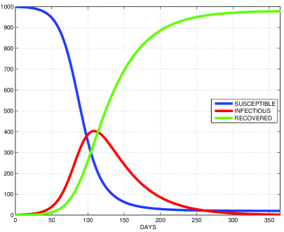
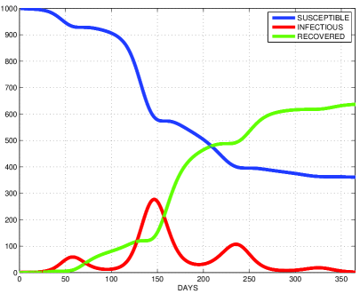
(a) constant coefficients		(b) time-depended coefficients

Figure 1. SIR model infectious curve (in red) with one (a) or several (b) maxima.

As is mentioned in [8] the value of the infection rate $\beta$ can be changed by various government control measures. For example, educational facilities closing, gathering restrictions, travel restrictions, cancelation of mass gatherings, and similar control measures impact on the values of of the rate $r$ of contact between people in the population. On the other hand, the recovery rate $\gamma$ can be changed, for example, by methodological improvement on the diagnosis and treatment strategy. Therefore it is reasonable to use time-depended models to describe the COVID-19 pandemic dynamics.

1.3. Spatial Dynamics

The spatial disease dynamics is among the challenging topics to better understanding of future development of COVID-19 and other related pandemics, due to the ever stronger impact of human mobility to infectious disease dynamics on larger geographical scales. For SEIR model, this means generalization of the basic system of ordinary differential equations to systems of either integral equations, partial differential equations or coupled ordinary differential equations on a weighted graph, thus including the spatial diffusion (see, e.g., [17, 18, 19, 20]). At a certain level of epidemic development, the long range human mobility is responsible for the rapid geographical spread of emergent infectious diseases, thus violating the Brownian motion hypotheses. Although significantly more complex, the emerging fractional diffusion models provide new opportunities for better analysis of such non-local phenomena. The successful development of spatial time-depended inverse SEIR models will require substantially bigger amount and more reliable data to determine the related coefficients, which are by default strongly heterogeneous in space. The data for time-dependent density of individuals is just one of the challenges. For example, in the numerical tests presented in [17], data for the flux of dollar bills in US is used to parametrize the model of spatial dynamics. The analysis of spatial dynamics of epidemic diseases is a topic with great social and economic impact. The common understanding of this is rapidly increasing during the ongoing COVID-19 pandemic. This is convincingly supported by the following example. The Institute for Health Metrics and Evaluation (IHME) is an independent research center at the University of Washington, financially supported by the Bill & Melinda Gates Foundation [21]. For the next decade, IHME has formulated the following ambitious target: ”Scale up our geospatial analyses toward our aspiration of mapping all diseases, risks, and covariates at 5 km by 5 km resolution or better.” In the spirit spatial SEIR models, such (or even coarser) resolution can be achieved only via deep synergy of resources in High Performance Computing (HPC) and Artificial Intelligence (AI) in Big Data environment.

The paper is organized as follows. In Section 2 we introduce a time-depended inverse SEIR model for daily adjustment of the infection, latent, and the recovery rates. Additionally, we propose difference schemes for numerically solving the corresponding direct and inverse problems. In Section 3 this theoretical machinery is used for experimental analysis of the pandemic situation in Bulgaria and for a development of a strategy for mid-time-frame forecasting. Numerical results for three different 14-days-periods are documented and analyzed. Conclusions are outlined in Section 4.

2. COVID-19 spread modeling by time-depended inverse SEIR model

In this section we consider SEIR model with time depended parameters:

(4) $$\text{TD-SEIR model:}\left|\begin{array}[]{l}\displaystyle{\frac{dS}{dt}}=-\frac{\beta(t)}{N}S(t)I(t),\\ \\ \displaystyle{\frac{dE}{dt}}=\frac{\beta(t)}{N}S(t)I(t)-\omega(t)E(t),\\ \\ \displaystyle{\frac{dI}{dt}}=\omega(t)E(t)-\gamma(t)I(t),\\ \\ \displaystyle{\frac{dR}{dt}}=\gamma(t)I(t),\\ \\ S(0)=S_{0},\,E(0)=E_{0},\,I(0)=I_{0},\,R(0)=R_{0}.\end{array}\right.$$

The parameters in TD-SEIR model (4) are different in different stages of pandemic and they are specifically for each country. We assume that $\omega(t)=1/T_{e}(t)\leq 1$ and $\gamma(t)=1/T_{i}(t)\leq 1,$ where $T_{e}(t)$ and $T_{i}(t)$ are average latency time and average recovery time to the moment $t$.

One can solve the Cauchy problem in TD-SEIR model (4) knowing the initial data and the value of the parameters. In such way functions describing the quantitative changes in considered compartment of population can be found. But this is not the case. Official data sources relating to the COVID-19 pandemic contains information only for number of active cases and number of Recovered individuals $R(t)$. Since many people who have the disease show no symptoms it is reasonable to assume that active cases are infectious and exposed individuals and will denote them by $A(t)=E(t)+I(t).$ The parameters in the TD-SEIR model (4) are unknown and therefore in order to study the COVID-19 pandemic dynamics the first step is to solve

The inverse problem: To find the parameters $\beta(t),\,\omega(t)$ and $\gamma(t)$ in the TD-SEIR model (4) using the knowing real data for the functions $A(t)=E(t)+I(t)$ and $R(t)$.

Actually the confirmed data for $A(t)$ and $R(t)$ are not enough for analytically solvability of the inverse problem. As we have mentioned in Remark 1, to solve the inverse problem in SEIR model we need more information, than in SIR model, which unfortunately is not public. With this reason we fix the latency rate $\omega(t)$ to be a constant during the pandemic period. The sensitivity analysis conducted in [8] in case of knowing real data for $I(t)$ (instead of $A(t)$) shows that the change of $\gamma(t)$ had strong impact on the infected population in China in contrast to $\omega(t)$. Then we are able to find $\beta(t)$ and $\gamma(t)$ in TD-SEIR model (4).

We will show how the parameters in TD-SEIR model (4) can be calculated using known real data for COVID-19 disease and solving the corresponding inverse problems. Different procedure for calculation of the parameters in SIR/SEIR models and different data fitting procedures like interpolation splines modeling or least square estimation are used in [22, 23, 24]. We propose different data fitting method.

Remark 2.

Let us mention that under the term ”real data” we use the official data, given by many public sources. Obviously, we use them instead of others which no one knows exactly!

In order to solve the formulated inverse problem we introduced the new functions

(5) $$I_{\gamma}(t)=\gamma(t)I(t),\;I_{\beta}(t)=\beta(t)I(t)$$

and summed up the second and the third equations in TD-SEIR model (4):

(6) $$\left|\begin{array}[]{l}\displaystyle{\frac{dS}{dt}}=-\frac{1}{N}I_{\beta}(t)S(t),\\ \\ \displaystyle{\frac{dA}{dt}}=\frac{1}{N}I_{\beta}(t)S(t)-I_{\gamma}(t),\\ \\ \displaystyle{\frac{dI}{dt}}=\omega(t)(A(t)-I(t))-I_{\gamma}(t),\\ \\ \displaystyle{\frac{dR}{dt}}=I_{\gamma}(t),\\ \\ S(0)=S_{0},\,A(0)=A_{0},\,I(0)=I_{0},\,R(0)=R_{0}.\end{array}\right.$$

Now we are able to solve the inverse problem by the following steps:

1. We consider period of $n\in\mathbb{N}$ days of the pandemic. Let us denote by $t_{1},\,t_{2},\ldots,t_{n}$ the days of this period.

2. The available dataset contains data for the confirmed Active cases $A_{k}=A(t_{k})$ and Recovered individuals $R_{k}=R(t_{k})$ at the day $t_{k},\,k=1,2,\ldots,n$. Therefore the number of Susceptible individuals is also known $S_{k}=S(t_{k})=N-A_{k}-R_{k}.$ But the numbers of the Exposed individuals $E_{k}=E(t_{k})$ and Infectious individuals $I_{k}=I(t_{k})$ are unknown (actually, only the sum $E_{k}+I_{k}=A_{k}$ is known).

3. Let us denote by $\beta_{k}=\beta(t_{k}),\omega_{k}=\omega(t_{k})$ and $\gamma_{k}=\gamma(t_{k})$ the unknown values of the parameters in TD-SEIR model at the day $t_{k},\,k=1,2,\ldots,n-1.$ It is naturally to assume that $\beta_{k},\,\omega_{k}$ and $\gamma_{k}$ are nonnegative constants.

4. We rewrite TD-SEIR model (4) as the following difference problem:

   (7) $$\mathbf{DTD-SEIR_{k}:}\left|\begin{array}[]{l}S_{k}-S_{k-1}=-\frac{1}{N}I_{\beta,k-1}S_{k-1},\\ \\ A_{k}-A_{k-1}=\frac{1}{N}I_{\beta,k-1}S_{k-1}-I_{\gamma,k-1},\\ \\ I_{k}-I_{k-1}=\omega_{k-1}(A_{k-1}-I_{k-1})-I_{\gamma,k-1},\\ \\ R_{k}-R_{k-1}=I_{\gamma,k-1},\end{array}\right.,\,k=2,3,\ldots n.$$

   where

   (8) $$I_{\beta,k} =I_{\beta}(t_{k})=\beta_{k}I_{k},$$

   $$I_{\gamma,k} =I_{\gamma}(t_{k})=\gamma_{k}I_{k}.$$

   It is natural to assume that at the start of the pandemic all Active cases are Infectious individuals $A_{1}=I_{1}$.

5. From the first and the last equations in problem $DTD-SEIR_{k}$ (7) we have

   (9) $$I_{\beta,k-1}=-N\frac{S_{k}-S_{k-1}}{S_{k-1}},\;I_{\gamma,k-1}=R_{k}-R_{k-1},\,k=2,3,\ldots n.$$

6. From the third equation in problem $TDT-SEIR_{k}$ (7) we obtain

   (10) $$I_{k}=(1-\omega_{k-1})I_{k-1}+\omega_{k-1}A_{k-1}-I_{\gamma,k-1}\geq 0,\,k=2,3,\ldots n,$$

   from which follows

   (11) $$(A_{k-1}-I_{k-1})\omega_{k-1}\geq I_{\gamma,k-1}-I_{k-1},\,k=2,3,\ldots n.$$

7. Since $\gamma_{k-1}\leq 1$ we have $I_{\gamma,k-1}\leq I_{k-1}$ and taking into account the inequality $A_{k-1}\geq I_{k-1}$ we obtain that condition (11) is fulfilled. This allow us to set $\omega_{k-1}=1/T_{e}$, where $T_{e}=const.$ is the average incubation period for COVID-19. Now we can calculate the values

   (12) $$\beta_{k}=\frac{I_{\beta,k}}{I_{k}},\,\gamma_{k}=\frac{I_{\gamma,k}}{I_{k}},\,k=1,2,\ldots n-1.$$

Remark 3.

The obtained values of $I_{\beta,k}$ and $I_{\gamma,k}$ in (9) allow us to calculate the value of the basic reproduction number at the day $t_{k}$ if $I_{\gamma,k}>0:$

(13) $$\Re_{0,k}=\frac{\beta_{k}}{\gamma_{k}}=\frac{I_{\beta,k}}{I_{\gamma,k}},\,k=1,2,\ldots n-1.$$

Using TD-SEIR model (6) and the obtained values for parameters $\beta=(\beta_{1},\beta_{2}\ldots,\beta_{n-1}),$ $\omega=(\omega_{1},\omega_{2}\ldots,\omega_{n-1})$ and $\gamma=(\gamma_{1},\gamma_{2},\ldots,\gamma_{n-1})$ we solve numerically recurrent sequence of initial problems for differential equation systems that corresponded to the days $t_{1},t_{2}\ldots t_{n}$ of the considered period of the pandemic. More precisely for $t\in[t_{k-1},t_{k}],\;k=2,3,\ldots,n,$ we solve the Cauchy problem

(14) $$\mathbf{TD-SEIR_{k}:}\left|\begin{array}[]{l}\displaystyle{\frac{dW_{k}}{dt}}=-\frac{\beta_{k-1}}{N}W_{k}(t)Y_{k}(t),\\ \\ \displaystyle{\frac{dX_{k}}{dt}}=\frac{\beta_{k-1}}{N}W_{k}(t)Y_{k}(t)-\omega_{k-1}X_{k}(t),\\ \\ \displaystyle{\frac{dY_{k}}{dt}}=\omega_{k-1}X_{k}(t)-\gamma_{k-1}Y_{k}(t),\\ \\ \displaystyle{\frac{dZ_{k}}{dt}}=\gamma_{k-1}Y_{k}(t),\\ \\ W_{k}(t_{k-1})=W_{k-1}(t_{k-1}),\,X_{k}(t_{k-1})=X_{k-1}(t_{k-1}),\,Y_{k}(t_{k-1})=Y_{k-1}(t_{k-1}),\,Z_{k}(t_{k-1})=Z_{k-1}(t_{k-1}),\end{array}\right.$$

where $W_{1}(t_{1})=S_{1},\,X_{1}(t_{1})=E_{1}=0,\,Y_{1}(t_{1})=I_{1}=A_{1}$ and $Z_{1}(t_{1})=R_{1}.$ The value of the functions $W_{k-1}(t),$ $X_{k-1}(t),$ $Y_{k-1}(t),$ $Z_{k-1}(t)$ ( solution of the problem $TD-SEIR_{k-1}$) at the end of the day $t_{k-1}$ are used as initial data in the next problem $TD-SEIR_{k},$ that describes the quantitative changes over the day $t_{k}.$

In the next section we apply the method described above to the Bulgarian COVID-19 data and approximate values of Active cases, New cases per day and Recovered individuals.

3. Application of the TD- SEIR model to the Bulgarian COVID-19 data

3.1. Data

The data of COVID-19 in this study were mainly obtained from

• Johns Hopkins University:

  https://coronavirus.jhu.edu/;

• HDX Humanitarian Data Exchange:

  https://data.humdata.org/dataset/novel-coronavirus-2019-ncov-cases;

• The official Bulgarian Unified Information Portal:

  https://coronavirus.bg/

Population: $N=7000000.$

The first reported case: on March 8, 2020.

The period under consideration: $t_{1}=$ March 8, 2020, …, $t_{n}=$ July 12, 2020.

3.2. Methods and Results

To calculate the values of the infection rate $\beta(t)$ and the recovery rate $\gamma(t)$ during the considered period with DTD-SEIR model (7) we take average incubation period in Europe $T_{e}=4$ (see [25]) and set $\omega_{k}=1/T_{e}$. Additionally, we assume that the data, provided by the official Bulgarian Unified Information Portal corresponds to all active cases (the union of exposed and infectious individuals) with a small time shift of $T_{e}$ days. Indeed, most of the time the pandemic in Bulgaria had a clustered spreading profile and most of the daily tested individuals were first-hand contacts of already confirmed cases. Therefore, it is hard to judge when exactly they were infected, e.g., were they only exposed or already infectious $T_{e}$ days ago. The situation with the recovered individuals is similar (one is considered ”recovered” after a negative test, but the testing itself might have happen several days after the actual recovery). Only for the dead individuals the exact date is known, but their daily percentage is significantly low and can be neglected. Thus, we decided not to introduce time shifts in the numerical experiments and accept the convention that the official data resembles the active cases and the recovered individuals for the day they were announced. The obtained values $\beta_{k}$ and $\gamma_{k}$ corresponding to the days of the considered period are shown on the Figure 2 (a). The calculated values of the basic reproduction number $\Re_{0,k}$ (when $\gamma_{k}>0$) are shown on Figure 2 (b).

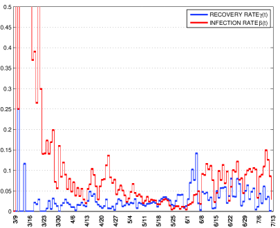
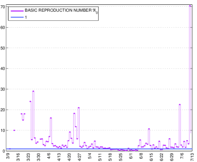
(a) the parameters $\beta(t)$ and $\gamma(t)$		(b) the basic reproduction number $\Re_{0}(t)$

Figure 2. Calculated values of SEIR model’s parameters and basic reproduction number for Bulgaria.

To verify TD-SEIR model (6) we solve recurrent sequence of initial problems (14) with obtained values $\beta_{k}$ and $\gamma_{k}$ ($\omega_{k}$ are fixed) for parameters. On the Figure 3 are shown the real data for active cases $A_{k}$ and Recovered individuals $R_{k}$ during the considered period, and the models curves, obtained using the calculated values $X_{k}(t_{k})+Y_{k}(t_{k})$ (for active cases) and $Z_{k}(t_{k})$ (for recovered individuals). We observe very good agreement between the calculated and the real data. All numerical simulations were performed using Matlab developed by MathWorks [26].

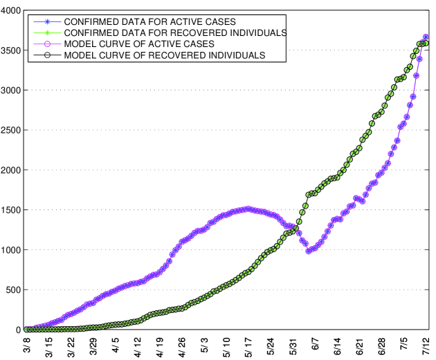
Figure 3. Confirmed data and SEIR model’s curves for Bulgaria.

We perform three sets of numerical experiments, related to predicting a 14-day-time-frame in the future, based on the available official data for Bulgaria up to the first day of the time frame. Those time frames are: April 20 – May 03, June 29 – July 12, and July 13 – July 26, respectively. The first time frame is related to the peak of the first wave of the virus. The second time frame is related to the last known date. The third time frame is a forecast for the future, thus we cannot compare the numerical results with official data.

To fix the notation, let the first day of the forecast period be denoted by $t_{K}$. Then, the last day of the forecast period will be $t_{K+13}$. We assume that the information, provided in the morning of every day $t_{k+1}$ is related to parameter values of the day $t_{k}$, $k=1,2,\dots,n-1$, e.g., the $79$ reported new cases on June 10 are considered as the $C_{k}$ value for June 9. We always solve the Cauchy problem (14) with initial data $\{S_{K-1},A_{K-1},I_{K-1},R_{K-1}\}$ and parameter $\omega=0.25,\beta_{K-2},\gamma_{K-2}$. The prediction of the parameters $\{\beta_{k}\}_{K-1}^{K+12}$ and $\{\gamma_{k}\}_{K-1}^{K+12}$ is performed on two levels. The first level uses the six ratios $\{\beta_{k}/\beta_{k+1}\}_{K-9}^{K-4}$, respectively $\{\gamma_{k}/\gamma_{k+1}\}_{K-9}^{K-4}$ from the week, before the time frame. The same ratios are used for both corresponding parameters from the first and second week of the forecast, e.g.,

$$\frac{\widetilde{\beta}_{K+5}}{\widetilde{\beta}_{K+6}}=\frac{\beta_{K-2}}{\widetilde{\beta}_{K-1}}=\frac{\beta_{K-9}}{\beta_{K-8}},\qquad\frac{\widetilde{\gamma}_{K+5}}{\widetilde{\gamma}_{K+6}}=\frac{\gamma_{K-2}}{\widetilde{\gamma}_{K-1}}=\frac{\gamma_{K-9}}{\gamma_{K-8}},$$

and analogously for the other five ratios. Note, that we denote by $\widetilde{\beta}_{k}$ and $\widetilde{\gamma}_{k}$ the predicted values of the parameters, using the proposed methodology, in order to distinguish them from the corresponding official ground-true data $\beta_{k}$ and $\gamma_{k}$, reported by the Bulgarian officials. We have tried several different approaches for optimal fitting of the parameter ratios, namely various convex combinations of the corresponding ratios for a longer time frame in the past (up to four weeks, see documented data in Table 1), but the best results were obtained by simple repetition of the ratios from the very last week, as described above. Possible explanations are related to the rapid changes in the government control measures and the continuous growth of licensed laboratories for PCR testing, which gradually increases the overall tested people every week.

Table 1. Documentation of the ratio $\beta_{k-2}/\beta_{k-1}$ on a weekly basis.

week	Mon/Tue	Tue/Wed	Wed/Thur	Thur/Fri	Fri/Sat	Sat/Sun
3/9 – 15	2.000	0.054	2.357	1.667	1.506	1.367
3/16 – 22	1.913	0.948	1.473	0.506	1.753	2.124
3/30 – 4/5	0.820	1.227	0.835	0.849	2.752	1.278
4/6 – 12	1.884	0.710	1.331	1.648	0.683	1.641
4/13 – 19	1.839	0.677	1.524	0.677	1.904	1.446
4/20 – 26	0.832	0.636	1.163	1.463	2.087	0.478
4/27 – 5/3	0.980	0.700	0.826	1.639	1.196	0.896
5/4 – 10	0.787	0.837	1.238	1.311	1.686	0.724
5/11 – 17	0.714	1.479	1.204	0.910	1.136	1.798
5/18 – 24	0.732	1.502	0.826	1.036	1.034	1.511
5/25 – 31	0.726	0.840	0.941	1.128	1.888	3.166
6/1 – 7	0.591	0.990	2.071	0.557	0.972	2.343
6/8 – 14	0.847	0.829	0.543	0.964	0.842	2.723
6/15 – 21	1.033	0.763	1.131	0.924	1.459	3.357
6/22 – 28	0.459	1.285	0.679	1.645	0.705	3.734
6/29 – 7/5	0.596	1.042	0.798	1.572	0.956	1.814
7/6 – 12	0.900	0.964	1.073	0.913	1.037	3.089

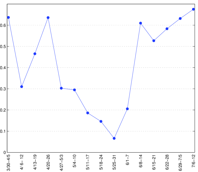
Figure 4. The accumulated data $\beta_{week_{i}}$

The second level is to approximate the accumulative week parameters $\{\beta_{week_{i}},\beta_{week_{i+1}}\}$, respectively $\{\gamma_{week_{i}},\gamma_{week_{i+1}}\}$ for the weeks: $week_{i}$ – the days between $t_{K}$ and $t_{K+6}$, and $week_{i+1}$ – the days between $t_{K+7}$ and $t_{K+13}$. For the first week, we have the obvious relation:

(15) $$\widetilde{\beta}_{week_{i}}:=\sum_{k=K-1}^{K+5}\widetilde{\beta}_{k},\qquad\widetilde{\gamma}_{week_{i}}:=\sum_{k=K-1}^{K+5}\widetilde{\gamma}_{k}.$$

For the second week, we fit $\beta_{week_{i+1}}$ and $\gamma_{week_{i+1}}$, using the available week information from several previous weeks. We used one fitting algorithm for the first time-frame and another fitting algorithm for the remaining two time-frames, due to particularities of the overall situation in Bulgaria (see Fig. 4). Further, once we predict $\widetilde{\beta}_{week_{i+1}}$ and $\widetilde{\gamma}_{week_{i+1}}$, together with the ratios $\{\widetilde{\beta}_{k}/\widetilde{\beta}_{k+1}\}_{K+6}^{K+11}$ $\{\widetilde{\beta}_{k}/\widetilde{\beta}_{k+1}\}_{K+6}^{K+11}$, we can straightforwardly invert (15) and derive $\{\widetilde{\beta}_{k}\}_{K+6}^{K+12}$, $\{\widetilde{\gamma}_{k}\}_{K+6}^{K+12}$. Finally, having all the necessary values $\{\widetilde{\beta}_{k}\}_{K-1}^{K+12}$ and $\{\widetilde{\gamma}_{k}\}_{K-1}^{K+12}$, we can solve the Cauchy problem TD-SEIR_k along the whole time period of interest.

For the first 14-days-time-frame April 20 – May 03, based on the data in Figure 4 we predicted $\widetilde{\beta}_{week_{i+1}}$ and $\widetilde{\gamma}_{week_{i+1}}$ via

$$\widetilde{\beta}_{week_{i+1}}=\widetilde{\beta}_{week_{i}}+\beta_{week_{i-2}}-\beta_{week_{i-3}},\qquad\widetilde{\gamma}_{week_{i+1}}=\frac{\widetilde{\gamma}_{week_{i}}+\gamma_{week_{i-1}}+\gamma_{week_{i-2}}+\gamma_{week_{i-3}}}{4}.$$

We used a parallelogram rule for the infection rate $\beta$ prediction, due to the strict government control measures at that time (facilities and parks closing, social distancing and travel restrictions, etc.). Thus, in general, the weekly infection rate was expected to monotonically decay towards zero. However, this was not the case for two consecutive weeks with linear growth of the parameter (April 13 – April 19 and April 20 – April 26), which was mainly due to the two big Orthodox holidays in Bulgaria: Palm Sunday (April 12) and Easter (April 19). The strict measures quickly inverted the monotonic behavior of $\beta$ and the weekly values for April 27 – May 3 were already in vicinity of those before the holidays (from April 6 – April 12). We used a simple averaging rule for the recovery rate $\gamma$ prediction, due to the early stage of the pandemic and the very long recovery period for infected patient. Therefore, practically most of the recovered individuals, counted within this period, were the deceased ones. This number behaved quite stably and did not oscillate much, meaning that it seemed natural to approximate it with a constant function.

The experimental comparison between the official data and our forecast is illustrated on the second row of Figure 5. We observe good agreement between the predicted and the real data. The number of actual cases (which is the biggest value and the most unpredictable one) is well fitted by our prediction. As expected, the longer the prediction period the larger the error, and our first week prediction is overall more accurate than the second week one. However, we managed to almost exactly capture the daily cases numbers on days 8, 9 and 13, which is quite a long-term forecast for the dynamics of the pandemic. The number of recovered individuals (as the smallest one among the three) is fitted the best.

Using TD-SEIR model (4) at the beginning of April 2020 we made forecast for COVID-19 spread among Bulgarian population. Let us mention that on 12.04.2020 we sent to the Bulgarian National Operating Center (NOC) a forecast for an expected peak the disease (of new cases per day) in Bulgaria on 26.04.2020. Later (at the end of April) the Bulgarian NOC reported a peak in the period 20.04 – 26.04. 2020.

For the second 14-days-time-frame June 29 – July 12, based on the data in Figure  4 we predicted $\widetilde{\beta}_{week_{i+1}}$ and $\widetilde{\gamma}_{week_{i+1}}$ via

$$\widetilde{\beta}_{week_{i+1}}=2\widetilde{\beta}_{week_{i}}-\beta_{week_{i-1}},\qquad\widetilde{\gamma}_{week_{i+1}}=\frac{\beta_{week_{i-5}}\widetilde{\gamma}_{week_{i}}+\beta_{week_{i-6}}\gamma_{week_{i-1}}}{2\beta_{week_{i-4}}}.$$

Note that, at the starting day $t_{K}$ of the first and second 14-days-time-frames the weekly behavior of the infection rate $\beta$ is quite similar. Indeed, we have had strong decrease in the value between weeks $i-3$ and $i-2$, followed by an increase of size at about half the decrease between weeks $i-2$ and $i-1$. During the first weeks of prediction, the $\beta_{week}$ behavior again remains similar: $\beta_{week_{i}}\approx\beta_{week_{i-3}}$ in both cases. The big difference appears in the second week of prediction. It was already mentioned about the strict government control measures during the first time frame. On the contrary, there were very mild government control measures during the second time frame – Shopping centers, parks, and even stadiums were open, high-school students were taking final exams and were allowed to organize prom balls, etc. As a result, the linear increase of $\beta_{week}$ holds true up to date. Therefore, we used linear fitting for the infection rate $\beta$ prediction. On the other hand, the percentage of healed patients among the recovered individuals drastically increased, meaning that simple averaging rule for the recovery rate $\gamma$ prediction was not adequate, any more. We conducted various numerical experiments and concluded, that the weekly behavior of the infection rate five weeks ago gives the most reliable information about the recovery rate during the current week, i.e., $\beta_{week_{i-5}}\gamma_{week_{i}}\approx const$. Therefore, we chose to fit this expression by a constant function. As input data, we used the information from the previous two values, since $\widetilde{\gamma}_{week_{i}}$ is again a prediction and not entirely reliable.

Active cases	Daily cases	Recovered individuals

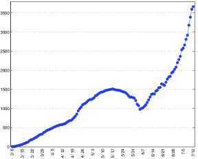
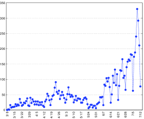
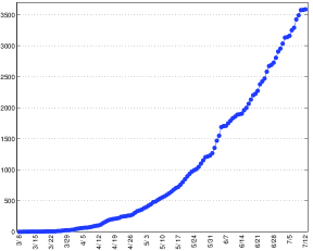
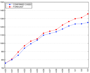
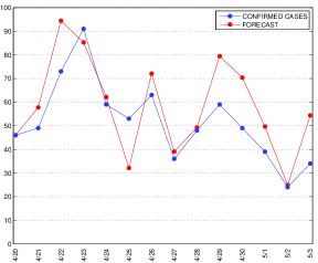
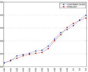
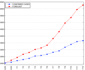
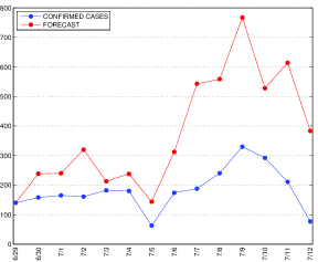
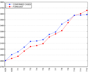
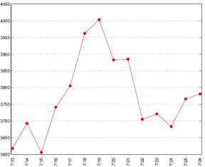
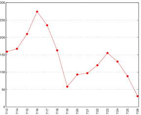
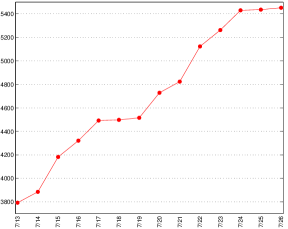
Figure 5. The three forecasts. Row 1: Complete data from the beginning of the pandemia until today. Row 2: First time period: 4/20 – 5/3. Row 3: Second time period: 6/29 – 7/12. Row 4: Third time period: 7/13 – 7/26. Official data is in blue, the predicted data is in red.

The experimental comparison between the official data and our forecast for the second time frame is illustrated on the third row of Figure 5. We observe an agreement between the predicted and the real data during the first week of the time frame, but not so much during the second one. As in the first forecast, the number of predicted active cases is always larger than the officially documented one, but the daily differences between the two plots are significantly larger than before. Apart from modeling obstructions, this behavior could also be explained with the decreased percentage of critical cases and the decreased average age of infected people. As a result, not all infected people test themselves and the official data could be significantly lower than reality. The same behavior is observed for the number of daily cases. The number of recovered individuals is fitted well.

Table 2. Relative errors of the prediction.

Compartment	First time period				Second time period
	$\ell_{2}$		$\ell_{\infty}$		$\ell_{2}$		$\ell_{\infty}$
	Week 1	Week 2	Week 1	Week 2	Week 1	Week 2	Week 1	Week 2
Active cases	0.026	0.052	0.036	0.083	0.159	0.564	0.214	0.711
Daily cases	0.197	0.333	0.235	0.362	0.537	1.428	0.873	1.325
Recovered	0.026	0.023	0.035	0.027	0.022	0.016	0.028	0.031

In order to analyze the accuracy of the proposed prediction methodology, the relative weekly-based errors for the compartments “Active cases” $\{A_{k}\}_{K}^{K+13}$, “Daily cases” $\{D_{k}:=A_{k}-A_{k-1}\}_{K}^{K+13}$, and “Recovered individuals” $\{R_{k}\}_{K}^{K+13}$ for both the first and the second 14-days-time-frames are documented in Table 2. Two different norms have been used - the $\ell_{2}$ one and the sup-norm $\ell_{\infty}$, i.e.,

$$Err_{A}(\ell_{2},week_{i}):=\frac{\|\widetilde{A}_{week_{i}}-A_{week_{i}}\|_{2}}{\|A_{week_{i}}\|_{2}},\qquad Err_{A}(\ell_{\infty},week_{i}):=\frac{\|\widetilde{A}_{week_{i}}-A_{week_{i}}\|_{\infty}}{\|A_{week_{i}}\|_{\infty}},$$

for the active cases and analogously for the other compartments. We observe good agreement between the corresponding error margins of the two norms, which suggests robustness of the proposed model with respect to the norm choice within the $\{\ell_{p}\}$ family. Further, in agreement with Fig. 5, we observe stable error behavior for the Recovered individuals, independent on the time period and the week of the period. For the remaining two compartments, we confirm that the second week prediction (days $\{t_{k}\}_{K+7}^{K+13}$) of each time period is less reliable than the first week prediction (days $\{t_{k}\}_{K}^{K+6}$) and that in the presence of strict government control measures our predictions are more accurate. Finally, we observe that the number of daily cases is the hardest one to predict, which is expected due to the lower values of that number and its day-by-day fluctuations.

For the third 14-days-time-frame July 13 – July 26 we apply the same setup as for the second time frame, as they are consecutive ones and nothing changed much in between. Here, we do not have official data to compare with, since this time period is in the future with respect to July 12. The forecast can be seen on the forth row of Figure 5.

4. Conclusions

In this paper, we applied a time-depended inverse SEIR model for daily adjustment of the infection rate $\beta(t_{k})$ and the recovery rate $\gamma(t_{k})$, based on a priori known information about the number of susceptible individuals $S(t_{k})$, the number of the active cases $A(t_{k})$, and the number of recovered individuals $R(t_{k})$. The problem becomes well-posed, if the latent rate $\omega(t_{k})$ and the number of infectious individuals $I(t_{k})$ is also given. For the former, we assume it to be a constant $\omega=1/T_{e}$, where the average incubation period in Europe $T_{e}=4$ is used. For the latter, we assume that $I(t_{0})=A(t_{0})$, i.e., all registered active cases at day one of the pandemic were infectious, and further compute $I(t_{k})$, based on all the data from day $t_{k-1}$.

Next, we developed a difference scheme for solving the discretized direct Cauchy problem that computes $S(t_{k})$, $A(t_{k})$, $I(t_{k})$, and $R(t_{k})$, based on $\beta(t_{k-1})$, $\gamma(t_{k-1})$, and $\omega(t_{k-1})$. Assuming, once again, that $\omega(t_{k})$ is constant, we developed a strategy for mid-time-term prediction of all compartments of the host population. The strategy takes into account the level of the government control measures, the new cases/tests dependency on the day of the week, and the length of the healing process. Three sets of numerical tests related to predicting a 14-day-time-frame, based on the available official data for Bulgaria up to the first day of the time frame were conducted. It was observed that in all our experiments the number of recovered individuals was well approximated along the whole time period. The numbers of active and daily cases were well approximated during the first week of the time period, but in the case of weak government control measures and lack of social distancing, the predicted values for the second week significantly exceeded the officially reported ones. A potential explanation is that the truth is somewhere in between, as there are infected people with mild or no symptoms, that do not test themselves, thus, do not appear in the governmental statistics. On the other hand, during strict government control measures with compulsory social distancing, the numbers of active and daily cases can be well approximated throughout the second week, as well.

5. Acknowledgments

The work of N. Popivanov and Ts. Hristov was partially supported by the Sofia University under Grant 80-10-112/2020 and 80-10-122/2020. The work of S. Margenov and S. Harizanov was partially supported by the National Scientific Program "Information and Communication Technologies for a Single Digital Market in Science, Education and Security (ICTinSES)", contract No DO1–205/23.11.2018, financed by the Ministry of Education and Science in Bulgaria.

References

- [1] M. Touma, COVID-19: molecular diagnostics overview, Journal of molecular medicine, 98, 947–954 (2020), https://doi.org/10.1007/s00109-020-01931-w
- [2] F. Zhou, T. Yu, R. Du, G. Fan, Y. Liu, Z. Liu, et al., Clinical course and risk factors for mortality of adult inpatients with COVID-19 in Wuhan, China: a retrospective cohort study, Lancet, 395(10229), 1054–1062 (2020), https://doi.org/10.1016/S0140-6736(20)30566-3
- [3] Y. Wang, Y. wang, Y. Chen, Q. Qin, Unique epidemiological and clinical features of the emerging 2019 novel coronavirus pneumonia (COVID-19) implicate special control measures, Journal of medical virology, 92(6), 568–576 (2020), https://doi.org/10.1002/jmv.25748
- [4] The Chris Murray COVID-19 forecasting model, http://www.healthdata.org/acting-data/our-covid-19-forecasting-model-otherwise-known-chris-murray-model
- [5] Gabriel Goh, Epidemic calculator, http://gabgoh.github.io/COVID/
- [6] N. Imai, I. Dorigatti, A. Cori, C. Donnelly, S. Riley, N. Ferguson, Report 2: Estimating the potential total number of novel Coronavirus cases in Wuhan City, China, 2020 Medical Research Council (MRC), http://hdl.handle.net/10044/1/77150
- [7] R. Verity at al., Estimates of the severity of coronavirus disease 2019: a model-based analysis. Lancet Infect Dis., 1–9 (2020), https://doi.org/10.1016/S1473-3099(20)30243-7
- [8] Y. Fang, Y. Nie, M. Penny, Transmission dynamics of the COVID-19 outbreak and effectiveness of government interventions: A data-driven analysis, J. Med. Virol., 1–15 (2020), https://doi.org/10.1002/jmv.25750
- [9] M. Liu, J. Cao, J. Liang, M. Chen, Epidemic-logistics Modeling: A New Perspective on Operations Research, Springer, 2020, https://doi.org/10.1007/978-981-13-9353-2
- [10] Pauline van den Driessche, Reproduction numbers of infectious disease models, Infect Dis Model., Vol. 2(3), 288 – 303 (2017), https://doi.org/10.1016/j.idm.2017.06.002
- [11] J. Carcione, J. Santos, C. Bagaini, J. Ba, A Simulation of a COVID-19 Epidemic Based on a Deterministic SEIR Model, Frontiers in Public Health, Vol. 8(230), 1–13 (2020), https://doi.org/10.3389/fpubh.2020.00230
- [12] W. Kermack, A. McKendrick, A contribution to the mathematical theory of pandemics. Proc R Soc Lond, Series A., 115(772): 700–721 (1927).
- [13] P. White, 5 - Mathematical Models in Infectious Disease Epidemiology, Infectious Diseases (Fourth Edition), Elsevier, 49-53.e1 (2017), https://doi.org/10.1016/B978-0-7020-6285-8.00005-8
- [14] J. Ponciano, M. Capistran, First Principles Modeling of Nonlinear Incidence Rates in Seasonal Epidemics, PLOS Computational Biology, 7(2): e1001079 (2011), https://doi.org/10.1371/journal.pcbi.1001079
- [15] Z. Chladna, J. Kopfova, D. Rachinskii, S. Rouf, Global dynamics of SIR model with switched transmission rate, J. Math. Biol., 80, 1209–1233 (2020), https://doi.org/10.1007/s00285-019-01460-2
- [16] X. Liu, P. Stechlinski, Infectious disease models with time-varying parameters and general nonlinear incidence rate, Applied Mathematical Modelling, 36(5), 1974–1994 (2012), https://doi.org/10.1016/j.apm.2011.08.019
- [17] D. Brockmann, V. David, A.M. Gallardo, Human Mobility and Spatial Disease Dynamics, Open-Access Journal for the Basic Principles of Diffusion Theory, Experiment and Application, 11 (2), 1–27 (2009).
- [18] Y. Jiang, R. Kassem, G. York, M. Junge, R. Durrett, SIR epidemics on evolving graphs, arXiv:1901.06568, 1–24 (2019), https://arxiv.org/abs/1901.06568
- [19] N. Liu, J. Fang, W. Deng, J. Sun, Stability analysis of a fractional-order SIS model on complex networks with linear treatment function, Advances in Difference Equations 327, 1–10 (2019), https://doi.org/10.1186/s13662-019-2234-x
- [20] B. Takacs, R. Horvath, I. Farag o, Space dependent models for studying the spread of some diseases, Computers & Mathematics with Applications, 80(2), 395–404 (2020), https://doi.org/10.1016/j.camwa.2019.07.001
- [21] Institute for Health Metrics and Evaluation (IHME), http://www.healthdata.org/
- [22] Y-C. Chen, P-E Lu, T-H Liu, A Time-dependent SIR model for COVID-19 with Undetectable Infected Persons, arXiv:2003.00122. 11 Apr 2020; 1–16 (2020), https://arxiv.org/abs/2003.00122
- [23] O. Kounchev, G. Simeonov, Z. Kuncheva, The TVBG-SEIR spline model for analysis of COVID-19 spread, and a Tool for prediction scenarios, arXiv:2004.11338 [math.NA]. 1–21 (2020), https://arxiv.org/ftp/arxiv/papers/2004/2004.11338.pdf
- [24] J. Ma, Estimating epidemic exponential growth rate and basic reproduction number, Infectious Disease Modelling, Vol. 5, 129–141(2020), https://doi.org/10.1016/j.idm.2019.12.009
- [25] M. Böhmer et al., Investigation of a COVID-19 outbreak in Germany resulting from a single travel-associated primary case: a case series, The Lancet Infectious Diseases, 1–9 (2020), https://doi.org/10.1016/S1473-3099(20)30314-5
- [26] The MathWorks, Inc., MATLAB, https://www.mathworks.com/products/matlab.html