Taming the fixed-node error in diffusion Monte Carlo via range separation

Abstract

By combining density-functional theory (DFT) and wave function theory (WFT) via the range separation (RS) of the interelectronic Coulomb operator, we obtain accurate fixed-node diffusion Monte Carlo (FN-DMC) energies with compact multi-determinant trial wave functions. In particular, we combine here short-range exchange-correlation functionals with a flavor of selected configuration interaction (SCI) known as configuration interaction using a perturbative selection made iteratively (CIPSI), a scheme that we label RS-DFT-CIPSI. One of the take-home messages of the present study is that RS-DFT-CIPSI trial wave functions yield lower fixed-node energies with more compact multi-determinant expansions than CIPSI, especially for small basis sets. Indeed, as the CIPSI component of RS-DFT-CIPSI is relieved from describing the short-range part of the correlation hole around the electron-electron coalescence points, the number of determinants in the trial wave function required to reach a given accuracy is significantly reduced as compared to a conventional CIPSI calculation. Importantly, by performing various numerical experiments, we evidence that the RS-DFT scheme essentially plays the role of a simple Jastrow factor by mimicking short-range correlation effects, hence avoiding the burden of performing a stochastic optimization. Considering the 55 atomization energies of the Gaussian-1 benchmark set of molecules, we show that using a fixed value of $\mu=0.5$ bohr^-1 provides effective error cancellations as well as compact trial wave functions, making the present method a good candidate for the accurate description of large chemical systems.

I Introduction

Solving the Schrödinger equation for the ground state of atoms and molecules is a complex task that has kept theoretical and computational chemists busy for almost a hundred years now. Schrödinger (1926) In order to achieve this formidable endeavor, various strategies have been carefully designed and efficiently implemented in various quantum chemistry software packages.

I.1 Wave function-based methods

One of these strategies consists in relying on wave function theory Pople (1999) (WFT) and, in particular, on the full configuration interaction (FCI) method. However, FCI delivers only the exact solution of the Schrödinger equation within a finite basis (FB) of one-electron functions, the FB-FCI energy being an upper bound to the exact energy in accordance with the variational principle. The FB-FCI wave function and its corresponding energy form the eigenpair of an approximate Hamiltonian defined as the projection of the exact Hamiltonian onto the finite many-electron basis of all possible Slater determinants generated within this finite one-electron basis. The FB-FCI wave function can then be interpreted as a constrained solution of the true Hamiltonian forced to span the restricted space provided by the finite one-electron basis. In the complete basis set (CBS) limit, the constraint is lifted and the exact energy and wave function are recovered. Hence, the accuracy of a FB-FCI calculation can be systematically improved by increasing the size of the one-electron basis set. Nevertheless, the exponential growth of its computational cost with the number of electrons and with the basis set size is prohibitive for most chemical systems.

In recent years, the introduction of new algorithms White (1992); Booth, Thom, and Alavi (2009); Thom (2010); Xu, Uejima, and Ten-no (2018); Motta and Zhang (2018); Deustua et al. (2018); Eriksen and Gauss (2018, 2019); Ghanem, Lozovoi, and Alavi (2019) and the revival Abrams and Sherrill (2005); Bytautas and Ruedenberg (2009); Roth (2009); Giner, Scemama, and Caffarel (2013); Knowles (2015); Holmes, Changlani, and Umrigar (2016); Holmes, Umrigar, and Sharma (2017); Sharma et al. (2017); Evangelista (2014); Liu and Hoffmann (2016); Tubman et al. (2016, 2020); Per and Cleland (2017); Zimmerman (2017); Ohtsuka and ya Hasegawa (2017); Garniron et al. (2018) of selected configuration interaction (SCI) methods Bender and Davidson (1969); Huron, Malrieu, and Rancurel (1973); Buenker and Peyerimhoff (1974) significantly expanded the range of applicability of this family of methods. Importantly, one can now routinely compute the ground- and excited-state energies of small- and medium-sized molecular systems with near-FCI accuracy. Booth and Alavi (2010); Cleland, Booth, and Alavi (2010); Daday et al. (2012); Motta et al. (2017); Chien et al. (2018); Loos et al. (2018, 2019a, 2020a, 2020b); Williams et al. (2020); Eriksen et al. (2020) However, although the prefactor is reduced, the overall computational scaling remains exponential unless some bias is introduced leading to a loss of size consistency. Evangelisti, Daudey, and Malrieu (1983); Cleland, Booth, and Alavi (2010); Ten-no (2017); Ghanem, Lozovoi, and Alavi (2019)

I.2 Density-based methods

Another route to solve the Schrödinger equation is density-functional theory (DFT). Hohenberg and Kohn (1964); Kohn (1999) Present-day DFT calculations are almost exclusively done within the so-called Kohn-Sham (KS) formalism, Kohn and Sham (1965) which transfers the complexity of the many-body problem to the universal and yet unknown exchange-correlation (xc) functional thanks to a judicious mapping between a non-interacting reference system and its interacting analog which both have the same one-electron density. KS-DFT Hohenberg and Kohn (1964); Kohn and Sham (1965) is now the workhorse of electronic structure calculations for atoms, molecules and solids thanks to its very favorable accuracy/cost ratio. Parr and Yang (1989) As compared to WFT, DFT has the indisputable advantage of converging much faster with respect to the size of the basis set. Franck et al. (2015); Giner et al. (2018); Loos et al. (2019b); Giner et al. (2020) However, unlike WFT where, for example, many-body perturbation theory provides a precious tool to go toward the exact wave function, there is no systematic way to improve approximate xc functionals toward the exact functional. Therefore, one faces, in practice, the unsettling choice of the approximate xc functional. Becke (2014) Moreover, because of the approximate nature of the xc functional, although the resolution of the KS equations is variational, the resulting KS energy does not have such property.

I.3 Stochastic methods

Diffusion Monte Carlo (DMC) belongs to the family of stochastic methods known as quantum Monte Carlo (QMC) and is yet another numerical scheme to obtain the exact solution of the Schrödinger equation with a different twist. Foulkes et al. (2001); Austin, Zubarev, and Lester (2012); Needs et al. (2020) In DMC, the solution is imposed to have the same nodes (or zeroes) as a given (approximate) antisymmetric trial wave function. Reynolds et al. (1982); Ceperley (1991) Within this so-called fixed-node (FN) approximation, the FN-DMC energy associated with a given trial wave function is an upper bound to the exact energy, and the latter is recovered only when the nodes of the trial wave function coincide with the nodes of the exact wave function. The trial wave function, which can be single- or multi-determinantal in nature depending on the type of correlation at play and the target accuracy, is the key ingredient dictating, via the quality of its nodal surface, the accuracy of the resulting energy and properties.

The polynomial scaling of its computational cost with respect to the number of electrons and with the size of the trial wave function makes the FN-DMC method particularly attractive. This favorable scaling, its very low memory requirements and its adequacy with massively parallel architectures make it a serious alternative for high-accuracy simulations of large systems. Nakano et al. (2020); Scemama et al. (2013); Needs et al. (2020); Kim et al. (2018); Kent et al. (2020) In addition, the total energies obtained are usually far below those obtained with the FCI method in computationally tractable basis sets because the constraints imposed by the fixed-node approximation are less severe than the constraints imposed by the finite-basis approximation. However, because it is not possible to minimize directly the FN-DMC energy with respect to the linear and non-linear parameters of the trial wave function, the fixed-node approximation is much more difficult to control than the finite-basis approximation, especially to compute energy differences. The conventional approach consists in multiplying the determinantal part of the trial wave function by a positive function, the Jastrow factor, which main assignment is to take into account the bulk of the dynamical electron correlation and reduce the statistical fluctuations without altering the location of the nodes. The determinantal part of the trial wave function is then stochastically re-optimized within variational Monte Carlo (VMC) in the presence of the Jastrow factor (which can also be simultaneously optimized) and the nodal surface is expected to be improved. Umrigar and Filippi (2005); Scemama and Filippi (2006); Umrigar et al. (2007); Toulouse and Umrigar (2007, 2008) Using this technique, it has been shown that the chemical accuracy could be reached within FN-DMC.Petruzielo, Toulouse, and Umrigar (2012)

I.4 Single-determinant trial wave functions

The qualitative picture of the electronic structure of weakly correlated systems, such as organic molecules near their equilibrium geometry, is usually well represented with a single Slater determinant. This feature is in part responsible for the success of DFT and coupled cluster (CC) theory. Likewise, DMC with a single-determinant trial wave function can be used as a single-reference post-Hartree-Fock method for weakly correlated systems, with an accuracy comparable to CCSD(T), Dubecký et al. (2014); Grossman (2002) the gold standard of WFT for ground state energies. Cizek ; Purvis III and Bartlett (1982) In single-determinant DMC calculations, the only degree of freedom available to reduce the fixed-node error are the molecular orbitals with which the Slater determinant is built. Different molecular orbitals can be chosen: Hartree-Fock (HF), Kohn-Sham (KS), natural orbitals (NOs) of a correlated wave function, or orbitals optimized in the presence of a Jastrow factor. Nodal surfaces obtained with a KS determinant are in general better than those obtained with a HF determinant,Per, Walker, and Russo (2012) and of comparable quality to those obtained with a Slater determinant built with NOs.Wang, Zhou, and Wang (2019) Orbitals obtained in the presence of a Jastrow factor are generally superior to KS orbitals.Filippi and Fahy (2000); Scemama and Filippi (2006); Haghighi Mood and Lüchow (2017); Ludovicy, Mood, and Lüchow (2019)

The description of electron correlation within DFT is very different from correlated methods such as FCI or CC. As mentioned above, within KS-DFT, one solves a mean-field problem with a modified potential incorporating the effects of electron correlation while maintaining the exact ground state density, whereas in correlated methods the real Hamiltonian is used and the electron-electron interaction is explicitly considered. Nevertheless, as the orbitals are one-electron functions, the procedure of orbital optimization in the presence of a Jastrow factor can be interpreted as a self-consistent field procedure with an effective Hamiltonian,Filippi and Fahy (2000) similarly to DFT. So KS-DFT can be viewed as a very cheap way of introducing the effect of correlation in the orbital coefficients dictating the location of the nodes of a single Slater determinant. Yet, even when employing the exact xc potential in a complete basis set, a fixed-node error necessarily remains because the single-determinant ansätz does not have enough flexibility for describing the nodal surface of the exact correlated wave function for a generic many-electron system. Ceperley (1991); Bressanini (2012); Loos and Bressanini (2015) If one wants to recover the exact energy, a multi-determinant parameterization of the wave functions must be considered.

I.5 Multi-determinant trial wave functions

The single-determinant trial wave function approach obviously fails in the presence of strong correlation, like in transition metal complexes, low-spin open-shell systems, and covalent bond breaking situations which cannot be qualitatively described by a single electronic configuration. In such cases or when very high accuracy is required, a viable alternative is to consider the FN-DMC method as a “post-FCI” method. A multi-determinant trial wave function is then produced by approaching FCI with a SCI method such as configuration interaction using a perturbative selection made iteratively (CIPSI). Giner, Scemama, and Caffarel (2013, 2015); Caf (2016) When the basis set is enlarged, the trial wave function gets closer to the exact wave function, so we expect the nodal surface to be improved.Caffarel et al. (2016) Note that, as discussed in Ref. Caf, 2016, there is no mathematical guarantee that increasing the size of the one-electron basis lowers the FN-DMC energy, because the variational principle does not explicitly optimize the nodal surface, nor the FN-DMC energy. However, in all applications performed so far, Giner, Scemama, and Caffarel (2013); Scemama et al. (2014, 2016); Giner, Scemama, and Caffarel (2015); Caffarel et al. (2016); Scemama et al. (2018a, b, 2019) a systematic decrease of the FN-DMC energy has been observed whenever the SCI trial wave function is improved variationally upon enlargement of the basis set.

The technique relying on CIPSI multi-determinant trial wave functions described above has the advantage of using near-FCI quality nodes in a given basis set, which is perfectly well defined and therefore makes the calculations systematically improvable and reproducible in a black-box way without needing any QMC expertise. Nevertheless, this procedure cannot be applied to large systems because of the exponential growth of the number of Slater determinants in the trial wave function. Extrapolation techniques have been employed to estimate the FN-DMC energies obtained with FCI wave functions,Scemama et al. (2018a, b, 2019) and other authors have used a combination of the two approaches where highly truncated CIPSI trial wave functions are stochastically re-optimized in VMC under the presence of a Jastrow factor to keep the number of determinants small,Giner, Assaraf, and Toulouse (2016) and where the consistency between the different wave functions is kept by imposing a constant energy difference between the estimated FCI energy and the variational energy of the SCI wave function.Dash et al. (2018, 2019) Nevertheless, finding a robust protocol to obtain high accuracy calculations which can be reproduced systematically and applicable to large systems with a multi-configurational character is still an active field of research. The present paper falls within this context.

The central idea of the present work, and the launch pad for the remainder of this study, is that one can combine the various strengths of WFT, DFT, and QMC in order to create a new hybrid method with more attractive features and higher accuracy. In particular, we show here that one can combine CIPSI and KS-DFT via the range separation (RS) of the interelectronic Coulomb operator Savin (1996a); Toulouse, Colonna, and Savin (2004) — a scheme that we label RS-DFT-CIPSI in the following — to obtain accurate FN-DMC energies with compact multi-determinant trial wave functions. An important take-home message from the present study is that the RS-DFT scheme essentially plays the role of a simple Jastrow factor by mimicking short-range correlation effects. Thanks to this, RS-DFT-CIPSI multi-determinant trial wave functions yield lower fixed-node energies with more compact multi-determinant expansion than CIPSI, especially for small basis sets, and can be produced in a completely deterministic and systematic way, without the burden of the stochastic optimization.

The present manuscript is organized as follows. In Sec. II, we provide theoretical details about the CIPSI algorithm (Sec. II.1) and range-separated DFT (Sec. II.2). Computational details are reported in Sec. III. In Sec. IV, we discuss the influence of the range-separation parameter on the fixed-node error as well as the link between RS-DFT and Jastrow factors. Section V examines the performance of the present scheme for the atomization energies of the Gaussian-1 set of molecules. Finally, we draw our conclusion in Sec. VI. Unless otherwise stated, atomic units are used.

II Theory

II.1 The CIPSI algorithm

Beyond the single-determinant representation, the best multi-determinant wave function one can wish for — in a given basis set — is the FCI wave function. FCI is the ultimate goal of post-HF methods, and there exist several systematic improvements on the path from HF to FCI: i) increasing the maximum degree of excitation of CI methods (CISD, CISDT, CISDTQ, …), or ii) expanding the size of a complete active space (CAS) wave function until all the orbitals are in the active space. SCI methods take a shortcut between the HF determinant and the FCI wave function by increasing iteratively the number of determinants on which the wave function is expanded, selecting the determinants which are expected to contribute the most to the FCI wave function. At each iteration, the lowest eigenpair is extracted from the CI matrix expressed in the determinant subspace, and the FCI energy can be estimated by adding up to the variational energy a second-order perturbative correction (PT2), $E_{\text{PT2}}$. The magnitude of $E_{\text{PT2}}$ is a measure of the distance to the FCI energy and a diagnostic of the quality of the wave function. Within the CIPSI algorithm originally developed by Huron et al. in Ref. Huron, Malrieu, and Rancurel, 1973 and efficiently implemented in Quantum Package as described in Ref. Garniron et al., 2019, the PT2 correction is computed simultaneously to the determinant selection at no extra cost. $E_{\text{PT2}}$ is then the sole parameter of the CIPSI algorithm and is chosen to be its convergence criterion.

II.2 Range-separated DFT

Range-separated DFT (RS-DFT) was introduced in the seminal work of Savin. Savin (1996a); Toulouse, Colonna, and Savin (2004) In RS-DFT, the Coulomb operator entering the electron-electron repulsion is split into two pieces:

$$\frac{1}{r}=w_{\text{ee}}^{\text{sr},\mu}(r)+w_{\text{ee}}^{\text{lr},\mu}(r),$$ (1)

where

$$w_{\text{ee}}^{\text{sr},\mu}(r) =\frac{\operatorname{erfc}\quantity(\mu\,r)}{r}, w_{\text{ee}}^{\text{lr},\mu}(r) =\frac{\erf\quantity(\mu\,r)}{r}$$ (2)

are the singular short-range (sr) part and the non-singular long-range (lr) part, respectively, $\mu$ is the range-separation parameter which controls how rapidly the short-range part decays, $\erf(x)$ is the error function, and $\operatorname{erfc}(x)=1-\erf(x)$ is its complementary version.

The main idea behind RS-DFT is to treat the short-range part of the interaction using a density functional, and the long-range part within a WFT method like FCI in the present case. The parameter $\mu$ controls the range of the separation, and allows to go continuously from the KS Hamiltonian ($\mu=0$) to the FCI Hamiltonian ($\mu=\infty$).

To rigorously connect WFT and DFT, the universal Levy-Lieb density functional Levy (1979); Lieb (1983) is decomposed as

$$\mathcal{F}[n]=\mathcal{F}^{\text{lr},\mu}[n]+\bar{E}_{\text{Hxc}}^{\text{sr,}\mu}[n],$$ (3)

where $n$ is a one-electron density, $\mathcal{F}^{\text{lr},\mu}$ is a long-range universal density functional and $\bar{E}_{\text{Hxc}}^{\text{sr,}\mu}$ is the complementary short-range Hartree-exchange-correlation (Hxc) density functional. Savin (1996b); Toulouse, Colonna, and Savin (2004) The exact ground state energy can be therefore obtained as a minimization over a multi-determinant wave function as follows:

$$E_{0}=\min_{\Psi}\quantity{\matrixelement{\Psi}{\hat{T}+\hat{W}_{\text{{ee}}}^{\text{lr},\mu}+\hat{V}_{\text{ne}}}{\Psi}+\bar{E}^{\text{sr},\mu}_{\text{Hxc}}[n_{\Psi}]},$$ (4)

with $\hat{T}$ the kinetic energy operator, $\hat{W}_{\text{ee}}^{\text{lr},\mu}$ the long-range electron-electron interaction, $n_{\Psi}$ the one-electron density associated with $\Psi$, and $\hat{V}_{\text{ne}}$ the electron-nucleus potential. The minimizing multi-determinant wave function $\Psi^{\mu}$ can be determined by the self-consistent eigenvalue equation

$$\hat{H}^{\mu}[n_{\Psi^{\mu}}]\ket{\Psi^{\mu}}=\mathcal{E}^{\mu}\ket{\Psi^{\mu}},$$ (5)

with the long-range interacting Hamiltonian

$$\hat{H}^{\mu}[n_{\Psi^{\mu}}]=\hat{T}+\hat{W}_{\text{ee}}^{\text{lr},\mu}+\hat{V}_{\text{ne}}+\hat{\bar{V}}_{\text{Hxc}}^{\text{sr},\mu}[n_{\Psi^{\mu}}],$$ (6)

where $\hat{\bar{V}}_{\text{Hxc}}^{\text{sr},\mu}$ is the complementary short-range Hartree-exchange-correlation potential operator. Once $\Psi^{\mu}$ has been calculated, the electronic ground-state energy is obtained as

$$E_{0}=\matrixelement{\Psi^{\mu}}{\hat{T}+\hat{W}_{\text{{ee}}}^{\text{lr},\mu}+\hat{V}_{\text{ne}}}{\Psi^{\mu}}+\bar{E}^{\text{sr},\mu}_{\text{Hxc}}[n_{\Psi^{\mu}}].$$ (7)

Note that, for $\mu=0$, the long-range interaction vanishes, i.e., $w_{\text{ee}}^{\text{lr},\mu=0}(r)=0$, and thus RS-DFT reduces to standard KS-DFT and $\Psi^{\mu}$ is the KS determinant. For $\mu=\infty$, the long-range interaction becomes the standard Coulomb interaction, i.e., $w_{\text{ee}}^{\text{lr},\mu\to\infty}(r)=r^{-1}$, and thus RS-DFT reduces to standard WFT and $\Psi^{\mu}$ is the FCI wave function.

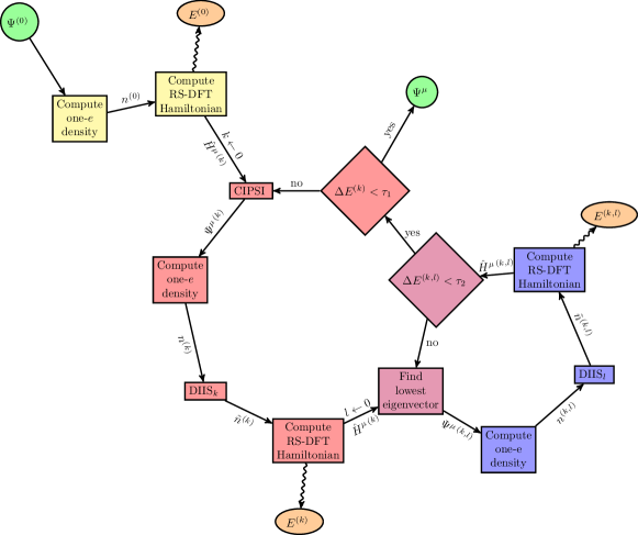
Figure 1: Algorithm showing the generation of the RS-DFT wave function $\Psi^{\mu}$ starting from $\Psi^{(0)}$. The outer (macro-iteration) and inner (micro-iteration) loops are represented in red and blue, respectively. The steps common to both loops are represented in purple. DIIS extrapolations of the one-electron density are introduced in both the outer and inner loops in order to speed up convergence of the self-consistent process.

Hence, range separation creates a continuous path connecting smoothly the KS determinant to the FCI wave function. Because the KS nodes are of higher quality than the HF nodes (see Sec. I.4), we expect that using wave functions built along this path will always provide reduced fixed-node errors compared to the path connecting HF to FCI which consists in increasing the number of determinants.

We follow the KS-to-FCI path by performing FCI calculations using the RS-DFT Hamiltonian with different values of $\mu$. Our algorithm, depicted in Fig. 1, starts with a single- or multi-determinant wave function $\Psi^{(0)}$ which can be obtained in many different ways depending on the system that one considers. One of the particularity of the present work is that we use the CIPSI algorithm to perform approximate FCI calculations with the RS-DFT Hamiltonian $\hat{H}^{\mu}$. Giner et al. (2018) This provides a multi-determinant trial wave function $\Psi^{\mu}$ that one can “feed” to DMC. In the outer (macro-iteration) loop (red), at the $k$th iteration, a CIPSI selection is performed to obtain $\Psi^{\mu\,(k)}$ with the RS-DFT Hamiltonian $\hat{H}^{\mu\,(k)}$ parameterized using the current one-electron density $n^{(k)}$. At each iteration, the number of determinants in $\Psi^{\mu\,(k)}$ increases. One exits the outer loop when the absolute energy difference between two successive macro-iterations $\Delta E^{(k)}$ is below a threshold $\tau_{1}$ that has been set to $10^{-3}$ $E_{h}$ in the present study and which is consistent with the CIPSI threshold (see Sec. III). An inner (micro-iteration) loop (blue) is introduced to accelerate the convergence of the self-consistent calculation, in which the set of determinants in $\Psi^{\mu\,(k,l)}$ is kept fixed, and only the diagonalization of $\hat{H}^{\mu\,(k,l)}$ is performed iteratively with the updated density $n^{(k,l)}$. The inner loop is exited when the absolute energy difference between two successive micro-iterations $\Delta E^{(k,l)}$ is below a threshold $\tau_{2}$ that has been here set to $10^{-2}\times\tau_{1}$. The convergence of the algorithm was further improved by introducing a direct inversion in the iterative subspace (DIIS) step to extrapolate the one-electron density both in the outer and inner loops. Pulay (1980, 1982) We emphasize that any range-separated post-HF method can be implemented using this scheme by just replacing the CIPSI step by the post-HF method of interest. Note that, thanks to the self-consistent nature of the algorithm, the final trial wave function $\Psi^{\mu}$ is independent of the starting wave function $\Psi^{(0)}$.

III Computational details

All reference data (geometries, atomization energies, zero-point energy, etc) were taken from the NIST computational chemistry comparison and benchmark database (CCCBDB).Johnson (2002) In the reference atomization energies, the zero-point vibrational energy was removed from the experimental atomization energies.

All calculations have been performed using Burkatzki-Filippi-Dolg (BFD) pseudopotentials Burkatzki, Filippi, and Dolg (2007, 2008) with the associated double-, triple-, and quadruple-$\zeta$ basis sets (V$X$Z-BFD). The small-core BFD pseudopotentials include scalar relativistic effects. Coupled cluster with singles, doubles, and perturbative triples [CCSD(T)] Scuseria, Janssen, and III (1988); Scuseria and III (1989) and KS-DFT energies have been computed with Gaussian09,Frisch et al. (2016) using the unrestricted formalism for open-shell systems.

The CIPSI calculations have been performed with Quantum Package.Garniron et al. (2019); Scemama et al. (2020) We consider the short-range version of the local-density approximation (LDA)Savin (1996a); Toulouse, Savin, and Flad (2004) and Perdew-Burke-Ernzerhof (PBE) Perdew, Burke, and Ernzerhof (1996) xc functionals defined in Ref. Goll et al., 2006 (see also Refs. Toulouse, Colonna, and Savin, 2005; Goll, Werner, and Stoll, 2005) that we label srLDA and srPBE respectively in the following. In this work, we target chemical accuracy, so the convergence criterion for stopping the CIPSI calculations has been set to $E_{\text{PT2}}<10^{-3}$ $E_{h}$ or $N_{\text{det}}>10^{7}$. All the wave functions are eigenfunctions of the $\hat{S}^{2}$ spin operator, as described in Ref. Applencourt, Gasperich, and Scemama, 2018.

QMC calculations have been performed with QMC=Chem,Scemama et al. (2013) in the determinant localization approximation (DLA),Zen et al. (2019) where only the determinantal component of the trial wave function is present in the expression of the wave function on which the pseudopotential is localized. Hence, in the DLA, the fixed-node energy is independent of the Jastrow factor, as in all-electron calculations. Simple Jastrow factors were used to reduce the fluctuations of the local energy (see Sec. IV.2 for their explicit expression). The FN-DMC simulations are performed with all-electron moves using the stochastic reconfiguration algorithm developed by Assaraf et al. Assaraf, Caffarel, and Khelif (2000) with a time step of $5\times 10^{-4}$ a.u., independent populations of 100 walkers and a projecting time of $1$ a.u. With such parameters, both the time-step error and the bias due to the finite projecting time are smaller than the error bars.

All the data related to the present study (geometries, basis sets, total energies, etc) can be found in the supplementary material.

IV Influence of the range-separation parameter on the fixed-node error

Table 1: FN-DMC energy $E_{\text{FN-DMC}}$ (in $E_{h}$) and number of determinants $N_{\text{det}}$ in H2O for various trial wave functions $\Psi^{\mu}$ obtained with the srPBE density functional.

	VDZ-BFD		VTZ-BFD
$\mu$	$N_{\text{det}}$	$E_{\text{FN-DMC}}$	$N_{\text{det}}$	$E_{\text{FN-DMC}}$
$0.00$	$11$	$-17.253\,59(6)$	$23$	$-17.256\,74(7)$
$0.20$	$23$	$-17.253\,73(7)$	$23$	$-17.256\,73(8)$
$0.30$	$53$	$-17.253\,4(2)$	$219$	$-17.253\,7(5)$
$0.50$	$1\,442$	$-17.253\,9(2)$	$16\,99$	$-17.257\,7(2)$
$0.75$	$3\,213$	$-17.255\,1(2)$	$13\,362$	$-17.258\,4(3)$
$1.00$	$6\,743$	$-17.256\,6(2)$	$256\,73$	$-17.261\,0(2)$
$1.75$	$54\,540$	$-17.259\,5(3)$	$207\,475$	$-17.263\,5(2)$
$2.50$	$51\,691$	$-17.259\,4(3)$	$858\,123$	$-17.264\,3(3)$
$3.80$	$103\,059$	$-17.258\,7(3)$	$1\,621\,513$	$-17.263\,7(3)$
$5.70$	$102\,599$	$-17.257\,7(3)$	$1\,629\,655$	$-17.263\,2(3)$
$8.50$	$101\,803$	$-17.257\,3(3)$	$1\,643\,301$	$-17.263\,3(4)$
$\infty$	$200\,521$	$-17.256\,8(6)$	$1\,631\,982$	$-17.263\,9(3)$

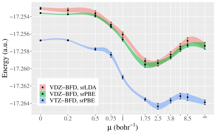
Figure 2: FN-DMC energy of H2O as a function of $\mu$ for various trial wave functions $\Psi^{\mu}$ generated at different levels of theory. The raw data can be found in the supplementary material.

The first question we would like to address is the quality of the nodes of the wave function $\Psi^{\mu}$ obtained for intermediate values of the range separation parameter (i.e., $0<\mu<+\infty$). For this purpose, we consider a weakly correlated molecular system, namely the water molecule at its experimental geometry. Caffarel et al. (2016) We then generate trial wave functions $\Psi^{\mu}$ for multiple values of $\mu$, and compute the associated FN-DMC energy keeping fixed all the parameters impacting the nodal surface, such as the CI coefficients and the molecular orbitals.

IV.1 Fixed-node energy of RS-DFT-CIPSI trial wave functions

From Table 1 and Fig. 2, where we report the fixed-node energy of H2O as a function of $\mu$ for various short-range density functionals and basis sets, one can clearly observe that relying on FCI trial wave functions ($\mu=\infty$) give FN-DMC energies lower than the energies obtained with a single KS determinant ($\mu=0$): a lowering of $3.2\pm 0.6$ m$E_{h}$ at the double-$\zeta$ level and $7.2\pm 0.3$ m$E_{h}$ at the triple-$\zeta$ level are obtained with the srPBE functional. Coming now to the nodes of the trial wave function $\Psi^{\mu}$ with intermediate values of $\mu$, Fig. 2 shows that a smooth behavior is obtained: starting from $\mu=0$ (i.e., the KS determinant), the FN-DMC error is reduced continuously until it reaches a minimum for an optimal value of $\mu$ (which is obviously basis set and functional dependent), and then the FN-DMC error raises until it reaches the $\mu=\infty$ limit (i.e., the FCI wave function). For instance, with respect to the fixed-node energy associated with the RS-DFT-CIPSI(srPBE/VDZ-BFD) trial wave function at $\mu=\infty$, one can obtain a lowering of the FN-DMC energy of $2.6\pm 0.7$ m$E_{h}$ with an optimal value of $\mu=1.75$ bohr^-1. This lowering in FN-DMC energy is to be compared with the $3.2\pm 0.7$ m$E_{h}$ gain in FN-DMC energy between the KS wave function ($\mu=0$) and the FCI wave function ($\mu=\infty$). When the basis set is improved, the gain in FN-DMC energy with respect to the FCI trial wave function is reduced, and the optimal value of $\mu$ is slightly shifted towards large $\mu$ as expected. Last but not least, the nodes of the wave functions $\Psi^{\mu}$ obtained with the srLDA functional give very similar FN-DMC energies with respect to those obtained with srPBE, even if the RS-DFT energies obtained with these two functionals differ by several tens of m$E_{h}$. Accordingly, all the RS-DFT calculations are performed with the srPBE functional in the remaining of this paper.

Another important aspect here is the compactness of the trial wave functions $\Psi^{\mu}$: at $\mu=1.75$ bohr^-1, $\Psi^{\mu}$ has only $54\,540$ determinants at the RS-DFT-CIPSI(srPBE/VDZ-BFD) level, while the FCI wave function contains $200\,521$ determinants (see Table 1). Even at the RS-DFT-CIPSI(srPBE/VTZ-BFD) level, we observe a reduction by a factor two in the number of determinants between the optimal $\mu$ value and $\mu=\infty$. The take-home message of this first numerical study is that RS-DFT-CIPSI trial wave functions can yield a lower fixed-node energy with more compact multi-determinant expansion as compared to FCI. This is a key result of the present study.

IV.2 RS-DFT vs Jastrow factor

The data presented in Sec. IV.1 evidence that, in a finite basis, RS-DFT can provide trial wave functions with better nodes than FCI wave functions. As mentioned in Sec. I.4, such behavior can be directly compared to the common practice of re-optimizing the multi-determinant part of a trial wave function $\Psi$ (the so-called Slater part) in the presence of the exponentiated Jastrow factor $e^{J}$. Umrigar and Filippi (2005); Scemama and Filippi (2006); Umrigar et al. (2007); Toulouse and Umrigar (2007, 2008) Hence, in the present paragraph, we would like to elaborate further on the link between RS-DFT and wave function optimization in the presence of a Jastrow factor. For the sake of simplicity, the molecular orbitals and the Jastrow factor are kept fixed; only the CI coefficients are varied.

Let us then assume a fixed Jastrow factor $J(\mathbf{r}_{1},\ldots,\mathbf{r}_{N})$ (where $\mathbf{r}_{i}$ is the position of the $i$th electron and $N$ the total number of electrons), and a corresponding Slater-Jastrow wave function $\Phi=e^{J}\Psi$, where

$$\Psi=\sum_{I}c_{I}D_{I}$$ (8)

is a general linear combination of (fixed) Slater determinants $D_{I}$. The only variational parameters in $\Phi$ are therefore the coefficients $c_{I}$ belonging to the Slater part $\Psi$. Let us define $\Psi^{J}$ as the linear combination of Slater determinants minimizing the variational energy associated with $\Phi$, i.e.,

$$\Psi^{J}=\operatorname*{arg\,min}_{\Psi}\frac{\matrixelement{\Psi}{e^{J}\hat{H}e^{J}}{\Psi}}{\matrixelement{\Psi}{e^{2J}}{\Psi}}.$$ (9)

Such a wave function satisfies the generalized Hermitian eigenvalue equation

$$e^{J}\hat{H}\quantity(e^{J}\Psi^{J})=E\,e^{2J}\Psi^{J},$$ (10)

but also the non-Hermitian transcorrelated eigenvalue problemFrancis and Charles (1969); Francis, Charles, and Wilfrid (1969a, b); Ten-no (2000); Luo (2010); Yanai and Shiozaki (2012); Cohen et al. (2019)

$$e^{-J}\hat{H}\quantity(e^{J}\Psi^{J})=E\,\Psi^{J},$$ (11)

which is much easier to handle despite its non-Hermiticity. Of course, the FN-DMC energy of $\Phi$ depends only on the nodes of $\Psi^{J}$ as the positivity of the Jastrow factor makes sure that it does not alter the nodal surface. In a finite basis set and with an accurate Jastrow factor, it is known that the nodes of $\Psi^{J}$ may be better than the nodes of the FCI wave function. Hence, we would like to compare $\Psi^{J}$ and $\Psi^{\mu}$.

To do so, we have made the following numerical experiment. First, we extract the 200 determinants with the largest weights in the FCI wave function out of a large CIPSI calculation obtained with the VDZ-BFD basis. Within this set of determinants, we solve the self-consistent equations of RS-DFT [see Eq. (5)] for different values of $\mu$ using the srPBE functional. This gives the CI expansions of $\Psi^{\mu}$. Then, within the same set of determinants we optimize the CI coefficients in the presence of a simple one- and two-body Jastrow factor $e^{J}$ with $J=J_{\text{eN}}+J_{\text{ee}}$ and

$$J_{\text{eN}}=-\sum_{A=1}^{M}\sum_{i=1}^{N}\quantity(\frac{\alpha_{A}\,r_{iA}}{1+\alpha_{A}\,r_{iA}})^{2},$$ (12a)

$$J_{\text{ee}}=\sum_{i<j}^{N}\frac{a\,r_{ij}}{1+b\,r_{ij}}.$$ (12b)

The one-body Jastrow factor $J_{\text{eN}}$ contains the electron-nucleus terms (where $M$ is the number of nuclei) with a single parameter $\alpha_{A}$ per nucleus. The two-body Jastrow factor $J_{\text{ee}}$ gathers the electron-electron terms where the sum over $i<j$ loops over all unique electron pairs. In Eqs. (12a) and (12b), $r_{iA}$ is the distance between the $i$th electron and the $A$th nucleus while $r_{ij}$ is the interlectronic distance between electrons $i$ and $j$. The parameters $a=1/2$ and $b=0.89$ were fixed, and the parameters $\gamma_{\text{O}}=1.15$ and $\gamma_{\text{H}}=0.35$ were obtained by energy minimization of a single determinant. The optimal CI expansion $\Psi^{J}$ is obtained by sampling the matrix elements of the Hamiltonian ($\mathbf{H}$) and overlap ($\mathbf{S}$) matrices in the basis of Jastrow-correlated determinants $e^{J}D_{i}$:

$$H_{ij}=\expectationvalue{\frac{e^{J}D_{i}}{\Psi^{J}}\,\frac{\hat{H}\,(e^{J}D_{j})}{\Psi^{J}}},$$ (13a)

$$S_{ij}=\expectationvalue{\frac{e^{J}D_{i}}{\Psi^{J}}\,\frac{e^{J}D_{j}}{\Psi^{J}}},$$ (13b)

and solving Eq. (10).Nightingale and Melik-Alaverdian (2001)

We can easily compare $\Psi^{\mu}$ and $\Psi^{J}$ as they are developed on the same set of Slater determinants. In Fig. 3, we plot the overlap $\innerproduct*{\Psi^{J}}{\Psi^{\mu}}$ obtained for water as a function of $\mu$ (left graph) as well as the FN-DMC energy of the wave function $\Psi^{\mu}$ as a function of $\mu$ together with that of $\Psi^{J}$ (right graph).

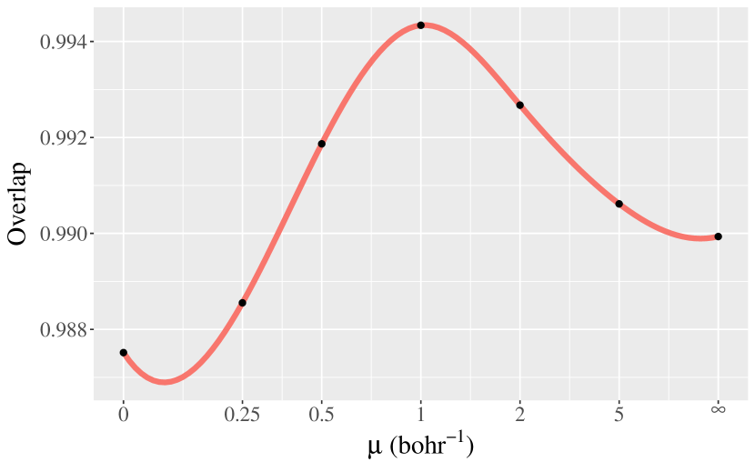
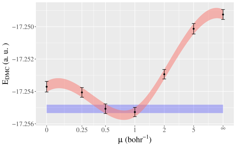
Figure 3: Left: Overlap between $\Psi^{\mu}$ and $\Psi^{J}$ as a function of $\mu$ for H2O. Right: FN-DMC energy of $\Psi^{\mu}$ (red curve) as a function of $\mu$, together with the FN-DMC energy of $\Psi^{J}$ (blue line) for H2O. The width of the lines represent the statistical error bars. For these two trial wave functions, the CI expansion consists of the 200 most important determinants of the FCI expansion obtained with the VDZ-BFD basis (see Sec. IV.2 for more details). The raw data can be found in the supplementary material.

As evidenced by Fig. 3, there is a clear maximum overlap between the two trial wave functions at $\mu=1$ bohr^-1, which coincides with the minimum of the FN-DMC energy of $\Psi^{\mu}$. Also, it is interesting to notice that the FN-DMC energy of $\Psi^{J}$ is compatible with that of $\Psi^{\mu}$ for $0.5<\mu<1$ bohr^-1, as shown by the overlap between the red and blue bands. This confirms that introducing short-range correlation with DFT has an impact on the CI coefficients similar to a Jastrow factor. This is another key result of the present study.

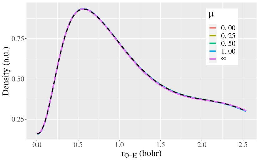
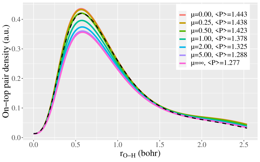
Figure 4: One-electron density $n(\mathbf{r})$ (left) and on-top pair density $n_{2}(\mathbf{r},\mathbf{r})$ (right) along the O-H axis of H2O as a function of $\mu$ for $\Psi^{\mu}$, and $\Psi^{J}$ (dashed curve). The integrated on-top pair density $\expectationvalue{P}$ is given in the legend. For all trial wave functions, the CI expansion consists of the 200 most important determinants of the FCI expansion obtained with the VDZ-BFD basis (see Sec. IV.2 for more details). The raw data can be found in the supplementary material.

In order to refine the comparison between $\Psi^{\mu}$ and $\Psi^{J}$, we report several quantities related to the one- and two-body densities of $\Psi^{J}$ and $\Psi^{\mu}$ with different values of $\mu$. First, we report in the legend of the right panel of Fig 4 the integrated on-top pair density

$$\expectationvalue{P}=\int d\mathbf{r}\,n_{2}(\mathbf{r},\mathbf{r}),$$ (14)

obtained for both $\Psi^{\mu}$ and $\Psi^{J}$, where $n_{2}(\mathbf{r}_{1},\mathbf{r}_{2})$ is the two-body density [normalized to $N(N-1)$]. Then, in order to have a pictorial representation of both the one-body density $n(\mathbf{r})$ and the on-top pair density $n_{2}(\mathbf{r},\mathbf{r})$, we report in Fig. 4 the plots of $n(\mathbf{r})$ and $n_{2}(\mathbf{r},\mathbf{r})$ along one of the O-H axis of the water molecule.

From these data, one can clearly notice several trends. First, the integrated on-top pair density $\expectationvalue{P}$ decreases when $\mu$ increases, which is expected as the two-electron interaction increases in $H^{\mu}[n]$. Second, Fig. 4 shows that the relative variations of the on-top pair density with respect to $\mu$ are much more important than that of the one-body density, the latter being essentially unchanged between $\mu=0$ and $\mu=\infty$ while the former can vary by about 10$\%$ in some regions. In the high-density region of the O-H bond, the value of the on-top pair density obtained from $\Psi^{J}$ is superimposed with $\Psi^{\mu=0.5}$, and at a large distance the on-top pair density of $\Psi^{J}$ is the closest to that of $\Psi^{\mu=\infty}$. The integrated on-top pair density obtained with $\Psi^{J}$ is $\expectationvalue{P}=1.404$, which nestles between the values obtained at $\mu=0.5$ and $\mu=1$ bohr^-1, consistently with the FN-DMC energies and the overlap curve depicted in Fig. 3.

These data suggest that the wave functions $\Psi^{0.5\leq\mu\leq 1}$ and $\Psi^{J}$ are close, and therefore that the operators that produced these wave functions (i.e., $H^{\mu}[n]$ and $e^{-J}He^{J}$) contain similar physics. Considering the form of $\hat{H}^{\mu}[n]$ [see Eq. (6)], one can notice that the differences with respect to the usual bare Hamiltonian come from the non-divergent two-body interaction $\hat{W}_{\text{ee}}^{\text{lr},\mu}$ and the effective one-body potential $\hat{\bar{V}}_{\text{Hxc}}^{\text{sr},\mu}[n]$ which is the functional derivative of the Hxc functional. The roles of these two terms are therefore very different: with respect to the exact ground-state wave function $\Psi$, the non-divergent two-body interaction increases the probability of finding electrons at short distances in $\Psi^{\mu}$, while the effective one-body potential $\hat{\bar{V}}_{\text{Hxc}}^{\text{sr},\mu}[n_{\Psi^{\mu}}]$, providing that it is exact, maintains the exact one-body density. This is clearly what has been observed in Fig. 4. Regarding now the transcorrelated Hamiltonian $e^{-J}He^{J}$, as pointed out by Ten-no,Ten-no (2000) the effective two-body interaction induced by the presence of a Jastrow factor can be non-divergent when a proper two-body Jastrow factor $J_{\text{ee}}$ is chosen, i.e., the Jastrow factor must fulfill the so-called electron-electron cusp conditions. Kato (1957); R. T. Pack and W. Byers-Brown (1966) There is therefore a clear parallel between $\hat{W}_{\text{ee}}^{\text{lr},\mu}$ in RS-DFT and $J_{\text{ee}}$ in FN-DMC. Moreover, the one-body Jastrow term $J_{\text{eN}}$ ensures that the one-body density remains unchanged when the CI coefficients are re-optmized in the presence of $J_{\text{ee}}$. There is then a second clear parallel between $\hat{\bar{V}}_{\text{Hxc}}^{\text{sr},\mu}[n]$ in RS-DFT and $J_{\text{eN}}$ in FN-DMC. Thus, one can understand the similarity between the eigenfunctions of $H^{\mu}$ and the optimization of the Slater-Jastrow wave function: they both deal with an effective non-divergent interaction but still produce a reasonable one-body density.

IV.3 Intermediate conclusions

As conclusions of the first part of this study, we can highlight the following observations:

• With respect to the nodes of a KS determinant or a FCI wave function, one can obtain a multi-determinant trial wave function $\Psi^{\mu}$ with a smaller fixed-node error by properly choosing an optimal value of $\mu$.

• The optimal $\mu$ value is system- and basis-set-dependent, and it grows with basis set size.

• Numerical experiments (overlap $\innerproduct*{\Psi^{\mu}}{\Psi^{J}}$, one-body density, on-top pair density, and FN-DMC energy) indicate that the RS-DFT scheme essentially plays the role of a simple Jastrow factor by mimicking short-range correlation effects. This latter statement can be qualitatively understood by noticing that both RS-DFT and the trans-correlated approach deal with an effective non-divergent electron-electron interaction, while keeping the density constant.

V Energy differences in FN-DMC: atomization energies

Atomization energies are challenging for post-HF methods because their calculation requires a subtle balance in the description of atoms and molecules. The mainstream one-electron basis sets employed in molecular electronic structure calculations are atom-centered, so they are, by construction, better adapted to atoms than molecules. Thus, atomization energies usually tend to be underestimated by variational methods. In the context of FN-DMC calculations, the nodal surface is imposed by the determinantal part of the trial wave function which is expanded in the very same atom-centered basis set. Thus, we expect the fixed-node error to be also intimately connected to the basis set incompleteness error. Increasing the size of the basis set improves the description of the density and of the electron correlation, but also reduces the imbalance in the description of atoms and molecules, leading to more accurate atomization energies. The size-consistency and the spin-invariance of the present scheme, two key properties to obtain accurate atomization energies, are discussed in Appendices A and B, respectively.

Table 2: Mean absolute errors (MAEs), mean signed errors (MSEs), and root mean square errors (RMSEs) with respect to the NIST reference values obtained with various methods and basis sets. All quantities are given in kcal/mol. The raw data can be found in the supplementary material.

		VDZ-BFD			VTZ-BFD			VQZ-BFD
Method	$\mu$	MAE	MSE	RMSE	MAE	MSE	RMSE	MAE	MSE	RMSE
PBE	0	$5.02$	$-3.70$	$6.04$	$4.57$	$1.00$	$5.32$	$5.31$	$0.79$	$6.27$
BLYP	0	$9.53$	$-9.21$	$7.91$	$5.58$	$-4.44$	$5.80$	$5.86$	$-4.47$	$6.43$
PBE0	0	$11.20$	$-10.98$	$8.68$	$6.40$	$-5.78$	$5.49$	$6.28$	$-5.65$	$5.08$
B3LYP	0	$11.27$	$-10.98$	$9.59$	$7.27$	$-5.77$	$6.63$	$6.75$	$-5.53$	$6.09$
CCSD(T)	$\infty$	$24.10$	$-23.96$	$13.03$	$9.11$	$-9.10$	$5.55$	$4.52$	$-4.38$	$3.60$
RS-DFT-CIPSI	0	$4.53$	$-1.66$	$5.91$	$6.31$	$0.91$	$7.93$	$6.35$	$3.88$	$7.20$
	1/4	$5.55$	$-4.66$	$5.52$	$4.58$	$1.06$	$5.72$	$5.48$	$1.52$	$6.93$
	1/2	$13.42$	$-13.27$	$7.36$	$6.77$	$-6.71$	$4.56$	$6.35$	$-5.89$	$5.18$
	1	$17.07$	$-16.92$	$9.83$	$9.06$	$-9.06$	$5.88$
	2	$19.20$	$-19.05$	$10.91$
	5	$22.93$	$-22.79$	$13.24$
	$\infty$	$23.63(4)$	$-23.49(4)$	$12.81(4)$	$8.43(39)$	$-8.43(39)$	$4.87(7)$	$4.51(78)$	$-4.18(78)$	$4.19(20)$
DMC@	0	$4.61(34)$	$-3.62(34)$	$5.30(09)$	$3.52(19)$	$-1.03(19)$	$4.39(04)$	$3.16(26)$	$-0.12(26)$	$4.12(03)$
RS-DFT-CIPSI	1/4	$4.04(37)$	$-3.13(37)$	$4.88(10)$	$3.39(77)$	$-0.59(77)$	$4.44(34)$	$2.90(25)$	$0.25(25)$	$3.745(5)$
	1/2	$3.74(35)$	$-3.53(35)$	$4.03(23)$	$2.46(18)$	$-1.72(18)$	$3.02(06)$	$2.06(35)$	$-0.44(35)$	$2.74(13)$
	1	$5.42(29)$	$-5.14(29)$	$4.55(03)$	$4.38(94)$	$-4.24(94)$	$5.11(31)$
	2	$5.98(83)$	$-5.91(83)$	$4.79(71)$
	5	$6.18(84)$	$-6.13(84)$	$4.87(55)$
	$\infty$	$7.38(1.08)$	$-7.38(1.08)$	$5.67(68)$
	Opt.	$5.85(1.75)$	$-5.63(1.75)$	$4.79(1.11)$

The atomization energies of the 55 molecules of the Gaussian-1 theoryPople et al. (1989); Curtiss et al. (1990) were chosen as a benchmark set to test the performance of the RS-DFT-CIPSI trial wave functions in the context of energy differences. Calculations were made in the double-, triple- and quadruple-$\zeta$ basis sets with different values of $\mu$, and using NOs from a preliminary CIPSI calculation as a starting point (see Fig. 1). For comparison, we have computed the energies of all the atoms and molecules at the KS-DFT level with various semi-local and hybrid density functionals [PBE, Perdew, Burke, and Ernzerhof (1996) BLYP, Becke (1988); Lee, Yang, and Parr (1988) PBE0, Perdew, Ernzerhof, and Burke (1996) and B3LYP Becke (1993)], and at the CCSD(T) level. Cizek ; Purvis III and Bartlett (1982); Scuseria, Janssen, and III (1988); Scuseria and III (1989) Table 2 gives the corresponding mean absolute errors (MAEs), mean signed errors (MSEs), and root mean square errors (RMSEs) with respect to the NIST reference values as explained in Sec. III. For FCI (RS-DFT-CIPSI, $\mu=\infty$) we have provided the extrapolated values (i.e., when $E_{\text{PT2}}\to 0$), and, although one cannot provide theoretically sound error bars, they correspond here to the difference between the extrapolated energies computed with a two-point and a three-point linear extrapolation. Loos et al. (2018, 2019a, 2020a, 2020b)

In this benchmark, the great majority of the systems are weakly correlated and are then well described by a single determinant. Therefore, the atomization energies calculated at the KS-DFT level are relatively accurate, even when the basis set is small. The introduction of exact exchange (B3LYP and PBE0) makes the results more sensitive to the basis set, and reduce the accuracy. Note that, due to the approximate nature of the xc functionals, the statistical quantities associated with KS-DFT atomization energies do not converge towards zero and remain altered even in the CBS limit. Thanks to the single-reference character of these systems, the CCSD(T) energy is an excellent estimate of the FCI energy, as shown by the very good agreement of the MAE, MSE and RMSE of CCSD(T) and FCI energies for each basis set. The imbalance in the description of molecules compared to atoms is exhibited by a very negative value of the MSE for CCSD(T)/VDZ-BFD ($-23.96$ kcal/mol) and FCI/VDZ-BFD ($-23.49\pm 0.04$ kcal/mol), which is reduced by a factor of two when going to the triple-$\zeta$ basis, and again by a factor of two when going to the quadruple-$\zeta$ basis.

This significant imbalance at the VDZ-BFD level affects the nodal surfaces, because although the FN-DMC energies obtained with near-FCI trial wave functions are much lower than the FN-DMC energies at $\mu=0$, the MAE obtained with FCI ($7.38\pm 1.08$ kcal/mol) is larger than the MAE at $\mu=0$ ($4.61\pm 0.34$ kcal/mol). Using the FCI trial wave function the MSE is equal to the negative MAE which confirms that the atomization energies are systematically underestimated. This corroborates that some of the basis set incompleteness error is transferred in the fixed-node error.

Within the double-$\zeta$ basis set, the calculations could be performed for the whole range of values of $\mu$, and the optimal value of $\mu$ for the trial wave function was estimated for each system by searching for the minimum of the spline interpolation curve of the FN-DMC energy as a function of $\mu$. This corresponds to the line labelled as “Opt.” in Table 2. The optimal $\mu$ value for each system is reported in the supplementary material. Using the optimal value of $\mu$ clearly improves the MAEs, MSEs, and RMSEs as compared to the FCI wave function. This result is in line with the common knowledge that re-optimizing the determinantal component of the trial wave function in the presence of electron correlation reduces the errors due to the basis set incompleteness. These calculations were done only for the smallest basis set because of the expensive computational cost of the QMC calculations when the trial wave function contains more than a few million determinants. Scemama et al. (2016) At the RS-DFT-CIPSI/VTZ-BFD level, one can see that the MAEs are larger for $\mu=1$ bohr^-1 ($9.06$ kcal/mol) than for FCI ($8.43\pm 0.39$ kcal/mol). The same comment applies to $\mu=0.5$ bohr^-1 with the quadruple-$\zeta$ basis.

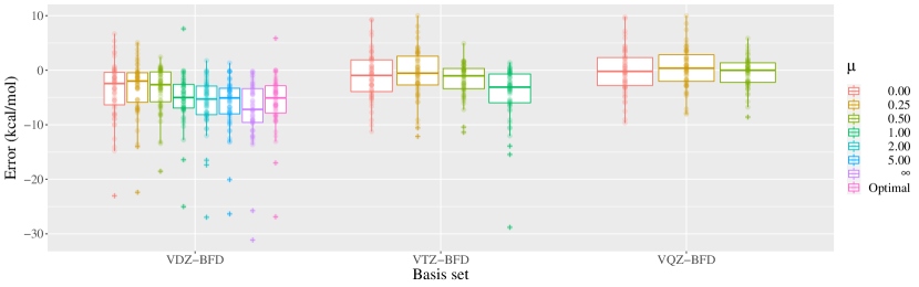
Figure 5: Errors in the FN-DMC atomization energies (in kcal/mol) for various trial wave functions $\Psi^{\mu}$ and basis sets. Each dot corresponds to an atomization energy. The boxes contain the data between first and third quartiles, and the line in the box represents the median. The outliers are shown with a cross. The raw data can be found in the supplementary material.

Searching for the optimal value of $\mu$ may be too costly and time consuming, so we have computed the MAEs, MSEs and RMSEs for fixed values of $\mu$. As illustrated in Fig. 5 and Table 2, the best choice for a fixed value of $\mu$ is $0.5$ bohr^-1 for all three basis sets. It is the value for which the MAE [$3.74(35)$, $2.46(18)$, and $2.06(35)$ kcal/mol] and RMSE [$4.03(23)$, $3.02(06)$, and $2.74(13)$ kcal/mol] are minimal. Note that these values are even lower than those obtained with the optimal value of $\mu$. Although the FN-DMC energies are higher, the numbers show that they are more consistent from one system to another, giving improved cancellations of errors. This is yet another key result of the present study, and it can be explained by the lack of size-consistency when one considers different $\mu$ values for the molecule and the isolated atoms. This observation was also mentioned in the context of optimally-tune range-separated hybrids. Stein, Kronik, and Baer (2009); Karolewski, Kronik, and Kummel (2013); Kronik et al. (2012)

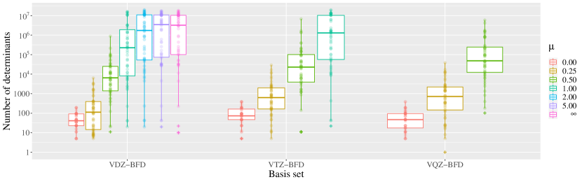
Figure 6: Number of determinants for various trial wave functions $\Psi^{\mu}$ and basis sets. Each dot corresponds to an atomization energy. The boxes contain the data between first and third quartiles, and the line in the box represents the median. The outliers are shown with a cross. The raw data can be found in the supplementary material.

The number of determinants in the trial wave functions are shown in Fig. 6. As expected, the number of determinants is smaller when $\mu$ is small and larger when $\mu$ is large. It is important to note that the median of the number of determinants when $\mu=0.5$ bohr^-1 is below $100\,000$ determinants with the VQZ-BFD basis, making these calculations feasible with such a large basis set. At the double-$\zeta$ level, compared to the FCI trial wave functions, the median of the number of determinants is reduced by more than two orders of magnitude. Moreover, going to $\mu=0.25$ bohr^-1 gives a median close to 100 determinants at the VDZ-BFD level, and close to $1\,000$ determinants at the quadruple-$\zeta$ level for only a slight increase of the MAE. Hence, RS-DFT-CIPSI trial wave functions with small values of $\mu$ could be very useful for large systems to go beyond the single-determinant approximation at a very low computational cost while ensuring size-consistency. For the largest systems, as shown in Fig. 6, there are many systems for which we could not reach the threshold $E_{\text{PT2}}<1$ m$E_{h}$ as the number of determinants exceeded 10 million before this threshold was reached. For these cases, there is then a small size-consistency error originating from the imbalanced truncation of the wave functions, which is not present in the extrapolated FCI energies (see Appendix A).

VI Conclusion

In the present work, we have shown that introducing short-range correlation via a range-separated Hamiltonian in a FCI expansion yields improved nodal surfaces, especially with small basis sets. The effect of short-range DFT on the determinant expansion is similar to the effect of re-optimizing the CI coefficients in the presence of a Jastrow factor, but without the burden of performing a stochastic optimization.

In addition to the intermediate conclusions drawn in Sec. IV.3, we have shown that varying the range-separation parameter $\mu$ and approaching RS-DFT-FCI with CIPSI provides a way to adapt the number of determinants in the trial wave function, leading to size-consistent FN-DMC energies. We propose two methods. The first one is for the computation of accurate total energies by a one-parameter optimization of the FN-DMC energy via the variation of the parameter $\mu$. The second method is for the computation of energy differences, where the target is not the lowest possible FN-DMC energies but the best possible cancellation of errors. Using a fixed value of $\mu$ increases the (size-)consistency of the trial wave functions, and we have found that $\mu=0.5$ bohr^-1 is the value where the cancellation of errors is the most effective. Moreover, such a small value of $\mu$ gives extremely compact wave functions, making this recipe a good candidate for the accurate description of the whole potential energy surfaces of large systems. If the number of determinants is still too large, the value of $\mu$ can be further reduced to $0.25$ bohr^-1 to get extremely compact wave functions at the price of less efficient cancellations of errors.

We hope to report, in the near future, a detailed investigation of strongly-correlated systems with the present RS-DFT-CIPSI scheme.

Data availability

The data that support the findings of this study are openly available in Zenodo at http://doi.org/10.5281/zenodo.3996568.

Appendix A Size consistency

An extremely important feature required to get accurate atomization energies is size-consistency (or strict separability), since the numbers of correlated electron pairs in the molecule and its isolated atoms are different.

KS-DFT energies are size-consistent, and because xc functionals are directly constructed in complete basis, their convergence with respect to the size of the basis set is relatively fast. Franck et al. (2015); Giner et al. (2018); Loos et al. (2019b); Giner et al. (2020) Hence, DFT methods are very well adapted to the calculation of atomization energies, especially with small basis sets. Giner et al. (2018); Loos et al. (2019b); Giner et al. (2020) However, in the CBS, KS-DFT atomization energies do not match the exact values due to the approximate nature of the xc functionals.

Likewise, FCI is also size-consistent, but the convergence of the FCI energies towards the CBS limit is much slower because of the description of short-range electron correlation using atom-centered functions. Kutzelnigg (1985); Kutzelnigg and Klopper (1991); Hattig et al. (2012) Eventually though, the exact atomization energies will be reached.

In the context of SCI calculations, when the variational energy is extrapolated to the FCI energy Holmes, Umrigar, and Sharma (2017) there is no size-consistency error. But when the truncated SCI wave function is used as a reference for post-HF methods such as SCI+PT2 or for QMC calculations, there is a residual size-consistency error originating from the truncation of the wave function.

QMC energies can be made size-consistent by extrapolating the FN-DMC energy to estimate the energy obtained with the FCI as a trial wave function.Scemama et al. (2018a, b) Alternatively, the size-consistency error can be reduced by choosing the number of selected determinants such that the sum of the PT2 corrections on the fragments is equal to the PT2 correction of the molecule, enforcing that the variational potential energy surface (PES) is parallel to the perturbatively corrected PES, which is a relatively accurate estimate of the FCI PES.Giner, Scemama, and Caffarel (2015)

Another source of size-consistency error in QMC calculations originates from the Jastrow factor. Usually, the Jastrow factor contains one-electron, two-electron and one-nucleus-two-electron terms. The problematic part is the two-electron term, whose simplest form can be expressed as in Eq. (12b). The parameter $a$ is determined by the electron-electron cusp condition, Kato (1957); R. T. Pack and W. Byers-Brown (1966) and $b$ is obtained by energy or variance minimization.Coldwell (1977); Umrigar and Filippi (2005) One can easily see that this parameterization of the two-body interaction is not size-consistent: the dissociation of a diatomic molecule AB with a parameter $b_{\ce{AB}}$ will lead to two different two-body Jastrow factors, each with its own optimal value $b_{\ce{A}}$ and $b_{\ce{B}}$. To remove the size-consistency error on a PES using this ansätz for $J_{\text{ee}}$, one needs to impose that the parameters of $J_{\text{ee}}$ are fixed, i.e., $b_{\ce{A}}=b_{\ce{B}}=b_{\ce{AB}}$.

When pseudopotentials are used in a QMC calculation, it is of common practice to localize the non-local part of the pseudopotential on the complete trial wave function $\Phi$. If the wave function is not size-consistent, so will be the locality approximation. Within the DLA,Zen et al. (2019) the Jastrow factor is removed from the wave function on which the pseudopotential is localized. The great advantage of this approximation is that the FN-DMC energy only depends on the parameters of the determinantal component. Using a non-size-consistent Jastrow factor, or a non-optimal Jastrow factor will not introduce an additional error in FN-DMC calculations, although it will reduce the statistical errors by reducing the variance of the local energy. Moreover, the integrals involved in the pseudopotential are computed analytically and the computational cost of the pseudopotential is dramatically reduced (for more details, see Ref. Scemama et al., 2015).

In this section, we make a numerical verification that the produced wave functions are size-consistent for a given range-separation parameter. We have computed the FN-DMC energy of the dissociated fluorine dimer, where the two atoms are separated by 50 Å. We expect that the energy of this system is equal to twice the energy of the fluorine atom. The data in Table 3 shows that this is indeed the case, so we can conclude that the proposed scheme provides size-consistent FN-DMC energies for all values of $\mu$ (within twice the statistical error bars).

Table 3: FN-DMC energy (in $E_{h}$) using the VDZ-BFD basis set and the srPBE functional of the fluorine atom and the dissociated F2 molecule for various $\mu$ values. The size-consistency error is also reported.

$\mu$	F	Dissociated F2	Size-consistency error
0.00	$-24.188\,7(3)$	$-48.377\,7(3)$	$-0.000\,3(4)$
0.25	$-24.188\,7(3)$	$-48.377\,2(4)$	$+0.000\,2(5)$
0.50	$-24.188\,8(1)$	$-48.376\,9(4)$	$+0.000\,7(4)$
1.00	$-24.189\,7(1)$	$-48.380\,2(4)$	$-0.000\,8(4)$
2.00	$-24.194\,1(3)$	$-48.388\,4(4)$	$-0.000\,2(5)$
5.00	$-24.194\,7(4)$	$-48.388\,5(7)$	$+0.000\,9(8)$
$\infty$	$-24.193\,5(2)$	$-48.386\,9(4)$	$+0.000\,1(5)$

Appendix B Spin invariance

Closed-shell molecules often dissociate into open-shell fragments. To get reliable atomization energies, it is important to have a theory which is of comparable quality for open- and closed-shell systems. A good check is to make sure that all the components of a spin multiplet are degenerate, as expected from exact solutions.

FCI wave functions have this property and yield degenerate energies with respect to the spin quantum number $m_{s}$. However, multiplying the determinantal part of the trial wave function by a Jastrow factor introduces spin contamination if the Jastrow parameters for the same-spin electron pairs are different from those for the opposite-spin pairs.Ten-no (2004) Again, when pseudopotentials are employed, this tiny error is transferred to the FN-DMC energy unless the DLA is enforced.

The context is rather different within KS-DFT. Indeed, mainstream density functionals have distinct functional forms to take into account correlation effects of same-spin and opposite-spin electron pairs. Therefore, KS determinants corresponding to different values of $m_{s}$ lead to different total energies. Consequently, in the context of RS-DFT, the determinant expansion is impacted by this spurious effect, as opposed to FCI.

In this Appendix, we investigate the impact of the spin contamination on the FN-DMC energy originating from the short-range density functional. We have computed the energies of the carbon atom in its triplet state with the VDZ-BFD basis set and the srPBE functional. The calculations are performed for $m_{s}=1$ (3 spin-up and 1 spin-down electrons) and for $m_{s}=0$ (2 spin-up and 2 spin-down electrons).

The results are reported in Table 4. Although the energy obtained with $m_{s}=0$ is higher than the one obtained with $m_{s}=1$, the bias is relatively small, i.e., more than one order of magnitude smaller than the energy gained by reducing the fixed-node error going from the single determinant to the FCI trial wave function. The largest spin-invariance error, close to $2$ m$E_{h}$, is obtained for $\mu=0$, but this bias decreases quickly below $1$ m$E_{h}$ when $\mu$ increases. As expected, with $\mu=\infty$ we observe a perfect spin-invariance of the energy (within the error bars), and the bias is not noticeable for $\mu=5$ bohr^-1.

Hence, at the FN-DMC level, the error due to the spin invariance with RS-DFT-CIPSI trial wave functions is below the chemical accuracy threshold, and is not expected to be problematic for the comparison of atomization energies.

Table 4: FN-DMC energy (in $E_{h}$) for various $\mu$ values of the triplet carbon atom with different values of $m_{s}$ computed with the VDZ-BFD basis set and the srPBE functional. The spin-invariance error is also reported.

$\mu$	$m_{s}=1$	$m_{s}=0$	Spin-invariance error
0.00	$-5.416\,8(1)$	$-5.414\,9(1)$	$+0.001\,9(2)$
0.25	$-5.417\,2(1)$	$-5.416\,5(1)$	$+0.000\,7(1)$
0.50	$-5.422\,3(1)$	$-5.421\,4(1)$	$+0.000\,9(2)$
1.00	$-5.429\,7(1)$	$-5.429\,2(1)$	$+0.000\,5(2)$
2.00	$-5.432\,1(1)$	$-5.431\,4(1)$	$+0.000\,7(2)$
5.00	$-5.431\,7(1)$	$-5.431\,4(1)$	$+0.000\,3(2)$
$\infty$	$-5.431\,6(1)$	$-5.431\,3(1)$	$+0.000\,3(2)$

References

- Schrödinger (1926) E. Schrödinger, Phys. Rev. 28, 1049 (1926).
- Pople (1999) J. A. Pople, Rev. Mod. Phys. 71, 1267 (1999).
- White (1992) S. R. White, Phys. Rev. Lett. 69, 2863 (1992).
- Booth, Thom, and Alavi (2009) G. H. Booth, A. J. W. Thom, and A. Alavi, J. Chem. Phys. 131, 054106 (2009).
- Thom (2010) A. J. W. Thom, Phys. Rev. Lett. 105, 263004 (2010).
- Xu, Uejima, and Ten-no (2018) E. Xu, M. Uejima, and S. L. Ten-no, Phys. Rev. Lett. 121, 113001 (2018).
- Motta and Zhang (2018) M. Motta and S. Zhang, WIREs Comput. Mol. Sci. 8, e1364 (2018).
- Deustua et al. (2018) J. E. Deustua, I. Magoulas, J. Shen, and P. Piecuch, J. Chem. Phys. 149, 151101 (2018).
- Eriksen and Gauss (2018) J. J. Eriksen and J. Gauss, J. Chem. Theory Comput. 14, 5180 (2018).
- Eriksen and Gauss (2019) J. J. Eriksen and J. Gauss, J. Chem. Theory Comput. 15, 4873 (2019).
- Ghanem, Lozovoi, and Alavi (2019) K. Ghanem, A. Y. Lozovoi, and A. Alavi, J. Chem. Phys. 151, 224108 (2019).
- Abrams and Sherrill (2005) M. L. Abrams and C. D. Sherrill, Chem. Phys. Lett. 412, 121 (2005).
- Bytautas and Ruedenberg (2009) L. Bytautas and K. Ruedenberg, Chem. Phys. 356, 64 (2009).
- Roth (2009) R. Roth, Phys. Rev. C 79, 064324 (2009).
- Giner, Scemama, and Caffarel (2013) E. Giner, A. Scemama, and M. Caffarel, Can. J. Chem. 91, 879 (2013).
- Knowles (2015) P. J. Knowles, Mol. Phys. 113, 1655 (2015).
- Holmes, Changlani, and Umrigar (2016) A. A. Holmes, H. J. Changlani, and C. J. Umrigar, J. Chem. Theory Comput. 12, 1561 (2016).
- Holmes, Umrigar, and Sharma (2017) A. A. Holmes, C. J. Umrigar, and S. Sharma, J. Chem. Phys. 147, 164111 (2017).
- Sharma et al. (2017) S. Sharma, A. A. Holmes, G. Jeanmairet, A. Alavi, and C. J. Umrigar, J. Chem. Theory Comput. 13, 1595 (2017).
- Evangelista (2014) F. A. Evangelista, J. Chem. Phys. 140, 124114 (2014).
- Liu and Hoffmann (2016) W. Liu and M. R. Hoffmann, J. Chem. Theory Comput. 12, 1169 (2016).
- Tubman et al. (2016) N. M. Tubman, J. Lee, T. Y. Takeshita, M. Head-Gordon, and K. B. Whaley, J. Chem. Phys. 145, 044112 (2016).
- Tubman et al. (2020) N. M. Tubman, C. D. Freeman, D. S. Levine, D. Hait, M. Head-Gordon, and K. B. Whaley, J. Chem. Theory Comput. 16, 2139 (2020).
- Per and Cleland (2017) M. C. Per and D. M. Cleland, J. Chem. Phys. 146, 164101 (2017).
- Zimmerman (2017) P. M. Zimmerman, J. Chem. Phys. 146, 104102 (2017).
- Ohtsuka and ya Hasegawa (2017) Y. Ohtsuka and J. ya Hasegawa, J. Chem. Phys. 147, 034102 (2017).
- Garniron et al. (2018) Y. Garniron, A. Scemama, E. Giner, M. Caffarel, and P. F. Loos, J. Chem. Phys. 149, 064103 (2018).
- Bender and Davidson (1969) C. F. Bender and E. R. Davidson, Phys. Rev. 183, 23 (1969).
- Huron, Malrieu, and Rancurel (1973) B. Huron, J. P. Malrieu, and P. Rancurel, J. Chem. Phys. 58, 5745 (1973).
- Buenker and Peyerimhoff (1974) R. J. Buenker and S. D. Peyerimhoff, Theor. Chim. Acta 35, 33 (1974).
- Booth and Alavi (2010) G. H. Booth and A. Alavi, J. Chem. Phys. 132, 174104 (2010).
- Cleland, Booth, and Alavi (2010) D. Cleland, G. H. Booth, and A. Alavi, J. Chem. Phys. 132, 041103 (2010).
- Daday et al. (2012) C. Daday, S. Smart, G. H. Booth, A. Alavi, and C. Filippi, J. Chem. Theory. Comput. 8, 4441 (2012).
- Motta et al. (2017) M. Motta, D. M. Ceperley, G. K.-L. Chan, J. A. Gomez, E. Gull, S. Guo, C. A. Jiménez-Hoyos, T. N. Lan, J. Li, F. Ma, A. J. Millis, N. V. Prokof’ev, U. Ray, G. E. Scuseria, S. Sorella, E. M. Stoudenmire, Q. Sun, I. S. Tupitsyn, S. R. White, D. Zgid, and S. Zhang (Simons Collaboration on the Many-Electron Problem), Phys. Rev. X 7, 031059 (2017).
- Chien et al. (2018) A. D. Chien, A. A. Holmes, M. Otten, C. J. Umrigar, S. Sharma, and P. M. Zimmerman, J. Phys. Chem. A 122, 2714 (2018).
- Loos et al. (2018) P. F. Loos, A. Scemama, A. Blondel, Y. Garniron, M. Caffarel, and D. Jacquemin, J. Chem. Theory Comput. 14, 4360 (2018).
- Loos et al. (2019a) P.-F. Loos, M. Boggio-Pasqua, A. Scemama, M. Caffarel, and D. Jacquemin, J. Chem. Theory Comput. 15, 1939 (2019a).
- Loos et al. (2020a) P. F. Loos, F. Lipparini, M. Boggio-Pasqua, A. Scemama, and D. Jacquemin, J. Chem. Theory Comput. 16, 1711 (2020a).
- Loos et al. (2020b) P. F. Loos, A. Scemama, M. Boggio-Pasqua, and D. Jacquemin, J. Chem. Theory Comput. 16, 3720 (2020b).
- Williams et al. (2020) K. T. Williams, Y. Yao, J. Li, L. Chen, H. Shi, M. Motta, C. Niu, U. Ray, S. Guo, R. J. Anderson, J. Li, L. N. Tran, C.-N. Yeh, B. Mussard, S. Sharma, F. Bruneval, M. van Schilfgaarde, G. H. Booth, G. K.-L. Chan, S. Zhang, E. Gull, D. Zgid, A. Millis, C. J. Umrigar, and L. K. Wagner (Simons Collaboration on the Many-Electron Problem), Phys. Rev. X 10, 011041 (2020).
- Eriksen et al. (2020) J. J. Eriksen, T. A. Anderson, J. E. Deustua, K. Ghanem, D. Hait, M. R. Hoffmann, S. Lee, D. S. Levine, I. Magoulas, J. Shen, N. M. Tubman, K. B. Whaley, E. Xu, Y. Yao, N. Zhang, A. Alavi, G. K.-L. Chan, M. Head-Gordon, W. Liu, P. Piecuch, S. Sharma, S. L. Ten-no, C. J. Umrigar, and J. Gauss, “The ground state electronic energy of benzene,” (2020), arXiv:2008.02678 [physics.chem-ph] .
- Evangelisti, Daudey, and Malrieu (1983) S. Evangelisti, J.-P. Daudey, and J.-P. Malrieu, Chem. Phys. 75, 91 (1983).
- Ten-no (2017) S. L. Ten-no, J. Chem. Phys. 147, 244107 (2017).
- Hohenberg and Kohn (1964) P. Hohenberg and W. Kohn, Phys. Rev. 136, B 864 (1964).
- Kohn (1999) W. Kohn, Rev. Mod. Phys. 71, 1253 (1999).
- Kohn and Sham (1965) W. Kohn and L. J. Sham, Phys. Rev. 140, A1133 (1965).
- Parr and Yang (1989) R. G. Parr and W. Yang, Density-Functional Theory of Atoms and Molecules (Oxford University Press, New York, 1989).
- Franck et al. (2015) O. Franck, B. Mussard, E. Luppi, and J. Toulouse, J. Chem. Phys. 142, 074107 (2015).
- Giner et al. (2018) E. Giner, B. Pradines, A. Ferté, R. Assaraf, A. Savin, and J. Toulouse, J. Chem. Phys. 149, 194301 (2018).
- Loos et al. (2019b) P. F. Loos, B. Pradines, A. Scemama, J. Toulouse, and E. Giner, J. Phys. Chem. Lett. 10, 2931 (2019b).
- Giner et al. (2020) E. Giner, A. Scemama, P. F. Loos, and J. Toulouse, J. Chem. Phys. 152, 174104 (2020).
- Becke (2014) A. D. Becke, J. Chem. Phys. 140, 18A301 (2014).
- Foulkes et al. (2001) W. M. C. Foulkes, L. Mitas, R. J. Needs, and G. Rajagopal, Rev. Mod. Phys. 73, 33 (2001).
- Austin, Zubarev, and Lester (2012) B. M. Austin, D. Y. Zubarev, and W. A. Lester, Chem. Rev. 112, 263 (2012).
- Needs et al. (2020) R. J. Needs, M. D. Towler, N. D. Drummond, P. L. Ríos, and J. R. Trail, J. Chem. Phys. 152, 154106 (2020).
- Reynolds et al. (1982) P. J. Reynolds, D. M. Ceperley, B. J. Alder, and W. A. Lester, J. Chem. Phys. 77, 5593 (1982).
- Ceperley (1991) D. M. Ceperley, J. Stat. Phys. 63, 1237 (1991).
- Nakano et al. (2020) K. Nakano, C. Attaccalite, M. Barborini, L. Capriotti, M. Casula, E. Coccia, M. Dagrada, C. Genovese, Y. Luo, G. Mazzola, A. Zen, and S. Sorella, arXiv (2020), 2002.07401 .
- Scemama et al. (2013) A. Scemama, M. Caffarel, E. Oseret, and W. Jalby, J. Comput. Chem. 34, 938 (2013).
- Kim et al. (2018) J. Kim, A. D. Baczewski, T. D. Beaudet, A. Benali, M. C. Bennett, M. A. Berrill, N. S. Blunt, E. J. L. Borda, M. Casula, D. M. Ceperley, S. Chiesa, B. K. Clark, R. C. Clay, K. T. Delaney, M. Dewing, K. P. Esler, H. Hao, O. Heinonen, P. R. C. Kent, J. T. Krogel, I. Kylänpää, Y. W. Li, M. G. Lopez, Y. Luo, F. D. Malone, R. M. Martin, A. Mathuriya, J. McMinis, C. A. Melton, L. Mitas, M. A. Morales, E. Neuscamman, W. D. Parker, S. D. P. Flores, N. A. Romero, B. M. Rubenstein, J. A. R. Shea, H. Shin, L. Shulenburger, A. F. Tillack, J. P. Townsend, N. M. Tubman, B. V. D. Goetz, J. E. Vincent, D. C. Yang, Y. Yang, S. Zhang, and L. Zhao, J. Phys.: Condens. Matter 30, 195901 (2018).
- Kent et al. (2020) P. R. C. Kent, A. Annaberdiyev, A. Benali, M. C. Bennett, E. J. L. Borda, P. Doak, H. Hao, K. D. Jordan, J. T. Krogel, I. Kylänpää, J. Lee, Y. Luo, F. D. Malone, C. A. Melton, L. Mitas, M. A. Morales, E. Neuscamman, F. A. Reboredo, B. Rubenstein, K. Saritas, S. Upadhyay, G. Wang, S. Zhang, and L. Zhao, J. Chem. Phys. 152, 174105 (2020).
- Umrigar and Filippi (2005) C. J. Umrigar and C. Filippi, Phys. Rev. Lett. 94, 150201 (2005).
- Scemama and Filippi (2006) A. Scemama and C. Filippi, Phys. Rev. B 73, 241101 (2006).
- Umrigar et al. (2007) C. J. Umrigar, J. Toulouse, C. Filippi, S. Sorella, and R. G. Hennig, Phys. Rev. Lett. 98, 110201 (2007).
- Toulouse and Umrigar (2007) J. Toulouse and C. J. Umrigar, J. Chem. Phys. 126, 084102 (2007).
- Toulouse and Umrigar (2008) J. Toulouse and C. J. Umrigar, J. Chem. Phys. 128, 174101 (2008).
- Petruzielo, Toulouse, and Umrigar (2012) F. R. Petruzielo, J. Toulouse, and C. J. Umrigar, J. Chem. Phys. 136, 124116 (2012).
- Dubecký et al. (2014) M. Dubecký, R. Derian, P. Jurečka, L. Mitas, P. Hobza, and M. Otyepka, Phys. Chem. Chem. Phys. 16, 20915 (2014).
- Grossman (2002) J. C. Grossman, J. Chem. Phys. 117, 1434 (2002).
- (70) J. Cizek, Adv. Chem. Phys. 14, 35.
- Purvis III and Bartlett (1982) G. D. Purvis III and R. J. Bartlett, J. Chem. Phys. 76, 1910 (1982).
- Per, Walker, and Russo (2012) M. C. Per, K. A. Walker, and S. P. Russo, J. Chem. Theory Comput. 8, 2255 (2012).
- Wang, Zhou, and Wang (2019) T. Wang, X. Zhou, and F. Wang, J. Phys. Chem. A 123, 3809 (2019).
- Filippi and Fahy (2000) C. Filippi and S. Fahy, J. Chem. Phys. 112, 3523 (2000).
- Haghighi Mood and Lüchow (2017) K. Haghighi Mood and A. Lüchow, J. Phys. Chem. A 121, 6165 (2017).
- Ludovicy, Mood, and Lüchow (2019) J. Ludovicy, K. H. Mood, and A. Lüchow, J. Chem. Theory Comput. 15, 5221 (2019).
- Bressanini (2012) D. Bressanini, Phys. Rev. B 86, 115120 (2012).
- Loos and Bressanini (2015) P.-F. Loos and D. Bressanini, J. Chem. Phys. 142, 214112 (2015).
- Giner, Scemama, and Caffarel (2015) E. Giner, A. Scemama, and M. Caffarel, J. Chem. Phys. 142, 044115 (2015).
- Caf (2016) “Recent Progress in Quantum Monte Carlo,” (2016), [Online; accessed 6. Jul. 2020].
- Caffarel et al. (2016) M. Caffarel, T. Applencourt, E. Giner, and A. Scemama, J. Chem. Phys. 144, 151103 (2016).
- Scemama et al. (2014) A. Scemama, T. Applencourt, E. Giner, and M. Caffarel, J. Chem. Phys. 141, 244110 (2014).
- Scemama et al. (2016) A. Scemama, T. Applencourt, E. Giner, and M. Caffarel, J. Comput. Chem. 37, 1866 (2016).
- Scemama et al. (2018a) A. Scemama, Y. Garniron, M. Caffarel, and P.-F. Loos, J. Chem. Theory Comput. 14, 1395 (2018a).
- Scemama et al. (2018b) A. Scemama, A. Benali, D. Jacquemin, M. Caffarel, and P.-F. Loos, J. Chem. Phys. 149, 034108 (2018b).
- Scemama et al. (2019) A. Scemama, M. Caffarel, A. Benali, D. Jacquemin, and P. F. Loos., Res. Chem. 1, 100002 (2019).
- Giner, Assaraf, and Toulouse (2016) E. Giner, R. Assaraf, and J. Toulouse, Mol. Phys. 114, 910 (2016).
- Dash et al. (2018) M. Dash, S. Moroni, A. Scemama, and C. Filippi, J. Chem. Theory Comput. 14, 4176 (2018).
- Dash et al. (2019) M. Dash, J. Feldt, S. Moroni, A. Scemama, and C. Filippi, J. Chem. Theory Comput. 15, 4896 (2019).
- Savin (1996a) A. Savin, in Recent Advances in Density Functional Theory, edited by D. P. Chong (World Scientific, 1996) pp. 129–148.
- Toulouse, Colonna, and Savin (2004) J. Toulouse, F. Colonna, and A. Savin, Phys. Rev. A 70, 062505 (2004).
- Garniron et al. (2019) Y. Garniron, T. Applencourt, K. Gasperich, A. Benali, A. Ferté, J. Paquier, B. Pradines, R. Assaraf, P. Reinhardt, J. Toulouse, P. Barbaresco, N. Renon, G. David, J.-P. Malrieu, M. Véril, M. Caffarel, P.-F. Loos, E. Giner, and A. Scemama, J. Chem. Theory Comput. 15, 3591 (2019).
- Levy (1979) M. Levy, Proc. Natl. Acad. Sci. U.S.A. 76, 6062 (1979).
- Lieb (1983) E. H. Lieb, Int. J. Quantum Chem. 24, 24 (1983).
- Savin (1996b) A. Savin, Theoretical and Computational Chemistry 4, 327 (1996b).
- Pulay (1980) P. Pulay, Chem. Phys. Lett. 73, 393 (1980).
- Pulay (1982) P. Pulay, J. Comput. Chem. 3, 556 (1982).
- Johnson (2002) R. Johnson, “Computational chemistry comparison and benchmark database, nist standard reference database 101,” (2002), http://cccbdb.nist.gov/.
- Burkatzki, Filippi, and Dolg (2007) M. Burkatzki, C. Filippi, and M. Dolg, J. Chem. Phys. 126, 234105 (2007).
- Burkatzki, Filippi, and Dolg (2008) M. Burkatzki, C. Filippi, and M. Dolg, J. Chem. Phys. 129, 164115 (2008).
- Scuseria, Janssen, and III (1988) G. E. Scuseria, C. L. Janssen, and H. F. S. III, J. Chem. Phys. 89, 7382 (1988).
- Scuseria and III (1989) G. E. Scuseria and H. F. S. III, J. Chem. Phys. 90, 3700 (1989).
- Frisch et al. (2016) M. J. Frisch, G. W. Trucks, H. B. Schlegel, G. E. Scuseria, M. A. Robb, J. R. Cheeseman, G. Scalmani, V. Barone, G. A. Petersson, H. Nakatsuji, X. Li, M. Caricato, A. V. Marenich, J. Bloino, B. G. Janesko, R. Gomperts, B. Mennucci, H. P. Hratchian, J. V. Ortiz, A. F. Izmaylov, J. L. Sonnenberg, D. Williams-Young, F. Ding, F. Lipparini, F. Egidi, J. Goings, B. Peng, A. Petrone, T. Henderson, D. Ranasinghe, V. G. Zakrzewski, J. Gao, N. Rega, G. Zheng, W. Liang, M. Hada, M. Ehara, K. Toyota, R. Fukuda, J. Hasegawa, M. Ishida, T. Nakajima, Y. Honda, O. Kitao, H. Nakai, T. Vreven, K. Throssell, J. A. Montgomery, Jr., J. E. Peralta, F. Ogliaro, M. J. Bearpark, J. J. Heyd, E. N. Brothers, K. N. Kudin, V. N. Staroverov, T. A. Keith, R. Kobayashi, J. Normand, K. Raghavachari, A. P. Rendell, J. C. Burant, S. S. Iyengar, J. Tomasi, M. Cossi, J. M. Millam, M. Klene, C. Adamo, R. Cammi, J. W. Ochterski, R. L. Martin, K. Morokuma, O. Farkas, J. B. Foresman, and D. J. Fox, “Gaussian˜16 Revision C.01,” (2016), gaussian Inc. Wallingford CT.
- Scemama et al. (2020) A. Scemama, E. Giner, A. Benali, T. Applencourt, and K. Gasperich, “Quantumpackage/qp2: Version 2.1.2,” (2020).
- Toulouse, Savin, and Flad (2004) J. Toulouse, A. Savin, and H.-J. Flad, Int. J. Quantum Chem. 100, 1047 (2004).
- Perdew, Burke, and Ernzerhof (1996) J. P. Perdew, K. Burke, and M. Ernzerhof, Phys. Rev. Lett. 77, 3865 (1996).
- Goll et al. (2006) E. Goll, H.-J. Werner, H. Stoll, T. Leininger, P. Gori-Giorgi, and A. Savin, Chem. Phys. 329, 276 (2006).
- Toulouse, Colonna, and Savin (2005) J. Toulouse, F. Colonna, and A. Savin, J. Chem. Phys. 122, 014110 (2005).
- Goll, Werner, and Stoll (2005) E. Goll, H.-J. Werner, and H. Stoll, Phys. Chem. Chem. Phys. 7, 3917 (2005).
- Applencourt, Gasperich, and Scemama (2018) T. Applencourt, K. Gasperich, and A. Scemama, arXiv (2018), 1812.06902 .
- Zen et al. (2019) A. Zen, J. G. Brandenburg, A. Michaelides, and D. Alfé, J. Chem. Phys. 151, 134105 (2019).
- Assaraf, Caffarel, and Khelif (2000) R. Assaraf, M. Caffarel, and A. Khelif, Phys. Rev. E 61, 4566 (2000).
- Francis and Charles (1969) B. S. Francis and H. N. Charles, Proc. R. Soc. Lond. A. 309, 209 (1969).
- Francis, Charles, and Wilfrid (1969a) B. S. Francis, H. N. Charles, and L. J. Wilfrid, Proc. R. Soc. Lond. A. 310, 43 (1969a).
- Francis, Charles, and Wilfrid (1969b) B. S. Francis, H. N. Charles, and L. J. Wilfrid, Proc. R. Soc. Lond. A. 310, 63 (1969b).
- Ten-no (2000) S. Ten-no, Chem. Phys. Lett. 330, 169 (2000).
- Luo (2010) H. Luo, J. Chem. Phys. 133, 154109 (2010).
- Yanai and Shiozaki (2012) T. Yanai and T. Shiozaki, J. Chem. Phys. 136, 084107 (2012).
- Cohen et al. (2019) A. J. Cohen, H. Luo, K. Guther, W. Dobrautz, D. P. Tew, and A. Alavi, J. Chem. Phys. 151, 061101 (2019).
- Nightingale and Melik-Alaverdian (2001) M. P. Nightingale and V. Melik-Alaverdian, Phys. Rev. Lett. 87, 043401 (2001).
- Kato (1957) T. Kato, Comm. Pure Appl. Math. 10, 151 (1957).
- R. T. Pack and W. Byers-Brown (1966) R. T. Pack and W. Byers-Brown, J. Chem. Phys. 45, 556 (1966).
- Pople et al. (1989) J. A. Pople, M. Head-Gordon, D. J. Fox, K. Raghavachari, and L. A. Curtiss, J. Chem. Phys. 90, 5622 (1989).
- Curtiss et al. (1990) L. A. Curtiss, C. Jones, G. W. Trucks, K. Raghavachari, and J. A. Pople, J. Chem. Phys. 93, 2537 (1990).
- Note (1) At , the number of determinants is not equal to one because we have used the natural orbitals of a preliminary CIPSI calculation, and not the srPBE orbitals. So the Kohn-Sham determinant is expressed as a linear combination of determinants built with NOs. It is possible to add an extra step to the algorithm to compute the NOs from the RS-DFT-CIPSI wave function, and re-do the RS-DFT-CIPSI calculation with these orbitals to get an even more compact expansion. In that case, we would have converged to the KS orbitals with , and the solution would have been the PBE single determinant.
- Becke (1988) A. D. Becke, Phys. Rev. A 38, 3098 (1988).
- Lee, Yang, and Parr (1988) C. Lee, W. Yang, and R. G. Parr, Phys. Rev. B 37, 785 (1988).
- Perdew, Ernzerhof, and Burke (1996) J. P. Perdew, M. Ernzerhof, and K. Burke, J. Chem. Phys. 22, 9982 (1996).
- Becke (1993) A. D. Becke, J. Chem. Phys. 98, 5648 (1993).
- Stein, Kronik, and Baer (2009) T. Stein, L. Kronik, and R. Baer, J. Am. Chem. Soc. 131, 2818 (2009).
- Karolewski, Kronik, and Kummel (2013) A. Karolewski, L. Kronik, and S. Kummel, J. Chem. Phys. 138, 204115 (2013).
- Kronik et al. (2012) L. Kronik, T. Stein, S. Refaely-Abramson, and R. Baer, J. Chem. Theory Comput. 8, 1515 (2012).
- Kutzelnigg (1985) W. Kutzelnigg, Theor. Chim. Acta 68, 445 (1985).
- Kutzelnigg and Klopper (1991) W. Kutzelnigg and W. Klopper, J. Chem. Phys. 94, 1985 (1991).
- Hattig et al. (2012) C. Hattig, W. Klopper, A. Kohn, and D. P. Tew, Chem. Rev. 112, 4 (2012).
- Coldwell (1977) R. L. Coldwell, Int. J. Quantum Chem. 12, 215 (1977).
- Scemama et al. (2015) A. Scemama, E. Giner, T. Applencourt, and M. Caffarel, “QMC using very large configuration interaction-type expansions,” Pacifichem, Advances in Quantum Monte Carlo (2015).
- Ten-no (2004) S. Ten-no, J. Chem. Phys. 121, 117 (2004).