Blindness of score-based methods to isolated components and mixing proportions

Abstract

Statistical tasks such as density estimation and approximate Bayesian inference often involve densities with unknown normalising constants. Score-based methods, including score matching, are popular techniques as they are free of normalising constants. Although these methods enjoy theoretical guarantees, a little-known fact is that they exhibit practical failure modes when the unnormalised distribution of interest has isolated components — they cannot discover isolated components or identify the correct mixing proportions between components. We demonstrate these findings using simple distributions and present heuristic attempts to address these issues. We hope to bring the attention of theoreticians and practitioners to these issues when developing new algorithms and applications.

1 Introduction and background

This paper presents a pervasive practical issue of score-based methods. The (HyvÀrinen) score function of a differentiable probability density $p(x)$ is defined by $s_{p}(x):=\nabla_{x}p(x)/p(x).$ Score function does not depend on the normaliser and, therefore, has a broad range of applications in machine learning and Bayesian statistics. Chief among these are the following: (a) training unnormalised density models with score matching (SM) [1], (b) measuring the quality of approximate samplers using Stein discrepancies (SDs) [3, 4, 5, 7, 14], and (c) approximate posterior sampling via Stein variational gradient descent (SVGD) [6]. We show that these theoretically well-motivated score-based algorithms can fail in practice when the unnormalised distribution has isolated components. In what follows, we exemplify the common failure modes with the following simple setup:

Example 1 (Gaussian mixtures).

Define the following density functions on $\mathbb{R}$:

$$p(x)=\pi_{1}p_{1}(x)+(1-\pi_{1})p_{2}(x),\,\,q(x)=p_{1}(x),\,\,p_{1}(x)=\mathcal{N}(x;-\mu,\sigma^{2}),\,p_{2}(x)=\mathcal{N}(x;\mu,\sigma^{2}).$$

where $\mu,\sigma>0$, and $\pi_{1}\in(0,1)$ are mixing proportions. In addition, we define $p^{\prime}(x):=\pi_{1}^{\prime}p_{1}(x)+(1-\pi_{1}^{\prime})p_{2}(x)$ as the same mixture as $p(x)$ but with a different mixing proportion $\pi_{1}^{\prime}\neq\pi_{1}$. Instances of these densities are shown in 1. When $\mu/\sigma^{2}$ is large, the components of $p$ are isolated.

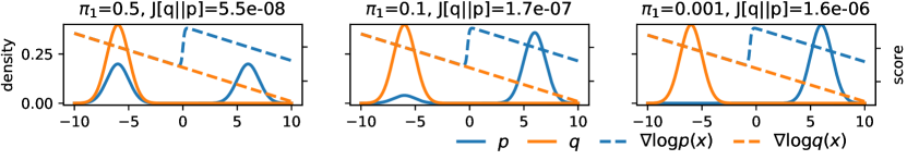
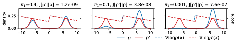
Figure 1: Distributions in 1 and their Fisher divergence (FD, $J$) for various choices of $\pi_{1}$ for the mixture $p$ (panel titles). Top, $J\!\left[{\color[rgb]{1,.5,0}q}\|{\color[rgb]{0,0,1}p}\right]$ is blind to the presence of an isolated component in the mixture $p$ regardless of $\pi_{1}$. Bottom, $J\!\left[{\color[rgb]{1,0,0}p^{\prime}}\|{\color[rgb]{0,0,1}p}\right]$ is blind to different mixing proportions.

The aforementioned failure modes stem from the following Lemma concerning the distributions in 1, the proof of which can be found in Appendix A.1.

Lemma 1 (Weak dependence of $s_{p}$ on $\pi_{1}$).

For the densities $p$ and $q$ defined in 1, $s_{p}(x)$ gets arbitrarily close to $s_{p_{1}}(x)=s_{q}(x)$ regardless of $\pi_{1}$ for $x\neq 0$ when $\mu/\sigma^{2}$ gets large.

This property is illustrated in 1 (top) — the score $s_{p}(x)$ does not change visibly with $\pi_{1}.$ In the following sections, we discuss the consequences of 1 for the three applications introduced above. To our knowledge, there has not been a synthesised exposition of the common failure modes, except for references [9, 13, 16, 15, 14, 17, 18] which on specific algorithms or other issues. We also propose heuristic remedies to initiate an effort to rectify these issues.

2 Fisher divergence and Stein discrepancy

Consider training an unnormalised density model $\tilde{p}(\boldsymbol{x})$ with score $s_{p}$ on data drawn from $q(x).$ [1] proposed SM to train $\tilde{p}$ by minimising the Fisher divergence (FD)

$$J[q||p]=\frac{1}{2}\int q(x)\left\|s_{q}(x)-s_{p}(x)\right\|_{2}^{2}\mathrm{d}x.$$

The FD is zero if and only if $p=q$. The densities $p$ and $q,$ however, can still be “very different” when their FD is close to but not exactly zero, as we show below (see also Appendix A.2).

Proposition 1 (FD is blind to isolated components).

For $q$ and $p$ in 1, the FD $J[q||p]\to 0$ regardless of the mixing proportion $\pi_{1}$ when $\mu/\sigma^{2}$ gets large.

Proof sketch.  The FD $J[q||p]$ is an expectation under $q$ which has almost all of its mass in $x<0$ as $\mu/\sigma^{2}$ gets large. 1 implies that $s_{p}(x)\to s_{p_{1}}(x)=s_{q}(x)$ for $x<0$. Thus, $J[q||p]\to 0.$

Another issue arises when two mixtures $p^{\prime}$ and $p$ comprise the same set of components weighted by different mixing proportions. In this case, their FD is almost zero despite the large difference in term of probability mass.

Proposition 2 (FD is blind to $\pi$).

For $p$(x) and $p^{\prime}(x)$ defined by distinct choices of the mixing proportion in 1, the FD $J(p^{\prime}\|p)\to 0$ as $\mu/\sigma^{2}$ gets large regardless of the mixing proportion.

Proof sketch.  By 1, the scores $s_{p}$ and $s_{p^{\prime}}$ converge to the same limit for $x\neq 0.$ They differ substantially only for $x$ close to 0 where $p^{\prime}$ puts vanishing mass, so $J(p^{\prime}\|p)\to 0$.

In density estimation where $p$ is the model, 1 implies that the model can have a mixture component far away from the data $q.$ According to 2, when isolated components in a data distribution $p^{\prime}$ are well-fit individually by the model $p$, one can obtain another model with small FD by varying the mixing proportions arbitrarily. See 1 (bottom row) for visualisations. We discuss in D.1 how previous successes of SM avoided these issues.

Next, we discuss the score-based Stein discrepancies (SDs) [3, 4, 5, 14] which can measure how well samples from $q$ agree with model $\tilde{p}$. A (Langevin) SD between $q$ and $p$ is defined as

$$\operatorname{SD_{\mathcal{F}}}\left[q\|p\right] =\sup_{f\in{\cal F}}\left|\mathbb{E}_{x\sim q}\!\left[s_{p}(x)^{\top}f(x)+\nabla_{x}^{\top}f(x)\right]\right|,$$ (1)

where $\nabla_{x}^{\top}$ is the divergence operator, and $\mathcal{F}$ is a class of differentiable vector-valued functions with appropriate boundary conditions (see the foregoing references for precise definitions). Since the SD is upper bounded by the FD (see Appendix A.3), we have the following:

Proposition 3 (Blindnesses of SD).

For $f\in\mathcal{F}$ such that $\int\|f(x)\|_{2}^{2}q(x)dx\leq 1$ and $q(x)f(x)\to 0$ as $\|x\|_{2}\to\infty$, $\mathrm{SD}_{\mathcal{F}}\!\left[q\|p\right]$ and $\mathrm{SD}_{\mathcal{F}}\!\left[p^{\prime}\|p\right]$ suffer from the issues of $J\left[q\|p\right]$ and $J\left[p^{\prime}\|p\right]$ in LABEL:prop:[s]spurious_mode and 2, respectively.

In the case of the kernel SD (KSD), where $\mathcal{F}$ is the unit ball of a reproducing kernel Hilbert space (RKHS) [4, 5], we show in 5 that the best $f\in\mathcal{F}$ witnessing the difference between $p$ and $q$ is almost zero around $x=0$. Therefore, diagnostics based on KSD can be misleading. We further discuss this issue in D.2 by relating to KSD bounds on integral probability metrics.

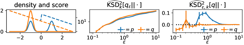
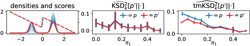
Figure 2: Top: densities (left) in 1 and their squared KSD (middle) and tmKSD (right) estimated with 500 samples. Bottom: the squared KSD (middle) and tmKSD (right) between ${\color[rgb]{1,0,0}p^{\prime}}$ and a few ${\color[rgb]{0,0,1}p}$ with various $\pi_{1}$ estimated with 2000 samples. Errorbar shows 1 s.e. estimated by Jackknife.

Heuristic remedy for KSD: matching a noisy $q$ and a tempered $p$

To better detect isolated components,consider adding noise to $q$ and changing the temperature of $p$:

$$q_{\epsilon}(x):=\int q(x^{\prime})\mathcal{N}(x|x^{\prime},\epsilon^{2})\mathrm{d}x^{\prime}\text{ where }\epsilon>0,\quad\tilde{p}^{\beta}(x)\propto\bigl{(}p(x)\bigr{)}^{\beta}\textrm{ where }\beta\in(0,1].$$

The KSD between $q_{\epsilon}$ and $\tilde{p}^{\beta}$ is given in closed-form [4, 5]:

$$\textrm{KSD}_{k}^{2}[q_{\epsilon}\|\tilde{p}^{\beta}] =\beta^{2}\mathbb{E}_{x,x^{\prime}\sim q_{\epsilon}}\!\left[s_{p}(x)^{\top}s_{p}(x^{\prime})k(x,x^{\prime})\right]+\beta\mathbb{E}_{x,x^{\prime}\sim q_{\epsilon}}\!\left[s_{p}(x)^{\top}\nabla_{x^{\prime}}k(x,x^{\prime})\right]$$

$$\quad\,+\beta\mathbb{E}_{x,x^{\prime}\sim q_{\epsilon}}\!\left[s_{p}(x^{\prime})^{\top}\nabla_{x}k(x,x^{\prime})\right]+\mathbb{E}_{x,x^{\prime}\sim q_{\epsilon}}\!\left[\mathrm{tr}[\nabla_{x}\nabla_{x^{\prime}}k(x,x^{\prime})]\right],$$ (2)

with $\mathrm{tr}$ the matrix trace. Adding noise to $q$ will likely increase this KSD, but we can adjust the temperature in $p$ to compensate for this effect, since both transformations “broaden” the original densities. By noting that (2) is convex and quadratic in $\beta$ for positive-definite $k$, we take its unique infimum over $\beta$ to counter the noise-induced mismatch, giving

$$\operatorname{\textrm{KSD}_{k,\epsilon}^{2}}[q\|p]:=\textrm{KSD}_{k}^{2}[q_{\epsilon}\|\tilde{p}^{\beta^{*}\!(\epsilon)}]\text{,$\quad$where\quad}\beta^{*}\!(\epsilon)=\operatorname*{\arg\min}_{\beta\in(0,1]}\textrm{KSD}_{k}^{2}[q_{\epsilon}\|\tilde{p}^{\beta}].$$ (3)

For the densities defined in 1, we visualise $\operatorname{\textrm{KSD}_{k,\epsilon}^{2}}\left[q\|p\right]$ as a function of $\epsilon$ and compare it with $\textrm{KSD}_{k}^{2}[q_{\epsilon}\|p]$ without temperature matching in 2 (top). For some values of $\epsilon$ $\operatorname{\textrm{KSD}_{k,\epsilon}^{2}}[q\|p]$ is significantly greater than the baseline $\operatorname{\textrm{KSD}_{k,\epsilon}^{2}}[q\|q]$ (right), but this is not the case for $\textrm{KSD}_{k}^{2}[q_{\epsilon}\|\cdot]$ (middle), suggesting the importance of matching the temperature with noise. Second, $\operatorname{\textrm{KSD}_{k,\epsilon}^{2}}$ reaches a maximum at some $\epsilon$. We define this maximum as the temperature-matched KSD

$$\textrm{tmKSD}_{k}^{2}\left[q\|p\right]:=\max_{\epsilon}\operatorname{\textrm{KSD}_{k,\epsilon}^{2}}\left[q\|p\right].$$

Note that this is not a valid discrepancy (see Appendix B), but it is more sensitive to isolated components than KSD. We show these SDs between a fixed $p^{\prime}$ and a few $p$ with various $\pi_{1}$ in 2 (bottom). Although $\textrm{tmKSD}_{k}^{2}\left[p^{\prime}\|p\right]$ still cannot reliably identify the correct mixing proportion 0.5, its smaller estimation errors and stronger dependence on $\pi_{1}$ compared to KSD are encouraging. We show very similar results for non-Gaussian distributions in Appendix B.

3 Stein variational gradient descent

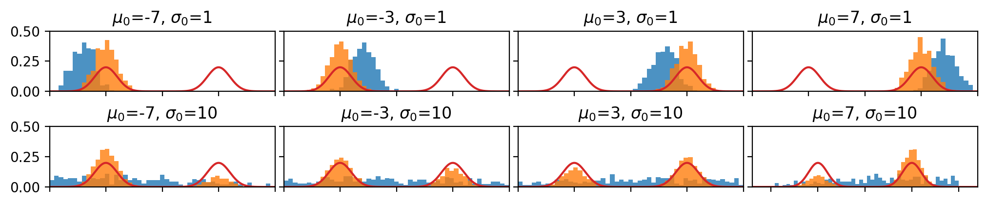
Figure 3: SVGD fails in approximating the target density $p$ (red) in 1. The initial $\nu_{0}$ is Gaussian $\mathcal{N}(\mu_{0},\sigma_{0}^{2})$ (blue) with small (top) or large (bottom) variances. Orange is the final $\nu_{t}$.

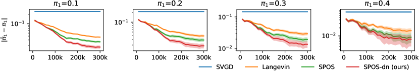
Figure 4: The difference between the fraction of particles $<0$ $(\hat{\pi}_{1})$ and the true mixing proportion ($\pi_{1}$) when running SVGD, LS, SPOS and the proposed SPOS-dn to approximate $p$ in 1. Lines are mean $\pm$ se estimated from 20 independent runs. See Appendix C for more results.

SVGD [6] approximates an unnormalised distribution $p$ by iteratively updating an empirical distribution $\nu_{t}$ formed by particles. The main idea is to find a direction $\phi$ such that the particle update $x\leftarrow x+\epsilon\phi(x)$ lowers the Kullback-Leibler divergence $\mathrm{KL}[\nu_{t}\|p]$. For $\phi$ defined by a function in the RKHS associated with a kernel $k(\cdot,\cdot)$, the optimal $\phi^{*}$ for a particle $x^{\prime}$ is given by

$$\phi^{*}(x^{\prime})=\mathbb{E}_{x\sim\nu_{t}}\!\left[s_{p}(x)k(x,x^{\prime})+\nabla_{x}k(x,x^{\prime})\right].$$ (4)

The particles can be initialised as samples drawn from a simple distribution $\nu_{0}$, such as a Gaussian with mean $m_{0}$ and variance $\sigma_{0}^{2}$.

Proposition 4 (Blindness of SVGD).

For the mixture $p$ in 1, if $\nu_{t}=q$ or $\nu_{t}=p^{\prime}$, one has that $\left\|\phi^{*}(x^{\prime})\right\|_{2}\to 0$ as $\mu/\sigma^{2}$ gets large.

Proof sketch. By the reproducing formula [2, Sec. 4.2], $\left\|\phi^{*}(x^{\prime})\right\|_{2}\leq\sqrt{k(x^{\prime},x^{\prime})}\operatorname{SD_{\mathcal{F}}}\left[\nu_{t}\|p\right]$, with ${\cal F}$ the unit ball of the RKHS. The upper bound goes to zero as $\mu/\sigma^{2}$ gets large by 3.

This means that the particles get stuck at $q$ or $p^{\prime}$, missing a component in $p$ completely or giving a wrong mixing proportions. We verify this empirically with results shown in 3. The final $\nu_{t}$ is highly sensitive to the initial $\nu_{0}$; contrary to intuitions, an overdispersed $\nu_{0}$ alone does not help.

Heuristic remedy: combine SVGD and Langevin sampling

Langevin sampling (LS) targets the same stationary distribution as SVGD while being more exploratory. A heuristic strategy is thus to update the particles according to a combination of LS and SVGD:

$$x^{\prime}\leftarrow x^{\prime}+\epsilon_{1}\mathbb{E}_{\nu_{t}}\!\left[s_{p}(x)k(x,x^{\prime})+\nabla_{x}k(x,x^{\prime})\right]+\epsilon_{2}s_{p}(x^{\prime})+\sqrt{2\epsilon_{2}}\omega,\quad\epsilon_{1},\epsilon_{2}\geq 0,\ \epsilon_{1}\epsilon_{2}\neq 0,$$ (5)

where $\omega$ is the standard normal. We let $\epsilon_{2}$ decrease gradually while keeping $\epsilon_{1}$ fixed. This is similar to SPOS [17] which reduces both $\epsilon_{1}$ and $\epsilon_{2}$, so we refer to our heuristic by SPOS-dn (decreasing the noisy LS step). We ran LS, SVGD, SPOS and SPOS-dn to sample $p$ in 1 and estimated the final mixing proportions. 4 shows that SPOS and SPOS-dn are better than LS and SVGD, and SPOS-dn converges the fastest. Nonetheless, finding the correct $\pi_{1}$ is still challenging for all algorithms tested. Details and additional results showing robustness to $\nu_{0}$ are in Appendix C.

Another approach proposed by [18] is to run SVGD while annealing $p$. However, unlike adding noise, annealing does not preserve the masses of isolated components (see Appendix D.3). Thus, this method still produces wrong mixing proportions [18, Fig. 4].

4 Discussion

We have demonstrated that three popular score-based methods fail to detect the isolated components or to identify the correct mixing proportions. The heuristic remedies presented here encourage more principled solutions. We stress that the practical failure modes presented here do not diminish, in any way, the theoretical advances of score-based methods; these methods have empowered practitioners to tackle a variety of statistical problems involving intractable distributions with unknown normalisers. Further, the issues discussed here may or may not impact certain downstream applications. For example, the model estimated by SM may still be suitable for local gradient-based methods, such as denoising. In contrast, unconditioned gradient-based sampling over the whole support may suffer from these issues. When using SVGD for Bayesian neural networks, ignoring the trivial posterior components arising from the symmetry of the weights does not affect the predictive distribution. We discuss other score-based methods that do not suffer from these issues in Appendix D.4.

Acknowledgement

We thank Maneesh Sahani and Arthur Gretton for useful discussions. This research is funded by the Gatsby Charitable Foundation.

Appendix A Proof

For notational simplicity we define $\pi_{2}:=1-\pi_{1}$.

A.1 Proof of 1

The score function is

$$\nabla_{x}\log p(x) =\frac{\pi_{1}\nabla_{x}p_{1}(x)+\pi_{2}\nabla_{x}p_{2}(x)}{\pi_{1}p_{1}(x)+\pi_{2}p_{2}(x)}$$

$$=-\frac{\pi_{1}\exp\left[-\frac{\left(x+\mu\right)^{2}}{2\sigma^{2}}\right]\frac{\left(x+\mu\right)}{\sigma^{2}}+\pi_{2}\exp\left[-\frac{\left(x-\mu\right)^{2}}{2\sigma^{2}}\right]\frac{\left(x-\mu\right)}{\sigma^{2}}}{\pi_{1}\exp\left[-\frac{\left(x+\mu\right)^{2}}{2\sigma^{2}}\right]+\pi_{2}\exp\left[-\frac{\left(x-\mu\right)^{2}}{2\sigma^{2}}\right]}$$

$$=-\frac{\pi_{1}\frac{\left(x+\mu\right)}{\sigma^{2}}+\pi_{2}\exp\left[\frac{\left(x+\mu\right)^{2}}{2\sigma^{2}}-\frac{\left(x-\mu\right)^{2}}{2\sigma^{2}}\right]\frac{\left(x-\mu\right)}{\sigma^{2}}}{\pi_{1}+\pi_{2}\exp\left[\frac{\left(x+\mu\right)^{2}}{2\sigma^{2}}-\frac{\left(x-\mu\right)^{2}}{2\sigma^{2}}\right]}$$

$$=-\frac{\pi_{1}\frac{\left(x+\mu\right)}{\sigma^{2}}+\pi_{2}\exp\left[2{\color[rgb]{0,0,1}\frac{\mu}{\sigma^{2}}}x\right]\frac{\left(x-\mu\right)}{\sigma^{2}}}{\pi_{1}+\pi_{2}\exp\left[2{\color[rgb]{0,0,1}{\color[rgb]{0,0,1}\frac{\mu}{\sigma^{2}}}}x\right]}$$

$$=-\left(\frac{x}{\sigma^{2}}+\frac{\pi_{1}-\pi_{2}\exp\left[2{\color[rgb]{0,0,1}\frac{\mu}{\sigma^{2}}}x\right]}{\pi_{1}+\pi_{2}\exp\left[2{\color[rgb]{0,0,1}{\color[rgb]{0,0,1}\frac{\mu}{\sigma^{2}}}}x\right]}\frac{\mu}{\sigma^{2}}\right).$$

In the limit of $\mu,\sigma^{2}$ such that ${\color[rgb]{0,0,1}\mu/\sigma^{2}}\to\infty$, we can see that

$$\left|\nabla_{x}\log p(x)-\left(-\frac{x+\mu}{\sigma^{2}}\right)\right|\to 0\ \text{for}\ x<0;$$

$$\left|\nabla_{x}\log p(x)-\left(-\frac{x-\mu}{\sigma^{2}}\right)\right|\to 0\ \text{for}\ x>0.$$

The two limits can be identified with $\nabla_{x}\log p_{1}(x)=-(x+\mu)/\sigma^{2}$ for $x<0$ and $\nabla_{x}\log p_{2}(x)=-(x-\mu)/\sigma^{2}$ for $x>0$ .

Remark 1.

A similar result holds for an arbitrary number of components without the Gaussian assumption. Consider a mixture of $K$ components with conditional likelihoods $p(x|z=k)$ for $k\in\{1,\dots,K\}$ that may differ across components. We say that the components are isolated if $p(z|x)$ is concentrated on a single component for all data points. In this case, we can write $s_{p}(x)$ as

$$s_{p}(x)=\frac{\nabla_{x}\int p(x|z)p(z)\mathrm{d}z}{p(x)}=\frac{\int\nabla_{x}\log p(x|z)p(x|z)p(z)\mathrm{d}z}{p(x)}=\sum_{k=1}^{K}p(z=k|x)\nabla_{x}\log p(x|z=k).$$

For a given $x$, if the posterior is concentrated on $z=k$, then it is clear that $s_{p}$ is approximately equal to $\nabla_{x}\log p(x|z=k)$, the score of the $k$th component.

A.2 Proof of 1

We split the integral in the definition of the Fisher divergence into the positive and negative parts. For the positive part, by the definition of $q,$ we have

$$\int_{0}^{\infty}q(x)\bigl{(}s_{q}(x)-s_{p}(x)\bigr{)}^{2}\mathrm{d}x =\int_{0}^{\infty}q(x)\bigl{(}s_{p}(x)-s_{p_{1}}(x)\bigr{)}^{2}\mathrm{d}x.$$

From the proof of 1, one can check that

$$\int q(x)\bigl{(}s_{p}(x)-s_{p_{1}}(x)\bigr{)}^{2}\mathrm{d}x =4\int q(x)\left(\frac{\pi_{2}\mu/\sigma^{2}}{\pi_{1}\exp\left[2x\mu/\sigma^{2}\right]+\pi_{2}}\right)^{2}\mathrm{d}x.$$

Since $\mu/\sigma^{2}>0$, for each point $x\in(0,\infty)$, the integrand converges to $0$ as $\mu/\sigma^{2}\to\infty$ and is bounded as

$$\left(\frac{\pi_{2}\mu/\sigma^{2}}{\pi_{1}\exp\left[2x\mu/\sigma^{2}\right]+\pi_{2}}\right)^{2}\leq\left(\frac{1}{2x}\frac{W\bigl{(}\pi_{2}/\pi_{1}\cdot e^{-1}\bigr{)}+1}{(\pi_{1}/\pi_{2})\exp\left\{W\bigl{(}\pi_{2}/\pi_{1}\cdot e^{-1}\bigr{)}+2x\right\}+1}\right)^{2},$$

with $W$ the Lambert W function. The upper bound is integrable with respect to the distribution $q.$ Thus, by the dominated convergence theorem, we have

$$\int_{0}^{\infty}q(x)\bigl{(}s_{p}(x)-s_{p_{1}}(x)\bigr{)}^{2}\mathrm{d}x\to 0\ \text{as}\ \frac{\mu}{\sigma^{2}}\to\infty.$$

The same conclusion can be similarly shown for the negative part, and therefore we have $J[q||p]\to 0$ regardless of the mixing proportion $\pi_{1}$ when $\mu/\sigma^{2}\to\infty$.

A.3 Proof of 3

Under the stated class $\mathcal{F}$, observe that

$$S_{\mathcal{F}}\left[q\|p\right] =\sup_{f\in{\cal F}}\left|\mathbb{E}_{q}\!\left[s_{p}(x)^{\top}f(x)+\nabla_{x}^{\top}f(x)\right]\right|$$

$$=\sup_{f\in{\cal F}}\left|\mathbb{E}_{q}\!\left[\{s_{p}(x)-s_{q}(x)\}^{\top}f(x)\right]\right|$$

$$\leq\sup_{\{f:\int f(x)^{2}q(x)dx\leq 1\}}\left|\mathbb{E}_{q}\!\left[\{s_{p}(x)-s_{q}(x)\}^{\top}f(x)\right]\right|$$

$$\leq\sqrt{\int\|s_{p}(x)-s_{q}(x)\|_{2}^{2}q(x)dx}\sup_{\{f:\int\lVert f(x)\rVert_{2}^{2}q(x)dx\leq 1\}}\sqrt{\int\|f(x)\|_{2}^{2}q(x)dx}$$

$$\leq\sqrt{2J[q\|p]}.$$

The second line is by integration by parts, the third line is from the integral assumption on ${\cal F}$, and the fourth line follows from the Cauchy-Schwartz inequality. As $J[q\|p]$ tends to zero as $\mu/\sigma^{2}\to\infty,$ so does the lower bound $S_{\mathcal{F}}\left[q\|p\right].$

To provide more intuition, we computed the optimal $f$ (witness function) for densities in 1 when $\mathcal{F}$ is given by the RKHS associated with a kernel $k$ (KSD)

$$\mathbb{E}_{q}\!\left[s_{p}(x)^{\top}k(x,\cdot)+\nabla_{x}^{\top}k(x,\cdot)\right]=\mathbb{E}_{q}\!\left[\{s_{p}(x)-s_{q}(x)\}^{\top}k(x,\cdot)\right].$$

We repeated this with both the Gaussian and IMQ kernels [7] with various bandwidths (0.5, 1.0, 2.0, 5.0 and 10.0). The results are shown in 5 in 5 for $q$ and $p$ and 6 for $p$ and $p^{\prime}$ with in 6. For all kernels and bandwidths, the witness functions are almost zero.

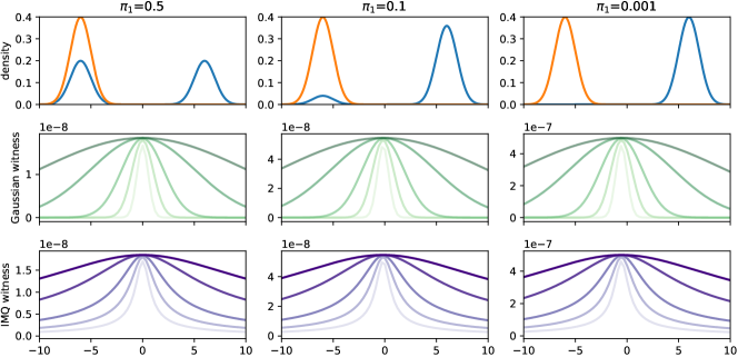
Figure 5: Top row, densities $p$ (blue) and $q$ (orange). Middle and bottom rows show witness functions for $\textrm{KSD}\left[q\|p\right]$ given by Gaussian and IMQ kernels, respectively. Darker colour indicates wider bandwidths of the kernels.

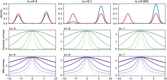
Figure 6: Same as 5 but for $\textrm{KSD}\left[p^{\prime}\|p\right]$ where $p^{\prime}$ (red) has a fixed mixing proportion $0.5$ and $p$ (blue) has mixing proportions indicated on at the top.

A.4 Proof of 4

For $x\in R^{d}$ and a reproducing kernel $k$ with associated RKHS $\mathcal{H}$, define

$$\xi_{i}(x,\cdot):=\mathbb{E}_{x\sim\nu_{t}}\!\left[s_{p,i}(x)k(x,\cdot)+\nabla_{x_{i}}k(x,\cdot)\right],\quad i\in\{1,\dots,d\}$$

By the reproducing property and Cauchy-Schwarz, we have

$$\left\|\phi^{*}(x^{\prime})\right\|_{2}^{2} =\sum_{i=1}^{d}\xi_{i}^{2}(x,x^{\prime})=\sum_{i=1}^{d}\left\langle k(x^{\prime},\cdot),\xi_{i}(x,\cdot)\right\rangle_{\mathcal{H}}^{2}$$

$$\leq\left\|k(x^{\prime},\cdot)\right\|_{\mathcal{H}}^{2}\sum_{i=1}^{d}\left\|\xi_{i}(x,\cdot)\right\|_{\mathcal{H}}^{2}=k(x^{\prime},x^{\prime})\mathrm{KSD}^{2}(\nu_{t}\|p),$$

where we followed the definition of $\mathcal{H}^{d}$ and KSD in [4].

Appendix B Temperature-matched Kernel Stein Discrepancy

B.1 Relative magnitude of tmKSD

In the example given in 2, we obtained a zero tmKSD between a Gaussian $q$ and itself. This is because adding zero-mean Gaussian noise to and changing the temperature of a Gaussian $q$ both yield another Gaussian, so it is always possible to find a value of $\beta$ such that $q_{\beta}=q_{\epsilon}$, giving a zero tmKSD as desired. If two Gaussian distributions $q$ and $p$ differ only in their variance, then KSD can easily detect the difference, while tmKSD cannot. Thus, tmKSD is better used to find specifically for isolated components after the usual KSD test.

More generally, when distributions are not restricted to Gaussians, then adding noise to and changing the temperature of the same distribution may result in nonzero KSDs. Thus, tmKSD is not a proper metric, and the absolute magnitude may not be indicative of goodness-of-fit. However, we see empirically that $\operatorname{\textrm{KSD}_{k,\epsilon}^{2}}[q\|q]$ is lower than $\operatorname{\textrm{KSD}_{k,\epsilon}^{2}}[q\|p]$ when $q\neq p$, which suggests that tmKSD may be used as a relative measure.

B.2 Experiments on other mixture distributions

To further validate the proposed tmKSD, we ran additional experiments on Laplace and Student-t distributions, which have heavier tails and more dispersed samples. The same experimental procedures as 2 are used here. The results for Laplace distributions are shown in 7, and those for Student-t (d.o.f 5.0) in 8. They are largely consistent with the results on the Gaussian distributions. Note that, for these distributions, the squared tmKSD between $q$ and $p$ is never smaller than that between $q$ and itself.

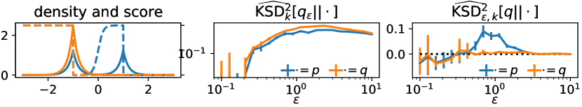
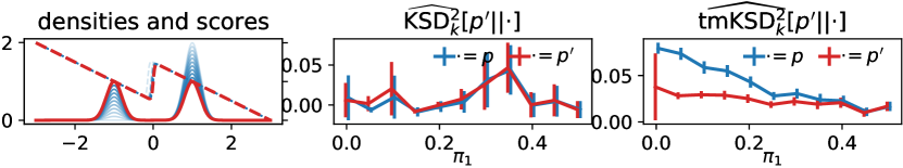
Figure 7: Same as 2 but for Laplace distribution and its mixtures.

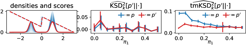
Figure 8: Same as 2 but for student-T distribution and its mixtures.

Appendix C Combining SVGD with LS

Empirically, we found that SVGD gave good solutions even with $\epsilon_{1}$ fixed at 1.0, so $\epsilon_{1}$ does not need to be decreased. Intuitively, LS contributes by mixing the initial particles to explore for isolated components, and SVGD “fine-tunes” the final particles thanks to the coupling between different particles.

We report the procedure and hyperparameters used for these experiments. For SVGD, we used $\epsilon=1.0$. For LS, we reduced the step size linearly from 1.0 to 0.0 at steps of 0.01. For the original SPOS, we reduced both $\epsilon_{1}$ and $\epsilon_{2}$ using the same linear schedule. For our SPOS-dn, we applied this linear schedule only to $\epsilon_{2}$ while keeping $\epsilon_{1}$ fixed at 1.0. All kernels used are squared-exponential with unit bandwidth. For each mixing proportion, we repeated each algorithm 20 times with different random seeds. To evaluate the effective mixing proportion of the final particles, we calculated the fraction of samples below 0.0 as $\hat{\pi}_{1}$ and report the error

$$\Delta\pi_{1}:=\left|\hat{\pi}_{1}-\pi_{1}\right|$$ (6)

where $\pi_{1}$ is the true mixing proportion in $p$.

The results in 4 were obtained when the initial distribution is $\nu_{0}=\mathcal{N}(0,1)$. We ran more simulations with $\nu_{0}$ sampled from $\mathcal{N}(-10.0,1)$ or $\mathcal{N}(10.0,1)$ and report all results in 9. In all settings, the proposed SPOS-dn gave the best estimated mixing proportions.

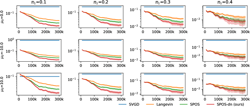
Figure 9: The trajectory of $\Delta\pi_{1}$ in (6) for SVGD, LS, SPOS and the proposed SPOS-dn to approximate the density $p$ in 1. Three rows are results from initial particles distributed as Gaussians with the indicated means and unit variance. Lines are mean $\pm$ se estimated from 20 independent runs.

Appendix D Further discussions

D.1 Previous successes with score matching

Previous successes on energy-based models required additional constraints preprocessing. To build a full probabilistic density model that supports all downstream statistical applications (e.g. density estimation, empirical Bayes, parameter interpretation, etc.), the issue of 1 can be partially alleviated by controlling the tail behaviour of $p$ [8, 16], although the notion of tails in a mixture distribution with isolated components may be harder to define. The issue of 2 can be partially addressed by fitting to each component after clustering the data [16]. [15] initiated a novel approach to training a sequence of score functions for sample generation, which gave very impressive results. However, this approach is not yet a generic learning algorithm for any given energy-based model for full downstream applications. More explicitly, the method of training a sequence of score functions is at odds with training a single energy-based model with a fixed architecture.

D.2 Isolated modes and Stein discrepancy bounds on integral probability metrics

Diffusion-based Stein discrepancies are known to upper-bound integral probability metrics (IPMs) such as the $L^{1}$-Wasserstein distance [3, 14] or the Dudley metric [7]. The key assumption in those results is that the diffusion has a fast Wasserstein decay rate as detailed in Section 2.2 of [14]; dissipativity conditions are sufficient for this requirement [14, Section 3]. A Gaussian mixture with a fixed shared variance satisfies the distant dissipativity condition. The $L^{1}$-Wasserstein rate of a diffusion targeting the distribution, however, can be slow, as shown in Proposition 3.4 of [10]; the rate has a factor exponential in the maximum distance between modes. Therefore, constants (known as Stein factors) appearing in the upper-bounds in the aforementioned papers can be large, and thus a small Stein discrepancy value might not imply the closeness in the IPM. This observation reflects the blindness of Stein discrepancies 3 – two Gaussian mixtures with largely different mixture weights should have different means and hence a large value of the $L^{1}$-Wasserstein distance.

D.3 Annealing does not preserve probability mass

[18] recently introduced this idea to SVGD and produced better samples. However, the mixing proportions are still incorrectly estimated. This is because annealing cannot preserve the mixing proportions between different temperatures.

Consider the mixture of two Gaussian with density shown in 10 (left). The probability masses round the two components change substantially as temperature varies, and they stay isolated. We manually pick a density threshold (middle, dashed black) below which we consider as low-density. When $\beta<0.5$, the density at $x=0.0$ is above the threshold for the support shown, and there are no isolated components; SVGD will correctly sample the distribution. When $\beta>0.5$, the components become isolated as the density at $x=0$ falls below the threshold in the green region (right), but the masses of the two components in the red and blue regions are still converging slowly to masses in the original mixture when $\beta=1$. Thus, when the particles are well-mixed at $\beta=0.5$, the proportions of particles allocated to $x<0$ and $x>0$ do not agree with the correct mixing proportions. The wrong mixing proportion are carried over into lower temperature up to $\beta=1$ (right, dotted lines). Note that this happens regardless of the annealing schedule.

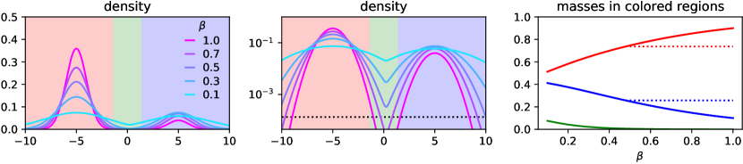
Figure 10: Left: densities of a Gaussian mixture at different temperatures $\beta$. Middle: log normalised densities of the mixtures. The dashed line delineates a threshold such that densities below this threshold is considered low, and very few samples exist. For illustrative purpose, this threshold is taken as the Gaussian density evaluated at 4 standard deviations from the mean. During annealing, the density at $x=0$ falls below the threshold as $\beta$ exceeds 0.5. Right, the mass in the middle green region becomes negligible when $\beta>0.5$ even when the masses in the red and blue regions are changing substantially. This means that during annealing there are hardly any samples that would appear in or transition through the green region. The relative sample proportion as $\beta$ increase beyond 0.5 is almost the same as when $\beta=0.5$, following the dotted lines, while the true proportions continue to change, following the solid lines.

D.4 Entropy gradient estimation does not suffer from the blindness

The score function appears in estimating the gradient of entropy of implicit distributions, e.g. [11, 12]. Consider an implicit distribution $p_{\phi}(x)$ defined by the mapping $f_{\phi}:z\mapsto x$, $z\sim\zeta$ where $\zeta$ is some simple distribution and $f_{\phi}$ is a flexible function parametrised by $\phi$. The gradient of the entropy satisfies

$$\nabla_{\phi}\mathbb{H}[p_{\phi}(x)]=\mathbb{E}_{\zeta\left(z\right)}\!\left[\nabla_{x}\log p_{\phi}(x)\nabla_{\phi}f_{\phi}(z)\right].$$

There are two reasons why this application does not suffer from the blindness discussed here. First, samples from $p(x)$ can be easily drawn from the implicit distribution, unlike when $p$ is an energy-based model. Second, the expectation above is an expectation of a $p_{\phi}(x)$-dependent function under $p_{\phi}(x)$ itself (through $\zeta$), which cannot be blind to itself. This is unlike SM or SD where the expectation involves two different density functions $p(x)$ and $q(x)$.

References

- [1] Aapo Hyvärinen “Estimation of non-normalized statistical models by score matching” In Journal of Machine Learning Research 6.Apr, 2005, pp. 695–709
- [2] Ingo Steinwart and Andreas Christmann “Support vector machines”, Information Science and Statistics Springer, New York, 2008
- [3] Jackson Gorham and Lester Mackey “Measuring sample quality with Stein’s method” In Advances in Neural Information Processing Systems, 2015
- [4] Kacper Chwialkowski, Heiko Strathmann and Arthur Gretton “A Kernel Test of Goodness of Fit” In ICML, 2016
- [5] Qiang Liu, Jason D. Lee and Michael Jordan “A Kernelized Stein Discrepancy for Goodness-of-fit Tests” In ICML, 2016
- [6] Qiang Liu and Dilin Wang “Stein variational gradient descent: A general purpose bayesian inference algorithm” In Advances in neural information processing systems, 2016
- [7] Jackson Gorham and Lester Mackey “Measuring sample quality with kernels” In International Conference on Machine Learning, 2017 PMLR
- [8] Michael Arbel and Arthur Gretton “Kernel Conditional Exponential Family” In AISTATS, 2018
- [9] Michael Arbel, D.. Sutherland, Mikolaj Binkowski and Arthur Gretton “On gradient regularizers for MMD GANs” In Advances in Neural Information Processing Systems, 2018
- [10] Murat A. Erdogdu, Lester Mackey and Ohad Shamir “Global Non-convex Optimization with Discretized Diffusions” In Advances in Neural Information Processing Systems, 2018
- [11] Yingzhen Li and Richard E. Turner “Gradient Estimators for Implicit Models” In International Conference on Learning Representations, 2018
- [12] Jiaxin Shi, Shengyang Sun and Jun Zhu “A Spectral Approach to Gradient Estimation for Implicit Distributions” In International Conference on Machine Learning, 2018
- [13] Jingwei Zhuo, Chang Liu, Jiaxin Shi, Jun Zhu, Ning Chen and Bo Zhang “Message passing Stein variational gradient descent” In International Conference on Machine Learning, 2018 PMLR
- [14] Jackson Gorham, Andrew B Duncan, Sebastian J Vollmer and Lester Mackey “Measuring sample quality with diffusions” In The Annals of Applied Probability 29.5 Institute of Mathematical Statistics, 2019
- [15] Yang Song and Stefano Ermon “Generative modeling by estimating gradients of the data distribution” In Advances in Neural Information Processing Systems, 2019
- [16] Li K. Wenliang, D.. Sutherland, Heiko Strathmann and Arthur Gretton “Learning deep kernels for exponential family densities” In ICML, 2019
- [17] Jianyi Zhang, Ruiyi Zhang, Lawrence Carin and Changyou Chen “Stochastic particle-optimization sampling and the non-asymptotic convergence theory” In International Conference on Artificial Intelligence and Statistics, 2020 PMLR
- [18] Francesco D’Angelo and Vincent Fortuin “Annealed stein variational gradient descent” In Third Symposium on Advances in Approximate Bayesian Inference, 2021