Measuring the stellar population parameters of the early-type galaxy NGC 3923 - The challenging measurement of the initial mass function

Abstract

Recent studies of early-type galaxies have suggested that the initial mass function (IMF) slope is bottom-heavy, i.e. they contain a larger fraction of low-mass stars than the Milky Way. However, measurements of the IMF remain challenging in unresolved galaxies because features in their observed spectra are sensitive to a number of factors including the stellar age, metallicity, and elemental abundances, in addition to the IMF. In this paper, we use new high signal-to-noise IMACS (Magellan) spectra to study the elliptical shell galaxy NGC 3923 at optical (3700–6600 Å), and near-infrared (7900–8500 Å) wavelengths, as a function of radius. We have undertaken a number of independent approaches to better understand the uncertainties in our results. 1) We compare two different stellar population model libraries; 2) we undertake spectral index fitting as well as full spectral fitting; 3) we have performed simulations for which we a priori know the input IMF, and which closely match our data; 4) we also investigate the effects of including a two-component, rather than a single stellar population. We show that our results are sensitive to the assumptions we make and to the methods we use. In addition, we evaluate the accuracy and precision of our results based on simulated mock data. We find some indication (although assumption-dependent) for a bottom-heavy IMF in the mass-range 0.5–1.0 $M_{\sun}$, while the IMF in the mass-range 0.08–0.5 $M_{\sun}$ appears to be Milky-Way like and constant. Including near-infrared data to our analysis gives consistent results, and improves the precision.

1 Introduction

Is the IMF universal (similar to what is observed in the Milky Way), or does it vary as a function of environment? The answer to this simple question remains elusive and important. For example, this question has serious implications for photometric and spectroscopic studies of the high-redshift universe. If the IMF varies widely in different environments, interpreting the star formation history with redshift becomes vastly more challenging.

The star formation histories of galaxies can be complex. Most stellar populations do not have a unique age or metallicity, but rather have unknown a priori distributions of those parameters. Analogously, there are no individual spectral features that are unique markers of age and metallicity; rather various features reflect those parameters in differing amounts. Spectral modeling is required to disentangle the information in the observed spectra of galaxies. Accurate spectral modeling requires that the libraries of stellar spectra reflect those of the galaxies being studied. Elliptical galaxies have higher metallicities than stars within the Milky Way. Furthermore, the abundances of the alpha elements are greater than observed in the solar neighborhood. Ensuring that the libraries are complete remains a serious challenge.

In the midst of these already challenging degeneracies is the unknown IMF. A further challenge comes from the fact that much of the integrated light in an elliptical galaxy results from the contribution of its brighter giant stars, while the fainter main sequence stars contribute little. There are only a few (generally weak) features that provide clues about the ratio of giant to dwarf stars, and whether the IMF is varying. It is not surprising therefore, that there remain conflicting conclusions in the literature concerning whether the IMF varies.

In this paper, the first in a series, we have studied the stellar population in the elliptical galaxy, NGC 3923. In later papers, we will explore a larger sample of elliptical galaxies, our own Milky Way bulge, and the integrated light of star clusters. Given the inherent difficulties in modeling stellar populations, in this study we have applied several independent approaches to the analysis of the same galaxy: we have used different models, undertaken simulations, and incorporated different types of spectral analysis. We wish to ask how model-dependent, or how spectral-analysis dependent any resulting conclusions might be.

We have explored both individual spectral-index fitting (following the procedure outlined in La Barbera et al., 2013; Martín-Navarro et al., 2015a; La Barbera et al., 2016), as well as full-spectral fitting (following Vaughan et al., 2018a, b, and using their code). For a more comprehensive overview of relevant literature in this field we refer the reader to Section 2. In this work, we incorporate two different models: the MILES/E-MILES models of Vazdekis et al. (2010, 2015, 2016), and the Conroy models (Conroy & van Dokkum, 2012a; Conroy et al., 2018). We have undertaken simulations (Lonoce et al. in preparation), in which we know a priori the underlying stellar population, and which we fit in the same way as the data for NGC 3923. Our goal has been to ascertain whether, despite modeling uncertainties and underlying degeneracies, we can find robust evidence for an IMF that differs from that observed in the Milky Way. We test if optical spectra alone can be used to constrain the IMF, or if near-infrared data are required. We compare the different methods, wavelength regions, and SPS models to understand the effects of different assumptions on the measurements.

This paper is organized as follows: We discuss previous studies of the IMF in Section 2. We present our data and measure spectral indices in Section 3. We use those indices for a stellar population analysis in Section 4. In Section 5 we apply full-spectral fitting as second approach. We compare our different approaches with those in the literature in Section 6, and summarize our results in Section 7.

2 Previous Work and Context

Our understanding of galaxies and galaxy evolution depends heavily on assumptions regarding the stellar initial mass function (IMF), which parameterizes the shape of the initial stellar mass distribution for a population of stars. A galaxy consisting of a stellar population with a top-heavy IMF, i.e. a larger fraction of high-mass stars, evolves faster, has more stellar feedback, a higher [$\alpha$/Fe] abundance, larger amounts of dust and metals, and more stellar remnants. On the other hand, a bottom-heavy IMF, leads to a slower chemical enrichment in the galaxy, and a larger fraction of M dwarf stars. The IMF determines several observables of a galaxy, such as the color, total luminosity, mass-to-light ratio, half-light radius, and star-formation rates (Bekki, 2013; Barber et al., 2018).

IMF studies have had a long history, but to date there is still debate about whether the IMF is universal. The first measurements of the IMF were made using field stars of the Milky Way. Salpeter (1955) parameterized the IMF in the form of a single power-law, with $dN/d\text{log}m\propto m^{-\Gamma}$, where $m$ is the initial mass of a star as it reaches the main sequence, $N$ is the number of stars in a logarithmic mass bin. The IMF slope $\Gamma$ was measured to be 1.35. Later studies found that a single power-law overestimates the number of stars with lower masses than the Sun in the Milky Way, and the IMF flattens and turns over at stellar masses 0.5–1 $M_{\sun}$ (Kroupa, 2001; Chabrier, 2003). Recent studies of resolved stellar populations in the Milky Way find similar IMF slopes for field stars, several star clusters and associations (e.g. Bastian et al., 2010; Krumholz, 2014, and references therein), with only few possible exceptions, which are still under debate. In addition, the high-mass IMF slopes in the LMC and SMC are compatible with the Milky Way’s IMF (Massey, 2003; Sabbi et al., 2008; Da Rio et al., 2009).

Theoretical considerations, however, suggest a dependence of the IMF on various physical processes and conditions during star formation, such as fragmentation, turbulence, accretion, magnetic fields, stellar interactions, feedback, or metallicity (e.g. Bonnell et al., 2007; Li et al., 2010; Hopkins, 2013; Bekki, 2013; Chabrier et al., 2014). Until now, no star formation theory has been able to implement all effects and predict their combined influence on the IMF.

It is important to measure the IMF in different galaxies, to get a better understanding of the processes that shape it, and how the IMF influences the evolution of a galaxy. The IMF may be non-universal and change for different environments, and stellar populations formed at different times.

In the past decade, several studies have measured the IMF beyond the Local Group, using integrated light observations and stellar population synthesis (SPS) models. Two basic approaches have been used. In the first approach one computes the mass-to-light ratio (M/L) of SPS models with different IMFs and compares them to the measured M/L of a galaxy. The stellar M/L can be derived using stellar kinematics and dynamical modeling (e.g. Cappellari et al., 2012, 2013; Lyubenova et al., 2016), gravitational lensing (e.g. Ferreras et al., 2008, 2010; Sonnenfeld et al., 2012; Leier et al., 2016) or a combination of both (e.g. Treu et al., 2010; Auger et al., 2010; Thomas et al., 2011b; Spiniello et al., 2011; Newman et al., 2017). However, the derived stellar M/L is dependent on the assumed dark matter distribution of a galaxy. Most studies assume a constant stellar M/L, but this is not necessarily true, as the stellar populations of galaxies change with radius. Constraining both the dark matter distribution and a possible stellar M/L gradient is a degenerate problem. Further, this method only allows one to exclude certain IMF shapes, but is unable to distinguish if a high M/L is caused by a bottom-heavy IMF, with many low-mass stars, or a top-heavy IMF, with many high-mass stars that evolved to dark remnants.

The second approach to measuring the IMF is to compare the integrated light spectra with SPS model spectra. Several spectral features in a galaxy spectrum are sensitive to the surface gravity of a star. The integrated light of a galaxy with an old stellar population is a mixture of the light from massive and bright giant stars, and less massive and faint, but more abundant dwarf stars. A galaxy spectrum changes depending on the ratio of dwarf stars to giant stars. This technique was used in several studies (e.g. Cenarro et al., 2003; van Dokkum & Conroy, 2010, 2012; Conroy & van Dokkum, 2012b; La Barbera et al., 2013; Spiniello et al., 2014; Martín-Navarro et al., 2015b, c; Martín-Navarro et al., 2019, and many others), and these authors found early-type galaxies with a higher fraction of low-mass stars than the Milky Way. Some galaxies have indications of an IMF gradient, with a higher fraction of low-mass stars in the galaxy center (Martín-Navarro et al., 2015a; van Dokkum et al., 2017; Sarzi et al., 2018), while other studies have found galaxies with a constant IMF (Alton et al., 2017, 2018; Vaughan et al., 2018a). However, in addition to the IMF, the stellar age, metallicity, elemental abundances, and star formation history influence spectral lines. These parameters can have a stronger influence on certain spectral features than the IMF has, and there are correlations and degenerate solutions. If the surface-gravity sensitive effects can be disentangled from abundance and star-formation history effects, then it may be possible to constrain the low-mass end of the IMF in early-type galaxies. For these reasons, it remains a challenging task to measure the IMF slope.

Previous studies (e.g. La Barbera et al., 2016, 2017; Sarzi et al., 2018; Vaughan et al., 2018b) have generally used spectra in the optical ($\sim$4000-6500 Å) to near-infrared wavelength range (>8000 Å). While longer wavelength spectra are more sensitive to low-mass stars, they are also more expensive in terms of observing time.

Table 1: Summary of observations

Date	Grating	Slit	Exposure	Position angle
		width	time	wrt major axis
2015-05-19	600$\ell$/9$\fdg$78	2$\farcs$5	1200 s $\times$ 3	0°
2015-05-20	600$\ell$/9$\fdg$82	2$\farcs$5	1200 s $\times$ 4	0°
2015-05-19	600$\ell$/16$\fdg$6	2$\farcs$5	1200 s $\times$ 3	0°
2018-05-11	600$\ell$/10$\fdg$46	2$\farcs$5	1200 s $\times$ 2	48°
2018-05-11	600$\ell$/10$\fdg$46	2$\farcs$5	770 s $\times$ 1	48°

3 Data

In this section we give an overview of our observations, our data reduction techniques, and describe the quality of our data. Our target is NGC 3923, an E4-5 galaxy with more than twenty symmetric shells (Prieur, 1988), located in the constellation of Hydra. NGC 3923 is at a distance of 30-33 Mpc, it belongs to the NGC 3923 group at redshift $z$=0.0046 (Garcia, 1993; Mulchaey et al., 2003).

3.1 Observations

We observed NGC 3923 on three nights: May 19, 2015, May 20, 2015, and May 11, 2018 with IMACS (Dressler et al., 2006), on the Magellan Baade 6.5-meter telescope. The observations were obtained with the $f$/4 camera, which provides a slit length of 15 arcmin, in slow read-out mode. In 2015, the slit was placed along the galaxy’s major axis. For the observation on May 11, 2018, the position angle was at 48° with respect to the major axis, along the Galactic North-South. The slit length is larger than NGC 3923, which has an effective radius of $R_{h}$=86$\farcs$4 (Ho et al., 2011), and thus allows simultaneous sky observations. In May 2015, we additionally observed blank fields on the sky. The IMACS detector consists of eight chips with 2048 wavelength pixels$\times$4096 spatial pixels each. Combined they give a 8192 pixel $\times$ 8192 pixel mosaic with one spatial gap and three wavelength gaps. We placed the slit such that the galaxy falls entirely on the upper part of the slit, and only on four of the eight detector chips. We used a slit width of 2$\farcs$5, and different gratings to provide greater wavelength coverage. For the two nights in 2015, we had the 600$\ell$/9$\fdg$78 and 600$\ell$/9$\fdg$82 grating to cover the spectrum at $\lambda$=3380–6725 Å, and the 600$\ell$/16$\fdg$6 grating to cover 7800–8600 Å; for the night in May 2018 we used the 600$\ell$/10$\fdg$46 grating and covered $\lambda$=3900–7120 Å. Exposure times were 1200 s, however, one exposure taken in 2018-05-11 was shorter (770 s), because the telescope was approaching zenith. We summarize the observations in Table 2.

3.2 Data reduction

3.2.1 Instrumental calibrations

Each detector chip was reduced separately, including bias subtraction, cosmic ray removal, distortion correction, wavelength calibration, sky subtraction, flat fielding, and flux calibration using idl and iraf scripts.

We estimated the bias using the overscan region of each chip, and subtracted it. With the idl routine l.a.cosmic (van Dokkum, 2001) we identified cosmic rays and created bad pixel masks. We rectified the distortion along chip rows by tracing several emission lines on the He/Ne/Ar arc lamp exposures. For each night, we took pinhole exposures, and we used those to trace the distortion along chip columns. We used the iraf tasks identify, reidentify, and fitcoords for simultaneous wavelength calibration to air wavelengths. The wavelength gaps between individual chips are 10–20 Å wide.

We traced the position of the galaxy along the slit as a function of wavelength by fitting a Cauchy function to the galaxy light profile. We fit various arc lines close to the galaxy trace to estimate the spectral resolution $R=\lambda/\Delta\lambda$. $R$ is increasing with wavelength, from about $R$=675 at $\lambda$=3900 Å to about $R$=1150 at $\lambda$=6700 Å, and $R$=1500 at $\lambda$=8000 Å for a slit width of 2$\farcs$5.

3.2.2 Spectral extraction and telluric correction

We extracted the one-dimensional spectra from each exposure in several radial bins. The central spectrum was extracted in a 1$\farcs$5 wide region, further at distances of 0$\farcs$75–3″ from the center, 3″–$\frac{1}{8}$ $R_{h}$, $\frac{1}{8}$ $R_{h}$–¼ $R_{h}$, ¼ $R_{h}$–½ $R_{h}$, ½ $R_{h}$–$\frac{3}{4}$ $R_{h}$, ½ $R_{h}$–1 $R_{h}$, and $\frac{3}{4}$ $R_{h}$–1 $R_{h}$. We adopted 1 $R_{h}$=86$\farcs$4 and summed the respective regions in the upper and lower part of the slit together. For the spectra observed on 2018-05-11, we corrected for the different P.A. as follows: We assumed an ellipticity of $\epsilon$=0.271, and modified the extraction regions such that they contain the same isophote regions as the observations along the major axis.

Further, we extracted the sky from a region > 3 $R_{h}$ from the galaxy and subtracted it from the spectra, see Appendix A.1 for details. We applied flat fielding and flux calibration, derived from standard star observations (Feige 67 and Hip 59167) taken on the same nights.

The spectra have telluric absorption lines from H₂O and O₂ molecules in the Earth’s atmosphere. We used the ESO tool molecfit (Smette et al., 2015; Kausch et al., 2015) to correct the atmospheric absorption. molecfit creates a synthetic atmosphere spectrum and derives a correction function, taking the spectral resolution into account. Molecular absorption lines vary with time. The advantage of molecfit is that it uses the science observations directly and not observations of a telluric standard star, taken at a different time than the target. We derived the atmospheric absorption correction for each exposure using the central spectrum, and applied the same correction to all spectra.

We fit the atmospheric absorption in the wavelength regions 6253–6300 Å, 6820–6976 Å, and 8170–8300 Å and made sure that these regions are free of prominent emission or absorption lines. Example spectra with the applied molecfit correction are shown in Fig.1. The spectra before telluric correction are in red, and spectra after telluric correction are in black. We show spectra observed on different nights, and extracted for different regions, to cover a wide range of S/N. Telluric correction in the region 6270 Å is satisfactory, but there are sky residuals at 6295–6305 Å (two upper spectra), which led us to perform a second order sky subtraction (see Appendix A.2). There are some residuals from telluric correction at 6870 Å (see also Fig. 15) for spectra with lower S/N. We excluded this spectral region from our analysis.

Figure 1: Spectra of NGC 3923 before (red) and after (black) telluric absorption correction. The upper panel shows three exposures observed on three different nights in the wavelength region 6250–6320 Å. The three different spectra were extracted at different regions of the galaxy; some of them have sky residuals around 6300 Å. For one of the three exposures, observed 2018-05-11, the chip gap starts at 6290 Å. The lower panel shows two out of three exposures observed 2018-05-11, in the longer wavelength region 6800–7000 Å, also at different distances from the galaxy’s center.

After applying these corrections, we summed the different exposures taken at the same nights to one spectrum per night and IMACS chip. Finally, we performed a second order sky subtraction (see Appendix A.2) and used the velocity measurements to shift each spectrum to rest wavelength.

3.2.3 Data quality

We combined the spectra of the two 2015 nights to obtain the final spectra as a function of distance from the center of NGC 3923. As the 2018 observations were taken at a different P.A. and grating angle, we did not sum the 2018 spectra together with the 2015 spectra. As result, we have a set of spectra in the optical wavelength region 3500–6640 Å, observed along the major axis and as a function of galactocentric radius (shown in Fig. 15), and another set of spectra in the optical wavelength region 3900–7050 Å, at a P.A. 48° offset from the galaxy major axis (Fig. 16). In addition, we have spectra in the near-infrared wavelength region 7800–8600 Å along the major axis (Fig. 21). Due to the longer total exposure time (2h 20 min), the optical spectra along the major axis have a higher S/N than the spectra along P.A.=48° (53 min), and the near-infrared spectra along the major axis (60 min).

We show the signal-to-noise ratio (S/N) of the optical spectra as a function of wavelength for each spectrum in Fig. 2; the different colors denote the extraction regions. The S/N is lowest in the blue end of the spectrum, $\lambda$< 4000Å. Except for the outermost spectrum, we have a S/N$\gtrsim$200 Å^-1 for the P.A.=0° spectra at $\lambda$>4500 Å. Our near-infrared spectra (7800–8600 Å) have S/N $\approx$ 400 in the center, decreasing to $\approx$ 100 in the outer three bins. For the P.A.=48° spectra, the S/N does not exceed 200 Å^-1 for the outer four spectra. Recent studies used spectra with S/N$\gtrsim$100 Å^-1 (e.g. Martín-Navarro et al., 2015a; Sarzi et al., 2018) for spectral index fitting. Some of our spectra also exceed the S/N of the spectra used by van Dokkum & Conroy (2012) and Conroy & van Dokkum (2012b), which go up to 400 Å^-1 at 5000 Å. Thus, our data have S/N that is comparable or even higher than the S/N of data used in other studies.

Figure 2: Signal-to-noise ratio of the spectra as a function of wavelength for different extraction radii, for spectra with P.A.=0° on the upper panel, and P.A. = 48° on the lower panel. Grey shaded regions mark chip gaps.

3.3 Measurements

In the following section we describe our procedure for measuring stellar kinematics, gas emission, and spectral indices on our optical spectra. For the spectral indices we account for the effects of resolution, and non-Gaussian line-of-sight velocity distribution (LOSVD).

3.3.1 Stellar kinematics and emission line correction

We fit the stellar LOSVD of the final combined spectra with the program pPXF (Cappellari & Emsellem, 2004; Cappellari, 2017) and SSP templates. The SSP models are convolved with a LOSVD, to obtain the four best-fit kinematic moments (V, $\sigma$, $h_{3}$, $h_{4}$). Together with the kinematics, we fit an optimal template, which is a linear combination of the input SSP templates.

To obtain the correct kinematic solution, it is important that the template library contains spectra that match the stellar populations of the data. For this reason, we used a wide range of stellar parameters for the template models. In particular, we used the E-MILES SSP models (Vazdekis et al., 2016) with a bimodal IMF parameterization, with 14 different IMF slopes (see Sect. 4.1.2 for details), 15 ages (1–17.8 Gyr), and 6 metallicities (-1.7 to +0.2 dex). See Appendix B for an overview of SSP models.

We measured the stellar kinematics in the spectral ranges 3760–6640 Å (P.A.=0°) and 3920–6700 Å (P.A.=48°), with additive polynomials (10th and 12th order, respectively) to correct the model continuum shape. We masked bad pixels for the fit. To account for the possibility of gas emission, we used the code GandALF (Gas AND Absorption Line Fitting) by Sarzi et al. (2006) to fit stellar populations and gas emission simultaneously. We fixed the stellar kinematics and fit the spectra with multiplicative polynomials (10th and 12th order, respectively). The fit emission lines were subtracted from the spectra if their amplitudes were three times higher than the noise in the respective spectral region. This was fulfilled for the Balmer lines in the outer four spectra along the major axis.

Given that the spectra have been shifted to rest wavelength (Appendix A.2), the resulting velocities are close to zero. The velocity dispersion in the center reaches 275 km s^-1, but decreases down to 170 km s^-1 at 54″ and beyond. The Gauss-Hermite moments h₃ and h₄ are within -0.01<h₃<0.02 and 0.07<h₄<0.14. This means that the LOSVD is nearly symmetric, as the skewness $h_{3}$ is close to zero. The positive kurtosis $h_{4}$ indicates that the LOSVD is more heavy-tailed than a Gaussian, possibly due to a radial velocity anisotropy. We list our kinematic results in Table 3.3.1. We derived the uncertainties from the dispersion of 500 Monte Carlo runs, in which we added random noise to the spectra before measuring the LOSVD.

Table 2: LOSVD results for P.A.=0° data

radius	$\sigma$	$h_{3}$	$h_{4}$
(arcsec)	(km$\cdot$ s-1)
0.00	276.0 $\pm$ 2.7	-0.01 $\pm$ 0.01	0.08 $\pm$ 0.01
1.85	270.1 $\pm$ 2.6	-0.01 $\pm$ 0.01	0.08 $\pm$ 0.01
6.90	244.3 $\pm$ 2.6	-0.01 $\pm$ 0.01	0.10 $\pm$ 0.01
16.20	210.3 $\pm$ 3.1	-0.00 $\pm$ 0.01	0.11 $\pm$ 0.01
32.40	196.3 $\pm$ 3.9	0.00 $\pm$ 0.01	0.11 $\pm$ 0.01
54.00	174.0 $\pm$ 6.9	0.00 $\pm$ 0.01	0.13 $\pm$ 0.03
64.80	169.7 $\pm$ 7.3	0.01 $\pm$ 0.01	0.13 $\pm$ 0.03
75.60	170.3 $\pm$ 12.5	0.02 $\pm$ 0.02	0.14 $\pm$ 0.06

3.3.2 Spectral index measurements

We interpolated over bad pixels and measured spectral indices (as listed in Table 3) on both the final combined spectra and, if needed, on the emission-line subtracted spectra. If we omit the subtraction, the value of several Balmer line indices changes (see red diamonds and blue circle symbols in Fig. 3), leading to a different age estimate by several Gyr. By subtracting the gas emission, we ensure that the spectral index measures stellar population rather than gas. Our procedure to derive spectral index uncertainties is described in Appendix A.3.

Table 3: Spectral index definitions

Index	blue continuum [Å]	feature    [Å]	red continuum    [Å]	type	reference
H$\gamma\sigma_{275}$	4331.500 – 4341.00	4331.500 – 4351.875	4359.250 – 4368.750	A	1
H$\beta$	4827.875 – 4847.875	4847.875 – 4876.625	4876.625 – 4891.625	A	2
Fe4383	4359.125 – 4370.375	4369.125 – 4420.375	4442.875 – 4455.375	A	2
Fe5270	5233.150 – 5248.150	5245.650 – 5285.650	5285.650 – 5318.150	A	2
Fe5335	5304.625 – 5315.875	5312.125 – 5352.125	5353.375 – 5363.375	A	2
Mgb	5142.625 – 5161.375	5160.125 – 5192.625	5191.375 – 5206.375	A	2
Ca4592	4502.500 – 4512.000	4578.000 – 4603.000	4611.000 – 4628.000	A	3
Fe5709	5672.875 – 5696.625	5696.625 – 5720.375	5722.875 – 5736.625	A	2
Fe5782	5765.375 – 5775.375	5776.625 – 5796.625	5797.875 – 5811.625	A	2
bTiO	4742.750 – 4756.500	4758.500 – 4800.000	4827.875 – 4847.875	M	4
aTiO	5420.000 – 5442.000	5445.000 – 5600.000	5630.000 – 5655.000	M	4
TiO2	6066.625 – 6141.625	6189.625 – 6272.125	6372.625 – 6415.125	M	2

Note. — Kinematic uncertainties are statistical only

3.3.3 Resolution and LOSVD correction

To constrain the stellar populations of NGC 3923, we compared our measured spectral indices with those indices from SSP models. For a meaningful comparison, data and model indices must be measured at the same resolution. However, each observed spectrum has a different resolution because of the varying velocity dispersion, and a different non-zero h₃ and h₄ (see Sect. 3.3.1). Both, velocity broadening and non-Gaussian LOSVD, affect the spectral index measurements (Kuntschner, 2004). Before comparing our data with the model indices, we therefore corrected for the different resolutions and non-Gaussian LOSVDs as follows.

First, we chose a common resolution for our data and model reference indices. Spectral line indices are often measured in the “Line Index System" (LIS, Vazdekis et al., 2010) with a resolution of FWHM=14 Å. Due to velocity broadening, the FWHM of the three central NGC 3923 spectra is higher than the reference value of FWHM=14 Å, whereas the outer spectra have a higher resolution and lower FWHM. For the data with higher resolution, we simply convolved the spectra to FWHM=14 Å before measuring spectral indices.

In order to derive a correction for the lower resolution data and non-Gaussian LOSVD, we measured the line indices not only on the data, but also on our best-fit model spectra obtained with pPXF. We measured the indices on two sets of best-fit model spectra: On the best-fit model spectrum at the LIS reference spectral resolution (FWHM=14 Å, with h₃ = h₄ = 0), and on the best-fit spectrum that was convolved with the same LOSVD as measured on the data with pPXF. The difference of these two measurements is nonzero, which confirms that the broader FWHM caused by the high velocity dispersion, and the non-Gaussian LOSVD of our data should not be ignored. We used the ratio of these two model index measurements as factor to transfer our atomic index measurements (measured in units of Å) to the LIS (i.e. h₃ = h₄ = 0 and FWHM=14 Å). This factor changes the index measurements of our data by up to 20%. For molecular indices (measured in magnitudes), the correction is not a factor but the difference of the two best-fit model measurements. Also for indices that can have negative values (e.g. H$\delta_{A}$, H$\delta_{F}$, H$\gamma_{A}$, H$\gamma_{F}$), the correction is additive (Kuntschner, 2004). After this correction, we can compare the index measurements of our data to indices measured on SSP models.

Figure 3: Absorption line index gradients measured for NGC 3923. Open red diamonds denote index measurements without emission line correction, blue closed circles with correction, both for P.A.=0°. Orange open triangles denote P.A.=48° data, without correction. The data are plotted at constant r/$R_{h}$ ($R_{h}$=86$\farcs$4), the P.A.=48° data are actually at smaller values of r ["]. Error bars are the quadratic sum of systematic and statistical uncertainties (see Appendix A.3). Purple x-symbols denote the measurements of Denicoló et al. (2005) within r$\leq$6$\farcs$25, at P.A.=3°; open black square symbols at P.A.=–42°. Cyan downward-facing triangles denote the measurements of Beuing et al. (2002), also at P.A.=3°, r$\leq$4$\farcs$85. We use all of the shown indices for spectral index fitting, except H$\gamma_{\sigma 275}$ and H$\beta$.

3.3.4 Spectral index gradients

We show a selection of 12 spectral index gradients in Fig. 3, as measured on the spectra and corrected to FWHM=14 Å. The error bars shown in Fig. 3 are the quadratic sum of statistical and systematic uncertainties, see Appendix A.3 for details. The index gradients are larger than the statistical uncertainties, indicating real stellar population gradients. Most of the absorption line indices decrease with increasing radius, while bTiO and aTiO are approximately constant to within their uncertainties. H$\beta$ is nearly constant for the outer four bins after emission line correction, and roughly at the level of the most central bin. The high sensitivity of H$\beta$ and other Balmer indices to the gas subtraction makes it challenging to estimate the age from absorption line indices, as the derived ages depend on the adopted emission line correction. For this reason, we refrain from using the indices H$\beta$ and H$\gamma\sigma_{275}$ for spectral index fitting. The other indices are insensitive to our gas emission correction.

When possible, we measured indices on both spectra, the spectra observed along the major axis, and the spectra with P.A. = 48° offset. Some indices (e.g. parts of Mgb, aTiO, TiO₂) we can measure only on one spectrum, due to the different gratings and chip gaps. We show the central four bins of the P.A. = 48° data in Fig. 3, as they cover roughly the same region as the P.A. = 0° data. While we see some differences for the indices measured at different spectra (e.g. at large radii Fe4383, Fe5270), the overall trends agree very well.

Beuing et al. (2002) and Denicoló et al. (2005) also measured spectral indices for NGC 3923 at $r\leq$ 4$\farcs$85 and $r\leq$ 6$\farcs$25, though at different P.A. and the resolution of the Lick system. We transformed their spectral indices to LIS resolution, and compared the measurements. We have good agreement for Fe5270, Fe5335, Fe5782, and Mgb, with most deviations at <1.5$\sigma$. However, there is disagreement for some of the Balmer line indices. Denicoló et al. (2005) performed an emission line correction for H$\beta$ by 0.13 Å, while Beuing et al. (2002) did not correct their data. The TiO₂ measurement of Denicoló et al. (2005) differs by 0.02 mag from our results, but we have good agreement with Beuing et al. (2002). As our S/N in this spectral region is by at least a factor 12 higher than the S/N obtained by Denicoló et al. (2005), we consider our measurements more accurate.

4 Spectral index stellar population analysis

One approach to measuring stellar population parameters is to use stellar absorption line indices, or for short, spectral indices. Instead of using the full spectrum, only certain regions are selected. Spectral indices respond to several stellar population parameters simultaneously, but with varying sensitivity (Burstein et al., 1984; Worthey et al., 1994; Trager et al., 1998). This method is widely used for determining age, metallicity, and [$\alpha$/Fe]. It has also been applied to measure the IMF with different combinations of spectral indices e.g. by van Dokkum & Conroy (2011, 2012); Ferreras et al. (2013); La Barbera et al. (2013); Spiniello et al. (2014, 2015); Martín-Navarro et al. (2015a, b, c); La Barbera et al. (2016); Sarzi et al. (2018). Simultaneously estimating the age, IMF, elemental abundances and metallicity of a stellar population with spectral indices is extremely challenging. All of these parameters affect the stellar absorption lines to a certain degree and lead to degenerate results. For this reason, we first estimate the luminosity-weighted age and derive [$\alpha$/Fe] of the stellar population, before we evaluate different IMF slopes. We give an overview of different spectral indices and their sensitivity to stellar population parameters in Appendix C.

4.1 Basic stellar population parameters: age, metallicity and [$\alpha$/Fe]

In order to test the robustness of our results, we investigated a number of methods for measuring the age, metallicities and [$\alpha$/Fe] values for a given stellar population. As we shall see, the age results are highly dependent on what is assumed.

4.1.1 Index-index grids

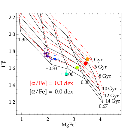
Figure 4: Index-index plot of MgFe’ and H$\beta$. On the left panels, the lines indicate the Thomas et al. (2011a) (TMJ) SSP model grid with Salpeter IMF, on the right panels the Vazdekis et al. (2015) MILES models with Salpeter IMF slope (unimodal $\Gamma_{\text{u}}$=1.3). The colored circle points indicate the index measurements, with red to blue color and decreasing symbol size denoting spectra from the center to the outer bins. We plot grids with two different values for [$\alpha$/Fe] (0.0 and 0.3 dex; and 0.0 and 0.4 dex, respectively) indicated by black solid and red dashed lines, which influences the age result. Also MILES models with different bimodal IMF result in different ages. For a fixed IMF, the models suggest a younger age for the center of NGC 3923 in the MgFe’ and H$\beta$ plane than at larger radi.

Figure 5: Same as Fig. 4, but for Mgb and Fe3. For each model set (TMJ on the left, MILES on the right, both with Salpeter IMF), we plot grids with three different ages, denoted by different lines (blue solid lines for 7.0 Gyr, black dashed for 9.0 Gyr, red dot-dashed for 11.0 Gyr). We tested also MILES models with different bimodal IMF $\Gamma_{\text{b}}$=0.3, 1.3, and 3.5 (not shown). All models, ages, and IMF slopes indicate a roughly constant [$\alpha$/Fe]$\sim$0.2 dex.

A common approach for estimating SSP parameters is to compare two spectral indices with a model grid. We have attempted to estimate the age with the spectral indices H$\beta$ and MgFe’=$\surd$(Mgb $\cdot$ (0.72$\cdot$ Fe5270 + 0.28$\cdot$Fe5335)) (Figure 4); and [$\alpha$/Fe] with Mgb and Fe3 = (Fe4383 + Fe5270 + Fe5335)/3 (Figure 5). We show the Thomas et al. (2011a, TMJ, see Appendix B for details) and MILES (Vazdekis et al., 2015) SSP model grids at our resolution of FWHM=14 Å. These two grids of SSP models have [$\alpha$/Fe] as parameter (unlike Conroy et al. 2018 SSP models). The TMJ models cover a larger range of metallicity, and have a finer sampling than the MILES models. Large, red and orange data points denote the central bins, green, cyan, and blue data points with decreasing size denote indices measured on the outer spectra.

The H$\beta$ - MgFe’ index-index plot, in combination with either model set, suggests a younger age for the center of NGC 3923 than at larger radii. The data points of the two central bins lie at isochrones for ages of $\sim$6 Gyr for TMJ models (left panel Fig. 4); the outer, emission-line corrected data points at $\sim$14 Gyr. We obtain a similar trend with the MILES SSP model grid (right panel), but several Gyr older ages. Both model sets use a Salpeter (1955) IMF. We note that H$\beta$ measurements that are not emission-corrected have as small values as H$\beta$=1.3 Å, and lie far below the extent of the model grids, at extremely old ages (>15 Gyr). This is unphysical and confirms our finding that Balmer emission line subtraction is required for the outer bins.

Carlsten et al. (2017) also studied the stellar populations of NGC 3923 out to 1 R_h, to measure age, metallicity, and [$\alpha$/Fe]. They used eight spectral indices (H$\beta$, Fe5015, Mg₁, Mg₂, Mg_b, Fe5270, Fe5335 and Fe5406), five of which overlap with ours, and the SSP models of Thomas et al. (2003). They also found younger ages in the center of NGC 3923 with spectral index fitting, but obtained older ages of about 10 Gyr with full-spectral fitting. Carlsten et al. (2017) explain this discrepancy with a higher sensitivity of index fitting to the presence of a young stellar sub-population compared to full-spectral fitting (see also Serra & Trager 2007).

To estimate the value of [$\alpha$/Fe], we compared our index measurements of Mgb and Fe3 (Fig. 5) with the TMJ (left) and MILES (right) models. All the measurements lie nearly parallel to the lines of constant [$\alpha$/Fe] (which have positive slope), between 0.0 and 0.3 dex. The SSP grids shown have ages of 7, 9, and 11 Gyr. We tested different ages (from 6-12 Gyr) and IMF slopes ($\Gamma_{\text{b}}$=0.3, 1.3, 3.5), and found a shift of the lines of constant metallicity (which have negative slope), but the lines of constant [$\alpha$/Fe] barely moved. We conclude that the nearly flat [$\alpha$/Fe]-profile derived from this plot is model- and age-independent. Moreover, the MILES SSP model grids with bottom-heavy to bottom-light IMF suggest the same constant [$\alpha$/Fe]-profile. We note also that the [$\alpha$/Fe] indicated by the Mgb-Fe3 plot is in agreement with the measurements of Carlsten et al. (2017). Their results scatter around [$\alpha$/Fe]=0.27 dex from $\sim$0.15 to 0.4 dex, with an almost flat [$\alpha$/Fe] profile.

All index-index plots indicate a metallicity gradient ranging from super-solar ([M/H]>0.4 dex) in the center to sub-solar ([M/H]<-0.3 dex) at 0.8 R${}_{\text{h}}$. The exact values depend on the assumed age.

We conclude that our [$\alpha$/Fe] estimate from index-index grids is well-determined: we obtain similar results when we use a different set of the SSP models, alter the stellar age by several Gyr, or modify the IMF slope. An alternative approach described in Section 4.1.3 also gives consistent values for [$\alpha$/Fe]. The age estimate from index-index plots is, however, sensitive to changes of [$\alpha$/Fe], and the H$\beta$ index lies even beyond the range of the MILES SSP models with a Kroupa (2001) IMF. We conclude that the index-index plots are not reliably able to constrain the stellar age of NGC 3923.

4.1.2 Age constraints with pPXF

In another attempt to constrain the stellar age and metallicity, we did not use spectral indices but rather full spectral fitting with pPXF in the wavelength region $\lambda$= 4000–5600 Å, which contains several age- and metallicity-sensitive Balmer and Fe lines. As mentioned in Sect. 3.3.1, pPXF assigns weights to the template model spectra, and the optimal template is a linear combination of all input models. This method allows the determination of a mass-weighted-mean age and metallicity, consisting of more than one stellar population. To determine age and metallicity, we used the program in a different manner than in Sect. 3.3.1, where we fit the LOSVD. The details are given in Appendix A.4. We did not include SSP models with all possible IMF values, but rather fit the spectra for each IMF slope value separately. We used the MILES SSP models (Vazdekis et al., 2015) with seven ages in the range of 2–14 Gyr, and nine metallicities at Z= $-$1.49, $-$1.26, $-$0.96, $-$0.66, $-$0.35, $-$0.25, 0.06, 0.15, and 0.26 dex. We considered SSP models with [$\alpha$/Fe]=0 dex and [$\alpha$/Fe]=0.4 dex in separate fits.

Figure 6: Age and metallicity fit results of NGC 3923 as a function of distance from the galaxy’s center, for the data at P.A.=0°, obtained with pPXF (Sect. 4.1.2) and Vazdekis et al. (2015) MILES models. Colors denote three different fixed IMF slopes $\Gamma_{\text{b}}$, in particular extremely bottom-light (black, $\Gamma_{\text{b}}$=0.3), Milky-Way-like (blue, $\Gamma_{\text{b}}$=1.3) and extremely bottom-heavy (red, $\Gamma_{\text{b}}$=3.5). Different symbols and lines denote models with different [$\alpha$/Fe], filled diamond symbols with solid lines are [$\alpha$/Fe]=0.0 dex, filled square symbols with dashed lines are [$\alpha$/Fe]=0.4 dex. Balmer emission-line correction was only required for the outer four spectra (filled symbols). Omitting the correction results in older ages (open symbols). Horizontal black lines in the lower panel show the spacing of the SSP models in metallicity space. While Z is rather robust, the age depends on [$\alpha$/Fe], $\Gamma_{\text{b}}$, and the emission-line correction.

Figure 7: Same as Fig. 6, but using the Conroy et al. (2018) models with solar abundances. Colors denote three different fixed IMF slopes, in particular extremely bottom-light (black, $x_{1}$=$x_{2}$=0.5), Salpeter-like (green, $x_{1}$=$x_{2}$=2.5) and extremely bottom-heavy (red, $x_{1}$=$x_{2}$=3.5). Horizontal black lines in the lower panel show the spacing of the SSP models in metallicity space.

We show our luminosity-weighted age and metallicity results as a function of radius in Fig. 6, age on the upper panel, metallicity on the lower panel. The results are shown with filled diamond symbols connected by solid lines for [$\alpha$/Fe]=0 dex, and filled square symbols, connected by dashed lines for [$\alpha$/Fe]=0.4 dex. Different colors denote different values for the IMF slope $\Gamma_{\text{b}}$. We show only the results for $\Gamma_{\text{b}}$=0.3, 1.3, and 3.5, but we fitted MILES models with all 14 possible bimodal IMF slopes individually.

The luminosity-weighted metallicity Z of the pPXF fit shows a significant gradient from +0.25 dex in the center to about -0.4 dex at the outermost bin at 1 R_h. The total metallicity is not strongly affected by different IMF slopes. The [$\alpha$/Fe]=0.4 dex SSP models have a higher metallicity Z, by 0.1–0.2 dex compared to the [$\alpha$/Fe]=0.0 dex models. The emission-line correction changes the metallicity values only slightly, by <0.04 dex.

Table 4: Absorption line index sets

Sect.	Used indices	Free parameters	Fixed	Symbols
4.1.3	Mgb	$Z_{\text{Mg}b}$	$t$, $\Gamma_{\text{b}}$, [X/H]=0
4.1.3	Fe4383, Fe5270, Fe5335	$Z_{\text{Fe}}$	$t$, $\Gamma_{\text{b}}$, [X/H]=0
4.2.2	MgFe’, TiO2, aTiO, bTiO (base set)	$t_{\text{p}}$, Z, $\Gamma_{\text{b}}$	[$\alpha$/Fe]=0.2	black x-symbols
4.2.2	MgFe’, TiO2, aTiO, bTiO, Ca4592	$t_{\text{p}}$, Z, $\Gamma_{\text{b}}$	[$\alpha$/Fe]=0.2	blue diamonds
4.2.2	MgFe’, TiO2, aTiO, bTiO, Fe5709	$t_{\text{p}}$, Z, $\Gamma_{\text{b}}$	[$\alpha$/Fe]=0.2	green triangles
4.2.2	MgFe’, TiO2, aTiO, bTiO, Fe5782	$t_{\text{p}}$, Z, $\Gamma_{\text{b}}$	[$\alpha$/Fe]=0.2	orange squares
4.2.2	MgFe’, TiO2, aTiO, bTiO, Ca4592, Fe5709, Fe5782	$t_{\text{p}}$, Z, $\Gamma_{\text{b}}$	[$\alpha$/Fe]=0.2	red asterisks
4.2.2	MgFe’, TiO2, aTiO, bTiO, Ca4592, Fe5709, Fe5782, Fe4531, Fe5406	$t_{\text{p}}$, Z, $\Gamma_{\text{b}}$	[$\alpha$/Fe]=0.2	cyan circles
4.2.4	MgFe’, TiO2, aTiO, bTiO, Ca4592, Fe5709, Fe5782	$t_{1}$, $t_{2}$, Z1, Z2, $w_{1/2}$, $\Gamma_{\text{b}}$	[$\alpha$/Fe]=0.2
4.2.4	MgFe’, TiO2, aTiO, bTiO, Ca4592, Fe5709, Fe5782, Fe4531, Fe5406	$t_{1}$, $t_{2}$, Z1, Z2, $w_{1/2}$, $\Gamma_{\text{b}}$	[$\alpha$/Fe]=0.2	cyan circles

Note. — age fitting with age prior: $t_{\text{p}}$ from Sect. 4.1.2; fixed [X/H]=0 means only solar abundances.

Our results for the stellar age are more complicated than the metallicity, as the age results depend strongly on our assumptions on the IMF slope, emission line correction, and a lesser degree the [$\alpha$/Fe] abundance. While the age difference between a bottom-light ($\Gamma_{\text{b}}$=0.3, black) and a Milky Way-like IMF ($\Gamma_{\text{b}}$=1.3, blue) is rather small, an increasingly bottom-heavy IMF ($\Gamma_{\text{b}}$=3.5, red) is several Gyr younger. The age difference between [$\alpha$/Fe]=0 dex and [$\alpha$/Fe]=0.4 dex ranges from +0.8 to -1.6 Gyr, but is negligible except for high values of $\Gamma_{b}$. We note that we applied the Balmer emission line correction derived in Sect. 3.3.1 for each of our fits. If we instead derived individual Balmer emission line corrections, using each set of model spectra, the age differences derived with [$\alpha$/Fe]=0 dex and [$\alpha$/Fe]=0.4 dex SSP models would be $\sim$1.5 Gyr in most of the outer spectra, irrespective of the assumed IMF slope.

We cannot test the pPXF fitting with the TMJ models, as we do not have the model spectra, only the model indices. But we applied the same fitting approach on a subset of the Conroy et al. (2018) models, all with solar abundances. The results are shown in Fig. 7 assuming three different IMF slopes ($x_{1}$=$x_{2}$=0.5, 2.5, or 3.5). Due to the different IMF slope definitions (Appendix B), it is not possible to make a quantitative comparison to the results obtained with MILES models. However, we would like to make a few general comments: (1) The outer four spatial bins indicate that Balmer emission line subtraction is needed, as found with MILES models; (2) for a more bottom heavy IMF-slope, the derived age is lower, as found with MILES models; (3) the age in the center is largest, and decreases with radius; however, the gradient is less significant compared to the MILES models; (4) there is a Z gradient, though it is offset to lower values than with the MILES models.

Overall, using pPXF we find an age gradient with oldest ages in the center. This is in contrast to the age estimate from the index-index grids, where the center is youngest (see Sect. 4.1.1). Carlsten et al. (2017) also analyzed data of NGC 3923 with both spectral indices and pPXF fitting. Like us, they found younger ages ($\sim$4 Gyr) with spectral indices, but older ages ($\sim$10 Gyr) with pPXF in the center of NGC 3923. This discrepancy may be caused by a young sub-population, which biases the Balmer-line-weighted age to the age of the young component, as found by Serra & Trager (2007). Depending on the age of the young component, this bias is important even though the mass-fraction of the young sub-population may be far less than 10 per cent. Also Carlsten et al. (2017) found that spectral indices are more sensitive to a young sub-population than full-spectral fitting. Full-spectral fitting appears to give a better estimate of the dominant, older stellar population. For this reason, we consider the pPXF age a better overall age estimate than the spectral index age.

Carlsten et al. (2017) fit their spectra of NGC 3923 with pPXF using the PEGASE-HR SSP models (Le Borgne et al., 2004) with a Salpeter IMF. In this case, they found a flat age profile close to 10 Gyr along major and minor axes, while we obtained a decreasing age with radius. A Salpeter IMF corresponds roughly to the case $x_{1}$=$x_{2}$=2.5 in the Conroy et al. (2018) models; and a more bottom-heavy IMF than $\Gamma_{\text{b}}$=1.3 in the MILES models (see Figs. 6 and 7). Carlsten et al. (2017) did not correct their outer spectra of NGC 3923 for Balmer emission, as we did. We tested omitting the Balmer emission correction and obtained increased best-fit ages by up to $\sim$1.3 Gyr in the outer bins, and thus a flatter age gradient (see open symbols in Fig. 6). This is closer to the results of Carlsten et al. (2017) and likely accounts for our different age profiles.

We note that there are several factors that influence our age estimate: (a) the IMF slope, (b) the emission-line correction, and (c) [$\alpha$/Fe]. In order to derive the IMF with spectral indices we make two assumptions which must be kept in mind when assessing the significance of any result: First, we use the emission line correction, because we found that it improves the full-spectral fit to SSP models in the outer bins (Sect. 3.3.1 and 4.1.1), and because omission causes a low H$\beta$ spectral index, which can only be explained by stellar ages >15 Gyr (Sect. 4.1.1). Second, as we constrained [$\alpha$/Fe] to be approximately 0.2 dex at all radii (Sect. 4.1.1 and  4.1.3), we linearly interpolated the pPXF output ages and MILES SSP model indices to [$\alpha$/Fe]=0.2 dex.

4.1.3 Estimation of [$\alpha$/Fe] with spectral-index fitting

We also applied the method described by La Barbera et al. (2013) to estimate [$\alpha$/Fe]. We compared the metallicity $Z_{\text{Mg}b}$ derived from Mgb with the metallicity $Z_{\text{Fe}}$ derived from Fe3. To obtain those metallicities, we fixed the IMF slope $\Gamma_{\text{b}}$ and age to certain values. We minimised $\chi^{2}$ following the equation

$$\chi^{2}(Z,\text{t})=\sum_{i}^{N}\left[\frac{(\text{EW}_{i}-\text{EW}_{\text{M},i}}{\sigma_{\text{EW}_{i}}}\right]^{2},$$ (1)

where EW_i denote measurements of the different absorption line indices, $\sigma_{\text{EW}}$ the respective uncertainties, and EW${}_{\text{M},i}$ the SSP model absorption-line indices at a given IMF slope $\Gamma_{\text{b}}$.

Using only the Mgb index we derived $Z_{\text{Mg}b}$; using Fe3 we derived $Z_{\text{Fe}}$, for each bin and spectrum. Vazdekis et al. (2015) showed that 0.59$\cdot(Z_{\text{Mg}b}-Z_{\text{Fe}})$ can be used as solar proxy of [$\alpha$/Fe], with an accuracy of 0.025 dex in [$\alpha$/Fe]. We applied the MILES SSP models (Vazdekis et al., 2015) with [$\alpha$/Fe]=0 dex, and interpolated the index measurements to a finer metallicity grid with spacing $\Delta$Z=0.02 dex. The high central Mgb index of our data made it necessary to extrapolate Mgb of the models up to Z=0.6 dex.

We present our results for the [$\alpha$/Fe] estimate in Fig. 8 as a function of radius. The profile is consistent with being constant to within the uncertainties. We derived [$\alpha$/Fe] for $\Gamma_{\text{b}}$=0.3, 1.3, and 3.5 and their respective best-fit ages derived in see Sect. 4.1.2 (black, blue, and red colored lines), and the differences are <0.04 dex. This is in agreement with La Barbera et al. (2016), who found that the variation of [$\alpha$/Fe] for different $\Gamma_{\text{b}}$ is at most 0.05 dex, which corresponds to more than two steps in our metallicity grid.

We compared our results to Thomas et al. (2005), who measured a higher value of [$\alpha$/Fe] in the central R_h/10 of NGC 3923 (0.3 dex, cyan triangle symbol). They used the indices H$\beta$, Mgb, and $\langle$Fe$\rangle$=0.5$\cdot$(Fe5270+ Fe5335) measured by Beuing et al. (2002) and the models from Thomas et al. (2003). When we use the Beuing et al. (2002) measurements of Mgb, Fe5270, and Fe5335 for the central bin, with our Fe4383 measurement and age measurement, we obtain a higher value of [$\alpha$/Fe]=0.28 dex in the center, and have better agreement with Thomas et al. (2005). This suggests that the different value for [$\alpha$/Fe] is mostly caused by differences of the data rather than the different method or models.

To investigate the effect of age, we derived [$\alpha$/Fe] with a fixed age of 14 Gyr (upper bound of our age grid, shown with orange triangles for the case $\Gamma_{\text{b}}$=1.3), and with an age that is 3 Gyr less than the best-fit age (green triangles for $\Gamma_{\text{b}}$=1.3). [$\alpha$/Fe] changes by no more than 0.04 dex. However, due to the deep Mgb line in the most central bin, the derived value of $Z_{\text{Mg}b}$ is at the upper bound of the grid (i.e. 0.6 dex), to compensate for the younger age (3 Gyr less than the best-fit age). This leads to a bias in [$\alpha$/Fe] to a lower value. If we force even younger ages, this bias affects also the second and third bins, and can lead to a drop of [$\alpha$/Fe] to $\sim$0.1 dex in the center. Apart from this bias effect in the center, a different age does not strongly influence [$\alpha$/Fe]. This method is consistent with our assumption of a constant [$\alpha$/Fe]=0.2, independent of the assumed IMF and age.

Figure 8: [$\alpha$/Fe] profile, measured from the relation [$\alpha$/Fe]=0.59$\times(Z_{\text{Mg}b}-Z_{\text{Fe}})$ (Vazdekis et al., 2015), derived with $\Gamma_{\text{b}}$=0.3, 1.3, and 3.5 (black, blue, and red colored lines); for a higher age of 14 Gyr at all radii (orange triangles), or a lower age (3 Gyr less than the best-fit age of Sect. 4.1.2, green triangles). The black error bar at the upper right denotes the typical uncertainty of this method. The central value of Thomas et al. (2005) is a downward-facing cyan triangle, and Carlsten et al. (2017) a purple square symbol.

4.2 IMF measurement

In this section we use spectral indices to estimate the IMF slope of NGC 3923 (in Sect. 5, we present our results for full spectral fitting). First, we explain our method (Sect. 4.2.1); then we explore using different sets of spectral indices, fitting parameters (listed in Table 4), and SSP models for a single stellar population (Sect. 4.2.2). Then, we test the effect of taking non-solar abundances into account, and explore which combination of indices and fitting parameters is most accurate and precise using simulated spectra (Sect. 4.2.3).

Since the evolutionary history of a galaxy may not necessarily be described by a simple, single age, but more likely a distribution of ages, we also explore the effects of fitting combinations of two stellar populations (Sect. 4.2.4).

4.2.1 Method

To fit the IMF, we minimized the expression (see Martín-Navarro et al., 2015a)

$$\begin{aligned} \chi^{2}(\Gamma_{\text{b}},\text{Z},[\text{X/H}],t)=\left[\frac{t(\Gamma_{\text{b}})-t_{\text{M}}}{\sigma_{\text{t}}/\sqrt{N}}\right]^{2}\\ +\sum_{i}^{N}\left[\frac{\text{EW}_{i}-(\text{EW}_{\text{M},i}+\sum_{\text{X}}\Delta_{\text{X,}i}\cdot[\text{X/H}])}{\sigma_{\text{EW}_{i}}}\right]^{2},\end{aligned}$$ (2)

where EW_i denotes the data absorption-line indices, $\sigma_{\text{EW}}$ the uncertainty of the measured spectral indices, EW${}_{\text{M},i}$ the SSP model indices, and $\Delta_{\text{X,}i}$ the correction of the line strength for a non-solar elemental abundance.

The first term is used to set a prior on the age measurement. We used $\Gamma_{\text{b}}$-dependent luminosity-weighted ages $t$($\Gamma_{\text{b}}$) as measured in Sect. 4.1.2. We linearly interpolated our measurements at [$\alpha$/Fe]=0.0 dex and 0.4 dex to [$\alpha$/Fe]=0.2 dex. $\sigma_{\text{t}}$ is the quadratic sum of the standard deviation of the two measurements (at [$\alpha$/Fe]=0.0 dex and [$\alpha$/Fe]=0.4 dex), and the width of a Gaussian fit to the age distributions (Sect. 4.1.2), $t_{\text{M}}$ is the age of a SSP model. As in Martín-Navarro et al. (2015a), we re-scale $\sigma_{\text{t}}$ by dividing it by the square root of the number of indices $N$. This term biases the age estimate of the $\chi^{2}$ minimization to our results from Sect. 4.1.2, and helps to break the degeneracy when using spectral indices that are both age- and IMF-sensitive.

The second term contains the non-solar abundance corrections $\Delta_{\text{X,}i}$, which are used when we include any elemental abundances [X/H] as fitting parameters, or fix the value of any elemental abundance. We derived the non-solar abundance correction $\Delta_{\text{X,}i}$ from the model spectra of Conroy et al. (2018) with a Kroupa IMF, and for a range of elemental abundance variations. For a finer sampling, we inter- and extrapolated the index measurements in steps of 0.1 dex to the range $-$0.4 dex to +0.4 dex for [Ti/H] and [Fe/H] (original sampling was $-$0.3, 0.0, +0.3 dex); $-$0.3 dex to +0.3 dex for [C/H] (original $-$0.15, 0.0, +0.15 dex); 0 dex to +1.0 dex for [Na/H] (original $-$0.3, 0.0, 0.3, 0.6, 0.9 dex) and 0 dex to +0.4 dex for [O/H] (original 0.0, 0.3 dex). We assume that the response of the indices to a single element is linear, and independent of other elemental variations, as is commonly assumed (Sansom et al., 2013; Alton et al., 2017; Vaughan et al., 2018a; Parikh et al., 2018). We computed the correction $\Delta_{\text{X,}i}$ of each absorption-line index to the variation of a given chemical elemental abundance

$$\begin{aligned} \Delta_{\text{X,}i}=\frac{\text{EW}_{\text{M,}i\text{,[X/H]}=0}-\text{EW}_{\text{M,}i\text{[X/H]}\neq\,0}}{\delta([\text{X/H}])},\end{aligned}$$ (3)

where $\text{EW}_{\text{M,}i\text{,[X/H]}=0}$ is the index measured on the reference model spectrum with solar abundances, and $\text{EW}_{\text{M,}i\text{[X/H]}\neq\,0}$ is the index measured on a model spectrum with a variation of one single element [X/H].

We minimized Eq. 2 using two different sets of models for the EW${}_{\text{M},i}$: (1) Conroy et al. (2018) models and (2) MILES models (Vazdekis et al., 2015). The former Conroy models have ages ranging from 1-13.5 Gyr, and Z from $-1.0$ to 0.2 dex, interpolated to steps of 0.1 dex. As we previously derived [$\alpha$/Fe]=0.2 dex for our data using the Mgb index, we use the non-solar abundance correction for [Mg/H]=0.2 dex to all Conroy model indices. The latter MILES models have $t_{\text{M}}$ = 1–14 Gyr and Z = $-$0.7 dex to +0.26 dex. We interpolated the index measurements for a finer metallicity sampling with $\Delta$Z = 0.05 dex. To account for the supersolar [$\alpha$/Fe], we tested two approaches: We interpolated the MILES model indices with [$\alpha$/Fe]=0.0 and 0.4 dex to [$\alpha$/Fe]=0.2 dex, or we used the non-solar abundance correction for [Mg/H]=0.2 dex, as for Conroy model fits.

In a subset of fits, we fit two stellar populations (2SPs) instead of one single stellar population using MILES models only. In order to obtain the spectral indices of 2SPs, we combined two of the MILES models with different ages, metallicities, but the same [$\alpha$/Fe] and $\Gamma_{\text{b}}$. Two SSP models were combined with weights $w_{1/2}$ = 0.0/1.0, 0.25/0.75, 0.5/0.5, or 0.75/0.25, before we measured the spectral indices on the 2SP models. We did this for [$\alpha$/Fe]=0 dex and [$\alpha$/Fe]=0.4 dex, and interpolated our index measurements to [$\alpha$/Fe]=0.2 dex. For the 2SP fit, the age prior was set such that it constrained the weighted mean age of the two stellar populations, as detailed further in Sect. 4.2.4.

We determined the best-fit parameter values as follows: We transformed our $\chi^{2}$ from Equ. 2 to the likelihood $L$=$exp(-(\chi^{2}-min(\chi^{2}))/2)$, divide $L$ by the sum of all $L$, and marginalize over each fitting parameter. We calculated the best fit value by taking the weighted mean of each parameter, weighted by the marginalized likelihood. The fitting uncertainties are determined from the range of models within the 1-$\sigma$ confidence limit, which is calculated for the respective degree of freedom of each fit.

4.2.2 Results for one single stellar population

Figure 9: Results of spectral index fitting for different index subsets, fitting stellar age (top panel), metallicity Z (center panel), and IMF slope $\Gamma_{\text{b}}$ (bottom panel), using MILES models interpolated to [$\alpha$/Fe]=0.2 dex. The horizontal dashed line denotes a Milky Way-like Kroupa IMF. Different colored symbols denote different index subsets, as listed in Table 4.

Figure 10: Results of spectral index fitting, including [O/H], [C/H], and [Na/H] as fitting parameters. We used the MILES models interpolated to [$\alpha$/Fe]=0.2 dex (left panel); the MILES models with [$\alpha$/Fe]=0 dex, but with a fixed abundance correction [Mg/H]=0.2 dex (middle panel); Conroy models with a fixed abundance correction [Mg/H]=0.2 dex (right panel). Note the different IMF parameterization with $\Gamma_{\text{b}}$ (left and central panel with MILES models; $dN/d\log{m}\propto m^{-\Gamma_{b}}$); or $x_{1}$ and $x_{2}$ (right panel with Conroy models; $dN/dm\propto m^{-x_{i}}$), the lower horizontal dashed line denotes a Milky Way-like Kroupa IMF ($x_{1}$=1.3; $x_{2}$=2.3); the dashed lines shown at $x_{1}$=$x_{2}$=2.3 denote a Salpeter IMF slope. Different colored symbols denote different index subsets, as listed in Table 4.

Assuming a single stellar population, we fit the bimodal IMF slope $\Gamma_{\text{b}}$, stellar metallicity Z, and age $t$ with an age prior, which is a function of $\Gamma_{\text{b}}$. We tried different sets of spectral indices:

Our base set of spectral indices are: MgFe’, TiO₂, aTiO, and bTiO. This is similar to the set used by La Barbera et al. (2016). They used Mg4780 instead of bTiO, but the index definitions are almost identical. Further, La Barbera et al. (2016) used TiO₁, which is unavailable to us because of IMACS chip gaps. We measured the spectral indices on the MILES models and investigated their sensitivity to different stellar population parameters. MgFe’ is a strong metallicity indicator (Thomas et al., 2003), while TiO₂, aTiO, and bTiO are sensitive to the IMF, increasing with a larger fraction of low-mass stars (see also Fig. 17 top row). This is consistent with the results of Spiniello et al. (2014), using different stellar population models. We decided to include also IMF-sensitive indices that decrease with a larger fraction of low-mass stars, and are sensitive to the same abundances. In particular, we tested including the indices Ca4592, Fe5709, and Fe5782 (Fig. 17 bottom row). In another set we added the indices Fe4531 and Fe5406. They are mostly sensitive to age, and Z, but not IMF slope.

There are other prominent indices that we were unable to use for a variety of different reasons: NaD (5900 Å) and the near-infrared Ca Triplet lines (8400–8800 Å) fall partially on chip gaps; Na I (8190 Å) was observed with a shorter exposure time and has therefore lower S/N, causing large uncertainties compared to other indices, Na I therefore provides no constraining power; the bluer Ca H+K (3900–4000 Å) region is potentially affected by H$\epsilon$ Balmer emission, and more sensitive than other spectral regions to a complex star formation history (Kacharov et al., 2018), which can cause large discrepancies for SSP models. Further, if we included the Ca H+K index, we also would have to include [Ca/Fe] as additional fitting parameter. The degree-of-freedom of our fit would remain the same and our ability to constrain the IMF would not improve.

Our fit results using MILES models with constant [$\alpha$/Fe] = 0.2 dex are shown in Fig. 9, different symbols denote the different index combinations, as listed in Table 4. The result for the age (upper panel) is rather stable for different index combinations, due to the age prior, but for some bins the age results have a standard deviation of up to 0.7 Gyr.

The metallicity (middle panel) is less dependent on the index set, while the IMF slope (bottom panel) is affected by the selection of indices. The standard deviation of $\Gamma_{\text{b}}$ ranges over 0–0.8 per bin. There are some outliers, in particular at the third and fifth radial bins (6.9 and 32.4″), but the overall trend is an extremely bottom-heavy IMF in the center, while the outer bins are consistent with a Kroupa IMF ($\Gamma_{\text{b}}$=1.3). The outliers are the fits with the base set (MgFe’, TiO₂, aTiO, and bTiO, black x-symbols), the Ca4592-set (blue diamonds), and the Fe5782-set (orange squares). Increasing the number of indices produces a smoother IMF gradient, and decreases the uncertainties. We note that a higher age result is usually compensated by a lower IMF slope and vice versa.

For the two central bins the best-fit results of all index sets are at or close to the upper bounds of the models, for all parameters. This may be related to the fact that the MILES models are not able to match the MgFe’ and several other metallicity-sensitive spectral indices in the two central bins, but have large residuals ($\sim$8–26$\sigma$). As models with higher metallicity are not reliable to use, we had to limit Z to <0.3 dex, which is compensated by higher ages. We conclude that the uncertainties for our central data points, though formally low, are underestimated.

In addition, we used MILES models with [$\alpha$/Fe]=0 dex and an elemental abundance correction for [Mg/H]=0.2 dex instead. This results in slightly lower values for Z (by <0.1 dex), and higher values for $\Gamma_{\text{b}}$ (by 0.1 to 0.8 dex), especially at large radii. Overall, the Z gradient is steeper, and the $\Gamma_{\text{b}}$ gradient is shallower. The differences compared to Fig. 9 are within the ranges of the uncertainties, but, in most cases, the fits obtain a smaller $\chi^{2}$ than the [$\alpha$/Fe]=0.2 dex models.

To investigate the age-IMF dependency, we repeated our fits with fixed ages. We fixed the stellar ages to the best-fit pPXF value obtained for a Milky Way-like Kroupa IMF ($\Gamma_{\text{b}}$=1.3). As a consequence, the scatter of $\Gamma_{\text{b}}$ for different index combinations decreases, although there are still some outliers. All changes are within or close to the uncertainties compared to the case where we fit the ages. To further test the influence of the stellar age on the results, we fixed the age to 8, 11, and 14 Gyr. We found that higher ages result in lower values of the IMF slope. The changes range from 0 to 1.3 dex of $\Gamma_{\text{b}}$ per 3 Gyr change. This means that age and IMF slope are anti-correlated.

In general, when we fit the age and IMF together, we marginalize over all fitting parameters. This takes the age-IMF degeneracy into account, and causes large uncertainties. When we fix the age, the IMF uncertainties are underestimated, as they do not contain the uncertainty caused by the IMF-age degeneracy. However, as fixing the age to the $\Gamma_{\text{b}}$=1.3 derived value changes the IMF by <1$\sigma$, we fix the age in the following section, and introduce elemental abundances as fitting parameters.

4.2.3 Results for one single stellar population with element-abundance fit

In this section we repeated the spectral index fits, and added elemental abundances as fitting parameters, as the selected indices are sensitive to variations of [O/H], [C/H], [Ti/H], [Na/H], or [Fe/H]. We did not fit the base set with abundance parameters, as the degree of freedom of the fit would be zero.

We ran simulations with mock spectra to test whether we are able to constrain the stellar populations with our sets of indices and elemental abundances. We constructed mock spectra with a Kroupa and a bottom-heavy IMF slope, using Conroy models. The details are described in Appendix D.1. The main results are as follows: The low-mass IMF slope $x_{1}$ (0.08–0.5 $M_{\sun}$) can hardly be constrained, and tends to be overestimated relative to the input values (by up to 2 dex). The higher mass slope $x_{2}$ (0.5–1.0 $M_{\sun}$) is better constrained, especially with the Fe5709 and the combined index sets, though $x_{2}$ tends to be underestimated (by up to 2 dex). The most accurate results for age, Z and $x_{2}$ are obtained when the abundances [Na/H], [O/H] and [C/H] are also fit, though [O/H] and [C/H] are underestimated, and $x_{1}$ overestimated (Fig. 18, lower right panel).

We fit these index and abundance sets for both MILES and Conroy models. As the index fitting has only a small degree of freedom, we fixed the age to the values of Sect. 4.1.2 for $\Gamma_{\text{b}}$=1.3, corresponding to Kroupa IMF. The results are shown in Fig. 10, left panel for MILES models with [$\alpha$/Fe]=0.2 dex, middle panel for MILES models with [Mg/H]=0.2 dex, and right panel for Conroy models with [Mg/H]=0.2 dex. For all cases the metallicity Z has a gradient, but the values are lower by $\sim$0.3 dex for the Conroy models for the outer bins. There is disagreement for [Na/H], [O/H] and [C/H] in the central bins between the SSP model sets, and the abundances have large uncertainties at large radii. We conclude that we are not able to unambiguously constrain the considered elemental abundances [Na/H], [O/H], and [C/H] with our optical spectral index fits for NGC 3923. Although this fitting set-up works best for simulations, it has large uncertainties for our data, and barely constrains the IMF slope.

Figure 11: Results of spectral index fitting with a linear combination of two stellar populations of MILES models, fitting stellar ages (with age prior on weighted mean age), metallicities Z, and a common IMF slope $\Gamma_{\text{b}}$. The horizontal dashed line denotes a Milky Way-like Kroupa IMF. Cyan circle symbols denote the weighted mean of age and metallicity, red triangles and blue squares denote the two different stellar populations.

4.2.4 Results for two stellar populations

We used linear combinations of two MILES SSP models to fit the IMF slope $\Gamma_{\text{b}}$ with two stellar populations. Because of the large number of fitting parameters ($\Gamma_{\text{b}}$, two ages $t_{1}$, $t_{2}$, two metallicities Z₁, Z₂, weights $w_{1/2}$), we used only the index set with the largest number of indices (see Table 4), and did not fit stellar abundances. In this toy model we assumed that both populations have the same [$\alpha$/Fe]=0.2 and $\Gamma_{\text{b}}$, which is not necessarily true. We set the age prior on the weighted mean age, i.e. on $t_{\text{M}}=w_{1/2}\cdot t_{1}+(1-w_{1/2})\cdot t_{2}$. Our stellar population results are shown in Fig. 11. The weighted mean ages and metallicities (cyan circles) are a linear combination of two stellar populations, shown as red triangles and blue squares. Unexpectedly, our best fit consists of a younger, more metal-poor population, and an older, more metal-rich population, which contributes the larger weight in most spectral bins. The fact that the younger population is more metal-poor than the older population suggests that either this simplified model is wrong or, perhaps that the young and old stellar populations formed in different environments, and were mixed later. In any case, these results underscore the fact that the results in such analyses depend on initial assumptions about the (unknown) star formation history of galaxies. As NGC 3923 is a shell galaxy, it may have an unusual star formation history.

In comparison with the fit of only one stellar population and the same index subset, the weighted mean metallicity in the outer five bins is higher by up to 0.17 dex. The central two bins do not require a second stellar population, and we find the same result as for the 1SP fit. The IMF slope is bottom-heavy reaching a maximum value of $\Gamma_{\text{b}}$=3.5 in the center, and decreasing to 1.2–2.0 in the outer bins. In the outer four bins $\Gamma_{\text{b}}$ is higher than for the 1SP fit, though the measurements are in agreement within their uncertainties.

5 Full spectral-fitting analysis

Using the full information of a spectrum rather than single measurements on selected spectral regions has the advantage that all available information is used. The number of free parameters is given by the number of pixels in the spectrum rather than the number of spectral indices. This allows a fit to a larger number of stellar population parameters simultaneously, and the opportunity to understand how they influence each other. Also Conroy & van Dokkum (2012b), Podorvanyuk et al. (2013), van Dokkum et al. (2017), and Vaughan et al. (2018b) used full spectral fitting to constrain the IMF. In this section we describe our method (Sect. 5.1), illustrate our results (Sect. 5.2), and discuss degenerate solutions and parameter correlations (Sect. 5.3).

Table 5: PyStaff fit sets

Sect.	Wavelength range [Å]	Free parameters	Fig.	Symbols
5.2	4285–4421, 4504–4629, 4744–4893, 5144–	$x_{1}$, $x_{2}$, $t$, Z, Balmer, [Mg/H],	20a	green circles
	5657, 5674–5738, 5767–5813, 6068–6417	[Fe/H], [Ti/H], [O/H], [C/H]
5.2	4285–4421, 4504–4629, 4744–4893, 5144–	$x_{1}$, $x_{2}$, $t$, Z, Balmer, [Mg/H],	20b	blue squares
	5657, 5674–5738, 5767–5813, 6068–6417	[Fe/H], [Ti/H], [O/H], [C/H]
		[Na/H], [Ca/H], [N/H], [Si/H]
5.2	4285–4421, 4504–4629, 4744–4893, 5144–	$x_{1}$, $x_{2}$, $t$, Z, Balmer, [Mg/H],	21c	orange diamonds
	5657, 5674–5738, 5767–5813, 5885–6417	[Fe/H], [Ti/H], [O/H], [C/H]
		[Na/H], [Ca/H], [N/H], [Si/H]
5.2	4285–4421, 4504–4629, 4744–4893, 5144–	$x_{1}$, $x_{2}$, $t$, Z, Balmer, [Mg/H],	21d	red triangles
	5657, 5674–5738, 5767–5813, 5885–6417,	[Fe/H], [Ti/H], [O/H], [C/H]
	8164–8244, 8474–8524	[Na/H], [Ca/H], [N/H], [Si/H]

5.1 Method

We use the python package PyStaff (Python Stellar Absorption Feature Fitting) developed by Vaughan et al. (2018b), implementing some of the features of pPXF, and the SSP models of Conroy et al. (2018). We fit stellar age [1, 14 Gyr], Z [-1.5, 0.3 dex], the two IMF slopes [0.5, 3.5], and nine abundances, Na [$-0.45$, 1.0 dex], Ca [$-0.45$, 0.45 dex], Fe [$-0.45$, 0.45 dex], C [$-0.2$, 0.2 dex], N [$-0.45$, 0.45 dex], Ti [$-0.45$, 0.45 dex], Mg [$-0.45$, 0.45 dex], Si [$-0.45$, 0.45 dex], and O (=O, Ne, S) [0, 0.45 dex]. We tested including more elemental abundances (e.g. [Cr/H], [Ba/H], [Sr/H]) to improve our fit results, but without noticeable effects.

We included gas emission line templates to fit the Balmer lines, which were tied to the same kinematics and fixed the relative fluxes (H$\gamma$=0.47$\times$H$\beta$, Oh et al., 2011). We had thus three additional fitting parameters: the gas emission line flux, gas velocities and gas velocity dispersion. In agreement with the pPXF fits, we found that the Balmer emission line correction is negligible in the central bins, but becomes important at larger radii.

To speed up the fit, we resampled all spectra to a 1.25 Å-spaced wavelength grid. We also converted from air to vacuum wavelengths, in which the SSP models are computed. PyStaff models the spectral continuum with polynomial functions in four distinctive wavelength ranges. Besides the chip gaps, we excluded bad pixel regions from the fit.

The PyStaff code uses the Markov-chain Monte-Carlo (MCMC) package emcee (Foreman-Mackey et al., 2013). We explored the large parameter space with 100 walkers and 8,000 steps. In addition, we did one test run with 200 walkers and 100,000 steps, and obtained consistent results.

For an easier comparison with the spectral index fitting, we fit a wavelength region that corresponds to the spectral indices used in Sect. 4.2.2 with the combined index set, and in addition the H$\gamma$ and H$\beta$ regions. The fit included the spectral regions of H$\gamma_{A}$, Fe4531, bTiO, H$\beta$, Mgb, Fe5270, Fe5335, Fe5406, aTiO, Fe5709, Fe5782, and TiO₂ indices (see Table 5 for exact wavelength range); results are denoted as blue square symbols in Fig. 12. To improve the [Na/H] estimate we included the red parts of the NaD and TiO₁ features (denoted as orange diamond symbols in Fig. 12. We further added the near-infrared spectra, which include NaI (8190 Å) and part of the Ca1 (8500 Å) feature (red triangle symbols in Fig. 12). At shorter wavelengths ($\sim$3760–4190,Å) our spectra are noisier (see also Fig. 2), and the fit residuals are larger. It is possible that the discrepancy between models and data is caused by a complex star formation history, to which this wavelength region is more sensitive (Kacharov et al., 2018). To prevent potential biases, we excluded wavelengths <4200 Å from our fit. As before, we tested our fitting set-ups in simulations as described in Appendix D.2.

We also fit the central four spectra that are at a P.A.=48° offset from the major axis, to test the influence of a slightly different wavelength region. We obtained consistent results in most cases, with only small differences for Z, [N/H], and [Ca/H]. We conclude that the small difference in the fit wavelength range due to the different chip gaps is negligible.

5.2 Stellar population results

The best-fit stellar age based on PyStaff has a gradient of $\sim$10 to 7 Gyr, and is several Gyr younger than the ages obtained in Sect. 4, based on fitting MILES models, where we found a gradient ranging from $\sim$14 to 10 Gyr. For the metallicity we obtained a decreasing profile, with about Z$\lesssim$0.2 dex in the center, decreasing to -0.4 dex at the outermost bin, similar to our index fitting results with MILES models, but higher than obtained with index fitting using Conroy models. [Mg/H] reaches $\sim$0.22 dex in the center, decreasing to 0.12 dex at 54 arcsec. We used the Mgb index and thus Mg as [$\alpha$/Fe] tracer in Sect. 4.1.1 and 4.1.3 with MILES and TMJ models, and found values ranging from 0.25 to 0.19 dex. In Sect. 4.2.3 we assumed that these parameters correspond to each other, and indeed, our result for [Mg/H] is roughly consistent with our result for [$\alpha$/Fe].

The IMF results based on PyStaff full spectral fitting differ from our spectral index fitting results. $x_{1}$ is close to a Kroupa IMF slope and constant as a function of radius; however, as for spectral index fitting, $x_{1}$ is not well constrained. On the other hand, we obtain a bottom-heavy $x_{2}$. Though, the measurement uncertainties are large enough that a Kroupa IMF slope is only excluded by 1.3 $\sigma$ (1.8 $\sigma$ with near-infrared data) in the central two bins, but by more than 2.5 $\sigma$ (2.7 $\sigma$) in the radial bins centered at 6.9 and 16.2 arcsec. There is no clear gradient for $x_{2}$; at all radial bins $x_{2}$ is consistent with a value of 2.9 within 1 $\sigma$ (see also Table 6).

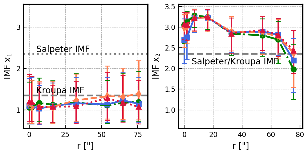
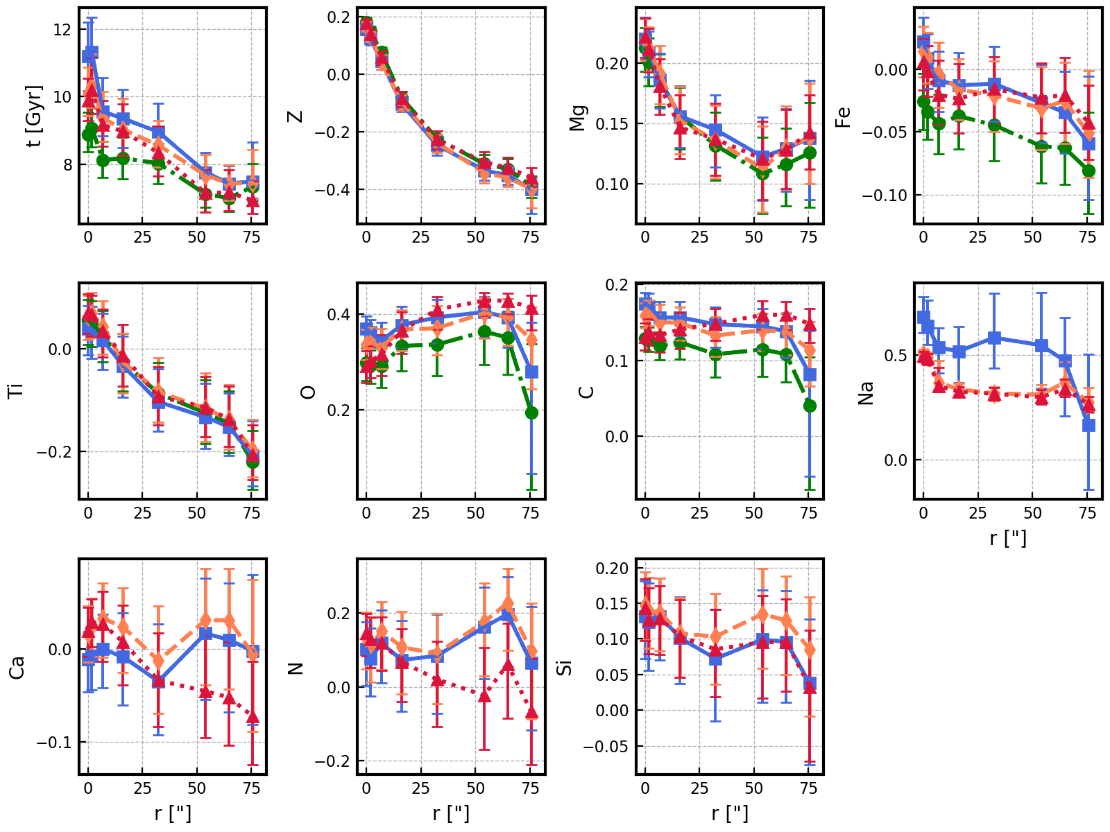
Figure 12: Stellar population gradients obtained with Pystaff fit for NGC 3923. The different colors denote different fitting set-ups, as listed in Table 5. The panels show as a function of radius $r$ in arcsec along the major axis, from left to right and top to bottom: IMF slopes $x_{1}$ (0.08-0.5 $M_{\sun}$), and $x_{2}$ (0.5-1.0 $M_{\sun}$), where the grey dashed horizontal line marks the Kroupa (2001) IMF, the dotted line at $x_{1}$ marks the Salpeter (1955) IMF; stellar age in Gyr; metallicity Z; elemental abundances [Mg/H], [Fe/H], [Ti/H], [O/H], [C/H], [Na/H], [Ca/H], [N/H], [Si/H].

As in Sect. 4.2.3, we tested how the results change when considering different abundances in the fit. For example, we fit our data with only five abundances (green circle symbols in Fig. 12, details listed in Table 5) instead of nine abundance parameters. This decreases the age in the central bins by 1 Gyr. Also the results for several elemental abundances are influenced. We compared the best-fit model spectra to our data and found that the 5-abundance best-fit model has larger fit residuals than the 9-abundance best-fit model in the masked wavelength region 4629–4744 Å (see also Fig. 20). We also ran fits of simulated mock spectra (see Appendix D.2 for details), and found that, indeed, ignoring the abundances [Na/H], [N/H], [Ca/H], and [Si/H] in a 5-abundance fit leads to less accurate results for age, Z, [Fe/H], and [O/H]. We conclude that it is important to add all nine tested elemental abundances in the full spectral fit in order to constrain the stellar populations of NGC 3923.

5.3 Degeneracies, correlations, and biases

As is well known, several fitting parameters are correlated. We inspected the probability distribution functions (PDF) of our fits and found the following correlations: Age-metallicity anti-correlation, $x_{2}$-age anti-correlation, $x_{2}$-O anti-correlation, O-C correlation, C-Fe correlation, and Mg-Fe correlations. The $x_{1}$ PDF is peaked at the lower bound at most bins, the $x_{2}$ PDF at the upper bound in the third and fourth bin. Also [O/H] peaks at the upper bound in some fits. Overall, the PDFs in the fits with and without the near-infrared wavelength range are very similar, except that the uncertainties are smaller when we include the near-infrared data (see also Table 6).

We used simulations of mock spectra to discover potential biases on our fitting parameters, and evaluate the accuracy and precision of our results (Appendix D.2). Using our preferred optical fitting set-up, with 9 abundance parameters and including the NaD absorption line region, our simulations found accurate results (meaning in agreement with the input value within the uncertainties) for age, Z, $x_{1}$, $x_{2}$, [Fe/H], [Ti/H], [O/H], [Ca/H], [N/H], and [Si/H]. [Mg/Fe] and [Na/Fe] are slightly overestimated (by $\textless$ 0.01 dex), [C/Fe] can be slightly underestimated. Interestingly, our simulation of optical spectra show that a bottom-heavy IMF slope can be measured with a higher precision than a Kroupa IMF. The uncertainty for a Kroupa IMF compared to a bottom-heavy IMF is greater by a factor 2.6 for $x_{1}$, and by a factor 2.2 for $x_{2}$. For galaxies with a bottom-heavy IMF in the center and a Kroupa-like IMF at larger radii, this complicates the IMF gradient measurement.

To test possible improvements to our analysis, we added the near-infrared spectral features NaI (8200 Å) and the first Ca Triplet line ($\sim$8500 Å). The near-infrared data does not influence our results of NGC 3923 significantly, but the uncertainties of the IMF measurements are decreased (see Table 6). Also our simulations show that near-infrared data significantly improve the precision of $x_{1}$ and $x_{2}$.

Table 6: PyStaff fit results

r [arcsec]	0.0	1.847	6.9	16.2	32.4	54.0	64.8	75.6
r/$R_{h}$	0.0	0.02	0.08	0.1875	0.375	0.625	0.75	0.875
preferred optical fit
$x_{1}$	$1.1^{+0.7}_{-0.5}$	$1.1^{+0.6}_{-0.4}$	$1.1^{+0.6}_{-0.4}$	$1.1^{+0.6}_{-0.4}$	$1.2^{+0.6}_{-0.5}$	$1.3^{+0.7}_{-0.6}$	$1.3^{+0.7}_{-0.5}$	$1.4^{+0.8}_{-0.6}$
$x_{2}$	$3.0^{+0.3}_{-0.5}$	$3.0^{+0.3}_{-0.4}$	$3.2^{+0.2}_{-0.3}$	$3.2^{+0.2}_{-0.3}$	$2.9^{+0.4}_{-0.5}$	$2.9^{+0.4}_{-0.5}$	$2.8^{+0.4}_{-0.5}$	$2.4^{+0.6}_{-0.8}$
t [Gyr]	$10.1^{+0.8}_{-0.7}$	$10.3^{+0.9}_{-0.6}$	$9.4^{+0.8}_{-0.7}$	$9.0^{+0.9}_{-0.8}$	$8.6^{+0.7}_{-0.7}$	$7.7^{+0.6}_{-0.5}$	$7.4^{+0.5}_{-0.5}$	$7.4^{+1.0}_{-0.5}$
Z	$0.17^{+0.02}_{-0.02}$	$0.13^{+0.02}_{-0.02}$	$0.04^{+0.02}_{-0.03}$	$-0.10^{+0.03}_{-0.03}$	$-0.24^{+0.03}_{-0.03}$	$-0.34^{+0.03}_{-0.04}$	$-0.36^{+0.04}_{-0.03}$	$-0.40^{+0.03}_{-0.07}$
Mg	$0.22^{+0.02}_{-0.02}$	$0.21^{+0.02}_{-0.02}$	$0.19^{+0.02}_{-0.03}$	$0.15^{+0.03}_{-0.03}$	$0.14^{+0.03}_{-0.03}$	$0.11^{+0.04}_{-0.04}$	$0.13^{+0.03}_{-0.03}$	$0.14^{+0.04}_{-0.04}$
Fe	$0.01^{+0.02}_{-0.02}$	$0.01^{+0.02}_{-0.02}$	$-0.00^{+0.03}_{-0.03}$	$-0.02^{+0.02}_{-0.02}$	$-0.02^{+0.03}_{-0.03}$	$-0.03^{+0.03}_{-0.03}$	$-0.03^{+0.03}_{-0.03}$	$-0.05^{+0.05}_{-0.04}$
Ti	$0.06^{+0.04}_{-0.05}$	$0.07^{+0.04}_{-0.05}$	$0.04^{+0.05}_{-0.05}$	$-0.03^{+0.06}_{-0.06}$	$-0.08^{+0.07}_{-0.06}$	$-0.12^{+0.07}_{-0.06}$	$-0.14^{+0.07}_{-0.06}$	$-0.20^{+0.06}_{-0.05}$
O	$0.34^{+0.03}_{-0.03}$	$0.34^{+0.03}_{-0.03}$	$0.33^{+0.04}_{-0.04}$	$0.37^{+0.04}_{-0.04}$	$0.37^{+0.05}_{-0.06}$	$0.40^{+0.03}_{-0.05}$	$0.39^{+0.04}_{-0.06}$	$0.35^{+0.07}_{-0.10}$
C	$0.16^{+0.02}_{-0.02}$	$0.16^{+0.02}_{-0.02}$	$0.15^{+0.02}_{-0.02}$	$0.15^{+0.02}_{-0.02}$	$0.13^{+0.02}_{-0.03}$	$0.14^{+0.02}_{-0.03}$	$0.14^{+0.02}_{-0.03}$	$0.11^{+0.04}_{-0.05}$
Na	$0.50^{+0.02}_{-0.03}$	$0.49^{+0.02}_{-0.04}$	$0.37^{+0.10}_{-0.03}$	$0.34^{+0.03}_{-0.02}$	$0.32^{+0.03}_{-0.03}$	$0.31^{+0.05}_{-0.04}$	$0.37^{+0.10}_{-0.05}$	$0.27^{+0.07}_{-0.05}$
Ca	$0.02^{+0.03}_{-0.03}$	$0.02^{+0.03}_{-0.03}$	$0.03^{+0.04}_{-0.04}$	$0.02^{+0.04}_{-0.05}$	$-0.01^{+0.06}_{-0.06}$	$0.03^{+0.06}_{-0.07}$	$0.03^{+0.06}_{-0.07}$	$-0.00^{+0.08}_{-0.08}$
N	$0.13^{+0.07}_{-0.08}$	$0.11^{+0.08}_{-0.10}$	$0.15^{+0.08}_{-0.11}$	$0.11^{+0.10}_{-0.13}$	$0.09^{+0.11}_{-0.14}$	$0.18^{+0.10}_{-0.15}$	$0.23^{+0.09}_{-0.13}$	$0.10^{+0.13}_{-0.18}$
Si	$0.15^{+0.05}_{-0.05}$	$0.14^{+0.05}_{-0.05}$	$0.14^{+0.05}_{-0.05}$	$0.11^{+0.05}_{-0.06}$	$0.10^{+0.06}_{-0.07}$	$0.13^{+0.06}_{-0.08}$	$0.13^{+0.06}_{-0.08}$	$0.09^{+0.07}_{-0.09}$
near-infrared fit
$x_{1}$	$1.2^{+0.7}_{-0.5}$	$1.2^{+0.6}_{-0.5}$	$1.1^{+0.6}_{-0.4}$	$1.1^{+0.5}_{-0.4}$	$1.1^{+0.6}_{-0.4}$	$1.3^{+0.6}_{-0.5}$	$1.2^{+0.7}_{-0.5}$	$1.1^{+0.6}_{-0.4}$
$x_{2}$	$3.1^{+0.3}_{-0.4}$	$3.1^{+0.3}_{-0.4}$	$3.2^{+0.1}_{-0.3}$	$3.2^{+0.2}_{-0.3}$	$2.9^{+0.4}_{-0.5}$	$2.9^{+0.3}_{-0.5}$	$2.8^{+0.4}_{-0.5}$	$2.4^{+0.5}_{-0.6}$
t [Gyr]	$9.9^{+0.7}_{-0.6}$	$10.2^{+1.0}_{-0.7}$	$9.2^{+0.7}_{-0.6}$	$9.0^{+0.8}_{-0.7}$	$8.3^{+0.8}_{-0.7}$	$7.1^{+0.7}_{-0.6}$	$7.2^{+0.7}_{-0.6}$	$6.9^{+0.6}_{-0.4}$
Z	$0.18^{+0.01}_{-0.02}$	$0.14^{+0.02}_{-0.02}$	$0.06^{+0.02}_{-0.03}$	$-0.09^{+0.02}_{-0.03}$	$-0.23^{+0.03}_{-0.03}$	$-0.31^{+0.03}_{-0.03}$	$-0.33^{+0.04}_{-0.03}$	$-0.36^{+0.03}_{-0.03}$
Mg	$0.22^{+0.02}_{-0.02}$	$0.21^{+0.02}_{-0.02}$	$0.18^{+0.02}_{-0.02}$	$0.15^{+0.03}_{-0.03}$	$0.14^{+0.03}_{-0.03}$	$0.12^{+0.03}_{-0.03}$	$0.13^{+0.03}_{-0.03}$	$0.14^{+0.03}_{-0.03}$
Fe	$0.01^{+0.02}_{-0.02}$	$-0.00^{+0.02}_{-0.02}$	$-0.02^{+0.03}_{-0.02}$	$-0.02^{+0.03}_{-0.03}$	$-0.02^{+0.03}_{-0.03}$	$-0.02^{+0.03}_{-0.03}$	$-0.02^{+0.03}_{-0.03}$	$-0.04^{+0.03}_{-0.03}$
Ti	$0.07^{+0.04}_{-0.04}$	$0.07^{+0.04}_{-0.04}$	$0.03^{+0.04}_{-0.05}$	$-0.01^{+0.06}_{-0.06}$	$-0.09^{+0.06}_{-0.06}$	$-0.11^{+0.06}_{-0.06}$	$-0.14^{+0.06}_{-0.05}$	$-0.21^{+0.06}_{-0.05}$
O	$0.29^{+0.03}_{-0.03}$	$0.30^{+0.03}_{-0.04}$	$0.32^{+0.04}_{-0.04}$	$0.37^{+0.04}_{-0.05}$	$0.41^{+0.03}_{-0.04}$	$0.43^{+0.02}_{-0.03}$	$0.43^{+0.02}_{-0.03}$	$0.41^{+0.03}_{-0.05}$
C	$0.13^{+0.02}_{-0.02}$	$0.14^{+0.02}_{-0.02}$	$0.13^{+0.02}_{-0.02}$	$0.14^{+0.02}_{-0.03}$	$0.15^{+0.02}_{-0.02}$	$0.16^{+0.02}_{-0.02}$	$0.16^{+0.02}_{-0.02}$	$0.15^{+0.02}_{-0.02}$
Na	$0.50^{+0.02}_{-0.03}$	$0.49^{+0.02}_{-0.03}$	$0.35^{+0.09}_{-0.03}$	$0.33^{+0.02}_{-0.02}$	$0.32^{+0.03}_{-0.03}$	$0.30^{+0.04}_{-0.03}$	$0.34^{+0.05}_{-0.04}$	$0.27^{+0.04}_{-0.04}$
Ca	$0.02^{+0.03}_{-0.03}$	$0.03^{+0.02}_{-0.03}$	$0.03^{+0.04}_{-0.04}$	$0.01^{+0.04}_{-0.05}$	$-0.03^{+0.05}_{-0.05}$	$-0.05^{+0.06}_{-0.05}$	$-0.05^{+0.06}_{-0.05}$	$-0.07^{+0.06}_{-0.05}$
N	$0.15^{+0.05}_{-0.06}$	$0.13^{+0.06}_{-0.08}$	$0.12^{+0.07}_{-0.08}$	$0.07^{+0.09}_{-0.11}$	$0.02^{+0.10}_{-0.13}$	$-0.02^{+0.13}_{-0.15}$	$0.06^{+0.11}_{-0.15}$	$-0.07^{+0.14}_{-0.14}$
Si	$0.14^{+0.04}_{-0.05}$	$0.13^{+0.04}_{-0.05}$	$0.13^{+0.05}_{-0.05}$	$0.10^{+0.05}_{-0.06}$	$0.09^{+0.06}_{-0.07}$	$0.10^{+0.07}_{-0.08}$	$0.10^{+0.06}_{-0.07}$	$0.03^{+0.08}_{-0.10}$

6 Discussion

6.1 The age result depends on the method adopted

We have derived the stellar age under sets of different assumptions and using a number of different published models. Here we summarize the results, and the reasons for discrepancies.

In Sec. 4.1.2 we applied full spectral fitting with pPXF and the Vazdekis et al. (2015) SSP models, and we found that the age is influenced by the assumed IMF. We found an age gradient ranging from $\sim$13 Gyr in the center to 7.5–11 Gyr at 1 $R_{h}$. Using the same method, but Conroy et al. (2018) models, the age gradient is 11–13 Gyr in the center to 8-11 Gyr at 1 $R_{h}$. With PyStaff full-spectral fitting using Conroy models, the age is about 10 Gyr in the center, and 7 Gyr in the outer bins, and thus up to several Gyr younger. As we noted earlier, the older age obtained in the central bins with pPXF is a consequence of the upper Z bound to 0.26 dex of the MILES models, and solar element abundances. Because of the age-metallicity degeneracy, this lack of high-metallicity templates is compensated by the oldest SSP model that is available. The PyStaff fit can compensate strong absorption lines by adjusting elemental abundances, and not only by older ages. For these reasons, we believe that the PyStaff age result in the center is a better estimate.

At large radii, the age measurement is complicated by the possible presence of a second stellar population, which we find with pPXF and a 2SP spectral index fit. PyStaff fits only a single stellar population best-fit spectrum, causing an age difference of about 2.5 Gyr.

We also compared the spectral indices H$\beta$ vs. MgFe’ with model predictions. The rather high values of these indices in the center indicate a gradient opposite in sign with a younger central age. However, this method can be biased by a young sub-population in the center (Serra & Trager, 2007), and is more sensitive to the emission line correction, and low S/N (at large radii). We therefore conclude that the full spectral fitting results are more reliable for the general population.

Overall, the assumptions regarding [$\alpha$/Fe] or other elemental abundances, the IMF slope, gas emission, and one or two stellar populations, have significant effects on the age results. Nevertheless, among the methods we have tested, the two most accurate methods result in an age gradient of $\sim$3 Gyr in the central 1 R_h.

6.2 Optical IMF measurements in other studies

A few studies in the literature have relied on solely optical spectra: Podorvanyuk et al. (2013) used full-spectral fitting of optical spectra (3900–6800 Å) of ultra-compact galaxies to derive age, [Fe/H], and the low-mass IMF slope. However, they did not consider variations of element abundances, which may introduce biases. They also studied which optical spectral regions are most sensitive to the low-mass IMF slope, and found that several IMF sensitive spectral regions were not covered by the standard index definitions.

Spiniello et al. (2014) applied index fitting using different sets of optical spectral indices on stacked SDSS spectra ($\sim$4700–7000 Å) of early-type galaxies, and introduced IMF-sensitive optical indices (bTiO, aTiO, CaH1, CaH2). They had additional indices in their set compared to ours, TiO₁, CaH₁ and CaH₂. Assuming solar metallicity and elemental abundances, Spiniello et al. (2014) found that, in such a case, different sets of optical indices can probe the IMF slope. However, they also note that elemental abundances are needed to reliably constrain the IMF slope.

In addition La Barbera et al. (2016) used optical features, as we did, but including TiO₁. They found that their IMF is in agreement with constraints from the near-infrared Wing-Ford band. They studied the early-type galaxy XSG1, and found that it is well described by a single stellar population at all radii, without an age gradient. More importantly, their best-fit age from full spectral fitting (3800–6300 Å) was not very sensitive to the chosen IMF slope. These facts are not the case for NGC 3923: We found an age gradient, an age-IMF degeneracy, and indications for at least two stellar populations at large radii.

It appears that NGC 3923 has properties that may make the IMF measurement more complex than for other galaxies studied in the literature. NGC 3923 is a shell galaxy, and the inner-most shells are located within the extent of our data (at $\sim$8, 19, 30, 46, 56, 70 arcsec along the major axis, Prieur 1988; Sikkema et al. 2007). Although the shells are faint, they indicate that NGC 3923 has experienced a merger event in the past, and consists of multiple stellar populations (Sikkema et al., 2007).

6.3 Comparison of Methods

We applied an extensive set of model grids (see Appendix B) to constrain the stellar populations of NGC 3923 with spectral index fitting. The main sources of uncertainty for spectral index fitting are the choice of spectral indices, elemental abundance parameters, and the age-metallicity degeneracy. We found that our optical spectral region does not provide a large enough number of spectral indices to unambiguously measure all relevant elemental abundances together with Z, age, and IMF slope.

Full spectral fitting enables us to take a large number of elemental abundances into account. Since age, kinematics, and emission line subtraction are all fit simultaneously with the stellar populations, uncertainties from correlations of the fitting parameters are propagated appropriately. However, with either method, we find that a Kroupa-like $x_{1}$ is difficult to constrain, as the measurement uncertainties are large.

We extended our full-spectral fitting to the near-infrared and included the NaI 8200 Å and the first Ca Triplet feature. Our optical full-spectral fitting results for NGC 3923 are not significantly changed by including near-infrared features. Simulations indicate a higher precision of the IMF slope with near-infrared features. Other fitting parameters that are already reasonably well-constrained from the optical wavelength range are not significantly affected. With near-infrared (only optical) data we obtain a bottom-heavy IMF for $x_{2}$; a Kroupa IMF is excluded at the 1.2-2.9 $\sigma$ (1.1–2.9 $\sigma$) level in the inner six bins. $x_{1}$ is consistent with a Kroupa IMF at all radii, and a Salpeter IMF is excluded at 1.6–2.3 $\sigma$ (1.1–2.0 $\sigma$). We conclude that near-infrared data, as widely used for IMF measurements (e.g. Conroy & van Dokkum, 2012b; La Barbera et al., 2013; Martín-Navarro et al., 2015a; Vaughan et al., 2018a; Sarzi et al., 2018; Vaughan et al., 2018b) are valuable to constrain the IMF slope in the low-mass range.

For PyStaff full-spectral fitting, we made the assumption that NGC 3923 is dominated by a single stellar population. However, we found indications for more than one stellar population in NGC 3923. Assuming a single stellar population for a spectrum with complex star formation history increases the residuals in the Ca H+K (3900–4000 Å) spectral region (Kacharov et al., 2018). When we included this region to our fits, we obtained rather large residuals, which led us to exclude wavelengths <4285 Å. We do not know how a complicated star formation history, with the possibility of age dependent elemental abundances and IMF slope, influences IMF measurements.

Finally, measuring the IMF depends on the ability of SPS models to reproduce the properties of old, metal-rich stellar populations with abundance patterns found in elliptical galaxies. However, SPS models are constructed using spectral libraries of stars in the Milky Way, which are deficient in old, metal-rich stars. Also elemental abundances are different in elliptical galaxies from the Milky Way, and there are no, or not enough, stars in stellar libraries with the required abundance patterns. It is not clear whether this introduces unknown systematic uncertainties into IMF measurements.

7 Summary

We obtained optical (3700–6600 Å) and near-infrared (7900–8500 Å) spectroscopic data for the elliptical galaxy NGC 3923 with the long-slit spectrograph IMACS on Magellan. The extracted spectra extend out to 1 R_h, and have high S/N>100 Å^-1. Using a variety of methods we derived and compared stellar ages, metallicities, [$\alpha$/Fe], elemental abundances, and the IMF slope as a function of radius. We find that NGC 3923 has an approximately constant [$\alpha$/Fe]=0.2 dex, a metallicity gradient of $\sim$0.6 dex, and an age gradient of $\sim$3 Gyr from the center to 1 R_h. Our fits of the IMF slope mildly prefer bottom-heavy values (1.9–2.9 $\sigma$ within 0.2 R_h). However, the absolute values of the IMF slope and age depend on the applied method (spectral index fitting or full spectral fitting); assumptions about the elemental abundances (solar or fit simultaneously); assuming a single or multiple stellar populations; and the choice of SSP models (Vazdekis et al. 2015 or Conroy et al. 2018). These results underscore the challenges in accurately measuring the IMF in unresolved galaxies.

Appendix A Technical details

A.1 Initial sky subtraction

We tested two different approaches for sky subtraction. In the first approach, we used the iraf task background, for which we sampled the sky at >3 $R_{h}$ distance from the galaxy. In a second approach we extracted 1d galaxy spectra and a 1d mastersky-spectrum. The mastersky was extracted over a 500 pixel wide region, at a distance of >3 $R_{h}$ from the galaxy, applying 3$\sigma$-clipping, and subtracted from the extracted galaxy spectra. A comparison between the two different methods for sky subtraction shows no significant difference in S/N obtained, and we adopted the second approach.

A.2 Second order sky subtraction

Figure 13: Spectra of NGC 3923 before (red) and after (black) second-order sky correction. The upper panel shows the spectra observed on 2015-5-19, and the lower panel the spectra observed on 2015-5-20, all in the extraction region 10$\farcs$8–21$\farcs$6 ($\frac{1}{8}$ $R_{h}$–¼ $R_{h}$).

As some spectra have sky subtraction residuals, we used the idl routine pPXF by (Cappellari & Emsellem, 2004; Cappellari, 2017) to fit the stellar kinematics and a sky-subtraction correction as described in Weijmans et al. (2009). The spectra were corrected for the mean Galactic extinction at the location of NGC 3923, E(B-V) = 0.0705 (Schlafly & Finkbeiner, 2011) before the fit, assuming the extinction curve parametrization of Fitzpatrick (1999). We used the E-MILES library (Vazdekis et al., 2016) of single stellar populations (SSPs) as templates, with four different metallicities Z ranging from $-0.71$ to $+0.22$ dex, 15 ages from 1 to 17.78 Gyr, and a Chabrier (2003) IMF. As sky templates, we used the spectra we observed on the respective nights. For the 2015 observations, we have dedicated sky exposures as well as extracted mastersky-spectra; for the 2018 observations, we only have the extracted mastersky-spectra from the three exposures. In order to account for over-subtraction of the sky, we included the negative of the sky spectra to the sky templates. To correct small shifts, we have slightly shifted versions of each spectrum in the sky template library.

We found that this sky correction is only required in wavelength regions with strong sky emission lines. Therefore, we subtracted the best-fit sky only for some of the chips. For the 2015 nights, we corrected two chips at the wavelength regions 5200–6700 Å, to correct the sky lines at 5577, 6300 and 6363 Å. For the 2018 night, we corrected three chips, at 4750–7100 Å, including the 5893 Å sky emission line, which falls on a chip gap in the 2015 data. We show an example of the second order sky subtraction in Fig. 13, near the sky emission-line regions.

A.3 Spectral index uncertainties

We obtained statistical uncertainties of the spectral indices using a set of 500 Monte Carlo runs, in which we added random noise to the spectra. The added random noise level was drawn from a Gaussian distribution with $\sigma$ given by the measured noise in the respective spectral region. We simultaneously varied the velocity shift, by values drawn from a Gaussian distribution where $\sigma$ was the velocity uncertainty.

We also estimated the uncertainty of the resolution and LOSVD correction from Monte Carlo simulations. We convolved the best-fit model spectrum with a different LOSVD, according to the respective kinematic uncertainties measured with pPXF, in 500 runs. We included the uncertainty for this correction to the uncertainties of the spectral index measurements, though it was lower by a factor of 0.014 on average than the statistical uncertainty derived from the spectra.

To estimate the systematic uncertainty of the indices, we simulated the effect of the wavelength solution and illumination correction on the most central spectrum. For the wavelength calibration uncertainty, we used the root-mean-square $rms_{\text{fc}}$ of the wavelength calibration solution obtained with the iraf task fitcoords, with a different value of $rms_{\text{fc}}$ for the different chips and thus wavelength regions. In a set of 500 Monte Carlo runs, we slightly changed the wavelength solution by values drawn from a Gaussian distribution with $\sigma$=$rms_{\text{fc}}$, interpolated the central spectrum to the new wavelength solution, and repeated the index measurement. The standard deviation of the 500 index measurements is used as systematic wavelength calibration uncertainty. For the spectra with high S/N, this uncertainty exceeds the statistical uncertainty of the index measurement. Depending on the index, for lower S/N spectra the wavelength calibration uncertainty becomes comparable to or smaller than the statistical uncertainty.

To estimate the edge illumination correction uncertainty we used the two central spectra observed at the two different grating angles, say spectrum A and B. The chip gap of spectrum A lies at the center of a chip of spectrum B, and vice versa. The continuum shape of spectrum A close to the edge of a chip is affected by edge illumination problems, and deviates from the continuum shape of spectrum B, at the center of the chip. We used spectrum B to estimate the deviation in spectrum A caused by the chip edge. We defined two wavelength regions on the two sides of a chip gap, far enough from the gap to not be affected by edge illumination problems. We calculated the total flux in the regions, and made a linear fit to the continuum for spectra A and B. We divided spectra A and B by their respective linear continuum approximation, and computed the relative difference of the two normalized spectra. We took the standard deviation $\sigma_{\text{edge}}$ of the relative difference close to the chip edge, and consider it as additional noise for spectrum A, but only in the region close to the chip edge. The extent of this region differs for the different chips, but is about 80–160 Å wide. To estimate the effect on the spectral indices, we ran another set of Monte Carlo simulations. We added random noise to the central spectrum A in the edge region in 500 runs. The noise was drawn from a Gaussian with standard deviation $\sigma_{\text{edge}}$. We repeated the index measurements and used the standard deviation of the 500 measurements as edge illumination uncertainty. This uncertainty is zero for indices measured at the center of a chip, and in most cases less than the wavelength calibration uncertainty. Only for indices that are close to the chip edge, or even extend over the gap, the flux calibration uncertainty can exceed the wavelength calibration uncertainty.

We compared our uncertainties to values in the literature (Beuing et al., 2002; Denicoló et al., 2005), after transforming them to the same resolution of FWHM=14 Å. Our total uncertainties are smaller for Fe5270 (by a factor of 2.5-3.7), Fe5335 (factor of 2-10), Mgb (factor of 1.5-2.5), NaD (factor of 3); comparable for H$\delta_{F}$, H$\gamma_{A}$, Fe5406, H$\beta$, Fe5709, Fe5782, and larger for TiO₂ (factor of 1.5-7).

A.4 Regularization with pPXF

In this section we explain how we used pPXF to constrain the stellar age and metallicity. We fit the data in the wavelength region $\lambda$= 4000–5600 Å. Martín-Navarro et al. (2015a) used $\lambda$= 4600–5600 Å for the same purpose, but we extended the wavelength region to shorter $\lambda$ to make use of our longer wavelength coverage and included the H$\delta$ and H$\gamma$ lines. The described procedure was performed separately 28 times, for MILES SSP models with [$\alpha$/Fe]=0 dex and [$\alpha$/Fe]=0.4 dex; and for SSP models with 14 possible bimodal IMF slope values.

As a first step, we fit the stellar kinematics with pPXF with additive polynomials, and scaled the noise spectrum such that the reduced $\chi^{2}$=1. This is necessary for a reasonable regularization. The next steps are similar to Sect. 3.3.1: we fixed the stellar kinematics, used multiplicative polynomials, and subtracted the emission line flux derived with GandALF in Sec. 3.3.1 if necessary. We show two example fits in Fig. 14, for the central spectrum with highest S/N, and the outermost spectrum with the lowest S/N. They both have $\chi^{2}_{red}$=1.

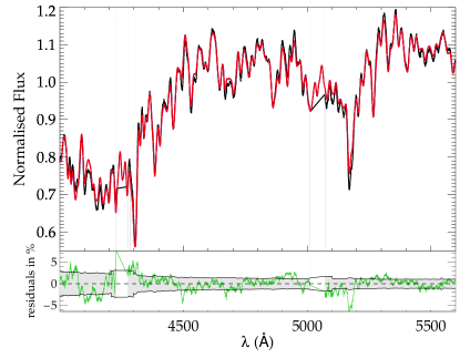
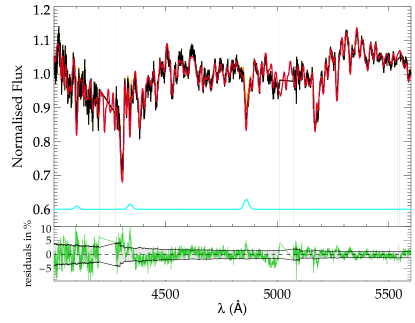
Figure 14: pPXF fit of the most central spectrum (left panel) and outermost spectrum(right panel). Black color denotes data (after emission line correction on the right panel), red color the best-fit (using the MILES SSP models with [$\alpha$/Fe]=0.0 dex and $\Gamma_{b}$=1.3), grey vertical lines masked pixels. For the right panel, the orange colored line denotes the data before emission line correction, cyan color the Balmer emission line flux that we subtracted. The lower panels show the residuals in per cent of the normalised flux in green, the grey shaded region denotes the error spectrum.

Next, we undertook fits with regularization, to obtain a smoothly weighted distribution for the template spectra. Without regularization, the optimal template may consist of several spectra with very distinct ages and metallicities, which is unphysical. Regularization produces a more realistic star formation history. It is important to find the optimal regularization parameter for each spectrum, to ensure that the weight distribution is as smooth as possible, without significantly decreasing the goodness of the fit, compared to an unregularized fit (Cappellari & Emsellem, 2004; Cappellari, 2017). We determined the optimal regularization by performing fits with a range of regularization parameters, as suggested by Cappellari (2017). We note that our regularization increases the $\chi^{2}_{\text{red}}$ value of a fit usually by less than 3 per cent, to $\chi^{2}_{red}\lesssim$1.03. The light-weighted mean age and metallicity are very similar between the unregularized fit, and the fit with optimal regularization. The best-fit age distributions of the fits have a spread of 1–2 Gyr. We repeated the fits with and without subtracting the gas emission obtained with GandALF from the Balmer line regions. The correction is only required for the outer four bins. As each SSP template model is normalised to 1 M_☉, we obtain mass-weights. We used the average flux of each SSP model in our wavelength region to transform the mass-weights to luminosity-weights.

Appendix B Stellar population models

We used three families of stellar population models, MILES models, Conroy models, and Thomas, Maraston & Johansson (TMJ) models. In this section, we briefly mention their parameter spaces and note important differences.

The MILES models are based on the code by Vazdekis et al. (2010); the newer E-MILES models (Vazdekis et al., 2016) extend over a larger wavelength range, from the ultra-violet to near-infrared. These models are only available as so-called base models, meaning that they are $\alpha$-enhanced at low metallicity, but around solar metallicity the models are scaled-solar (Vazdekis et al., 2010). There are two sets of models using different isochrones, either Padova isochrones (Girardi et al., 2000) or BaSTI (Pietrinferni et al., 2004) isochrones. Another set of models described in Vazdekis et al. (2015) is available with two different values for [$\alpha$/Fe], 0.0 and 0.4 dex, using BaSTI (Pietrinferni et al., 2004, 2006) isochrones. Depending on the isochrones, the ages and metallicities cover different ranges: 0.063–17.8 Gyr with seven metallicities from -2.32 dex to +0.22 dex for Padova isochrones, and 0.03–14 Gyr with 12 metallicities from -2.27 dex to 0.40 dex for BaSTI isochrones. However, the models with Z=0.4 dex are not considered safe (http://www.iac.es/proyecto/miles/pages/ssp-models/safe-ranges.php). Unfortunately, we do not have uncertainties for the models, which would enable us to consider also models with high metallicity at 0.4 dex.

We used the MILES models with a bimodal IMF, which is parametrized as follows: $dN/d\text{log}m\propto m^{-\Gamma}$, where the IMF slope $\Gamma$ is constant at stellar masses $M\leq$0.6 M_☉, but $\Gamma_{\text{b}}$ is varied at higher stellar masses; $\Gamma_{\text{b}}$ ranges from 0.3 (extremely bottom-light, with a dearth of low-mass stars) to 3.5 (extremely bottom-heavy, with an excess of low-mass stars) for 14 possible slope values. A bimodal IMF with $\Gamma_{\text{b}}$ = 1.3 is a good representation of a Kroupa (2001) like IMF shape. The upper and lower mass limits are at 100 M_☉ and 0.1 M_☉. We used the MILES models for spectral fitting with pPXF in Sect. 3.3.1, 4.1.2, and Appendix A.2, and for spectral indices in Sect. 4.1.1, 4.1.3, 4.2, and Appendix C. This set of models is often used for spectral index fitting in the literature.

The second family of models are from Conroy & van Dokkum (2012a), with a newer version in Conroy et al. (2018). They used the MIST isochrones (Dotter, 2016; Choi et al., 2016). The newer models cover five different ages (1, 3, 5, 9, 13.5 Gyr), five different metallicities Z (-1.5, -1.0, -0.5, 0, 0.3 dex), and variations of several elemental abundances.

The Conroy & van Dokkum (2012a) models offer only Salpeter, Chabrier, and a bottom-light IMF slope. However, the newer Conroy et al. (2018) models contain a wider range of IMF slopes, which enabled us to use them in full-spectral fitting. The IMF is defined in a different way from the MILES SSP models. In this case the high-mass IMF slope is not varied, but rather the low-mass end. Further, the slope $x$ is defined as $dN/dm\propto m^{\text{-x}}$. The IMF is parametrized as follows: The high-mass slope (1 $M_{\sun}$<m <100 $M_{\sun}$) is fixed to the Salpeter value, $x_{3}$=2.35 (not 1.35 because of the different slope definition). For lower stellar masses, the IMF is split in two IMF slopes, $x_{1}$ from 0.08–0.5 $M_{\sun}$, and $x_{2}$ from 0.5–1 $M_{\sun}$. For each IMF slope $x$, models are available for 16 slopes, ranging from 0.5 to 3.5.

To study the elemental abundances, Conroy et al. (2018) published their set of SSP models with a Kroupa (2001) IMF and with either solar abundances, or varying one of several elements (Na, Ca, Fe, C, N, Ti, Mg, Si, Ba) to a super- or sub-solar value, in most cases by $\pm$0.3 dex. Some elemental abundances are only computed with super-solar values of +0.3 dex (O+Ne+S, Sr, Cr, Mn, Eu, K, V, Cu, Ni, Co). O is varied together with the elements Ne and S, for simplicity, we will simply denote [O+Ne+S/H] as [O/H], following Johansson et al. (2012). For the Conroy & van Dokkum (2012a) models, the elements are only varied for models with an age of 13.5 Gyr and having solar metallicity, adopting a Chabrier (2003) IMF. We used the Conroy et al. (2018) models to derive corrections for spectral indices with non-solar elemental abundances in Section 4.2. Here we make the assumption that a response of the spectral index to a given elemental variation does not depend on the IMF, as we apply the same abundance correction, derived for a SSP with a Kroupa IMF, for SSPs with very different IMF slopes. We used the Conroy models in Sect. 4.2 and Appendix C for spectral index response functions, for full spectral fitting in Sect. 4.1.2 and 5, and for our simulations in Appendix D.

The third family of models are from Thomas et al. (2011b, TMJ). They cover ages from 0.1-15 Gyr, metallicities from –2.25 to 0.67 dex, [$\alpha$/Fe] = –0.3, 0.0, 0.3 and 0.5 dex. They also include several additional elemental abundances (C, N, Ca, Na, Mg, Si, Ti) enhanced to 0.3 dex. The TMJ models do not vary the IMF, and have only a fixed Salpeter (1955) IMF. We have only the published spectral index measurements and compare them to our index measurements in Sect. 4.1.1, as the TMJ models have the widest range of [$\alpha$/Fe] and Z from all model families.

Figure 15: The final NGC 3923 spectra along the major axis, normalized and shifted to rest-wavelength, from bottom to top: central 1$\farcs$5, at radii 0$\farcs$75–3″, 3″–10$\farcs$8, 10$\farcs$8–21$\farcs$6, 21$\farcs$6–43$\farcs$2, 43$\farcs$2–64$\farcs$8, 43$\farcs$2–86$\farcs$4, 64$\farcs$8–86$\farcs$4. Note that the outer three spectra overlap spatially. Several stellar absorption lines are labeled at the top of the plot.

Figure 16: The final NGC 3923 spectra at P.A. = 48° with respect to the major axis, normalized and shifted to rest-wavelength. The extraction regions were corrected such that they cover the same isophotal regions as the spectra observed along the major axis, from bottom to top: central 1$\farcs$23, at radii 0$\farcs$62–2$\farcs$46, 2$\farcs$46–8$\farcs$86, 8$\farcs$86–17$\farcs$7, 17$\farcs$7–35$\farcs$4, 35$\farcs$4–53$\farcs$1, 35$\farcs$4–70$\farcs$9, 53$\farcs$1–70$\farcs$9.

Appendix C Spectral indices

In this section we give an overview of several absorption line indices that are in common usage, and we discuss which of them are useful for our analysis.

Spectral indices are measurements of the strength of a given absorption line. A spectral index definition usually consists of a feature band definition, i.e. a wavelength region at the location of the respective absorption line, and two continuum band definitions, i.e. wavelength regions to the red and blue of the absorption line. The continuum band definition is used to estimate the pseudo-continuum in the region of the absorption line. They can be measured in units of Å or mag.

We measured spectral indices with the index definitions listed in http://www.iac.es/proyecto/miles/programs/BANDS in air wavelengths. From this list we selected indices with the following criteria: If there are several index definitions for the same absorption line, but with slightly different feature or continuum wavelength regions, we used the index definition that was designed for galaxies rather than for globular clusters. Further, we chose the spectral regions that are the least affected by emission lines and telluric absorption, and fall entirely on one rather than two IMACS chips.

We have used the MILES SSP models to investigate the indices’ sensitivity to the IMF, age, and overall metallicity; and the SSP models of Conroy & van Dokkum (2012a) to investigate the sensitivity to different elemental abundances. We now discuss the indices that are sensitive to age, metallicity, surface-gravity, and elemental abundances. Several indices are also marked on our spectra shown in Figs. 15 and 16.

Age-sensitive indices: Many absorption-line indices are sensitive to age. Together with metallicity-sensitive Fe indices, hydrogen lines can be used to derive the mean age of a stellar population (e.g. Worthey & Ottaviani, 1997; Vazdekis & Arimoto, 1999; Kuntschner et al., 2001). The hydrogen line indices for H$\alpha$, H$\beta$, H$\gamma$, H$\delta$ can decrease with stellar age. These indices are also sensitive to the metallicity, and H$\beta$ additionally to the IMF. They can also be contaminated by gas emission, which makes them sensitive to gas subtraction. We have all of these hydrogen lines in at least one of the spectra (see Figs. 15 and 16).

Metallicity-sensitive indices: The metallicity Z influences many absorption line indices. The Fe lines Fe5270, Fe5335, Fe5406 (Trager et al., 1998; McDermid et al., 2006), together with the above mentioned hydrogen lines, are often used to constrain the mean stellar metallicities of old stellar populations. These indices increase with increasing metallicity and age. Their sensitivity to most elemental abundances and the IMF is negligible compared to their sensitivity to the metallicity and [Fe/H]. There are also several Fe lines at wavelengths <3800 Å, but since our S/N is lower in this region, and the wavelength calibration less certain, we do not consider those indices. Other Fe lines, like Fe4531, Fe5709 Fe5782, are also sensitive to some elemental abundances (Ti, Mg, O), and have a mild IMF dependence.

Surface-gravity-sensitive indices: Several indices are sensitive to the surface gravity of a star, and can provide a means to discern dwarf from giant stars in old stellar populations, and thus low-mass from intermediate-mass stars. In principle, such indices can constrain the IMF slope, assuming that the effects of age, metallicity and abundances can be accounted for. Some indices increase with a higher fraction of low-mass stars, i.e. steeper IMF slope, meaning they are stronger for dwarf stars. Other indices decrease with a higher fraction of low-mass stars; they are stronger for giant stars. Among the dwarf-sensitive indices are TiO₂, bTiO, aTiO (see Fig. 17 top row), Mg₂, NaD, TiO₁, CaH₁, CaH₂, NaI₈₁₉₀, TiO_0.89, and FeH; indices that are more sensitive to giant stars and increase with decreasing IMF slope are, for example, Ca4592, Fe5709, Fe5782 (see Fig. 17 bottom row), CaHK, H$\beta_{\text{o}}$, TiO_0.85 and Ca triplet lines. (e.g. Cenarro et al., 2009; Conroy & van Dokkum, 2012a; Spiniello et al., 2014; La Barbera et al., 2016, 2017). For IMF-sensitive features in the near-infrared, further beyond the spectral range of our data, we refer the reader to Alton et al. (2017) and Lagattuta et al. (2017).

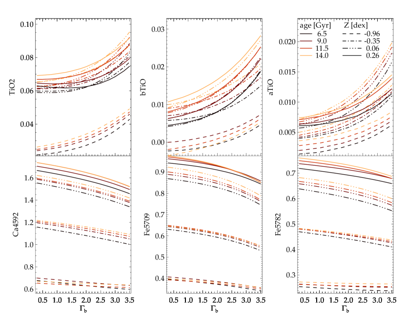
Figure 17: Dependence of different indices on the IMF slope, upper row from left to right: TiO2, bTiO, aTiO; lower row from left to right: Ca4592, Fe5709, Fe5782. Indices were measured using the MILES models with [$\alpha$/Fe]=0 dex, at FWHM=14 Å. Different colored lines denote different ages, from 6.5 Gyr (black) to 14 Gyr (orange) in steps of 2.5 Gyr, different linestyles denote different metallicities, from -0.96 (dash), -0.35 (dash-dot), +0.06 (dash-dot-dot-dot), to +0.26 dex (solid). TiO index values increase as a function of IMF slope $\Gamma_{b}$, indicating a higher sensitivity to dwarf stars (i.e. to low-mass stars in old populations). The other index values decrease as a function of $\Gamma_{b}$, indicating a higher sensitivity to giant stars (i.e. to higher-mass stars.)

We are not able to use all of these indices, for various reasons: Some indices are affected by chip gaps, e.g. Mg₂, CaH₂, TiO₁, and the Ca triplet. The NaD index at 5890 Å is also problematic, as it can be contaminated by interstellar absorption and is very sensitive to [Na/H], which has to be considered for measuring the IMF (La Barbera et al., 2017). Further, NaD and Na I are inconsistent between MILES and Conroy & van Dokkum (2012a) SSP models (Spiniello et al., 2015). For the remaining IMF-sensitive indices, we investigated their sensitivity to abundances. For example, CaHK, and CaH1 are very sensitive to [Ca/H]; Ca4592 to [Fe/H]; bTiO to [Mg/H]; H$\beta_{\text{o}}$ and aTiO to [Fe/H] and [Mg/H]; Fe5782 and TiO₂ to [O/H] and [Ti/H].

Element-abundance-sensitive indices: In order to measure the IMF slope, we have to constrain abundance variations of elements that influence IMF-sensitive indices. Based on our selection of IMF-sensitive indices and the SSP models of Conroy & van Dokkum (2012a), we have to constrain the abundances of [Mg/H], [Ti/H], [O/H], and [Fe/H].

For this reason, we searched for spectral indices that can constrain these abundances, as they are sensitive to the given element, but less so to other abundances and the IMF slope. For [Mg/H], this is best fulfilled for Mgb. For the abundances [Ti/H] and [O/H], we did not find a spectral index that is dominated by one of them. Most Ti- and O-sensitive indices are equally sensitive to other elemental abundances or the IMF slope. We did not consider spectral features with a high sensitivity to [C/H], [N/H], or [Na/H], such as CN₁, CN₂, Mg₁, or NaD. Our list of used spectral indices used is shown in Table 4.

Appendix D Simulations

To test the reliability of our spectral index fit results and to compare different sets of spectral indices and elemental abundances, we used simulations of mock spectra having the same quality as our real data (see Lonoce et al., in preparation). In particular, we investigated the level of bias and/or constraining power of the retrieved quantities when, starting from a spectrum of a certain chemical complexity, one fits only a subset of elemental abundances together with age, metallicity and IMF slopes.

For these simulations we used as input two spectra with the same chemical composition (with the exception of [C/H]), age and S/N (see Table 7), but with different IMF slopes mimicking both a bottom-heavy and a Kroupa-like IMF. Basic models with fixed age, metallicity and IMF slopes were taken from Conroy et al. (2018) models and the effect of the non-solar elemental abundances on these spectra were obtained applying the respective response functions. If certain elemental abundance values were not provided by the standard response functions, we linearly interpolated and extrapolated them. The specific choice of the elemental abundance values was similar to the results for the central radial bin of the full spectral fitting analysis (see Section 5), where we took nine abundance parameters into account in the fit.

We convolved the Conroy models to a constant velocity dispersion of $284$ km/s; this value is similar to the central radial bin of NGC 3923. We then added random noise to simulate the quality of the real data. This was done by constructing a representative S/N curve as a function of wavelength from the real data of the central radial bin and using it at each wavelength as the sigma of the random normal distribution. This S/N curve has its peak at around 6000 Å. To better delineate the biases caused by stellar parameter degeneracies, we did not include the effect of systematics in these simulations.

From the same input spectrum (input 1 or input 2), we constructed $1000$ noise realizations, and considered each of them as a single simulated object for index measurement and parameter retrieval. To retrieve the stellar parameters, we repeated the same fitting method as with real data in Sect. 4.2, calculating the $\chi^{2}$ values for all the Conroy models with the same choice of elemental abundances and sets of indices (see Table 4), putting a prior on the age (or fixing it in the multi-abundances fits) and fixing [Mg/H]=0.2. We set the steps and ranges of the parameter values as follows: 0.25 Gyr for age (ranges depending on the simulation, see Figure 18), 0.1 dex for Z (from -1.0 to 0.4 dex), 0.2 for IMF slopes $x_{1}$ and $x_{2}$ (from 0.5 to 3.5), 0.05 dex for [Ti/H] and [Fe/H] (from -0.3 to 0.3 dex), 0.05 dex for [O/H] (from 0. to 0.3 dex) and 0.05 dex for [C/H] (from -0.15 to 0.3 dex). In the case of full-spectral fitting, we used only $10$ realizations of the input spectra, and we repeated the fits as in Sec. 5.

D.1 Results of the spectral indices simulations

Figure 18: Index simulation results: each panel shows the results of simulations for a different choice of fitted parameters. All simulations were done with S/N=200 and 1000 realizations. Dashed horizontal grey lines show the true input spectral parameter values. Colors and symbols indicate different sets of indices as described in Table 4. We only show fits with a degree of freedom greater than 0. Left sets of points are the results for a Kroupa-like input IMF, right ones for a bottom-heavy input IMF. While the results for $x_{1}$ are often higher than the input values, the results for $x_{2}$ are often lower. A bottom-heavy input IMF slope is measured with higher accuracy than a Kroupa-like input IMF slope.

The results from our simulations are summarized in Figure 18 for a maximum S/N of 200 per Å. We also simulated the case with S/N=400 per Å, and found smaller statistical uncertainties, but similar biases. The $x_{1}$ slope, which characterizes the number of stars of low-mass, is poorly constrained with our available indices. Our simulations show that there is a strong bias towards high values (at the limit of the models), for both bottom-heavy and Kroupa input IMF. The least biased results are obtained when fitting both [O/H] and [C/H], but also in this case $x_{1}$ remains unconstrained with very large error bars. The choice of different index sets is irrelevant for its determination.

The $x_{2}$ slope measurements are more encouraging, as with some index sets the true values for $x_{2}$ can be retrieved. In particular, the Fe5709 (green triangles) and combined index-sets (red asterisks) results are close to the input values if the IMF is bottom-heavy. However, if it is Kroupa-like, the most accurate results for $x_{2}$ are obtained when fitting simultaneously [O/H], [C/H] and [Na/H]. It is important to choose the right combination both of indices and of elemental abundances, to avoid biases.

In general, we find that the fitted elemental abundances suffer from biases, usually independent of the choice of indices. Metallicity is very well constrained, with a small bias towards lower values in some cases. When the age is not fixed (upper panels), there are degeneracies with IMF slopes and elemental abundances, and the age is underestimated. We thus emphasize that conclusions about the IMF are dependent on assumptions about the age of the population.

D.2 Results of the full-spectral-fitting simulations

We used the same spectra as for the spectral index fitting simulations, but undertook only 10 realizations. We ran our full spectral fitting (see Sect. 5.1) routine with 5000 steps and 100 walkers, using the same wavelength regions as for the observations. In particular, we fit the short wavelength region in one case with 5 abundances (green circles in Figure 19), in another with 9 abundances (blue square symbols), the longer wavelength region including NaD with 9 abundances (orange diamonds), and including NaI and the first Ca triplet line with 9 abundances (red triangles). The exact wavelength regions of the fit and elemental abundance parameters are listed in Table 5. The mean values of the 10 realisations are shown in Figure 19 for both a Kroupa IMF and a bottom-heavy IMF.

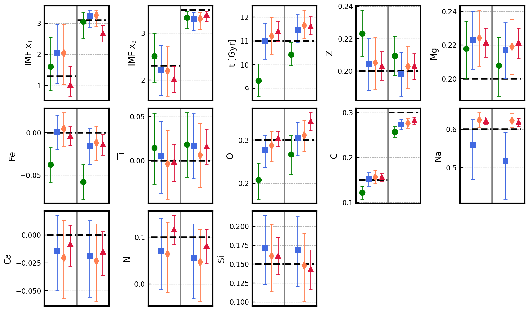
Figure 19: Full-spectral fitting simulation results: The different colors represent the results of 10 realizations of mock spectra with different wavelength regions or fitting parameters. Symbols are the same as in Figure 12 and Table 5: Green circles denote simulations of the 5-abundance fit, blue squares the 9-abundance fit, orange diamonds the 9-abundance fit when including the NaD absorption line region, and red triangles when further including the near-infrared features NaI (8200 Å) and the first CaT line (8500 Å)) regions. Including more fitting parameters and spectral features improves the accuracy and precision of our fits.

We find that the value of $x_{1}$ is poorly constrained by optical fits if the IMF is Kroupa-like. Alternatively, if the IMF is bottom-heavy, the $x_{1}$ measurement is more precise. But in both cases, $x_{1}$ tends to be overestimated. As already found for the spectral index simulations, the $x_{2}$ results are more accurate and precise. Therefore it should be possible to differentiate a very bottom-heavy value of $x_{2}$ from a more Milky-Way like value, though $x_{2}$ tends to be slightly underestimated. Including the NaI (8200 Å) and the first of the Ca Triplet lines (8500 Å), which are often used in the literature for IMF measurements, improves the precision of $x_{1}$, and $x_{2}$. For our data and simulations, these features have a lower S/N than the optical data. The measurements may be further improved by spectra of the full Ca Triplet line region at a comparable S/N as the optical data.

The stellar age is best constrained when we fit all nine abundances, but it is systematically underestimated with the 5-abundance fit, while the metallicity is slightly overestimated. These biases are less than 2 Gyr and 0.025 dex. Nevertheless, this shows that neglecting relevant elemental abundances in the fit will bias the age and metallicity results to inaccurate values.

Most element abundances are always consistent with their input values, such as [Ti/H], [Ca/H], [N/H], and [Si/H]. [Mg/H] and [Na/H] are biased to slightly higher values. This bias is only small ($\textless$0.03 dex), and may be caused by interpolation: PyStaff uses a Taylor expansion, while we used a linear interpolation to apply the response function and construct the simulated spectra. Usually, this causes differences on the sub-percent level. For high values of element abundances (e.g. [C/H] =0.3) we have to extrapolate, which can cause differences of few percent between the spectra in some spectral regions. The precision of [Na/H] improves in the fits that include the NaD absorption lines, the uncertainties decrease by a factor of four. Several uncertainties decreases even further when including the NaI and Ca Triplet features, in particular Z, [Mg/H], [Fe/H], [Ti/H], [Na/H], [Ca/H], [N/H], [Si/H] by factors of about 1.4 to 2.

We also tested fitting a slightly longer wavelength range that includes the Ca H+K line region and H$\alpha$, i.e. 3780 Å<$\lambda$<6540 Å, which are covered by our observations. We expected more precise results, and the precision for [Ca/H] and [N/H] improved by about a factor of two, but the IMF, age, and various other element abundances were unaffected. Thus, the gain in extending our wavelength region is only small, and since our data appears to have larger systematic uncertainties in the extended region, we conclude that our results will not be improved.

Overall, we find only small biases for element abundances ($\lesssim$0.05 dex). While $x_{1}$ is slightly biased to higher values, $x_{2}$ is biased to lower values in the optical fits. The simulations could recover an extremely bottom-heavy IMF, but measurements of a Kroupa IMF with optical data alone are imprecise. When including near-infrared wavelengths, $x_{1}$ and $x_{2}$ are slightly biased to lower values, but overall more precise.

Table 7: Spectral indices simulations: input spectra parameters

	Age [Gyr]	[Z/H]	$x_{1}$	$x_{2}$	[Na/H]	[Ca/H]	[Mg/H]	[Ti/H]	[Fe/H]	[C/H]	[O/H]	[N/H]	[Si/H]	S/N [Å-1]
Input 1	11.	0.2	1.3	2.3	0.6	0.0	0.2	0.0	0.0	0.15	0.3	0.1	0.2	200
Input 2	11.	0.2	3.1	3.5	0.6	0.0	0.2	0.0	0.0	0.30	0.3	0.1	0.2	200

Figure 20: PyStaff best-fit models (blue) and gas emission (red) to the central spectra (black), fitting 9 abundances. The grey color along the spectrum illustrates the noise level; vertical grey regions are excluded from the fit. The plot also shows the residuals in per cent as a function of wavelength. The upper panel (a) is the fit with Na, Ca, N, Si fixed to zero (5-abundance fit, green circles in Figures 12 and 19), the lower panel (b) is the fit with Na, Ca, N, Si as fitting parameters (9-abundance fit, blue squares in Figures 12 and 19).

Figure 21: Same as Fig. 20 for different wavelength region. The upper panel (c) is our preferred optical fit (orange diamonds in in Figs. 12 and 19). The lower panel (d) includes the near-infrared spectra (red triangles in Figs. 12 and 19).

References

- Alton et al. (2017) Alton, P. D., Smith, R. J., & Lucey, J. R. 2017, MNRAS, 468, 1594
- Alton et al. (2018) —. 2018, MNRAS, 478, 4464
- Auger et al. (2010) Auger, M. W., Treu, T., Gavazzi, R., et al. 2010, ApJ, 721, L163
- Barber et al. (2018) Barber, C., Crain, R. A., & Schaye, J. 2018, MNRAS, 479, 5448
- Bastian et al. (2010) Bastian, N., Covey, K. R., & Meyer, M. R. 2010, ARA&A, 48, 339
- Bekki (2013) Bekki, K. 2013, MNRAS, 436, 2254
- Beuing et al. (2002) Beuing, J., Bender, R., Mendes de Oliveira, C., Thomas, D., & Maraston, C. 2002, A&A, 395, 431
- Bonnell et al. (2007) Bonnell, I. A., Larson, R. B., & Zinnecker, H. 2007, in Protostars and Planets V, ed. B. Reipurth, D. Jewitt, & K. Keil, 149
- Burstein et al. (1984) Burstein, D., Faber, S. M., Gaskell, C. M., & Krumm, N. 1984, ApJ, 287, 586
- Cappellari (2017) Cappellari, M. 2017, MNRAS, 466, 798
- Cappellari & Emsellem (2004) Cappellari, M., & Emsellem, E. 2004, PASP, 116, 138
- Cappellari et al. (2012) Cappellari, M., McDermid, R. M., Alatalo, K., et al. 2012, Nature, 484, 485
- Cappellari et al. (2013) —. 2013, MNRAS, 432, 1862
- Carlsten et al. (2017) Carlsten, S. G., Hau, G. K. T., & Zenteno, A. 2017, MNRAS, 472, 2889
- Cenarro et al. (2009) Cenarro, A. J., Cardiel, N., Vazdekis, A., & Gorgas, J. 2009, MNRAS, 396, 1895
- Cenarro et al. (2003) Cenarro, A. J., Gorgas, J., Vazdekis, A., Cardiel, N., & Peletier, R. F. 2003, MNRAS, 339, L12
- Chabrier (2003) Chabrier, G. 2003, PASP, 115, 763
- Chabrier et al. (2014) Chabrier, G., Hennebelle, P., & Charlot, S. 2014, ApJ, 796, 75
- Choi et al. (2016) Choi, J., Dotter, A., Conroy, C., et al. 2016, ApJ, 823, 102
- Conroy & van Dokkum (2012a) Conroy, C., & van Dokkum, P. 2012a, ApJ, 747, 69
- Conroy & van Dokkum (2012b) Conroy, C., & van Dokkum, P. G. 2012b, ApJ, 760, 71
- Conroy et al. (2018) Conroy, C., Villaume, A., van Dokkum, P. G., & Lind, K. 2018, ApJ, 854, 139
- Da Rio et al. (2009) Da Rio, N., Gouliermis, D. A., & Henning, T. 2009, ApJ, 696, 528
- Denicoló et al. (2005) Denicoló, G., Terlevich, R., Terlevich, E., et al. 2005, MNRAS, 356, 1440
- Dotter (2016) Dotter, A. 2016, ApJS, 222, 8
- Dressler et al. (2006) Dressler, A., Hare, T., Bigelow, B. C., & Osip, D. J. 2006, in Society of Photo-Optical Instrumentation Engineers (SPIE) Conference Series, Vol. 6269, Society of Photo-Optical Instrumentation Engineers (SPIE) Conference Series, 62690F
- Ferreras et al. (2013) Ferreras, I., La Barbera, F., de La Rosa, I. G., et al. 2013, MNRAS, 429, L15
- Ferreras et al. (2008) Ferreras, I., Saha, P., & Burles, S. 2008, MNRAS, 383, 857
- Ferreras et al. (2010) Ferreras, I., Saha, P., Leier, D., Courbin, F., & Falco, E. E. 2010, MNRAS, 409, L30
- Fitzpatrick (1999) Fitzpatrick, E. L. 1999, PASP, 111, 63
- Foreman-Mackey et al. (2013) Foreman-Mackey, D., Hogg, D. W., Lang, D., & Goodman, J. 2013, PASP, 125, 306
- Garcia (1993) Garcia, A. M. 1993, A&AS, 100, 47
- Girardi et al. (2000) Girardi, L., Bressan, A., Bertelli, G., & Chiosi, C. 2000, A&AS, 141, 371
- Gregg (1994) Gregg, M. D. 1994, AJ, 108, 2164
- Ho et al. (2011) Ho, L. C., Li, Z.-Y., Barth, A. J., Seigar, M. S., & Peng, C. Y. 2011, ApJS, 197, 21
- Hopkins (2013) Hopkins, P. F. 2013, MNRAS, 433, 170
- Johansson et al. (2012) Johansson, J., Thomas, D., & Maraston, C. 2012, MNRAS, 421, 1908
- Kacharov et al. (2018) Kacharov, N., Neumayer, N., Seth, A. C., et al. 2018, MNRAS, 480, 1973
- Kausch et al. (2015) Kausch, W., Noll, S., Smette, A., et al. 2015, A&A, 576, A78
- Kroupa (2001) Kroupa, P. 2001, MNRAS, 322, 231
- Krumholz (2014) Krumholz, M. R. 2014, Phys. Rep., 539, 49
- Kuntschner (2004) Kuntschner, H. 2004, A&A, 426, 737
- Kuntschner et al. (2001) Kuntschner, H., Lucey, J. R., Smith, R. J., Hudson, M. J., & Davies, R. L. 2001, MNRAS, 323, 615
- La Barbera et al. (2013) La Barbera, F., Ferreras, I., Vazdekis, A., et al. 2013, MNRAS, 433, 3017
- La Barbera et al. (2017) La Barbera, F., Vazdekis, A., Ferreras, I., et al. 2017, MNRAS, 464, 3597
- La Barbera et al. (2016) —. 2016, MNRAS, 457, 1468
- Lagattuta et al. (2017) Lagattuta, D. J., Mould, J. R., Forbes, D. A., et al. 2017, ApJ, 846, 166
- Le Borgne et al. (2004) Le Borgne, D., Rocca-Volmerange, B., Prugniel, P., et al. 2004, A&A, 425, 881
- Leier et al. (2016) Leier, D., Ferreras, I., Saha, P., et al. 2016, MNRAS, 459, 3677
- Li et al. (2010) Li, Z.-Y., Wang, P., Abel, T., & Nakamura, F. 2010, ApJ, 720, L26
- Lyubenova et al. (2016) Lyubenova, M., Martín-Navarro, I., van de Ven, G., et al. 2016, MNRAS, 463, 3220
- Martín-Navarro et al. (2015a) Martín-Navarro, I., La Barbera, F., Vazdekis, A., Falcón-Barroso, J., & Ferreras, I. 2015a, MNRAS, 447, 1033
- Martín-Navarro et al. (2015b) Martín-Navarro, I., La Barbera, F., Vazdekis, A., et al. 2015b, MNRAS, 451, 1081
- Martín-Navarro et al. (2015c) Martín-Navarro, I., Vazdekis, A., La Barbera, F., et al. 2015c, ApJ, 806, L31
- Martín-Navarro et al. (2019) Martín-Navarro, I., Lyubenova, M., van de Ven, G., et al. 2019, A&A, 626, A124
- Massey (2003) Massey, P. 2003, ARA&A, 41, 15
- McDermid et al. (2006) McDermid, R. M., Emsellem, E., Shapiro, K. L., et al. 2006, MNRAS, 373, 906
- Mulchaey et al. (2003) Mulchaey, J. S., Davis, D. S., Mushotzky, R. F., & Burstein, D. 2003, ApJS, 145, 39
- Newman et al. (2017) Newman, A. B., Smith, R. J., Conroy, C., Villaume, A., & van Dokkum, P. 2017, ApJ, 845, 157
- Oh et al. (2011) Oh, K., Sarzi, M., Schawinski, K., & Yi, S. K. 2011, ApJS, 195, 13
- Parikh et al. (2018) Parikh, T., Thomas, D., Maraston, C., et al. 2018, MNRAS, 477, 3954
- Pietrinferni et al. (2004) Pietrinferni, A., Cassisi, S., Salaris, M., & Castelli, F. 2004, ApJ, 612, 168
- Pietrinferni et al. (2006) —. 2006, ApJ, 642, 797
- Podorvanyuk et al. (2013) Podorvanyuk, N. Y., Chilingarian, I. V., & Katkov, I. Y. 2013, MNRAS, 432, 2632
- Prieur (1988) Prieur, J. L. 1988, ApJ, 326, 596
- Sabbi et al. (2008) Sabbi, E., Sirianni, M., Nota, A., et al. 2008, AJ, 135, 173
- Salpeter (1955) Salpeter, E. E. 1955, ApJ, 121, 161
- Sansom et al. (2013) Sansom, A. E., Milone, A. d. C., Vazdekis, A., & Sánchez-Blázquez, P. 2013, MNRAS, 435, 952
- Sarzi et al. (2018) Sarzi, M., Spiniello, C., La Barbera, F., Krajnović, D., & van den Bosch, R. 2018, MNRAS, 478, 4084
- Sarzi et al. (2006) Sarzi, M., Falcón-Barroso, J., Davies, R. L., et al. 2006, MNRAS, 366, 1151
- Schlafly & Finkbeiner (2011) Schlafly, E. F., & Finkbeiner, D. P. 2011, ApJ, 737, 103
- Serra & Trager (2007) Serra, P., & Trager, S. C. 2007, MNRAS, 374, 769
- Sikkema et al. (2007) Sikkema, G., Carter, D., Peletier, R. F., et al. 2007, A&A, 467, 1011
- Smette et al. (2015) Smette, A., Sana, H., Noll, S., et al. 2015, A&A, 576, A77
- Sonnenfeld et al. (2012) Sonnenfeld, A., Treu, T., Gavazzi, R., et al. 2012, ApJ, 752, 163
- Spiniello et al. (2011) Spiniello, C., Koopmans, L. V. E., Trager, S. C., Czoske, O., & Treu, T. 2011, MNRAS, 417, 3000
- Spiniello et al. (2014) Spiniello, C., Trager, S., Koopmans, L. V. E., & Conroy, C. 2014, MNRAS, 438, 1483
- Spiniello et al. (2015) Spiniello, C., Trager, S. C., & Koopmans, L. V. E. 2015, ApJ, 803, 87
- Thomas et al. (2003) Thomas, D., Maraston, C., & Bender, R. 2003, MNRAS, 339, 897
- Thomas et al. (2005) Thomas, D., Maraston, C., Bender, R., & Mendes de Oliveira, C. 2005, ApJ, 621, 673
- Thomas et al. (2011a) Thomas, D., Maraston, C., & Johansson, J. 2011a, MNRAS, 412, 2183
- Thomas et al. (2011b) Thomas, J., Saglia, R. P., Bender, R., et al. 2011b, MNRAS, 415, 545
- Trager et al. (1998) Trager, S. C., Worthey, G., Faber, S. M., Burstein, D., & González, J. J. 1998, ApJS, 116, 1
- Treu et al. (2010) Treu, T., Auger, M. W., Koopmans, L. V. E., et al. 2010, ApJ, 709, 1195
- van Dokkum et al. (2017) van Dokkum, P., Conroy, C., Villaume, A., Brodie, J., & Romanowsky, A. J. 2017, ApJ, 841, 68
- van Dokkum (2001) van Dokkum, P. G. 2001, PASP, 113, 1420
- van Dokkum & Conroy (2010) van Dokkum, P. G., & Conroy, C. 2010, Nature, 468, 940
- van Dokkum & Conroy (2011) —. 2011, ApJ, 735, L13
- van Dokkum & Conroy (2012) —. 2012, ApJ, 760, 70
- Vaughan et al. (2018a) Vaughan, S. P., Davies, R. L., Zieleniewski, S., & Houghton, R. C. W. 2018a, MNRAS, 475, 1073
- Vaughan et al. (2018b) —. 2018b, MNRAS, 479, 2443
- Vazdekis & Arimoto (1999) Vazdekis, A., & Arimoto, N. 1999, ApJ, 525, 144
- Vazdekis et al. (2016) Vazdekis, A., Koleva, M., Ricciardelli, E., Röck, B., & Falcón-Barroso, J. 2016, MNRAS, 463, 3409
- Vazdekis et al. (2010) Vazdekis, A., Sánchez-Blázquez, P., Falcón-Barroso, J., et al. 2010, MNRAS, 404, 1639
- Vazdekis et al. (2015) Vazdekis, A., Coelho, P., Cassisi, S., et al. 2015, MNRAS, 449, 1177
- Weijmans et al. (2009) Weijmans, A.-M., Cappellari, M., Bacon, R., et al. 2009, MNRAS, 398, 561
- Worthey et al. (1994) Worthey, G., Faber, S. M., Gonzalez, J. J., & Burstein, D. 1994, ApJS, 94, 687
- Worthey & Ottaviani (1997) Worthey, G., & Ottaviani, D. L. 1997, ApJS, 111, 377