Replica evolution of classical field in 4+1 dimensional spacetime toward real time dynamics of quantum field 

Abstract

Real-time evolution of replicas of classical field is proposed as an approximate simulator of real-time quantum field dynamics at finite temperatures. We consider $N$ classical field configurations, $(\phi_{{\tau{\bm{x}}}},\pi_{{\tau{\bm{x}}}})(\tau=0,1,\cdots N-1)$, dubbed as replicas, which interact with each other via the $\tau$-derivative terms and evolve with the classical equation of motion. The partition function of replicas is found to be proportional to that of quantum field in the imaginary time formalism. Since the replica index can be regarded as the imaginary time index, the replica evolution is technically the same as the molecular dynamics part of the hybrid Monte-Carlo sampling. Then the replica configurations should reproduce the correct quantum equilibrium distribution after the long-time evolution. At the same time, evolution of the replica-index average of field variables is described by the classical equation of motion when the fluctuations are small. In order to examine the real-time propagation properties of replicas, we first discuss replica evolution in quantum mechanics. Statistical averages of observables are precisely obtained by the initial condition average of replica evolution, and the time evolution of the unequal-time correlation function, $\langle x(t)x(t^{\prime})\rangle$, in a harmonic oscillator is also described well by the replica evolution in the range $T/\omega>0.5$. Next, we examine the statistical and dynamical properties of the $\phi^{4}$ theory in the 4+1 dimensional spacetime, which contains three spatial, one replica index or the imaginary time, and one real time. We note that the Rayleigh-Jeans divergence can be removed in replica evolution with $N\geq 2$ when the mass counterterm is taken into account. We also find that the thermal mass obtained from the unequal-time correlation function at zero momentum grows as a function of the coupling as in the perturbative estimate in the small coupling region.

1 Introduction

Classical dynamics has been utilized to understand non-equilibrium evolution of quantum many-body systems in various fields of physics TDGP ; TDHF ; inflation ; CSS ; CYM ; Dumitru-Nara ; YM-chaos ; Entropy ; Shear ; Matsuda . The classical equation of motion for the phase space distribution (Vlasov equation) Vlasov is known to provide an approximate solution of the quantum equation of motion for the density matrix (von Neumann equation) vonNeumann , provided that the classical analogue of the quantum mechanical distribution function Wigner is given as the initial condition and the $\mathcal{O}(\hbar^{2})$ effects are negligible. It is also known that one can numerically obtain the solution of the Vlasov equation by solving the classical equations of motion for particle ensemble representing the phase space distribution TP . This favorable feature of classical dynamics has been invoked also in field theories inflation ; CSS ; CYM ; Dumitru-Nara ; YM-chaos ; Entropy ; Shear ; Matsuda . For example, the classical Yang-Mills (CYM) field has been adopted to describe the initial stage of high-energy heavy-ion collisions, and have provided important insights into the non-equilibrium dynamics of the gluon field CYM ; Dumitru-Nara ; YM-chaos ; Entropy ; Matsuda .

Compared with the successes in the far-from-equilibrium stages, the applicability of classical dynamics is limited when discussing equilibrium properties of quantum systems. Since the equipartition law applies to classical equilibrium, the number of high-momentum particles is overestimated and one encounters the Rayleigh-Jeans divergence. One possible way to manage the divergence is treating the hard modes above the cutoff separately. By integrating hard modes Bodeker:1995pp ; Greiner:1996dx or by introducing the mass counterterm Aarts , one can obtain the effective action of the classical field, soft modes below the cutoff, and utilize the action to evaluate the evolution. In CYM theory, dynamical evolution of the coupled system of classical field and particles is explicitly solved and was demonstrated to promote equilibration Dumitru-Nara . Still, classical field obeys classical statistics, then the cutoff momentum should be chosen to be of the order of $T$ or smaller also in these frameworks. While the two-particle irreducible (2PI) effective action approach can treat classical field and particles on the same footing Berges:2004yj ; Aarts:2001yn ; Hatta-Nishiyama , the numerical cost is large and it is not yet easy to apply to realistic systems under inhomogeneous classical field.

Thus it is desirable to develop frameworks which inherit the merit of classical field dynamics but properly describe quantum statistical equilibrium after a long-time evolution. Including these two features is known to be important in nuclear transport phenomena QStat , and it is desirable also to describe non-equilibrium phenomena in field theories as mentioned above. In the stochastic quantization SQ , one can obtain field configurations $\{\phi\}$ by solving the Langevin equation, $d\phi_{x}/dt=-\partial S/\partial\phi_{x}+\zeta_{x}$, with $t$ being the fictitious time and $\zeta_{x}$ being the white noise, $\left\langle{\zeta_{x}(t)\zeta_{y}(t^{\prime})}\right\rangle=2\delta_{xy}\delta(t-t^{\prime})$. The field distribution approaches the quantum one, while the above Langevin equation cannot be regarded as the equation of motion to describe the real time evolution. There is a hint to incorporate the quantum statistical property into the real time evolution in the imaginary time formalism of finite temperature quantum field theory, where the field variables in 3D space are enlarged to those in 3+1D spacetime introducing the imaginary time. In the path integral representation, the thermally equilibrated quantum field distribution is described by $\exp(-S[\phi])$, where $S[\phi]$ is the 3+1D Euclidean action. In the molecular dynamics part of the hybrid Monte-Carlo (HMC) sampling HMC , the Hamiltonian is set to be $\mathcal{H}=\sum\pi_{\bm{x}\tau}^{2}/2+S[\phi]$ with $\pi_{\bm{x}\tau}$ being the canonical conjugate of the field variable $\phi_{\bm{x}\tau}$ at a spacetime point $(\bm{x},\tau)$, where $\tau$ is the imaginary time coordinate. The classical equation of motion, $d\phi_{\bm{x}\tau}/dt=\partial\mathcal{H}/\partial\pi_{\bm{x}\tau}$ and $d\pi_{\bm{x}\tau}/dt=-\partial\mathcal{H}/\partial\phi_{\bm{x}\tau}$, is solved with the initial condition of $\left\langle{\pi_{\bm{x}\tau}^{2}}\right\rangle=1$, where the time variable $t$ is the fictitious simulation time and introduced in an ad hoc manner. After a long-time evolution, the system reaches the equilibrium described by the classical partition function at temperature of unity, $\mathcal{Z}=\int\mathcal{D}\pi\,\mathcal{D}\phi\,\exp(-\mathcal{H})\propto\int\mathcal{D}\phi\,\exp(-S[\phi])$, then we can correctly sample the quantum field configuration in equilibrium.

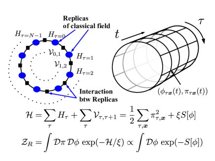
Figure 1: Replicas and their evolution. Replica configuration $(\phi_{\tau\bm{x}},\pi_{\tau\bm{x}})$ evolves with the classical equation of motion using the Hamiltonian $\mathcal{H}$. The interaction part of the replica Hamiltonian $\mathcal{H}$ is chosen so that the $\phi$ part of $\mathcal{H}$ agrees with the Euclidean action $S[\phi]$ multiplied by the lattice anisotropy $\xi=a/a_{\tau}$. Thus the replica partition function $\mathcal{Z}$ becomes proportional to the equilibrium quantum field partition function, $\int\mathcal{D}\exp(-S[\phi])$.

In this article, we examine the time evolution of the enlarged field variables in the 3+1 dimensions, $(\phi_{\bm{x}\tau},\pi_{\bm{x}\tau})$, a set of 3D classical field configurations referred to as replicas, and propose that this can be regarded as the real time evolution of 3D quantum field in equilibrium. Each replica with the index $\tau$ corresponds to the field configuration on each (discretized) imaginary time coordinate in the finite temperature quantum field theory, and then the replica evolution is practically equivalent to the molecular dynamics part of HMC. As schematically shown in Fig. 1, the replica Hamiltonian $\mathcal{H}$ is given as the sum of the Hamiltonian of each replica plus the interactions between the nearest neighbor replicas, $\mathcal{V}_{\tau,\tau+1}$, which is referred to as the $\tau$-derivative term and causes thermalization of replicas. The distribution of one replica configuration regarded as the system relaxes to the quantum equilibrium distribution by the $\tau$-derivative interactions with other replicas regarded as the heat bath. Thus, on the one hand, field variables $\phi$ reaches correct quantum statistical distribution after a long-time replica evolution. On the other hand, the replica-index average of field variables obeys the standard classical field equation of motion when fluctuations are small as shown later, and then the variable $t$, the fictitious simulation time in HMC, works as the real time variable in the replica evolution. Hence the replica evolution can reproduce both the quantum statistics and the classical evolution in these two limits. These features of the replica evolution are encouraging for us to consider it as a candidate which describes dynamical evolution of quantum field, while the formal justification of the replica evolution as a quantum time evolution has not been found. In order to examine the validity of replica evolution, we investigate the real-time evolution of the unequal-time two-point function at zero momentum numerically without and with the mass counterterm. We demonstrate that the thermal mass obtained from the replica evolution is consistent with the perturbative calculation results in quantum field theory. While the longer term goal is to apply the replica evolution to the non-equilibrium real time evolution of a system of fields, we here concentrate on the equilibrium features as the first step toward the goal.

This article is organized as follows. In Sec. 2.2, we introduce the replica evolution in quantum mechanics, and the statistical and dynamical properties of a harmonic oscillator are examined. In Sec. 3, we introduce the replica evolution in classical field, and the statistical properties of replicas are examined in the free field case. We also discuss the mass counterterm on the lattice. In Sec. 4, we show the results of real-time evolution of replicas in the $\phi^{4}$ theory. By using the damped oscillator ansatz, we fit the unequal-time two-point function of replica evolution, and compare the obtained thermal mass and damping rate with the perturbative calculation results. Section 5 is devoted to the summary and perspectives.

2 Replica evolution in quantum mechanics

In this section, we introduce the replica evolution in quantum mechanics. We consider $N$ sets of canonical variables, which are labeled by the replica index $\tau$ and are the functions of time $t$, $(\bm{x}_{\tau}(t),\bm{p}_{\tau}(t))$. As shown in Fig. 1, there are two variables, $\tau$ and $t$, which are related to time: The variable $\tau$ is proportional to the continuous temporal variable $\bar{\tau}$, $\tau/\xi\to\bar{\tau}$, in the large $N$ limit in the imaginary time formalism, and we regard it as an index of the replica. The time $t$ corresponds to the fictitious simulation time in HMC, and is found to work as the real time in the replica evolution.

2.1 Statistics and dynamics of replicas in quantum mechanics

In this section, we introduce replica evolution in quantum mechanics and examine its statistical and dynamical properties. We consider the classical system described by the following Hamiltonian

$$H(\bm{x},\bm{p})= \frac{\bm{p}^{2}}{2}+V(\bm{x})=\sum_{i=1}^{D}\frac{p_{i}^{2}}{2}+V(\bm{x}),$$ (1)

where the mass is set to be unity for simplicity, and $D$ is the number of components in $\bm{x}$ and $\bm{p}$. We now consider $N$ replicas of canonical variables, $(\bm{x}_{\tau},\bm{p}_{\tau})(\tau=0,1,\cdots,N\!-\!1)$, whose Hamiltonian is given by the sum of the Hamiltonians $H(\bm{x}_{\tau},\bm{p}_{\tau})$ over the replica indices $\tau$ and the $\tau$-derivative terms,

$$\mathcal{H}= \sum_{\tau}H(\bm{x}_{\tau},\bm{p}_{\tau})+\mathcal{V}\ ,\quad\mathcal{V}=\frac{\xi^{2}}{2}\sum_{\tau}(\bm{x}_{\tau+1}-\bm{x}_{\tau})^{2}\ .$$ (2)

The periodic boundary condition is imposed in the $\tau$ direction, $(\bm{x}_{N},\bm{p}_{N})=(\bm{x}_{0},\bm{p}_{0})$. The replicas are assumed to evolve in real time $t$ according to the canonical equations of motion,

$$\frac{d\bm{x}_{\tau}}{dt}= \frac{\partial\mathcal{H}}{\partial\bm{p}_{\tau}}\ ,\quad\frac{d\bm{p}_{\tau}}{dt}=-\frac{\partial\mathcal{H}}{\partial\bm{x}_{\tau}}\ .$$ (3)

The replica evolution with Eq. (3) has two distinct features: First, the ensemble of replica configurations follows the quantum statistical distribution of the spatial variables $x=\{\bm{x}_{\tau}|\tau=0,1,\cdots,N-1\}$ in the long-time evolution. Second, the evolution of replica-index average agrees with the purely classical evolution, when the fluctuations among replicas are small.

Let us examine the first point on the statistics of replicas. The partition function of replicas at temperature $T_{\mathrm{repl}}=\xi$ is given as

$$\mathcal{Z}_{R}(\xi)= \int\prod_{\tau}\frac{d\bm{x}_{\tau}d\bm{p}_{\tau}}{(2\pi)^{D}}e^{-\mathcal{H}/\xi}=\frac{\xi^{ND/2}}{(2\pi)^{ND}}\int\prod_{\tau}d\bm{x}_{\tau}e^{-S(x)}\ ,$$ (4)

$$S(x)= \frac{1}{\xi}\sum_{\tau}\left[\frac{\xi^{2}}{2}\left(\bm{x}_{\tau+1}-\bm{x}_{\tau}\right)^{2}+V(\bm{x}_{\tau})\right]\underset{N\to\infty}{\longrightarrow}S_{E}[x]=\int_{0}^{\beta}d\bar{\tau}L_{E}\left(x,\frac{\partial x}{\partial\bar{\tau}}\right)\ ,$$ (5)

$$L_{E}= \frac{1}{2}\left[\frac{\partial\bm{x}(\bar{\tau})}{\partial\bar{\tau}}\right]^{2}+V(\bm{x}(\bar{\tau}))$$ (6)

where $\beta=N/\xi$ and $\tau/\xi\to\bar{\tau}$ is the continuous imaginary time. Since $S_{E}[x]$ is the Euclidean action at temperature $T=1/\beta=\xi/N$ in the imaginary time formalism, the replica partition function $\mathcal{Z}_{R}$ at temperature $T_{\mathrm{repl}}=\xi$ is proportional to the quantum mechanical partition function at $T=\xi/N$ in the large $N$ limit. Thus observables as functions of $x$ in quantum equilibrium are correctly obtained from the thermal average of observables $\left\langle{\mathcal{O}(\bm{x})}\right\rangle_{T}$ in classical equilibrium of replica configurations,

$$\left\langle{\mathcal{O}(\bm{x})}\right\rangle_{T}\equiv \left\langle{\mathcal{O}(\bm{x_{\tau^{\prime}}})}\right\rangle=\frac{1}{\mathcal{Z}_{R}(\xi)}\int\prod_{\tau}\frac{d\bm{x}_{\tau}d\bm{p}_{\tau}}{(2\pi)^{D}}\,e^{-\mathcal{H}/\xi}\,\mathcal{O}(\bm{x}_{\tau^{\prime}})$$

$$= \int\prod_{\tau}{d\bm{x}_{\tau}}\,e^{-S(x)}\,\widetilde{\mathcal{O}}(\bm{x})\,/\,\int\prod_{\tau}{d\bm{x}_{\tau}}\,e^{-S(x)},$$ (7)

where $\tau^{\prime}$ in the first line is the replica index of observation, and in the second line, we replace $\mathcal{O}(\bm{x}_{\tau^{\prime}})$ with the “replica-index average”,

$$\widetilde{\mathcal{O}}(\bm{x},\bm{p})=\frac{1}{N}\sum_{\tau}\mathcal{O}(\bm{x}_{\tau},\bm{p}_{\tau}),$$ (8)

using the translational invariance in the $\tau$-direction. Then, a thermal expectation value of an operator $\left\langle{O(\bm{x})}\right\rangle_{T}$ can be obtained as an expectation value of the replica-index averaged operator,

$$\left\langle{\mathcal{O}(\bm{x})}\right\rangle_{T}=\left\langle{\widetilde{\mathcal{O}}(\bm{x})}\right\rangle.$$ (9)

In the imaginary time formalism, the thermal average of an observable in quantum mechanics is given as

$$\left\langle{\mathcal{O}(\bm{x})}\right\rangle= \mathrm{tr}(\mathcal{O}(\bm{x})\,e^{-\beta H})/\mathrm{tr}(e^{-\beta H})=\int\mathcal{D}xe^{-S_{E}[x]}\,\mathcal{O}(\bm{x}(\bar{\tau}^{\prime}))/\int\mathcal{D}xe^{-S_{E}[x]},$$ (10)

where the imaginary time of observation $\bar{\tau}^{\prime}$ appears in the path integral representation. After replacing $\mathcal{O}(\bm{x}(\bar{\tau}^{\prime}))$ with its imaginary time average, the quantum statistical average (10) is found to be described by the replica average (7) in the large $N$ limit.

The classical equilibrium of replica configurations can be generally obtained by the long-time evolution with the canonical equation of motion, Eq. (3), due to the chaoticity of the system. Practically, it is useful to take the “replica ensemble average” instead of the long-time average, since there is no autocorrelation in the former. We prepare $N_{\mathrm{conf}}(\gg 1)$ initial replica configurations $\left\{(x^{(i)},p^{(i)})|i=1,2,\cdots,N_{\mathrm{conf}}\right\}$ at $t=0$ appropriately, solve the equation of motion, then the replica average is calculated as

$$\left\langle{\mathcal{O}(\bm{x})}\right\rangle\simeq \lim_{t\to\infty}\frac{1}{N_{\mathrm{conf}}}\sum_{i=1}^{N_{\mathrm{conf}}}\widetilde{\mathcal{O}}(x^{(i)}(t))=\lim_{t\to\infty}\frac{1}{N_{\mathrm{conf}}}\sum_{i=1}^{N_{\mathrm{conf}}}\frac{1}{N}\sum_{\tau=0}^{N-1}\mathcal{O}(\bm{x}_{\tau}^{(i)}(t)).$$ (11)

Let us turn to the second point. While replica ensemble simulates quantum statistical ensemble after a long-time evolution, the replica-index averages of the canonical variables evolve as the classical variables when the fluctuations among replicas are small. The equation of motion for the replica-index average of the canonical variables reads

$$\frac{d\widetilde{\bm{x}}}{dt}= \frac{1}{N}\sum_{\tau}\frac{d\bm{x}_{\tau}}{dt}=\frac{1}{N}\sum_{\tau}\bm{p}_{\tau}=\widetilde{\bm{p}},$$ (12)

$$\frac{d\widetilde{\bm{p}}}{dt}= \frac{1}{N}\sum_{\tau}\frac{d\bm{p}_{\tau}}{dt}=-\frac{1}{N}\sum_{\tau}\frac{\partial\mathcal{H}}{\partial\bm{x}_{\tau}}=-\frac{1}{N}\sum_{\tau}\frac{\partial V(\bm{x}_{\tau})}{\partial\bm{x}_{\tau}}$$

$$= -\frac{\partial V(\widetilde{\bm{x}})}{\partial\widetilde{\bm{x}}}-\frac{1}{2}\sum_{i,j}\frac{\partial^{3}V(\widetilde{\bm{x}})}{\partial\widetilde{\bm{x}}\partial\widetilde{x}_{i}\partial\widetilde{x}_{j}}\frac{1}{N}\sum_{\tau}(x_{i\tau}-\widetilde{x}_{i})(x_{j\tau}-\widetilde{x}_{j})+\mathcal{O}((\delta x)^{3})$$

$$= -\frac{\partial V(\widetilde{\bm{x}})}{\partial\widetilde{\bm{x}}}+\mathcal{O}((\delta x)^{2}),$$ (13)

where $x_{i\tau}$ is the $i$-th component of $\bm{x}_{\tau}$ and $(\delta x)^{2}=\sum_{\tau}(\bm{x}_{\tau}-\widetilde{\bm{x}})^{2}/N$ is the fluctuations of $\bm{x}_{\tau}$ in one configuration of replicas. It should be noted that the $\tau$-derivative terms do not operate because of the periodic boundary condition, and the second derivative terms of $V$ disappear from the definition of $\widetilde{\bm{x}}$. It is interesting to find that the first line of Eq. (13) shows the Ehrenfest’s theorem

$$\frac{d^{2}\left\langle{x}\right\rangle}{dt^{2}}=-\left\langle{\frac{\partial V(x)}{\partial x}}\right\rangle,$$ (14)

where $\left\langle{\cdots}\right\rangle$ denotes the replica-index average here. Then when $(\delta x)^{2}$ is small, these equations of motion tell us the classical nature of the replica-index average,

$$\frac{d^{2}\widetilde{\bm{x}}}{dt^{2}}\simeq -\frac{\partial V(\widetilde{\bm{x}})}{\partial\widetilde{\bm{x}}}.$$ (15)

By comparison, $(\delta x)^{2}$ should be a part of quantum fluctuations.

2.2 Replica evolution of harmonic oscillator

We now look further into the dynamical property of replicas of a single harmonic oscillator. By choosing $V=\omega^{2}x^{2}/2$ and $D=1$ in Eq. (1), the Hamiltonian is given as

$$H(x,p)= \frac{1}{2}p^{2}+\frac{\omega^{2}}{2}x^{2}=\omega\left(a^{\dagger}a+\frac{1}{2}\right),\quad a=\frac{1}{\sqrt{2}}\left(\sqrt{\omega}x+\frac{ip}{\sqrt{\omega}}\right).$$ (16)

In order to investigate the statistical properties of replicas, it is useful to adopt the Fourier transform with respect to the replica index,

$$\bar{x}_{n}=\frac{1}{\sqrt{N}}\sum_{\tau}e^{i\omega_{n}\tau}x_{\tau}\ ,\quad\bar{p}_{n}=\frac{1}{\sqrt{N}}\sum_{\tau}e^{i\omega_{n}\tau}p_{\tau}\ ,$$ (17)

where $\omega_{n}=2\pi n/N$ denotes the Matsubara frequency. With $(\bar{x}_{n},\bar{p}_{n})$, the Hamiltonian is represented by that of the $N$ free harmonic oscillators,

$$\mathcal{H}= \sum_{n}\left[\frac{1}{2}\bar{p}_{n}^{2}+\frac{M_{n}^{2}}{2}\bar{x}_{n}^{2}\right]\ ,\quad M_{n}^{2}=\,\omega^{2}+4\xi^{2}\sin^{2}(\omega_{n}/2)\ .$$ (18)

The replica partition function is obtained as

$$\mathcal{Z}_{R}(\xi)= \prod_{n}\left(\int\frac{d\bar{x}_{n}d\bar{p}_{n}}{2\pi}e^{-\bar{p}_{n}^{2}/2\xi-M_{n}^{2}\bar{x}_{n}^{2}/2\xi}\right)=\prod_{n}\left(\frac{\xi}{M_{n}}\right)\ .$$ (19)

By using the Matsubara frequency summation formula explained in Appendix A, the logarithm of the partition function is found to be

$$-\log\mathcal{Z}_{R}(\xi)= \sum_{n}\log(M_{n}/\xi)=\frac{1}{2}\sum_{n}\log\left[\left(\frac{\omega}{2\xi}\right)^{2}+\sin^{2}(\omega_{n}/2)\right]+N\log 2$$

$$= \log\left[2\sinh\left(\frac{\Omega}{2T}\right)\right]\underset{N\to\infty}{\longrightarrow}\log\left[2\sinh\left(\frac{\omega}{2T}\right)\right]\ ,$$ (20)

where $\Omega$ is given as

$$\Omega =2\xi\,\mathrm{arcsinh}\,(\omega/2\xi)=2NT\,\mathrm{arcsinh}\,(\omega/2NT)\underset{N\to\infty}{\longrightarrow}\omega\ .$$ (21)

The replica partition function, Eq. (19), at large $N$ agrees with the quantum mechanical partition function at $T=\xi/N$,

$$\mathcal{Z}_{Q}(T)= \sum_{n=0}^{\infty}e^{-E_{n}/T}=\sum_{n=0}^{\infty}e^{-\omega/T(n+1/2)}=\frac{e^{-\omega/2T}}{1-e^{-\omega/T}}=\left[2\sinh\left(\frac{\omega}{2T}\right)\right]^{-1}\ .$$ (22)

Thus we find that it is possible to obtain quantum statistical results by using a replica ensemble in equilibrium, a large number of configurations of $N$ sets of canonical variables, $(x_{\tau},p_{\tau})$, which are prepared to be in classical equilibrium.

We next examine the time-evolution of replicas by using the time-correlation function, $C(t)=\left\langle{x(t)x(0)}\right\rangle$. For preparation, let us recall the quantum mechanical results. The time correlation of the spatial coordinate is calculated as

$$\left\langle{\,\psi|x_{H}(t)x_{H}(0)|\psi\,}\right\rangle=\left\langle{\,\psi|e^{iHt}xe^{-iHt}x|\psi\,}\right\rangle$$

$$= \frac{1}{2\omega}\sum_{n,n^{\prime}}c_{n}^{*}c_{n^{\prime}}\left\langle{n|e^{iHt}(a+a^{\dagger})e^{-iHt}(a+a^{\dagger})|n^{\prime}}\right\rangle$$

$$= \frac{1}{2\omega}\sum_{n}\left\{c_{n}^{*}c_{n}\left[ne^{i\omega t}+(n+1)e^{-i\omega t}\right]+\sqrt{n(n-1)}\left[c_{n-2}^{*}c_{n}e^{-i\omega t}+c_{n}^{*}c_{n-2}e^{i\omega t}\right]\right\}\ ,$$ (23)

where $x_{H}$ is the operator in the Heisenberg picture, $|n\rangle$ is the energy eigen state, $c_{n}$ is the expansion coefficient, $|\psi\rangle=\sum_{n}c_{n}|n\rangle$, and we have used the relations, $\left\langle{n\!-\!1|a|n}\right\rangle=\sqrt{n}$ and $\left\langle{n\!+\!1|a^{\dagger}|n}\right\rangle=\sqrt{n\!+\!1}$. In thermal equilibrium at temperature $T$, the density matrix becomes diagonal and the statistical weights are given by the Boltzmann factor,

$$\rho_{nn^{\prime}}=\left\langle{c_{n}c_{n^{\prime}}^{*}}\right\rangle_{T}=\frac{e^{-\omega(n+1/2)/T}}{\mathcal{Z}_{Q}}\delta_{nn^{\prime}}\ .$$ (24)

Thus the time-correlation function in thermal equilibrium is obtained as

$$C_{Q}(t)= \left\langle{x_{H}(t)x_{H}(0)}\right\rangle_{T}=\frac{1}{2\omega}\sum_{n}\frac{e^{-n\omega/T}}{\mathcal{Z}_{Q}}\left[ne^{i\omega t}+(n+1)e^{-i\omega t}\right]$$

$$= \frac{1}{2\omega}\left[\coth\left(\frac{\omega}{2T}\right)\cos\omega t-i\sin\omega t\right]\ ,$$ (25)

where we have used the relation $\sum_{n}ne^{-nx}=d/dx(\sum_{n}e^{-nx})$ to obtain the second line. Since the expectation value of symmetrized product (Weyl ordering) is obtained in classical dynamics, we are interested in the time-even part part of the time-correlation function given as

$$C_{Q}^{\mathrm{even}}(t)= \left\langle{\frac{1}{2}\,\left\{x_{H}(t),x_{H}(0)\right\}}\right\rangle_{T}=\frac{\coth(\omega/2T)}{2\omega}\,\cos\omega t\to\frac{T}{\omega^{2}}\,\cos\omega t\ (T/\omega\gg 1)\ .$$ (26)

In replica evolution, it is easier to solve the canonical equation of motion in the Fourier transform. The equations of motion are, $d\bar{x}_{n}/dt=\partial\mathcal{H}/\partial\bar{p}_{n}=\bar{p}_{n}$ and $d\bar{p}_{n}/dt=-\partial\mathcal{H}/\partial\bar{x}_{n}=-M_{n}^{2}\bar{x}_{n}$, and the solution is obtained as

$$\bar{x}_{n}(t)=\bar{x}_{n}(0)\cos M_{n}t+\frac{\bar{p}_{n}(0)}{M_{n}}\sin M_{n}t\ ,\quad\frac{\bar{p}_{n}(t)}{M_{n}}=-\bar{x}_{n}(0)\sin M_{n}t+\frac{\bar{p}_{n}(0)}{M_{n}}\cos M_{n}t\ .$$ (27)

We evaluate thermal average imposing thermal distribution to the initial field variables, $\bar{x}_{n}(0)$ and $\bar{p}_{n}(0)$. Since the Boltzmann weight is given as $\exp(-\mathcal{H}/\xi)=\exp[-\sum_{n}(\bar{p}_{n}^{2}/2\xi+\bar{x}_{n}^{2}/2M_{n}^{2}\xi)]$, the distributions of $\bar{x}_{n}$ and $\bar{p}_{n}$ in equilibrium are gaussians, $\left\langle{\bar{x}_{n}(0)\bar{x}_{n^{\prime}}(0)}\right\rangle_{T}=\xi/M_{n}^{2}\delta_{nn^{\prime}}$ and $\left\langle{\bar{p}_{n}(0)\bar{p}_{n^{\prime}}(0)}\right\rangle_{T}=\xi\delta_{nn^{\prime}}$. Then the time-correlation function is obtained as

$$C_{R}(t)= \left\langle{x(t)x(0)}\right\rangle_{T}\equiv\frac{1}{N}\sum_{\tau}\left\langle{x_{\tau}(t)x_{\tau}(0)}\right\rangle_{T}=\frac{1}{N}\sum_{n}\left\langle{\bar{x}_{n}(t)\bar{x}_{n}(0)}\right\rangle_{T}=\frac{1}{N}\sum_{n}\frac{\xi}{M_{n}^{2}}\,\cos M_{n}t$$

$$= \sum_{n}\frac{T}{M_{n}^{2}}\,\cos M_{n}t\ .$$ (28)

We here adopt the replica-index average, the average of the time-correlation function over the replica indices $\tau$, and the replica ensemble average, the average over the initial configurations. The zero Matsubara frequency contribution in the replica formalism agrees with the quantum mechanical result in the high-temperature limit,

$$C_{R0}(t)=\frac{1}{N}\left\langle{\bar{x}_{0}(t)\bar{x}_{0}(0)}\right\rangle=\left\langle{\tilde{x}(t)\tilde{x}(0)}\right\rangle=\frac{T}{\omega^{2}}\,\cos\omega t\ ,$$ (29)

where $\tilde{x}=\sum_{\tau}x_{\tau}/N$ is the replica-index average of $x_{\tau}$. The other Matsubara frequencies lead to higher harmonics, which do not appear in the quantum mechanical result. Yet they play an essential role to explain the value of equal-time correlation $C_{R}(0)=\left\langle{x^{2}(0)}\right\rangle$ at lower temperatures,

$$C_{R}(0)= \sum_{n}\frac{T}{M_{n}^{2}}=\sum_{n}\frac{T}{\omega^{2}+4\xi^{2}\sin^{2}(\omega_{n}/2)}=\frac{1}{2\omega}\frac{\coth(\Omega/2T)}{\sqrt{1+(\omega/2\xi)^{2}}}\underset{N\to\infty}{\longrightarrow}\frac{\coth(\omega/2T)}{2\omega}\ .$$ (30)

In Fig. 2, we show the temperature dependence of the equal-time correlation function, $C(0)=\left\langle{x^{2}}\right\rangle$, which provides the amplitude of $C(t)$. As already mentioned, $C_{R0}(0)$ agrees with the quantum mechanical result at high temperatures, $T\gtrsim\omega$. At lower temperatures, $C_{R0}(0)$ itself deviates from the quantum mechanical result, while the other Matsubara frequency contribution lifts up the amplitude. As a result, the amplitude in the replica method increases with increasing $N$, and converges to quantum mechanical result in the large $N$ limit. We confirm that the replica method reproduces the quantum mechanical result of the equal-time correlation $\left\langle{x^{2}}\right\rangle=C_{Q}(0)$ in the large $N$ limit, which is not a total surprise since the replica method gives correct thermal quantum distribution after a long-time evolution.

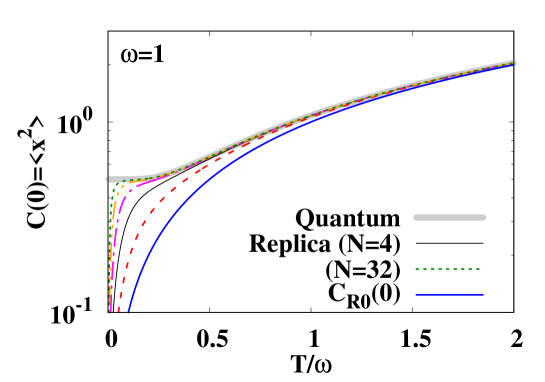
Figure 2: Equal-time correlation function of a harmonic oscillator. Grey solid curve shows the quantum mechanical results ($C_{Q}$), the blue solid curve shows the classical field results ($C_{R0}$), and other curves show the replica evolution results ($C_{R}$, $N>1$); red dashed, black solid, magenta dot-dashed, orange dot-dot-dashed, and green dotted curves show the results with $N=2,4,8,16$ and 32, respectively.

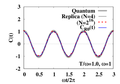
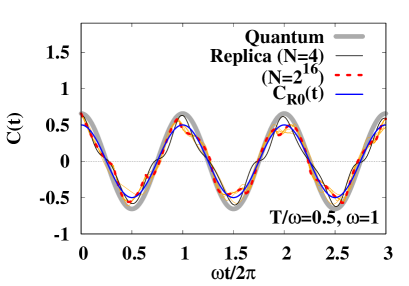
Figure 3: Time-correlation function of a harmonic oscillator. Grey solid curve shows the quantum mechanical results ($C_{Q}(t)$), the blue solid curve shows the classical field results ($C_{R0}(t)$), and other curves show the replica evolution results ($C_{R}(t)$, $N>1$); black solid and red dotted curves show the results with $N=4$ and $N=2^{16}$, respectively, and orange curves show other results with $N=2^{1-15}$.

Let us come back to the evaluation of the time-correlation functions. In Fig. 3, we show the time-correlation function of a harmonic oscillator in quantum mechanics and in the replica evolution. When the temperature $T$ is comparable to or higher than the intrinsic frequency $\omega$, the quantum mechanical time-correlation function is well described by the replica evolution which is dominated by the zero Matsubara frequency contribution $C_{R0}(t)$. When $T$ is smaller than $\omega$, the amplitude of $C_{R0}(t)$ is smaller than the quantum mechanical result and the contributions of higher harmonics are not negligible. As a result, $C_{R}(t)$ fluctuates around $C_{R0}(t)$ at lower temperature as shown in the right panel of Fig. 3 for $T/\omega=0.5$: the result in the replica method with $N=4$ at $t=0$ agrees with that in the quantum mechanical result, while we find deviations at $t>0$. The deviation from the quantum result can be evaluated by the fraction of sum of non-zero $n$ amplitudes and the full amplitude,

$$\frac{1}{C_{R}(0)}\,\sum_{n\not=0}\frac{T}{M_{n}^{2}}=\frac{C_{R}(0)-C_{R0}(0)}{C_{R}(0)}\underset{N\to\infty}{\longrightarrow}\frac{C_{Q}(0)-C_{R0}(0)}{C_{Q}(0)}=1-\frac{2T}{\omega}\tanh\left(\frac{\omega}{2T}\right)\ ,$$ (31)

which amounts to be $23.8\,\%$ ($7.6\%$) at $T/\omega=0.5$ ($T/\omega=1$) at large $N$. The time-correlation function fluctuate around $C_{R0}(t)$ with maximal deviation given in Eq.(31) even at very large $N$. Yet the global behavior of the time-correlation function is described well by $C_{R}(t)$ in the replica formalism in the region $T/\omega\gtrsim 0.5$.

In this section, we have demonstrated that the replica evolution provides configurations of $x$ in accordance with the quantum statistical distribution, provided that the system is thermalized by some interactions with the heat bath or the system is chaotic. This should be also valid with any interaction, since Eq. (19) holds for any Hamiltonian. As for the time evolution, the quantum mechanical time-correlation function is well described by the replica evolution in the temperature region of $T/\omega\gtrsim 1$ and is reasonably described at $T/\omega\gtrsim 0.5$, while the higher harmonics (non-zero $n$) distorts the time-correlation function at $T/\omega\lesssim 1$. It should be noted that the $n=0$ contribution is the same as the standard classical dynamics in the harmonic oscillator, but differences of $x$ in different replica index modify the equation of motion even for the $n=0$ modes when interactions are switched on among replicas.

3 Replica evolution in scalar field field

In this section, we apply the replica evolution method to the scalar $\phi^{4}$ field theory on the lattice. Since the quantum field theory is the quantum mechanics of field variables on spatial points, we can utilize the method introduced in quantum mechanics also in field theories. Thus the following discussions proceeds in parallel to those in quantum mechanics.

3.1 Classical Scalar Field Theory on Lattice

We consider the $\phi^{4}$ theory, where the Lagrangian is given as

$$\mathcal{L}=\frac{1}{2}\partial_{\mu}\phi\partial^{\mu}\phi-\frac{1}{2}m^{2}\phi^{2}-\frac{\lambda}{24}\phi^{4}\ .$$ (32)

On a $L^{3}$ lattice, the Hamiltonian is given as

$$H(\phi,\pi)= \sum_{\bm{x}}\left[\frac{1}{2}\pi^{2}_{\bm{x}}+\frac{1}{2}\left(\bm{\nabla}\phi_{\bm{x}}\right)^{2}+\frac{m^{2}}{2}\phi_{\bm{x}}^{2}+\frac{\lambda}{24}\phi^{4}_{\bm{x}}\right]\ ,$$ (33)

where $(\phi_{\bm{x}},\pi_{\bm{x}})$ are the canonical variables and ${\bm{x}}=(x_{1},x_{2},x_{3})~{}(x_{i}=0,1,\ldots,L-1)$ represents the lattice spatial coordinate. Throughout this article, we take all quantities normalized by the lattice spacing $a$.

The classical evolution of field variables is described by the canonical equations of motion,

$$\frac{d\phi_{\bm{x}}}{dt}=\frac{\partial H}{\partial\pi_{\bm{x}}}\ ,\quad\frac{d\pi_{\bm{x}}}{dt}=-\frac{\partial H}{\partial\phi_{\bm{x}}}\ .$$ (34)

After long-time evolution, classical field distribution relaxes to the classical statistical equilibrium, where the classical partition function is given as,

$$\mathcal{Z}_{cl}=\int\mathcal{D}\pi\mathcal{D}\phi\,e^{-H/T}\ .$$ (35)

Since thermally equilibrated classical field obeys the the Rayleigh-Jeans law, each momentum mode approximately carry the energy of $T$, and the energy density is divergent in the continuum limit, $a^{-1}\to\infty$. Since high-momentum modes are not suppressed by the exponential (Boltzmann or Bose-Einstein) factor, results are sensitive to the cutoff. Thus it is necessary to choose the cutoff appropriately in order to deduce the results in quantum systems Entropy ; Shear ; Matsuda . It is also possible to adopt the Hamiltonian with the mass counterterm to avoid the divergence of the mass Aarts , but we cannot avoid the classical field to relax to the classical statistical equilibrium as long as one classical field configuration evolves with the classical equation of motion.

3.2 Replica evolution

We next consider $N$ replicas of classical field, which interact with the nearest neighbor replicas via $\mathcal{V}$, given in the $\tau$-derivative form,

$$\mathcal{H}=\sum_{\tau}H(\phi_{\tau},\pi_{\tau})+\mathcal{V}\ ,$$ (36)

$$\mathcal{V}=\sum_{\tau}\mathcal{V}(\phi_{\tau},\phi_{\tau+1})=\frac{\xi^{2}}{2}\sum_{\tau,{\bm{x}}}(\phi_{\tau+1,{\bm{x}}}-\phi_{{\tau{\bm{x}}}})^{2},$$ (37)

where $(\phi_{\tau},\pi_{\tau})=\left\{(\phi_{{\tau{\bm{x}}}},\pi_{{\tau{\bm{x}}}})\mid x_{i}=0,1,\ldots,L-1\right\}$ represents $\tau$-th replica of classical field and the replica index takes the value $\tau=0,1,\cdots,N-1$. We impose the periodic boundary condition in the $\tau$ direction, $(\phi_{N{\bm{x}}},\pi_{N{\bm{x}}})=(\phi_{0{\bm{x}}},\pi_{0{\bm{x}}})$. Provided that we solve the classical equation of motion with the Hamiltonian $\mathcal{H}$,

$$\dot{\phi}_{{\tau{\bm{x}}}}=\frac{\partial\mathcal{H}}{\partial\pi_{{\tau{\bm{x}}}}}\ ,\quad\dot{\pi}_{{\tau{\bm{x}}}}=-\frac{\partial\mathcal{H}}{\partial\phi_{{\tau{\bm{x}}}}}\ ,$$ (38)

the partition function of replicas at temperature $T_{\mathrm{repl}}$ is given as

$$\mathcal{Z}_{R}(T_{\mathrm{repl}})= \int\mathcal{D}\pi\mathcal{D}\phi\,e^{-\mathcal{H}/T_{\mathrm{repl}}}=\int\mathcal{D}\pi e^{-\sum_{{\tau{\bm{x}}}}\pi_{{\tau{\bm{x}}}}^{2}/2T_{\mathrm{repl}}}\,\int\mathcal{D}\phi\,e^{-\xi S[\phi]/T_{\mathrm{repl}}}\ ,$$ (39)

$$S[\phi]= \frac{1}{\xi}\sum_{\tau,{\bm{x}}}\left[\frac{\xi^{2}}{2}(\partial_{\tau}\phi_{{\tau{\bm{x}}}})^{2}+\frac{1}{2}(\bm{\nabla}\phi_{{\tau{\bm{x}}}})^{2}+\frac{1}{2}m^{2}\phi_{{\tau{\bm{x}}}}^{2}+\frac{\lambda}{24}\phi_{{\tau{\bm{x}}}}^{4}\right],$$ (40)

where $\partial_{\tau}\phi_{\tau{\bm{x}}}=\phi_{\tau+1,{\bm{x}}}-\phi_{\tau{\bm{x}}}$ and $\nabla_{i}\phi_{\tau{\bm{x}}}=\phi_{\tau,{\bm{x}}+\hat{i}}-\phi_{\tau{\bm{x}}}$ represent the forward derivatives. Especially, in the case where the replica temperature is chosen to be $T_{\mathrm{repl}}=\xi$, we find

$$\mathcal{Z}_{R}(T_{\mathrm{repl}}=\xi)= \int\mathcal{D}\pi e^{-\sum_{{\tau{\bm{x}}}}\pi_{{\tau{\bm{x}}}}^{2}/2\xi}\,\int\mathcal{D}\phi\,e^{-S[\phi]}\ .$$ (41)

In this case, we can regard $S[\phi]$ as the Euclidean action of quantum field in the imaginary time formalism, where the lattice spacing in the imaginary time direction is given as $a_{\tau}=a/\xi$ and the parameter $\xi$ is now interpreted as the lattice anisotropy. The prefactor ($1/\xi$) in $S[\phi]$ shows the spacetime volume of one cell in the lattice unit, $a^{3}a_{\tau}/a^{4}=1/\xi$. The first term in the square bracket in Eq. (40) can be regarded as the squared derivative of $\phi$ with respect to the continuous imaginary time given as $[\partial\phi/\partial\bar{\tau}]^{2}$ with $\bar{\tau}=\tau/\xi$. The period of the imaginary time is $N/\xi=1/T$, where $T$ is the temperature of quantum field. Now we find that the replica evolution of classical field at replica temperature $T_{\mathrm{repl}}=\xi=NT$ gives equilibrium quantum field configurations at temperature $T$,

$$\mathcal{Z}_{R}(\xi)=\mathcal{N}(2\pi\xi)^{NL^{3}/2}Z_{\mathrm{Q}}(T)\,,\ \mathcal{Z}_{Q}(T)=\int\mathcal{D}\phi\,e^{-S[\phi]}\,,$$ (42)

where $\mathcal{N}$ is a normalization constant.

The difference of the present replica evolution and the standard classical field evolution comes from the $\tau$-derivative interaction term $\mathcal{V}$. The equation of motion for $\phi$ in the replica evolution reads,

$$\frac{d^{2}\phi_{{\tau{\bm{x}}}}}{dt^{2}}= -\frac{\partial H_{\tau}}{\partial\phi_{{\tau{\bm{x}}}}}-\frac{\partial\mathcal{V}}{\partial\phi_{{\tau{\bm{x}}}}}=-\frac{\partial H_{\tau}}{\partial\phi_{{\tau{\bm{x}}}}}+\xi^{2}(\phi_{\tau+1,{\bm{x}}}+\phi_{\tau-1,{\bm{x}}}-2\phi_{{\tau{\bm{x}}}})\,,$$ (43)

where $H_{\tau}=H(\phi_{\tau},\pi_{\tau})$ and we have erased $\pi_{{\tau{\bm{x}}}}$ using the equation of motion. The second term from $\mathcal{V}$, which is characteristic of the replica formalism, tends to reduce the difference of the nearest neighbor replica field variables at the same spatial point, $\phi_{{\tau{\bm{x}}}}$ and $\phi_{\tau\pm 1,{\bm{x}}}$, and keeps the replica ensemble in quantum equilibrium as found in the partition function $\mathcal{Z}_{R}$ in Eq. (41). Without $\mathcal{V}$, small difference of $(\phi,\pi)$ between replicas in the initial condition leads to very different field configurations after a long-time evolution, since interacting classical field is generally chaotic. As a result, classical field configurations relax to classical statistical equilibrium and quantum thermal equilibrium cannot be kept.

As in the cases in quantum mechanics, replica ensemble gives quantum statistical ensemble after a long-time evolution, and the replica-index average of the classical field $\phi_{\tau\bm{x}}$ evolves like classical field. The equation of motion for the replica-index average of field variables reads

$$\frac{d\widetilde{\phi}_{\bm{x}}}{dt}= \frac{1}{N}\sum_{\tau}\frac{\partial\mathcal{H}}{\partial\pi_{{\tau{\bm{x}}}}}=\widetilde{\pi}_{\bm{x}}\ ,$$ (44)

$$\frac{d\widetilde{\pi}_{\bm{x}}}{dt}= -\frac{1}{N}\sum_{\tau}\frac{\partial\mathcal{H}}{\partial\phi_{{\tau{\bm{x}}}}}=\left(\bm{\nabla}^{2}-m^{2}\right)\widetilde{\phi}_{\bm{x}}-\frac{\lambda}{3!}(\widetilde{\phi}_{\bm{x}})^{3}+\mathcal{O}((\delta\phi_{\bm{x}})^{2})\,,$$ (45)

where $(\delta\phi_{\bm{x}})^{2}=\sum_{\tau}(\phi_{\tau{\bm{x}}}-\widetilde{\phi}_{\bm{x}})^{2}/N$ denotes the variance of $\phi$ at ${\bm{x}}$ in one replica configuration. Then we get the equation of motion for $\widetilde{\phi}_{\bm{x}}$,

$$\left(\partial^{2}+m^{2}\right)\widetilde{\phi}_{\bm{x}}\simeq-\frac{\lambda}{3!}(\widetilde{\phi}_{\bm{x}})^{3}\ ,$$ (46)

when the fluctuations of $\phi_{\bm{x}}$ in the replica configuration is small. The equation of motion given as Eq. (46) is the same as that for the classical field, expectation value of $\phi(x)$. When the fluctuations are not negligible, they modify the equation of motion for the classical field $\widetilde{\phi}$. For example, $(\delta\phi_{\bm{x}})^{2}$ contributes to the mass as $m^{2}\to m^{2}+\lambda(\delta\phi_{\bm{x}})^{2}/2$.

As in the quantum mechanics case, the thermal average $\left\langle{\mathcal{O}(\phi_{\bm{x}})}\right\rangle_{T}$ of an arbitrary observable ${\mathcal{O}(\phi_{\bm{x}})}$ is defined as an average over the replica index $\tau$ and the thermal replica ensemble,

$$\left\langle{\mathcal{O}(\phi_{\bm{x}})}\right\rangle_{T}\equiv\left\langle{\widetilde{\mathcal{O}}(\phi_{\bm{x}})}\right\rangle= \frac{1}{\mathcal{Z}_{R}(\xi)}\int\mathcal{D}\pi\mathcal{D}\phi\,\widetilde{\mathcal{O}}(\phi_{\bm{x}})e^{-\mathcal{H}/\xi}=\frac{1}{\mathcal{Z}_{Q}(T)}\int\mathcal{D}\phi\,\widetilde{\mathcal{O}}(\phi_{\bm{x}})e^{-S[\phi]}.$$ (47)

Since the “classical field” variables are obtained by the replica-index average, fluctuations among the field configurations with different replica indices in one replica configuration should be regarded as a part of quantum fluctuations. Fluctuations in replica configurations may contain statistical and quantum fluctuations. One replica configuration would not be enough to describe a quantum state, and we need at least several replica configurations to satisfy the uncertainty principle. Further fluctuations would be considered as statistical. Thus taking both of the replica index and ensemble averages would be reasonable to take account of quantum and statistical fluctuations.

While the time of the functional integration variables in Eq. (47) is (implicitly) assumed to be the same as that for the observable, these times can be different. Since the classical time evolution of canonical variables is the canonical transformation and the Hamiltonian $\mathcal{H}$ is a constant of motion on the classical path, the integration measure is the same, $\mathcal{D}\pi(t)\mathcal{D}\phi(t)=\mathcal{D}\pi_{\mathrm{in}}\mathcal{D}\phi_{\mathrm{in}}$ with $(\pi_{\mathrm{in}},\phi_{\mathrm{in}})$ being the initial field variables, and the statistical weight is also the same, $\exp(-\mathcal{H}(\phi(t),\pi(t))/\xi)=\exp(-\mathcal{H}(\phi_{\mathrm{in}},\pi_{\mathrm{in}})/\xi)$. Thus the thermal average can be regarded as the “initial replica configuration average”, provided that the initial replica ensemble is sampled according to the statistical weight and the number of samples is large enough,

$$\left\langle{\mathcal{O}(\phi_{\bm{x}})}\right\rangle_{t}= \frac{1}{\mathcal{Z}_{R}(\xi)}\int\mathcal{D}\pi_{\mathrm{in}}\mathcal{D}\phi_{\mathrm{in}}\,\widetilde{\mathcal{O}}(\phi_{\bm{x}}(t,\pi_{\mathrm{in}},\phi_{\mathrm{in}}))e^{-\mathcal{H}/\xi}$$

$$\simeq \frac{1}{N_{\mathrm{conf}}}\sum_{i=1}^{N_{\mathrm{conf}}}\widetilde{\mathcal{O}}(\phi_{\bm{x}}^{(i)}(t,\pi^{(i)}_{\mathrm{in}},\phi^{(i)}_{\mathrm{in}}))\ .$$ (48)

We adopt this prescription in the later discussions.

3.3 Partition function of Free Field

Let us discuss the equilibrium property of replicas of the free field ($\lambda=0$), where one can obtain the partition function analytically. The Hamiltonian Eq. (36) is represented by the Fourier components,

$$\mathcal{H}^{(\lambda=0)}= \sum_{\bm{k},n}\frac{1}{2}\left[\pi_{{n\bm{k}}}^{2}+\omega_{{n\bm{k}}}^{2}\phi_{{n\bm{k}}}^{2}\right]\ ,$$ (49)

$$\begin{pmatrix}\phi_{{n\bm{k}}}\\ \pi_{{n\bm{k}}}\end{pmatrix}= \frac{1}{\sqrt{NL^{3}}}\sum_{{\bm{x}},\tau}\left[e^{-i\bm{k}\cdot{\bm{x}}+i\omega_{n}\tau}\right]\begin{pmatrix}\phi_{{\tau{\bm{x}}}}\\ \pi_{{\tau{\bm{x}}}}\end{pmatrix}\ ,$$ (50)

$$\omega_{\bm{k}}^{2}= m^{2}+\bar{\bm{k}}^{2}\ ,\quad\bar{\bm{k}}^{2}\equiv 4\sum_{i=1}^{D}\sin^{2}(k_{i}/2)\ ,\quad\omega_{{n\bm{k}}}^{2}=\omega_{\bm{k}}^{2}+4\xi^{2}\sin^{2}(\omega_{n}/2)\ .$$ (51)

Lattice momentum and the Matsubara frequency are defined as $\bm{k}=(k_{1},k_{2},k_{3})$ ($k_{i}=2\pi m/L$, $m=0,1,\ldots L-1$) and $\omega_{n}=2\pi{n}/N$ ($n=0,1,\dots N-1$), respectively. Then the partition function is given by the Gaussian integral, $\mathcal{Z}_{R}^{(\lambda=0)}=\prod_{\bm{k},n}\left(\xi/\omega_{{n\bm{k}}}\right)$, where the integration measure is specified as $\mathcal{D}\pi\mathcal{D}\phi=\prod_{{\bm{x}},\tau}d\pi_{{\tau{\bm{x}}}}d\phi_{{\tau{\bm{x}}}}/(2\pi)=\prod_{\bm{k},n}d\pi_{{n\bm{k}}}d\phi_{{n\bm{k}}}/(2\pi)$. By using the Matsubara frequency summation formula explained in Appendix A, the logarithm of the partition function for each lattice momentum $\bm{k}$ is found to be

$$-\log\mathcal{Z}^{(\lambda=0)}_{\bm{k}}= \sum_{n}\log(\omega_{{n\bm{k}}}/\xi)=\frac{1}{2}\sum_{n}\log\left[\left(\frac{\omega_{\bm{k}}}{2\xi}\right)^{2}+\sin^{2}(\omega_{n}/2)\right]+N\log 2$$

$$= \log\left[2\sinh\left(\frac{\Omega_{\bm{k}}}{2T}\right)\right]\ ,$$ (52)

where $\Omega_{\bm{k}}$ is given as

$$\Omega_{\bm{k}} =2\xi\,\mathrm{arcsinh}\,(\omega_{\bm{k}}/2\xi)\ .$$ (53)

Now the partition function reads

$$-\log\mathcal{Z}^{(\lambda=0)}= \sum_{\bm{k}}\log\left[2\sinh\left(\frac{\Omega_{\bm{k}}}{2T}\right)\right]\ .$$ (54)

The energy expectation value for each momentum $\bm{k}$ is obtained as,

$$\left\langle{E_{\bm{k}}^{(\lambda=0)}}\right\rangle= -\frac{\partial}{\partial\beta}\log\mathcal{Z}_{\bm{k}}^{(\lambda=0)}=\frac{1}{\sqrt{1+(\omega_{\bm{k}}/2\xi)^{2}}}\left(\frac{\omega_{\bm{k}}}{2}+\frac{\omega_{\bm{k}}}{e^{\Omega_{\bm{k}}/T}-1}\right)\ ,$$ (55)

where we have used the relation $\xi=NT$ and $\left\langle{\cdots}\right\rangle$ denotes the thermal expectation value at temperature $T$. In the low frequency limit, $\omega_{\bm{k}}/T\ll 1$, this energy converges to the classical value, $\left\langle{E_{\bm{k}}^{(\lambda=0)}}\right\rangle\to T$. The factor in front of the parentheses converges to unity in the large $N$ limit, $\xi=NT\to\infty$. The first term in the parentheses is the zero point energy, and should be subtracted in field theories. The second term in the parentheses represents the thermal energy. Compared with the classical field theory, the Bose-Einstein distribution function appears and the high-momentum components are exponentially suppressed in the thermal part of energy.

3.4 Time evolution of Free Field

Time evolution of phase space variables of the free field in the momentum representation are obtained as

$$\phi_{n\bm{k}}(t)= \phi_{n\bm{k}}(0)\cos\omega_{n\bm{k}}{t}+\frac{\pi_{n\bm{k}}(0)\sin\omega_{n\bm{k}}t}{\omega_{n\bm{k}}}\ ,$$ (56)

$$\pi_{n\bm{k}}(t)= -\omega_{n\bm{k}}\phi_{n\bm{k}}(0)\sin\omega_{n\bm{k}}{t}+\pi_{n\bm{k}}(0)\cos\omega_{n\bm{k}}t\ .$$ (57)

By using Eqs. (56) and (57), we can evaluate spacetime dependence of the field variables and the two point functions,

$$\phi_{\tau{\bm{x}}}(t)= \frac{1}{\sqrt{NL^{3}}}\sum_{n\bm{k}}e^{i\bm{k}\cdot\bm{x}-i\omega_{n}\tau}\phi_{n\bm{k}}(t)\ ,$$ (58)

$$\left\langle{\phi_{\bm{x}}(t)\phi_{\bm{y}}(t^{\prime})}\right\rangle\equiv \frac{1}{N}\sum_{\tau}\left\langle{\phi_{{\tau{\bm{x}}}}(t)\phi_{\tau\bm{y}}(t^{\prime})}\right\rangle$$

$$= \frac{1}{N^{2}L^{3}}\sum_{\tau,n,\bm{k},n^{\prime},\bm{k}^{\prime}}e^{i\bm{k}\cdot\bm{x}-i\omega_{n}\tau-i\bm{k}^{\prime}\cdot\bm{y}+i\omega_{n^{\prime}}\tau}\left\langle{\phi_{{n\bm{k}}}(t)\phi^{*}_{n^{\prime}\bm{k}^{\prime}}(t^{\prime})}\right\rangle\ .$$ (59)

The thermal ensemble average for $\phi_{n\bm{k}}(0)$ and $\pi_{n\bm{k}}(0)$, whose distributions are Gaussians, is taken as

$$\left\langle{\phi_{{n\bm{k}}}(0)\phi^{*}_{n^{\prime}\bm{k}^{\prime}}(0)}\right\rangle=\frac{\xi}{\omega_{n\bm{k}}^{2}}\,\delta_{n,n^{\prime}}\,\delta_{\bm{k},\bm{k}^{\prime}}\ ,\quad\left\langle{\pi_{{n\bm{k}}}(0)\pi^{*}_{n^{\prime}\bm{k}^{\prime}}(0)}\right\rangle=\xi\,\delta_{n,n^{\prime}}\,\delta_{\bm{k},\bm{k}^{\prime}}\ .$$ (60)

Then we find that the two point functions are given as

$$\left\langle{\phi_{{n\bm{k}}}(t)\phi^{*}_{n^{\prime}\bm{k}^{\prime}}(t^{\prime})}\right\rangle= \frac{\xi}{\omega_{n\bm{k}}^{2}}\,\delta_{n,n^{\prime}}\,\delta_{\bm{k},\bm{k}^{\prime}}\,\cos\left\{\omega_{n\bm{k}}(t-t^{\prime})\right\}\ ,$$ (61)

$$\left\langle{\phi_{\bm{x}}(t)\phi_{\bm{y}}(t^{\prime})}\right\rangle= \frac{1}{L^{3}}\sum_{n,\bm{k}}\frac{T}{\omega_{n\bm{k}}^{2}}e^{i\bm{k}\cdot(\bm{x}-\bm{y})}\cos\left\{\omega_{n\bm{k}}(t-t^{\prime})\right\}\ .$$ (62)

In the later discussions, the following two point functions will be used and discussed,

$$\Delta= \left\langle{\phi^{2}}\right\rangle=\frac{1}{NL^{3}}\sum_{\tau,{\bm{x}}}\left\langle{\phi_{\tau{\bm{x}}}(t)\phi_{\tau{\bm{x}}}(t)}\right\rangle=\frac{1}{NL^{3}}\sum_{n,{\bm{k}}}\left\langle{\phi_{n\bm{k}}(t)\phi^{*}_{n\bm{k}}(t)}\right\rangle$$

$$= \frac{1}{L^{3}}\sum_{n,\bm{k}}\frac{T}{\omega_{n\bm{k}}^{2}}=\frac{1}{L^{3}}\sum_{\bm{k}}\frac{1}{\omega_{\bm{k}}\sqrt{1+(\omega_{\bm{k}}/2\xi)^{2}}}\left[\frac{1}{2}+\frac{1}{e^{\Omega_{\bm{k}}/T}-1}\right]\ ,$$ (63)

$$C(t)= \frac{1}{L^{3}}\sum_{\bm{x},\bm{y}}\left\langle{\phi_{\bm{x}}(t_{0}+t)\phi_{\bm{y}}(t_{0})}\right\rangle=\frac{1}{NL^{3}}\sum_{\tau,\bm{x},\bm{y}}\left\langle{\phi_{\tau\bm{x}}(t_{0}+t)\phi_{\tau\bm{y}}(t_{0})}\right\rangle$$

$$= \frac{1}{NL^{3}}\sum_{\tau,\bm{x},\bm{y}}\left\langle{\phi_{\tau\bm{x}}(t_{0}+t)\phi_{\tau\bm{y}}(t_{0})}\right\rangle=\sum_{n}\frac{T}{\omega^{2}_{n\bm{0}}}\cos\omega_{n\bm{0}}t\ .$$ (64)

The first one ($\Delta=\left\langle{\phi^{2}}\right\rangle$) appears in the one-loop diagram and diverges in the continuum limit. The second one ($C(t)$) is the unequal-time two-point function at zero momentum, referred to as the the time-correlation function in the later discussions, and is expected to show oscillatory behavior with frequency of the thermal mass. In equilibrium, the “trigger” time of the measurement, $t_{0}$, can be taken arbitrary.

3.5 Mass renormalization

In the replica evolution with finite coupling, we need to take care of the mass renormalization as in the standard treatment of quantum field theory. We consider the contribution of the one-loop diagram and the counterterm shown in Fig. 4, then the thermal mass including the contribution from the interaction is found to be

$$M^{2}= m^{2}-\delta{m}^{2}+\frac{\lambda}{2}\left\langle{\phi^{2}}\right\rangle=m^{2}-\delta{m}^{2}+\frac{\lambda\Delta}{2}=m^{2}+\frac{\lambda}{2}\left\langle{\phi^{2}}\right\rangle_{\mathrm{ren}}\ ,$$ (65)

$$\delta{m}^{2}= \frac{\lambda}{2}\left\langle{\phi^{2}}\right\rangle_{\mathrm{div}}=\frac{\lambda}{2}\frac{1}{L^{3}}\sum_{\bm{k}}\frac{1}{2\omega_{\bm{k}}\sqrt{1+(\omega_{\bm{k}}/2\xi)^{2}}}\ ,$$ (66)

$$\left\langle{\phi^{2}}\right\rangle_{\mathrm{ren}}= \left\langle{\phi^{2}}\right\rangle-\left\langle{\phi^{2}}\right\rangle_{\mathrm{div}}=\frac{1}{L^{3}}\sum_{\bm{k}}\frac{1}{\omega_{\bm{k}}\sqrt{1+(\omega_{\bm{k}}/2\xi)^{2}}}\frac{1}{e^{\Omega_{\bm{k}}/T}-1}\ .$$ (67)

We choose the counterterm $\delta m^{2}$ so that it cancels the divergent contribution to the mass, $\lambda\left\langle{\phi^{2}}\right\rangle_{\mathrm{div}}/2$, where $\left\langle{\phi^{2}}\right\rangle_{\mathrm{div}}$ is the divergent part of $\Delta=\left\langle{\phi^{2}}\right\rangle$ given in the first term in the bracket in Eq. (63). The mass term induced by the interaction, $\lambda\left\langle{\phi^{2}}\right\rangle/2$, coincides with the factorization (Wick contraction) of the interaction term appearing in the equation of motion, $\lambda\phi^{3}/6\simeq\lambda\left\langle{\phi^{2}}\right\rangle\phi/2$.

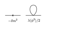
Figure 4: Mass counterterm and the one-loop diagram contributing to the thermal mass.

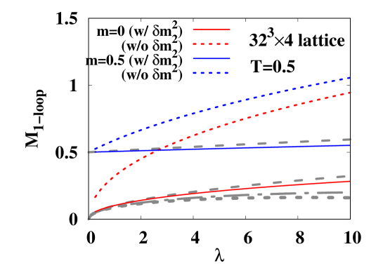
Figure 5: Thermal mass in $\phi^{4}$ theory on the lattice. Red and blue curves show the results of the thermal mass, $M=\omega(\bm{k}=\bm{0})$, with $m=0$ and $m=0.5$, respectively. Dotted and solid curves show the results without and with the counterterm, $\delta m^{2}$, respectively. Long-dashed, dot-dashed and short-dashed lines show the perturbative calculation results of the thermal mass in the continuum limit with the leading order ($M_{\mathrm{LO}}$), the resummed one loop ($M_{\mathrm{resum}}$) and the two loop ($M_{\mathrm{2{\operatorname{-}}loop}}$) effects, respectively.

In Fig. 5, we show the thermal mass calculated on a $32^{3}\times 4$ lattice at $T=0.5$. Thermal mass $M$ is obtained by solving Eqs. (65), (66) and (67) self-consistently by taking account of $M$ dependence of $\omega_{\bm{k}}$ and $\Omega_{\bm{k}}$. For comparison, we also show the results of the leading order estimate in the continuum and large $N$ limit, $1/a\to\infty$, $L\to\infty$ and $N\to\infty$ Kapusta ,

$$M_{\mathrm{LO}}^{2}=m^{2}+\lambda T^{2}/24.$$ (68)

For $m=0$, we also show the results with resummed one-loop contribution from the self-consistent treatment Kapusta ; TwoLoop ,

$$M^{2}_{\mathrm{resum}}=\frac{\lambda T^{2}}{24}\left[1-\frac{3}{\pi}\sqrt{\frac{\lambda}{24}}\right]\ ,$$ (69)

and the two-loop calculation result TwoLoop ,

$$M^{2}_{\mathrm{2{\operatorname{-}}loop}}= \frac{\lambda T^{2}}{24}\left\{1-\frac{3}{\pi}\sqrt{\frac{\lambda}{24}}+\frac{\lambda}{(4\pi)^{2}}\left[\frac{3}{2}\log\left(\frac{T^{2}}{4\pi\mu^{2}}\right)+2\log\left(\frac{\lambda}{24}\right)+\alpha\right]\right\}\ ,$$ (70)

where $\alpha=8.8865\ldots$, calculations is carried out at negligible $m/T$, and we take the renormalization scale as $\mu=2\pi T$. The obtained thermal mass on the lattice at $m=0$ is between $M_{\mathrm{LO}}$ and $M_{\mathrm{resum}}$. The deviation from $M_{\mathrm{resum}}$ may be due to the limited momentum range and the additional factor of $1/\sqrt{1+(\omega_{\bm{k}}/2\xi)^{2}}$ in $\left\langle{\phi^{2}}\right\rangle_{\mathrm{ren}}$ shown in Eq. (67).

4 Numerical results of replica evolution in scalar field theory

We shall now numerically evaluate the time evolution of replicas of classical field by using the replica Hamiltonian Eq. (36) defined in the 4D spacetime including the imaginary time. In order to examine the validity of replica evolution, we discuss the time-correlation function $C(t)$, which is the unequal-time two-point function at zero momentum. From the time correlation $C(t)$ obtained by the replica evolution, we extract the thermal mass $M$ and the damping rate $\gamma$, and compare them with the perturbative estimates.

4.1 Setup

We show the numerical results of time evolution of replicas on a $32^{3}\times 4$ lattice ($L=32,N=4$) at $T=0.5$ in the coupling range of $0.5\leq\lambda\leq 10$ with $m=0$ and $m=0.5$, as an example. The equation of motion is solved in the leap-frog method until $t=500$ with the time step of $\Delta t=0.025$ after the equilibration described below. When we take account of the mass renormalization, we subtract the divergent part of the induced mass by using the one-loop calculation results given in Eq. (66).

We prepare the initial condition by using the Langevin equation at the replica temperature of $\xi=NT=2$,

$$\frac{d\pi_{\tau{\bm{x}}}}{dt}=\frac{\partial\mathcal{H}}{\partial\phi_{\tau{\bm{x}}}}-\Gamma\pi_{\tau{\bm{x}}}+\sqrt{2\Gamma\xi}\,\zeta_{\tau{\bm{x}}}(t)\ ,$$ (71)

where the drift constant is taken to be $\Gamma=0.5$ and $\zeta_{\tau{\bm{x}}}(t)$ is the white noise, $\left\langle{\zeta_{\tau{\bm{x}}}(t)\,\zeta_{\tau^{\prime}\bm{x}}(t^{\prime})}\right\rangle=\delta_{\tau,\tau^{\prime}}\,\delta_{\bm{x},\bm{x}^{\prime}}\,\delta(t-t^{\prime})$. Since the relation of $\left\langle{\pi_{\tau{\bm{x}}}^{2}}\right\rangle=\xi$ should be satisfied in equilibrium, we rescale $\pi$ field at each step of the Langevin evolution. The equilibration time to prepare the initial condition is set to be $t_{\mathrm{eq}}=20$ in the lattice unit, which is found to be reasonably long in the coupling range for $\lambda\geq 4$. At smaller coupling, we take $\tau_{\mathrm{eq}}=100,60$ and $40$ for $\lambda=0.5,1$ and $2$, respectively.

It should be noted that any initial condition can be used, in principle, as long as the $\mathcal{H}$ distribution in the ensemble is consistent with that in equilibrium. Provided that the system is chaotic, all the phase-space points having the given $\mathcal{H}$ value are sampled in a long-time evolution Poincare . However, it generally takes more time for a Hamiltonian system to reach the equilibrium than in the Langevin equation. For example, the time needed to achieve equilibrium using the Langevin equation is found to be much shorter than the intrinsic relaxation time of the classical scalar field ($N=1$) in Ref. Matsuda . Thus it is expected that equilibrium configurations are efficiently obtained by using the Langevin equation.

We evaluate the time-correlation function $C(t)$ of the zero momentum component of the field variable, $\phi^{(i)}_{\tau,\bm{k}=\bm{0}}(t)=\sum_{\bm{x}}\phi^{(i)}_{\tau{\bm{x}}}(t)/\sqrt{L^{3}}$, with $i$ being the configuration index. The equilibrium average of the correlation function is obtained as the average over the replica ensemble, as shown in Eq. (64), where the replica ensemble is prepared by the Langevin equation discussed above. The number of replica configurations is taken to be $N_{\mathrm{conf}}=1000$. In order to reduce the statistical error, we also take average over the trigger time $t_{0}$.

With this setup, we have solved the time evolution of replica configurations, where the ensemble average should be consistent with the equilibrium expectation value. The ensemble average of $\pi_{\tau{\bm{x}}}^{2}$ is found to be $(0.1-0.2)\,\%$ larger than $\xi$ in the present setup. The overestimate can be suppressed with smaller drift coefficient and longer equilibration time, but it takes more time for the calculation and the above deviation would be small enough.

4.2 Momentum distribution and Rayleigh-Jeans divergence

Before discussing real time evolution, let us take a look at the thermal expectation value of the momentum distribution,

$$\left\langle{|\phi_{\bm{k}}|^{2}}\right\rangle= \frac{1}{N}\sum_{\tau}\left\langle{\phi_{\tau{\bm{k}}}\phi^{*}_{\tau{\bm{k}}}}\right\rangle=\frac{1}{N}\sum_{n}\left\langle{\phi_{{n\bm{k}}}\phi^{*}_{{n\bm{k}}}}\right\rangle\ ,$$ (72)

as a function of momentum $k=(\bar{\bm{k}}^{2})^{1/2}$. This appears in $\Delta=\left\langle{\phi^{2}}\right\rangle$ (Eq. (63)) and also in the energy in the form of $\omega_{\bm{k}}^{2}\left\langle{|\phi_{\bm{k}}|^{2}}\right\rangle=(m^{2}+k^{2})\left\langle{|\phi_{\bm{k}}|^{2}}\right\rangle$ in Eq. (49). In the free field case, the momentum distribution is given as

$$\left\langle{|\phi_{\bm{k}}|^{2}}\right\rangle= \frac{1}{\omega_{\bm{k}}\sqrt{1+(\omega_{\bm{k}}/2\xi)^{2}}}\left[\frac{1}{2}+\frac{1}{e^{\Omega_{\bm{k}}/T}-1}\right]\ ,$$ (73)

as discussed in Sec. 3.4. The first term in the bracket in Eq. (73) shows the zero point energy contribution which should be subtracted, and the second term shows the thermal part of the momentum distribution on the lattice which converges to the Bose-Einstein distribution function $1/[\exp(\omega_{\bm{k}}/T)-1]$ in the large $N$ limit. In Fig. 6, we show the replica ($N=4$) and classical field ($N=1$) ensemble results at $m=0$ and $\lambda=8$. We here adopt the thermal mass evaluated from the time-correlation function discussed later. These results agree with the free field results on the lattice. When the divergent part is subtracted (right panel), the momentum distributions approximately show exponential decay, as the Bose-Einstein distribution does. It may be interesting to find that even in the case of classical field, an approximate exponential decay is found, while the thermal part in the free field on the lattice deviate those in the large $N$ limit at high momenta, $k>1.5$. This approximate exponential decay comes from the decomposition of the divergent and finite parts as shown in Eq. (73). But this is not the end of the story.

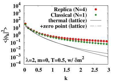
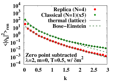
Figure 6: Momentum distribution $\left\langle{|\phi_{\bm{k}}|^{2}}\right\rangle$ obtained in replica ($N=4$, circles) and classical field ($N=1$, diamonds) ensembles at $m=0$ and $\lambda=2$ on the $32^{3}$ lattice in comparison with the thermal part of the distribution in the free field (solid curves). Filled and open symbols show the results at $t=t_{\mathrm{eq}}$ and $t=t_{\mathrm{eq}}+500$, respectively. Left panel shows the results including the zero point part, whose sum over the momenta diverges. Solid curves show the thermal part, and dash-dotted curves show the results including the zero point part. Right panel shows the results of the finite (renormalized) part of the momentum distribution, where the zero point part is subtracted. Solid curves show the thermal contribution on the lattice, and dashed curves show their large $N$ limit, $N\to\infty$, which is equivalent to the Bose-Einstein distribution multiplied by $1/\omega_{\bm{k}}$.

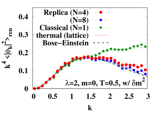
Figure 7: Renormalized momentum distribution multiplied by $k^{4}$, $k^{4}\left\langle{|\phi_{\bm{k}}|^{2}}\right\rangle_{\mathrm{ren}}$, obtained in replica ($N=4$, circles and $N=8$, squares) and classical field ($N=1$, diamonds) ensembles on the $32^{3}$ lattice at $m=0$, $\lambda=2$, and $T=0.5$. Solid curves show the thermal part of the distribution in the free field on the lattice, and the dashed curve shows the large $N$ limit, corresponding to the Bose-Einstein distribution multiplied by $k^{4}/\omega_{\bm{k}}$.

Next, let us discuss the Rayleigh-Jeans divergence. The momentum distribution appears in energy in the form of $k^{2}\left\langle{|\phi_{\bm{k}}|^{2}}\right\rangle$ and the number of momentum modes increase with the momentum as $k^{2}$. Thus the energy contains the kinetic energy part of $\int dkk^{4}\left\langle{|\phi_{\bm{k}}|^{2}}\right\rangle/2\pi^{2}$ in the continuum limit. In Fig. 7, we show the momentum distribution multiplied by $k^{4}$. We note that the classical field results ($N=1$) seem to saturate to a constant value. This behavior can be understood from the decomposition in Eq. (73). The thermal part in the decomposition in Eq. (73) is not necessarily exponentially suppressed but rationally suppressed at large $k$. Because of the functional form, $\mathrm{arcsinh}\,x=\log(\sqrt{1+x^{2}}+x)\simeq\log(2x)$ at large $x$, the “exponential” reads $\exp(-\Omega_{\bm{k}}/T)\simeq\exp(-2N\log(\omega_{\bm{k}}/NT))=(\omega_{\bm{k}}/NT)^{-2N}$ for large $\omega_{\bm{k}}$, $\omega_{\bm{k}}\gg\xi$. Then for high momentum, $k\gg m$ and $k\gg NT$, we find

$$\left\langle{|\phi_{\bm{k}}|^{2}}\right\rangle\simeq \frac{2NT}{k^{2}}\exp(-\Omega_{\bm{k}}/T)\to 2(NT)^{2N+1}k^{-2(N+1)}\ ,$$ (74)

$$k^{4}\,\left\langle{|\phi_{\bm{k}}|^{2}}\right\rangle\to \,2(NT)^{2N+1}k^{-2(N-1)}\ .$$ (75)

Then $k^{4}\left\langle{|\phi_{\bm{k}}|^{2}}\right\rangle$ converges to a constant with $N=1$. By substituting $T=0.5$ and $N=1$, the asymptotic value is found to be $2(NT)^{2N+1}=0.25$, which is close to the classical field results at large $k$. Thus we cannot fully remove the Rayleigh-Jeans divergence in the classical field in the present subtraction scheme without additional matching procedure.

In contrast, the replica results ($N=4$ and $N=8$) of the momentum distribution show suppressed behavior at high momentum as the Bose-Einstein distribution does, and $k^{4}\left\langle{|\phi_{\bm{k}}|^{2}}\right\rangle$ also decreases at large $k$. For the convergence of energy, $k^{4}\left\langle{|\phi_{\bm{k}}|^{2}}\right\rangle$ needs to converge to zero faster than $1/k$, then we find the constraint on $N$ as $2(N-1)>1$, or $N>3/2$. Thus we can expect that the integral would converge to a finite value also in the continuum limit, and the Rayleigh-Jeans divergence in energy can be fully removed in the replica evolution even with $N=4$. With $N=8$, the momentum distribution is closer to the Bose-Einstein distribution in the large $N$ limit.

4.3 Time-correlation function, thermal mass and damping rate

We now proceed to discuss the time-correlation function $C(t)$ obtained from the time evolution of replica ensemble. In Fig. 8, we show the time-correlation function $C(t)$ from replica evolution at $\lambda=2$ and $8$ with mass renormalization. We find that the time-correlation function is well described by the single damped oscillator $f_{1\omega}(t)$,

$$f_{1\omega}(t)=A\exp(-\gamma t)\,\cos(Mt+\delta)\ .$$ (76)

as shown by the thick blue curves.

Figure 8: Time-correlation function $C(t)$ in replica evolution on the $32^{3}\times 4$ lattice with $\lambda=2$ (left) and $8$ (right) with mass renormalization. Upper and lower panels show the results at $m=0.5$ and $m=0$, respectively. Replica evolution results (circles) are compared with the fitting results with $f_{1\omega}$ (thick blue curves).

We have obtained the thermal mass $M$ and the damping rate $\gamma$ by fitting the parameters $(M,\gamma,A,\delta)$ in $f_{1\omega}$ to $C(t)$ obtained from the replica evolution. In Fig. 9, we show the coupling dependence of the thermal mass $M$ obtained from the time-correlation function $C(t)$ in replica evolution without (left) and with (right) mass renormalization. We show the fitting results using the single oscillator function $f_{1\omega}$. The fitting results are close to the one loop calculation results without mass renormalization. With mass renormalization, the thermal mass is consistent with the one loop results at small coupling but considerably smaller than the one loop results in the strong coupling region. Replica evolution results at $m=0$ agree with the two loop results, while the classical field results ($N=1$) at $m=0$ show weaker reduction from the leading order results. Thus the replica evolution is expected to give higher order interaction effects over the one loop. For more serious comparison, we need to take account of two-loop counterterms of mass and coupling, and to choose the renormalization scale $\mu$ consistent with the present lattice calculation, but these are beyond the scope of this work.

Figure 9: Thermal mass $M$ obtained as the frequency of the time-correlation function $C(t)$ in replica evolution without (left) and with (right) mass counterterm at $m=0$ and $m=0.5$ (filled circles and squares). Diamonds show the results of classical field evolution ($N=1$) at $m=0$. Long-dashed, dot-dashed and short-dashed lines in the right panel show the perturbative calculation results with the leading order ($M_{\mathrm{LO}}$), the resummed one loop ($M_{\mathrm{resum}}$) and the two loop ($M_{\mathrm{2{\operatorname{-}}loop}}$) effects, respectively.

In Fig. 10, we show the damping rate $\gamma$ as a function of the coupling. We compare the replica evolution results with mass counterterm in comparison with the two loop calculation results TwoLoop ,

$$\gamma=\frac{\lambda^{2}T^{2}}{1536\pi M}\ ,$$ (77)

which is known to agree with the plasmon damping rate after the matching to quantum theory by substituting the leading order thermal mass estimate, $M_{\mathrm{LO}}=\sqrt{\lambda T^{2}/24}$. In this expression, the product $M\gamma$ is found to be independent of the mass.

Figure 10: Damping rate $\gamma$ multiplied by the mass $M$ obtained from the time-correlation function $C(t)$ in replica evolution with mass counterterm at $m=0$ and $m=0.5$ (circles and squares) in comparison with the two-loop calculation results (solid curves). Open and filled triangles show the results at $m=0$ obtained from the analyses of the Fourier transform of the time-correlation function using $\rho_{\Delta}$ and $f_{2\omega}$, respectively, as discussed in Appendix B. Open diamonds show the classical field results ($N=1$) at $m=0$.

The replica evolution results with $m=0.5$ seem to roughly agree with the perturbation calculation results in the small coupling region, and start to deviate from the perturbative estimate at larger coupling, $\lambda\geq 4$. Deviations at $\lambda\geq 4$ would be due to higher-order effects of the coupling, fluctuations, or the higher-momentum components ignored in the lattice discretization. With $m=0$, the damping rates are smaller than the perturbative estimate in the strong coupling region, as in the $m=0.5$ cases. At $\lambda\leq 4$, by comparison, the damping rate tends to be larger than the perturbative estimates. Since the thermal mass is small in this region of coupling, $M=0.085$ and $0.12$ at $\lambda=0.5$ and $1$, respectively, we may need larger size lattice. The apparent larger damping rate at small thermal mass may be related with the fragmentation of the single particle mode into several modes. The Fourier transform at small coupling and $m=0$ is found to be represented better by the superposition of several damped oscillators, each of which has a small width. If we adopt the width for each of the modes as the damping rate, the results at $\lambda=0.5$ and $1$ agree with the perturbative estimates as shown by open triangles in Fig. 10. The analysis of the Fourier transform is given in Appendix B. It should be also noted that the classical field results roughly agree with the perturbative calculation, as already noted in previous works Aarts ; Aarts:2001yn ; Aarts-spec .

Before closing this section, we would like to mention that $C(t)$ is the time-symmetric part of the two-point function, $C(-t)=C(t)$, whose transformation is referred to as the statistical function. In quantum field theory, the spectral function is more important, but we need to evaluate the commutator of unequal-time field variables by using, for example, the Poisson bracket Aarts-spec . We show the time-odd part of the time-correlation function in a harmonic oscillator in Appendix C, but we leave evaluating the spectral function in field theories in the future work.

5 Summary and perspectives

We have investigated the simultaneous real-time evolution of several classical field configurations, referred to as replicas, which interact with the nearest neighbor replicas with a specific form of interaction, the $\tau$-derivative term. Classical evolution of replica ensemble is found to provide the correct quantum field partition function in equilibrium. The average of field variables over replica indices approximately obeys the classical field equation of motion when the fluctuations among the replicas are small. The exponential suppression factor of high momentum modes appears from the sum over the replica index, which can be regarded as the imaginary time, provided that the zero point energy contribution is subtracted. We have examined the behavior of the time-correlation function (the unequal-time two-point function) at zero momentum without and with the mass counterterm. The time-correlation function in the replica evolution is expected to show oscillatory behavior with the frequency of the thermal mass $M$ at temperatures $T/M\gtrsim 0.5$, as demonstrated in the quantum mechanics of the harmonic oscillator. The time-correlation function in the $\phi^{4}$ theory seems to show reasonable behavior: The thermal mass of the zero momentum mode roughly agrees with the perturbative calculation results at small coupling. Thus the replica evolution should be useful to describe real-time behavior in equilibrium.

It would be desired to further examine the replica evolution as a candidate of the frameworks to describe non-equilibrium real-time quantum-field evolution. As long as the distribution of initial replica Hamiltonian values is properly given, distribution of field variables in replica ensemble should finally relax to the correct quantum statistical distribution, even if one starts from far-from-equilibrium configurations. In discussing non-equilibrium real-time evolution, however, it would be necessary to introduce additional time scale. It should be noted that replica evolution is conjectured to be useful in a heuristic context, but it is not derived based on some principle. Thus formal derivation or justification is desired. For example, the equivalence between the classical field theory and the Boltzmann equation Mueller:2002gd would be a good guide for the formal discussions. It is also interesting to discuss, for example, the $O(N)$ model, where there exist results of dynamical calculations using the two particle irreducible (2PI) effective action Berges:2004yj ; Aarts:2001yn .

Once the present framework is proven to be useful in describing quantum field evolution toward equilibrium, application to the Yang-Mills field is another important subject to study. The temporal component of the vector field is usually Wick rotated in the imaginary time formalism and we cannot apply the replica evolution as it is. However, spatial components are the same in the imaginary and real time formalism and we can apply the replica evolution. Thus it is possible to examine the replica evolution of classical Yang-Mills field in the temporal gauge where the temporal components of the vector field are set to be zero. Then it is interesting to examine whether or not the quantum statistical features affect the dynamical evolution in the initial stage of high-energy heavy-ion collisions. In order to describe inhomogeneous and nonequilibrium evolution, it is necessary to take account of spacetime dependence of temperature, which may need to invoke the nonequilibrium statistical operator (NSO) method NSO . In the NSO method, the inverse temperature and several other variables are introduced as the local conjugate fields of the corresponding density fields, and are determined by the time evolution and the initial condition under the assumption that the local Gibbs distribution in the initial state. Combining the NSO method and the replica evolution may be a challenging but valuable subject to study.

Appendix A Matsubara frequency summation

In deriving Eq. (52), we have used the Matsubara frequency summation formulae,

$$S=T\sum_{n}g(\omega_{n}=2\pi nT)=-i\sum_{\omega_{0}}\frac{\mathrm{Res}\,g(\omega_{0})}{e^{i\omega_{0}/T}-1}\ ,$$ (78)

where $g(\omega)$ is an analytic function of $\omega$, does not have poles on the real axis, and decreases faster than $1/\omega$ at $\omega\to\infty$, i.e. $\lim_{|\omega|\to\infty}\omega g(\omega)=0$. The poles and residues of $g(\omega)$ are denoted by $\omega_{0}$ and $\mathrm{Res}\,g(\omega_{0})$.

Specifically, we consider the following sum

$$S=\frac{1}{N}\sum_{n}\log\left[E^{2}+\sin^{2}(\omega_{n}/2)\right]\ ,$$ (79)

where $T=1/N$ and $\omega_{n}=2\pi n/N$. The derivative $dS/dE$ is in the form of Eq. (78),

$$\frac{dS}{dE}= \frac{1}{N}\sum_{n}\frac{2E}{E^{2}+\sin^{2}(\omega_{n}/2)}\ ,$$ (80)

where $g(\omega)=2E/(E^{2}+4\sin^{2}(\omega/2))$ and $T=1/N$. The poles and residues of $g(\omega)$ are found to be $i\omega_{0}=\pm\Omega=\pm 2\mathrm{arcsinh}\,E$ and $\mathrm{Res}\,g(\omega_{0})=\pm 2i/\sqrt{1+E^{2}}$, so $dS/dE$ is obtained as

$$\frac{dS}{dE}= \frac{2}{\sqrt{1+E^{2}}}\,\frac{e^{N\Omega}+1}{e^{N\Omega}-1}=\frac{2\coth(N\Omega/2)}{\sqrt{1+E^{2}}}\ .$$ (81)

By integration, the sum in Eq. (79) is found to be

$$S= \frac{2}{N}\log\left[\sinh(N\Omega/2)\right]+\mathrm{const.}\ .$$ (82)

The constant can be fixed as $2\log 2(1/N-1)$ by considering the large $E$ limit of $S$, $S=2\log{E}+\mathcal{O}(1/E)$. By substituting $E=\omega_{\bm{k}}/2\xi$, we obtain Eq. (52).

The same formula can be used to obtain $\Delta=\left\langle{\phi^{2}}\right\rangle$ in Eq. (63).

$$\Delta_{\bm{k}}= \frac{1}{4\xi}\frac{1}{N}\sum_{n}\frac{1}{(\omega_{\bm{k}}/2\xi)^{2}+\sin^{2}(\omega_{n}/2)}=\frac{1}{4\xi}\frac{\coth(\Omega_{\bm{k}}/2T)}{(\omega_{\bm{k}}/2\xi)\sqrt{1+(\omega_{\bm{k}}/2\xi)^{2}}}$$

$$= \frac{1}{L^{3}}\frac{1}{\omega_{\bm{k}}\sqrt{1+(\omega_{\bm{k}}/2\xi)^{2}}}\left[\frac{1}{2}+\frac{e^{-\Omega_{\bm{k}}/T}}{1-e^{-\Omega_{\bm{k}}/T}}\right]\ ,$$ (83)

where $\Omega_{\bm{k}}=2\xi\mathrm{arcsinh}(\omega_{\bm{k}}/2\xi)$. Then we can obtain $\Delta=\left\langle{\phi^{2}}\right\rangle=\sum_{\bm{k}}\Delta_{\bm{k}}/L^{3}$ in Eq. (63).

Appendix B Fourier transform of time-correlation function

In Sec. 4, the damping rate is found to be larger in the weak coupling region with mass counterterm at $m=0$. Here we would like to discuss this point by using the Fourier transform of the time-correlation function,

$$\rho(\omega)\equiv\frac{1}{2}\int_{-\infty}^{\infty}dte^{i\omega t}C(|t|).$$ (84)

In Fig. 11, we show $\rho(\omega)$ obtained from the replica evolution with mass counterterm at $\lambda=0.5$ and $8$ with $m=0$ in comparison with the Fourier transform of the fitting function $f_{1\omega}$. At $\lambda=0.5$, the spectrum has a peak having the width of the order of $10^{-2}$, but the tails fall off much faster than the behavior expected from the width or the damping rate from the fitting function $f_{1\omega}$, $\gamma\simeq 2.6\times 10^{-3}$.

Figure 11: Fourier transform of the time-correlation function. We show the results with mass counterterm at $\lambda=0.5$ (left) and $8$ (right) with $m=0$. Histograms show the Fourier transform of $C(t)$ obtained from the replica evolution. Solid, dashed and dotted curves show the Fourier transform $\rho_{\Delta}(\omega)$ and the Fourier transform of $f_{1\omega}$ and $f_{2\omega}$, respectively.

One of the possible interpretations of this spectrum is to consider that there are several modes, each of which has a small damping rate but has a mass spread in the region with $10^{-2}$ width. As an attempt, we use the two damped oscillator functions, where the two frequencies are close to each other,

$$f_{2\omega}(t)= A\exp(-\gamma t)\left\{r\cos[(\omega+\delta\omega)t+\delta]+(1-r)\cos[(\omega-\delta\omega)t+\delta]\right\}\ .$$ (85)

The dotted lines show the Fourier transform of $f_{2\omega}$ fitted to $C(t)$. The tail region is found to be suppressed, but not enough at $\lambda=0.5$. Next, we consider the following fitting function, convolution of the step function and the Lorentzian, for the Fourier transform,

$$\rho_{\Delta}(\omega)= \frac{A}{2\Delta}\int_{M-\Delta}^{M+\Delta}\,\frac{\gamma dM^{\prime}}{(\omega-M^{\prime})^{2}+\gamma^{2}}$$

$$= \frac{A}{2\Delta}\left[\arctan\left(\frac{\omega-M+\Delta}{\gamma}\right)-\arctan\left(\frac{\omega-M-\Delta}{\gamma}\right)\right].$$ (86)

The fitting results are shown by the solid curves, which shows both wide width of the peak and the fast fall off. The damping rate of each mode becomes smaller, $\gamma\simeq 1.5\times 10^{-4}$, and roughly agrees with the perturbative estimate, as shown by open triangles in Fig. 10.

At larger coupling, fitting results of the damping rate with $f_{1\omega}$, $f_{2\omega}$ and $\rho_{\Delta}$ are consistent, and the peak part of the spectrum is reproduced in these functions, as shown in the right panel of Fig. 11.

Appendix C Time-odd part of the time-correlation function in harmonic oscillator

While the expectation value of symmetrized (Weyl ordered) product can be obtained in classical dynamics, we need additional care to evaluate the expectation value of the anti-symmetrized product such as the commutator. For example, the time-odd part of the time-correlation function may be obtained by using the quantum-classical correspondence for the commutator Aarts-spec ,

$$[A,B]\to i\hbar\{A,B\}_{\mathrm{PB}}+\mathcal{O}(\hbar^{3})\ ,$$ (87)

where we explicitly show $\hbar$ here and $\{A,B\}_{\mathrm{PB}}$ is the Poisson bracket. If we ignore $\mathcal{O}(\hbar^{3})$, the time-odd part of the time-correlation function would be obtained as

$$\left\langle{\frac{1}{2}[\hat{x}_{H}(t),\hat{x}_{H}(0)]}\right\rangle_{T}\simeq \left\langle{\frac{i}{2}\{x(t),x(0)\}_{\mathrm{PB}}}\right\rangle=\frac{i}{2}\left\langle{\sum_{\tau,\tau^{\prime}}\left[\frac{\partial x_{\tau}(t)}{\partial x_{\tau^{\prime}}(t_{0})}\frac{\partial x_{\tau}(0)}{\partial p_{\tau^{\prime}}(t_{0})}-\frac{\partial x_{\tau}(t)}{\partial p_{\tau^{\prime}}(t_{0})}\frac{\partial x_{\tau}(0)}{\partial x_{\tau^{\prime}}(t_{0})}\right]}\right\rangle$$

$$= \frac{i}{2}\left\langle{\sum_{n,n^{\prime}}\left[\frac{\partial\bar{x}_{n}(t)}{\partial\bar{x}_{n^{\prime}}(t_{0})}\frac{\partial\bar{x}_{n}(0)}{\partial\bar{p}_{n^{\prime}}(t_{0})}-\frac{\partial\bar{x}_{n}(t)}{\partial\bar{p}_{n^{\prime}}(t_{0})}\frac{\partial\bar{x}_{n}(0)}{\partial\bar{x}_{n^{\prime}}(t_{0})}\right]}\right\rangle$$

$$= -\frac{i}{2}\sum_{n}\frac{1}{M_{n}}\sin M_{n}t\ .$$ (88)

Since the Fourier transformation and the time evolution are the canonical transformation, we can choose either $(x_{\tau},p_{\tau})$ or $(\bar{x}_{n},\bar{p}_{n})$ in calculating the Poisson bracket and the time $t_{0}$ should be arbitrary. The zero Matsubara frequency contribution in Eq. (88) agrees with the quantum mechanical result.

In the case of coupled oscillators such as the field theories, it is in principle possible to calculate the Poisson bracket of the unequal-time observables by using the Hessian matrix Entropy , while it requires to store the matrix elements of degrees of freedom squared, $(2N_{\mathrm{dof}})^{2}$ with $N_{\mathrm{dof}}=NL^{3}$ for one component scalar field theory on the $L^{3}\times N$ lattice. We also need to multiply the matrix at each step of time, so the numerical cost is much larger than the time-correlation function discussed in this article.

References

- (1) E. P. Gross, Il Nuovo Cimento 20, 454 (1961); L. P. Pitaevskii, Sov. Phys. JETP 13, 451 (1961); P. Muruganandam, S. K. Adhikari, Comp. Phys. Comm. 180, 1888 (2009).
- (2) D. J. Thouless and J. G. Valatin, Nucl. Phys. 31 211 (1962); A. D. McLachlan and M. A. Ball, Rev. Mod. Phys. 36, 844 (1964); Y. M. Engel, D. M. Brink, K. Goeke, S. J. Krieger, D. Vautherin, Nucl. Phys. A 249, 215 (1975).
- (3) K. Sato, Mon. Notices Royal Astron. Soc. 195, 467 (1981); A. H. Guth, Phys. Rev. D 23, 347 (1981).
- (4) S. Y. Khlebnikov and I. I. Tkachev, Phys. Rev. Lett. 77, 219 (1996).
- (5) L. D. McLerran and R. Venugopalan, Phys. Rev. D 49, 2233 (1994). P. Romatschke and R. Venugopalan, Phys. Rev. Lett. 96, 062302 (2006); T. Lappi and L. McLerran, Nucl. Phys. A 772, 200 (2006); J. Berges, S. Scheffler and D. Sexty, Phys. Rev. D 77, 034504 (2008); K. Fukushima and F. Gelis, Nucl. Phys. A 874, 108 (2012). T. Epelbaum and F. Gelis, Phys. Rev. Lett. 111, 232301 (2013).
- (6) A. Dumitru and Y. Nara, Phys. Lett. B 621, 89 (2005); A. Dumitru, Y. Nara and M. Strickland, Phys. Rev. D 75, 025016 (2007).
- (7) S. G. Matinyan, E. B. Prokhorenko and G. K. Savvidy, JETP Lett. 44, 138 (1986); B. Müller and A. Trayanov, Phys. Rev. Lett. 68, 3387 (1992).
- (8) T. Kunihiro, B. Muller, A. Ohnishi, A. Schafer, T. T. Takahashi and A. Yamamoto, Phys. Rev. D 82, 114015 (2010); H. Iida, T. Kunihiro, B. Mueller, A. Ohnishi, A. Schaefer and T. T. Takahashi, Phys. Rev. D 88, 094006 (2013); H. Tsukiji, H. Iida, T. Kunihiro, A. Ohnishi and T. T. Takahashi, Phys. Rev. D 94, 091502 (2016); H. Tsukiji, T. Kunihiro, A. Ohnishi and T. T. Takahashi, PTEP 2018, 013D02 (2018).
- (9) M. M. Homor and A. Jakovac, Phys. Rev. D 92, 105011 (2015);
- (10) H. Matsuda, T. Kunihiro, A. Ohnishi, T. T. Takahashi, PTEP 2020, 053D03 (2020); H. Matsuda, T. Kunihiro, A. Ohnishi, T. T. Takahashi, arXiv:2007.06886 [hep-ph].
- (11) A. A. Vlasov, J. Exp. Theor. Phys. 8, 291 (1938); Soviet Physics Uspekhi, 10, 721 (1968).
- (12) John von Neumann, Göttinger Nachrichten 1, 245 (1927).
- (13) E. Wigner, Phys. Rev. 40, 749 (1932).
-
(14)
N. Rostoker and M. N. Rosenbluth, Phys. Fluids 3, 1 (1960);
C. Y. Wong, Phys. Rev. C 25, 1460 (1982). - (15) D. Bodeker, L. D. McLerran and A. V. Smilga, Phys. Rev. D 52, 4675 (1995).
- (16) C. Greiner and B. Muller, Phys. Rev. D 55, 1026 (1997).
- (17) G. Aarts and J. Smit, Phys. Lett. B 393, 395 (1997); Nucl. Phys. B 511, 451 (1998); G. Aarts, G. F. Bonini and C. Wetterich, Phys. Rev. D 63, 025012 (2001).
- (18) J. Berges, AIP Conf. Proc. 739, 3 (2004).
- (19) G. Aarts and J. Berges, Phys. Rev. Lett. 88, 041603 (2002).
- (20) Y. Hatta and A. Nishiyama, Nucl. Phys. A 873, 47 (2012).
- (21) E. A. Uehling and G. E. Uhlenbeck, Phys. Rev. 43, 552 (1933); G. F. Bertsch and S. Das Gupta, Phys. Rept. 160, 189 (1988); A. Ono, H. Horiuchi, T. Maruyama and A. Ohnishi, Phys. Rev. Lett. 68, 2898 (1992); Prog. Theor. Phys. 87, 1185 (1992); A. Ohnishi and J. Randrup, Phys. Rev. Lett. 75, 596 (1995); Phys. Lett. B 394, 260 (1997); A. Ono and H. Horiuchi, Phys. Rev. C 53, 2958 (1996); Y. Hirata, Y. Nara, A. Ohnishi, T. Harada and J. Randrup, Prog. Theor. Phys. 102, 89 (1999); P. Chomaz, M. Colonna and J. Randrup, Phys. Rept. 389, 263 (2004).
-
(22)
G. Parisi and Y. s. Wu,
Sci. Sin. 24, 483 (1981);
G. Parisi,
Phys. Lett. 131B, 393 (1983);
P. H. Damgaard and H. Huffel, Phys. Rept. 152, 227 (1987). - (23) S. Duane, A. D. Kennedy, B. J. Pendleton and D. Roweth, Phys. Lett. B 195, 216 (1987).
- (24) J. I. Kapusta and C. Gale, ”Finite-temperature field theory: Principles and applications” (Cambridge University Press, Cambridge, 2006).
- (25) R. R. Parwani, Phys. Rev. D 45, 4695 (1992) Erratum: [Phys. Rev. D 48, 5965 (1993)].
- (26) H. Poincaré, Acta Math. 13, 1 (1890).
- (27) G. Aarts, Phys. Lett. B 518, 315 (2001).
- (28) A. H. Mueller and D. T. Son, Phys. Lett. B 582, 279 (2004).
- (29) D. N. Zubarev, A. V. Prozorkevich, and S. A. Smolyanskii, Theor. Math. Phys. 40, 821 (1979); F. Becattini, L. Bucciantini, E. Grossi, and L. Tinti, Eur. Phys. J. C 75, 191 (2015); S.-i. Sasa, Phys. Rev. Lett. 112, 100602 (2014); T. Hayata, Y. Hidaka, T. Noumi and M. Hongo, Phys. Rev. D 92, 065008 (2015).