Sparse Grids based Adaptive Noise Reduction strategy for Particle-In-Cell schemes

Abstract

We propose a sparse grids based adaptive noise reduction strategy for electrostatic particle-in-cell (PIC) simulations. Our approach is based on the key idea of relying on sparse grids instead of a regular grid in order to increase the number of particles per cell for the same total number of particles, as first introduced in [1]. Adopting a new filtering perspective for this idea, we construct the algorithm so that it can be easily integrated into high performance large-scale PIC code bases. Unlike the physical and Fourier domain filters typically used in PIC codes, our approach automatically adapts to mesh size, number of particles per cell, smoothness of the density profile and the initial sampling technique. Thanks to the truncated combination technique [2, 3, 4], we can reduce the larger grid-based error of the standard sparse grids approach for non-aligned and non-smooth functions. We propose a heuristic based on formal error analysis for selecting the optimal truncation parameter at each time step, and develop a natural framework to minimize the total error in sparse PIC simulations. We demonstrate its efficiency and performance by means of two test cases: the diocotron instability in two dimensions, and the three-dimensional electron dynamics in a Penning trap. Our run time performance studies indicate that our new scheme can provide significant speedup and memory reduction as compared to regular PIC for achieving comparable accuracy in the charge density deposition.

1 Introduction

Particle-in-cell (PIC) schemes have been a popular and effective method for the simulation of kinetic plasmas for a long period of time [5, 6, 7]. Compared to continuum kinetic codes, PIC schemes effectively reduce the dimension from six to three for three-dimensional simulations whereas compared to pure particle codes with direct summation it reduces the computation of self-consistent forces from $\mathcal{O}(N_{p}^{2})$ to $\mathcal{O}(N_{p}+N_{c})$ where $N_{p}$ is the total number of particles and $N_{c}\ll N_{p}$ is the number of mesh points. Even though the fast multipole method [8] reduces the complexity of pure particle schemes to $\mathcal{O}(N_{p})$, such an approach has other limitations such as the need for overly restrictive small time stepsizes. The other attractive features of PIC schemes include simplicity, ease of parallelization and robustness for wide variety of physical scenarios [1].

The main drawback of PIC schemes as compared to deterministic continuum kinetic schemes is the numerical error associated with particle noise, which decreases slowly as one increases the number of particles. Specifically, the noise in PIC schemes decreases as $1/\sqrt{P_{c}}$ where $P_{c}=N_{p}/N_{c}$ is the number of particles per cell. High fidelity large-scale 3D PIC simulations thus often require at least $\mathcal{O}(10^{9})$ grid points and $\mathcal{O}(10^{12})$ particles to get the desired accuracy level [9]. These simulations require hours to complete even on large-scale state-of-the-art supercomputers available today. Thus, noise reduction approaches are of great interest to the PIC community to improve accuracy and also to speed up the computations and reduce memory requirements.

There have been several efforts in this area over the past years and a brief overview is given in section 3. Some of the strategies such as the $\delta f$ technique [10, 11, 12] are applicable for certain classes of plasma physics problems and give great computational savings whereas for others they are not obvious to apply. Filtering is a common noise reduction technique which finds applications in many production-level PIC codes such as TRISTAN-MP [13, 14], ORB5 [15], IMPACT-T [16] and Warp-X [17], to name a few. One of the primary reasons for it is its simplicity and ease of implementation in these frameworks. The stencil width and number of passes in case of digital filters and the cut-off wavenumber in case of Fourier domain filters is typically selected based on experience and knowledge about the physical problem at hand. Thus these could result in scenarios where either too much signal is smoothed or the high frequency noise is not removed sufficiently. Even if we managed to choose the parameters in the filter so that they are optimal for a particular mesh size, number of particles per cell, time instant/smoothness of the function and the initial sampling technique they may no longer be optimal once we change any of the above and require tuning once again.

Our objective in this work is to develop a noise reduction strategy, or filtering scheme, that automatically adapts itself to the aforementioned parameters. Just like other filtering techniques we also want it to be easily integrated into existing production-level PIC codes. Towards that goal, we adopt a key idea introduced in the recent work [1] which combined sparse grids with the PIC scheme. In that article, the authors showed that owing to the large cell sizes involved in sparse grids compared to regular grids, the PIC scheme combined with sparse grids has many more particles per cell than its regular counterpart. This led to significant noise reduction and enormous speedups for certain classes of problems which have smooth or axis-aligned density profiles.

Let us give a brief overview of the present work. By re-visiting the idea introduced in [1] from a filtering perspective, we first construct a sparse grids based noise reduction strategy for electrostatic PIC simulations. Compared to existing filtering approaches, this sparse grids based approach is superior for functions which are smooth or aligned with an axis. In simple terms this can be understood as follows: with any filtering technique the reduction in noise comes with a price, which is an increase in the grid-based error. In case of the sparse grids filtering, the noise reduction is maximal due to the least number of grid points involved in the approximation which translates to maximum particles per cell in the context of PIC. At the same time the increase in grid-based error for smooth or axis-aligned functions is minimal. However, the same cannot be said for other functions in general and in those cases the increase in grid-based error associated with sparse grids is high. In order to tackle that issue, we use the so-called truncated combination technique [2, 3, 4], which reduces the large grid-based error of standard sparse grids technique for non-aligned and non-smooth functions. This is because the truncated combination technique uses a different choice of coarse grids with finer mesh sizes than those used in the standard sparse grid combination. The truncation parameter involved in the combination technique is crucial for minimizing the sum of grid-based error and particle noise. Hence, we propose a heuristic based on formal error analysis to calculate the optimal truncation parameter on the fly which minimizes the total error.

This paper is organized as follows. Section 2 introduces the PIC method in the context of electrostatic Vlasov-Poisson equations. Section 3 briefly reviews the existing noise reduction strategies in PIC and provides motivation and objectives for this article. Section 4 explains in detail the components and algorithm for the sparse grids based noise reduction strategy. Numerical results for the 2D diocotron test case and 3D penning trap are presented in section 5 and section 6 presents the conclusions and future work.

2 Particle-in-cell method

In this work, we consider the non-relativistic electrostatic Vlasov-Poisson system with a fixed magnetic field, and introduce the PIC method in that setting. The electrons are immersed in a uniform, immobile, neutralizing background ion population and the system is given by

$$\frac{\partial f}{\partial t}+\mathbf{v}\cdot\nabla_{{\bf x}}f+\frac{q_{e}}{m_{e}}\left(\mathbf{E}+\mathbf{v}\times\mathbf{B}_{ext}\right)\cdot\nabla_{\mathbf{v}}f=0,$$ (1)

where $\mathbf{E}=\mathbf{E}_{sc}+\mathbf{E}_{ext},$ and the self-consistent fields due to space charge are given by

$$\mathbf{E}_{sc}=-\nabla\phi,\quad-\Delta\phi=\rho=\rho_{e}-\rho_{i}.$$

In the above equation $f({\bf x},\mathbf{v},t)$ is the electron phase-space distribution, $q_{e}$ and $m_{e}$ are the electron charge and mass respectively. The total electron charge in the system is given by $Q_{e}=q_{e}\int\int fd{\bf x}d\mathbf{v}$, the electron charge density by $\rho_{e}({\bf x})=q_{e}\int fd\mathbf{v}$ and the constant ion density by $\rho_{i}=\frac{Q_{e}}{\int d{\bf x}}$. Throughout this paper we use bold letters for vectors and non-bold ones for scalars.

The particle-in-cell method discretizes the phase space distribution $f({\bf x},\mathbf{v},t)$ in a Lagrangian way by means of macro-particles (hereafter referred to as particles for simplicity). At time $t=0$, the distribution $f$ is sampled to get the particles and after that a typical computational cycle in PIC consists of the following steps:

1. Assign a shape function e.g., cloud-in-cell [6] to each particle $p$ and deposit the electron charge onto an underlying mesh.

2. Use a grid-based Poisson solver to compute $\phi$ by solving $-\Delta\phi=\rho$ and differentiate $\phi$ to get the electric field $\mathbf{E}=-\nabla\phi$ on the mesh.

3. Interpolate $\mathbf{E}$ from the grid points to particle locations ${\bf x}_{p}$ using the same interpolation function as used for the charge deposition in step 1.

4. By means of a time integrator advance the particle positions and velocities using

   $$\frac{d\mathbf{v}_{p}}{dt} =\frac{q_{e}}{m_{e}}\left(\mathbf{E}+\mathbf{v}\times\mathbf{B}_{ext}\right)|_{{\bf x}={\bf x}_{p}},$$

   $$\frac{d{\bf x}_{p}}{dt} =\mathbf{v}_{p}.$$

The sources of different errors in the PIC simulations and their order of accuracies for typical choices are as follows. For simplicity if we consider a uniform mesh with spacing $h$ in all the directions then for the shape functions used in typical PIC schemes (B-splines), the grid-based error scales as $\mathcal{O}(h^{2})$. This is a result of approximating $\delta$ functions in the configuration space by shape functions of compact support. The Poisson equation is typically solved by means of FFT solvers or by multigrid methods. In case of multigrid solvers the equation is discretized by second-order finite difference or finite element schemes. The field solves together with the interpolation (typically linear) accounts for an additional $\mathcal{O}(h^{2})$. The particle noise is the result of approximating the expected value of the shape function by an arithmetic mean over a finite number of discrete particles. It scales as $(N_{p}h^{d})^{-1/2}$ [1], where $d$ is the spatial dimension of the problem. The initial distribution is sampled using one of the standard sampling techniques such as the naive Monte-Carlo strategy [11], importance sampling [11] or by means of the quiet start [18, 19, 20]. The choice of initial sampling plays an important role in determining the constant associated with the particle noise. Finally, for time integration usual choices are the second-order leap frog scheme [6] and Runge-Kutta schemes of order 2 and higher. If we consider the leap frog scheme then the error in the time discretization scales as $\mathcal{O}(\Delta t^{2})$. The mesh size $h$, time step $\Delta t$ and the number of particles $N_{p}$ in most PIC simulations are such that the dominant error comes from the particle noise. Hence, high fidelity simulations typically require a large number of particles to minimize it. The high noise associated with PIC simulations motivated researchers to develop several noise reduction strategies which we will discuss next.

3 Noise reduction strategies in PIC

Noise reduction can be achieved in several ways in the context of PIC simulations and they can be categorized as: (i) variance reduction techniques such as the $\delta f$ method [10, 11, 12] and quiet start [12]; (ii) phase space remapping [18, 19, 20]; (iii) filtering in physical domain [6, 21, 13, 14, 22], Fourier domain [6, 15] and wavelet domain [23, 16, 24]. The list is not exhaustive and there are many other contributions in this area. In addition, recently a noise reduction strategy using kernel density estimation algorithm has been proposed in [25], where the authors adaptively select the shape functions in PIC which minimize the sum of bias squared and variance of the error in the density. Also, in [1] sparse grid techniques are used to achieve noise reduction in PIC, as we will explain in detail in the next section since our work is based on this strategy. In this section, we will focus more on the filtering strategies due to their relevance in the context of our work.

The goal of filtering in PIC simulations is to smooth high frequency oscillations usually associated with noise. Filtering can be done in any field quantity, although the most common one in electrostatic PIC is the charge density [21] as it is the origin of noise and the potential and electric field are smoother because of the integration involved in solving Poisson’s equation. In case of filtering in the physical domain, one typically selects a filter of certain stencil width e.g., binomial filter, and does few passes on the field quantity. On the other hand for filters in the Fourier domain a maximum wavenumber is specified by the user and the filter eliminates all the wavenumbers higher than the specified cut-off wavenumber [6]. In almost all the filtering strategies, the number of passes/stencil width in the physical domain or the cut-off wavenumber in the Fourier domain has to be chosen a priori such that the total error, which is the sum of grid-based error (bias) and particle noise (variance) is minimized. However, in practice there are not many constructive strategies available to pick these parameters and in many cases the values are chosen based on rule of thumb and previous experiences [26]. If we managed to choose these parameters so that they are optimal for a particular time instant, mesh, number of particles per cell and sampling technique, they are unlikely to remain so as the simulation evolves. Indeed, due to non-linear space charge effects fine scale structures appear in the density and this changes the smoothness of the profile continuously with time. Hence an ideal filter should be adaptive with respect to all aforementioned parameters to minimize the total error.

Our objective is to develop a noise reduction strategy for PIC simulations which automatically adapts with respect to time, mesh size, number of particles per cell and the initial sampling technique. Since our ultimate goal is large-scale 3D high fidelity plasma simulations we also want the approach to be scalable in high performance computing architectures. Finally, it would be desirable if the strategy integrates well with the existing high performance large-scale PIC code bases such as OPAL [27] so that the user community of these codes can benefit from it. Towards these goals, we propose a sparse grids based adaptive noise reduction strategy in the following section.

4 Sparse grids based noise reduction

The sparse grid combination technique was first introduced in [28] as a way to approximate smooth functions on rectangular grids efficiently, by a specific linear combination of their approximations on different coarse grids. If we consider linear interpolation as an example, then for a regular grid of mesh size $h$ we need $\mathcal{O}(h^{-d})$ grid points to get an accuracy of $\mathcal{O}(h^{2})$. The sparse grid combination technique on the other hand uses only $\mathcal{O}(h^{-1}|log(h)|^{(d-1)})$ total number of points to get an accuracy of $\mathcal{O}(h^{2}|log(h)|^{(d-1)})$ for smooth functions, which is only slightly deteriorated compared to the regular grids. Thus we can clearly see the advantages of sparse grids in high dimensions and it is mainly used to tackle the curse of dimensionality in many applications [29]. The key idea is the cancellations that happen between the error expansions in the different coarse grids, which are called component grids in the sparse grids terminology. Also, the scalar values that multiply each component grid involved in the combination are called the combination coefficients. In Figure 1 an illustration is shown, where we can see the different component grids and their combination coefficients involved in approximating a $2^{8}\times 2^{8}$ regular grid. The literature on sparse grid combination technique and sparse grids in general is vast and the readers can refer to [29, 28, 30, 31, 32] and the references therein for more details.

In [1], the authors combined sparse grid combination technique with the PIC method and showed noise reduction and order of magnitude speedups for a certain class of problems. One of the key ideas from [1] is that for the same total number of particles $N_{p}$, sparse grids have many more particles per cell compared to regular grids and hence significantly less noise. However, this comes with a limitation which is explained as follows. While for smooth functions (Figure 2(d)) or functions aligned with an axis (Figure 10(d)) the increase in grid-based error for using sparse grids is very small in comparison to regular grids, for non-smooth or non-aligned functions (Figures 2(f), 10(e) and 10(f)) the increase is much higher [33]. Hence, the sparse PIC proposed in [1] showed large speedups and memory savings for smooth functions, whereas for ones with fine scale structures that are not aligned with the grid the regular PIC itself was more advantageous. The sparse PIC for these cases seemed to provide benefits only in the limit of asymptotically fine meshes at least for two-dimensional problems where the weaker dependence of the computational cost on dimension is not as noticeable.

We base our work on the key idea of increased particles per cell in sparse grids shown in [1] compared to regular grids for the same total number of particles $N_{p}$. However, in this paper we provide the following novelties and improvements compared to [1].

Firstly, the sparse PIC scheme in [1] performs all the operations e.g., charge deposition and Poisson solve on the sparse grids and does not introduce regular grids at all except for visualization purposes or post-processing. By contrast in the current approach we use sparse grids only for noise reduction in the charge density while all the operations such as charge deposition and Poisson solve happen in the regular grid just like in usual PIC codes.

The reason for pursuing this approach is that we want our strategy to fit well within the existing large-scale high performance regular PIC code bases in a light weight and easy to integrate manner. While the parallelization strategy outlined in [34] for sparse PIC is attractive in its own sense, it is also very different from the parallelization strategy adopted in many of the existing large-scale PIC code bases. In that sense, since the strategy proposed in this paper is an add-on for regular PIC it can be more easily integrated into existing frameworks such as OPAL [27], Warp-X [17], TRISTAN-MP [13, 14] within their parallelization framework without disturbing other parts.

One may be concerned that since both regular grids and sparse grids are involved in our current approach the significant benefits mentioned in [1] may not be realized. However, in the regime where particle operations dominate we still get significant speedups compared to the regular PIC for similar accuracy as demonstrated with the numerical results in section 5. Apart from these software reasons, our approach here also opens the door to understanding the noise reduction achieved with sparse grids from a filtering perspective as we show in the next section. This has the potential to extend sparse grids based noise reduction/filtering in many more directions for future research.

Secondly, we tackle the high grid-based error of sparse grids for non-aligned or non-smooth functions by means of the so-called truncated combination technique [2, 3, 4]. This technique was proposed as a modification to the standard sparse grid combination technique to tackle the convergence issues in certain types of PDEs in financial applications caused by the presence of extremely anisotropic grids in the standard sparse grid technique. Here, in the context of PIC it provides a natural way to minimize the sum of grid-based error and particle noise within the framework of sparse grids based noise reduction without much modification to the standard sparse grid combination technique.

Finally, we propose a heuristic based on a generalization of the formal error analysis in [1] to adaptively select the optimal truncation parameter in the combination technique depending on the smoothness of the density profile, mesh size, number of particles per cell and the initial sampling technique. In what follows we explain in detail these three contributions and lay out the algorithm for the noise reduction strategy.

4.1 A filtering perspective

Let us consider a domain of size $[0,L]^{d}$ where $d$ is the dimension (typically $d=2$ or $3$), and for simplicity a regular grid of mesh size $h=\frac{L}{2^{n}}$ in all the directions. In our noise reduction strategy, after step 1 in the PIC algorithm shown in section 2 we perform a sparse grids projection of the charge density as follows

$$\varrho_{e}=G\tilde{\rho}_{e}=\left(\sum_{i=1}^{nc}c_{i}P_{i}R_{i}\right)\tilde{\rho}_{e}.$$ (2)

Here, $\tilde{\rho}_{e}$ and $\varrho_{e}$ are the the charge densities on the regular grid before and after the sparse grids transformation. $R_{i}$ and $P_{i}$ are the transfer operators which transfer the density from the regular grid to the $i$th component grid in the sparse grid combination technique and vice versa, respectively. We also denote the transfer operators simply as $R$ and $P$ in places where the subscript $i$ is not needed. $c_{i}$ is the combination coefficient for the $i$th component grid which is a scalar value and $nc$ is the number of component grids involved in the combination technique.

One requirement for the transfer operators $P_{i}$ and $R_{i}$ is to ensure global charge conservation. In our approach, we use the cloud-in-cell or linear interpolation operators and they are given by

$$R_{i}({\bf x}-\tilde{\bf x})=\frac{h^{d}}{V_{i}}\prod_{m=1}^{d}W_{m}\left(x_{m}-\tilde{x}_{m}\right),\quad P_{i}({\bf x}-\tilde{\bf x})=\prod_{m=1}^{d}W_{m}\left(x_{m}-\tilde{x}_{m}\right)$$ (3)

where $W_{m}(\zeta)=\max\left\{0,1-\frac{|\zeta|}{h_{m}}\right\}$. Here, ${\bf x}$ and $\tilde{\bf x}$ are the locations of the grid points in the $i$th component grid and regular grid respectively and $h_{m}$ is the mesh size of the $i$th component grid along the $m$th coordinate axis. $V_{i}$ is the volume of each cell in the $i$th component grid.

Let us consider the standard sparse grid combination technique in [28], then the sparse grids projection or interpolation in equation (2) essentially removes high frequency components which are coupled between the axes. This is because the sparse grid combination corresponding to a regular grid of mesh size $h$ does not have the fine resolution $h$ in all the directions. In this sense the sparse grid combination acts as a multi-dimensional low pass filter and keeps only certain wavenumbers resolved by a regular grid of mesh size $h$. This is the filtering point of view for the noise reduction obtained from the sparse grids. It can also be understood from a Monte Carlo point of view as shown in [1] by means of increased particles per cell in the sparse grids compared to the regular grid. However, in the sparse PIC presented in [1] the particles deposit directly onto the component grids unlike the strategy pursued here. These two approaches are related as stated in the following proposition and hence the noise reduction obtained with the sparse grids can be understood from a Monte Carlo point of view or from a filtering perspective. In later sections we use either viewpoint to explain the noise reduction with sparse grids depending on the context.

Proposition 1.

For node-centered grids and linear interpolation shape functions the direct charge density deposition onto the component grids in the sparse PIC approach [1] is equivalent to first depositing the charge density onto the regular grid and then transferring it to the component grids by means of the operator $R$ in equation (3). In case of the cell-centered grids an exact equivalence between the two approaches does not hold. There the two-step approach can be viewed as direct charge deposition onto the component grids with a different shape function than the standard hat function which is also second-order accurate in space.

Proof.

The proof is given in appendix A. ∎

The advantage of the Monte Carlo point of view is that we can estimate the grid-based error and particle noise with explicit dependence on the number of particles and mesh size as we show in the section 4.3. From a pure filtering perspective this may be very difficult or not possible.

Now, we are interested in knowing how much grid-based error and particle noise are increased and decreased by the sparse grids filter respectively. To answer this, we observe that for interpolation the sparse grid combination technique is equivalent to the sparse grids based on hierarchical bases [30]. The latter is identified based on an optimization process [29] which guarantees for smooth functions, the least number of degrees of freedom for maximal accuracy of $\mathcal{O}\left(|log(h)|^{d-1}h^{2}\right)$ based on $L^{2}$ or $L^{\infty}$ norm. Thanks to this, in the context of PIC, the sparse grids transformation in equation (2) gives maximal noise reduction (because of the least number of grid points and hence maximum particles per cell) and at the same time the increase in grid-based error is minimal for smooth functions. Thus compared to other filters, the one based on the standard sparse grid combination technique is optimal in the sense of minimizing the total error for functions which are either smooth or aligned with an axis.

4.2 Truncated combination technique to handle non-aligned and non-smooth functions

The optimality mentioned in the previous section for sparse grids filtering is no longer applicable in case of non-smooth functions or functions which are not aligned with either of the axes. Here the grid-based error is significantly large compared to the regular grid because of large mixed derivatives [33]. This is why in [1], the authors reported poor performance of sparse PIC for the diocotron instability test case as it falls into the non-aligned category when simulated with a Cartesian grid. There are a few ways to tackle this problem as mentioned in [1, 34], namely optimized coordinate systems which evolve with the charge density or by means of spatially adaptive sparse grids. These strategies, which are perhaps more elegant from a mathematical point of view and more efficient, however require significant changes in the existing regular PIC code bases. Also no detailed, robust algorithm is known at the moment. Here, we pursue another direction using the truncated combination technique [2, 3, 4] which is much simpler and can be easily implemented in existing codes.

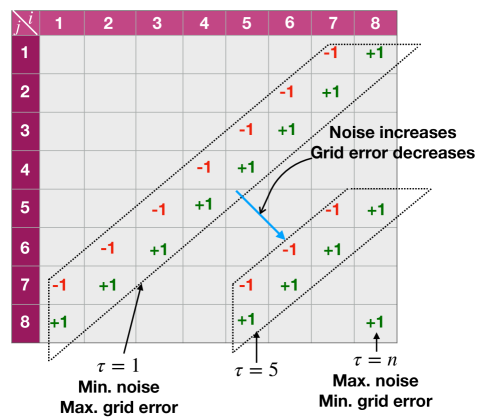
Figure 1: Schematic explaining the sparse grid combination technique and how the truncated combination can be used to minimize the total error. Here, $\tau=1$ corresponds to the standard sparse grid combination technique and $\tau=n$ corresponds to the regular grid. The indices $i$ and $j$ on the row and column headers indicate the mesh sizes of the component grids involved in the combination technique such that the $(i,j)$th component grid has mesh sizes $h_{i}=\frac{L}{2^{i}}$ and $h_{j}=\frac{L}{2^{j}}$, where $L$ is the length of the domain in each direction. The $+1$ and $-1$ are the combination coefficients $c_{i}$ in equation (2) corresponding to the component grids.

In Figure 1, we show for a 2D problem with a regular mesh of size $2^{8}\times 2^{8}$ the different combination strategies. The truncated combination technique [2, 3, 4] introduces a truncation parameter $\tau$, which is a positive integer that determines the component grids involved in the combination. If we consider a $2^{n}\times 2^{n}$ regular grid, then the value of $\tau=1$ corresponds to the standard combination technique in [28] and $\tau=n$ corresponds to the regular grid. By increasing $\tau$, fewer component grids are used in the combination technique, but each with finer mesh sizes than the previous $\tau$. This alleviates the issue of non-aligned and non-smooth functions by controlling the error term associated with the mixed fourth derivatives. Thus, the truncated combination technique provides a unified framework to transition from standard sparse grids to regular grid in terms of approximation capability by increasing $\tau$.

Let us consider a PIC simulation with $N_{p}$ total number of particles and $2^{n}\times 2^{n}$ regular grid with mesh size $h=\frac{L}{2^{n}}$. Now the regular grid with $\tau=n$ will have the least grid-based error and maximal noise because it has the mesh size $h$ in all the directions. The standard sparse grids technique with $\tau=1$ on the other extreme has maximal grid-based error and minimal noise as it has the mesh size $h$ in directions aligned with $x$ or $y$ axis but not in others. As we increase $\tau$ from $1$ to $n$ as shown in Figure 1, we decrease the grid-based error because of the inclusion of finer mesh sizes in the component grids but at the same time increase the particle noise due to decreased particles per cell or inclusion of higher wavenumbers in the filtering process (2). Thus depending on the smoothness and the orientation of the function there is an optimal $\tau$ at which the total error, which is the sum of grid-based error and particle noise, is minimized. In the following we will present a formal error analysis and propose a heuristic approach to estimate the optimal $\tau$.

4.3 Formal error analysis

In [1], a formal error analysis is shown for sparse PIC quantifying the grid-based error and particle noise. Since our codes are based on cell-centered grids (as it is the default choice in many plasma PIC codes [27, 17]), as mentioned in Proposition 1 the direct charge deposition in [1] and the current approach are not exactly equivalent because of the differences in the shape functions. Nevertheless, the order of accuracy is same for both the approaches and they differ only in constants. Hence, we will mostly follow the steps in [1] and generalize it to include the truncated combination technique.

As shown in [1] and appendix B, approximating $\rho_{e}$ in PIC simulations consists of two parts namely grid-based error and particle noise. In what follows we will quantify these two components and get an estimate of the total error.

4.3.1 Grid-based error

Let us remind that as per our notations, $\rho_{e}$ is the exact electron charge density given by

$$\rho_{e}({\bf x})=q_{e}\int f({\bf x},\mathbf{v})d\mathbf{v}=\int\int f({\bf\xi},\mathbf{v})\delta({\bf x}-{\bf\xi})d{\bf\xi}d\mathbf{v},$$

and $\varrho_{e}$ is the density on the regular grid after sparse grids transformation in equation (2). We will denote the grid error component of the total error as $||\rho_{e}-\varrho_{e}||_{grid}$, where for simplicity we have denoted the $L^{\infty}$ norm $||.||_{L^{\infty}}$ by $||.||$ (equivalently, we can also use the $L^{2}$-norm). In our approach the grid-based error comes from the approximation of delta-functions in the configuration space by shape functions of compact support as well as from the transfer operators $R$ and $P$.

Towards quantifying the grid-based error, for simplicity, let us consider a 2D PIC simulation in a periodic domain $[0,L]^{2}$ and a regular mesh of size $2^{n}\times 2^{n}$. Let the mesh size of the regular grid be $h_{n}=\frac{L}{2^{n}}$ and the mesh sizes of the component grids be $h_{i}=\frac{L}{2^{i}}$ and $h_{j}=\frac{L}{2^{j}}$ for the $(i,j)$th component grid in Figure 1. In our approach, we use the cloud-in-cell or linear interpolation operators for all the grid transfer operations. Hence, similar to [1, 28, 2], we assume an error expansion of the form $C_{1}(h_{i})h_{i}^{2}+C_{2}(h_{j})h_{j}^{2}+D_{1}(h_{i},h_{j})h_{i}^{2}h_{j}^{2}$ where $C_{1},C_{2},D_{1}$ are appropriate coefficient functions with a uniform upper bound. The summation over the component grids in equation (2) leads to pair-wise cancellations both in the standard sparse grid combination technique as well as in the truncated combination technique as shown in Figure 1. After multiplying with the combination coefficients and summing across all the component grids we get

$$(\rho_{e}-\varrho_{e})_{grid} =C_{1}(h_{n})h_{n}^{2}+C_{2}(h_{n})h_{n}^{2}$$

$$+\frac{4h_{n}^{2}L^{2}}{2^{2\tau}}\left[\frac{1}{4}\sum_{\begin{subarray}{c}i+j=n+\tau\\ i,j\geq\tau\end{subarray}}D_{1}(h_{i},h_{j})-\sum_{\begin{subarray}{c}i+j=n+\tau-1\\ i,j\geq\tau\end{subarray}}D_{1}(h_{i},h_{j})\right],$$ (4)

where we used the fact that $h_{i}h_{j}=\frac{h_{n}L}{2^{\tau}}$ when $i+j=n+\tau$ and $h_{i}h_{j}=\frac{h_{n}L}{2^{(\tau-1)}}$ when $i+j=n+\tau-1$. Taking the norm on both sides of the above equation and noting that there are $n-(\tau-1)$ component grids with $i+j=n+\tau$ and $(n-1)-(\tau-1)$ component grids with $i+j=n+\tau-1$ we get

$$||\rho_{e}-\varrho_{e}||_{grid} \leq\kappa_{1}h_{n}^{2}+\kappa_{2}h_{n}^{2}+\frac{4\beta_{1}h_{n}^{2}L^{2}}{2^{2\tau}}\left[\frac{n-(\tau-1)}{4}+\left\{(n-1)-(\tau-1)\right\}\right]$$

$$\leq h_{n}^{2}\left(\kappa_{1}+\kappa_{2}+\beta_{1}L^{2}2^{-2\tau}\left[5(n-\tau)+1\right]\right).$$ (5)

Here, $\kappa_{1},\kappa_{2}$ and $\beta_{1}$ are the constants corresponding to the upper bounds such that $||C_{1}(h_{n})||\leq\kappa_{1}$, $||C_{2}(h_{n})||\leq\kappa_{2}$ and $||D_{1}(h_{i},h_{j})||\leq\beta_{1}$, $\forall h_{i},h_{j}$. The same expression for the error is also obtained in [2] for the truncated combination in 2D. Similarly one can derive the estimates in 3D and the grid-based error in that case is given by

$$||\rho_{e}-\varrho_{e}||_{grid} \leq h_{n}^{2}\left(\kappa_{1}+\kappa_{2}+\kappa_{3}+(\beta_{1}+\beta_{2}+\beta_{3})L^{2}2^{-2\tau}\left[5(n-\tau)+1\right]\right.$$

$$+\left.\gamma L^{4}2^{-(4\tau+1)}\left\{25(n-\tau)^{2}-5(n-\tau)+2\right\}\right),$$ (6)

where the upper bounds for the coefficient functions in 3D are such that $||C_{d}(h_{n})||\leq\kappa_{d}$, $||D_{d}(h_{i},h_{j})||\leq\beta_{d}$ and $||F(h_{i},h_{j},h_{k})||\leq\gamma$ for $d=1,2,3$ and $\forall h_{i},h_{j},h_{k}$. By plugging in $\tau=1$ and $\tau=n$ in (5) and (6) we recover the estimates for the standard sparse grid combination in [28] and for regular grids respectively.

4.3.2 Particle noise

Now, we will consider the estimates for the particle noise in the total error. The particle noise is the result of approximating the expected value of the shape function by an arithmetic mean over a finite number of discrete particles. As per the error analysis in [1], in 2D the particle noise in each component grid is $\mathcal{O}\left(1/\sqrt{N_{p}h_{i}h_{j}}\right)$ and as stated in the grid error estimates we have $n-(\tau-1)$ component grids each with $h_{i}h_{j}=\frac{h_{n}L}{2^{\tau}}$ and $(n-1)-(\tau-1)$ component grids with $h_{i}h_{j}=\frac{h_{n}L}{2^{(\tau-1)}}$. Thus we can write an estimate for the particle noise as

$$||\rho_{e}-\varrho_{e}||_{noise} =\mathcal{O}\left(\sigma\left[\frac{n-(\tau-1)}{\sqrt{\frac{N_{p}h_{n}L}{2^{\tau}}}}+\frac{(n-1)-(\tau-1)}{\sqrt{\frac{N_{p}h_{n}L}{2^{(\tau-1)}}}}\right]\right)$$

$$=\mathcal{O}\left(\sigma\left\{\frac{2^{0.5(\tau-1)}\left[(n-\tau)(1+\sqrt{2})+\sqrt{2}\right]}{\sqrt{N_{p}h_{n}L}}\right\}\right),$$ (7)

where $\sigma$ is the particle noise constant. Following the same procedure, the noise estimate in 3D is given by

$$||\rho_{e}-\varrho_{e}||_{noise}=\mathcal{O}\left(\sigma\left\{\frac{2^{(\tau-2)}\left[(3+\sqrt{2})(n-\tau)^{2}+(5+\sqrt{2})(n-\tau)+4\right]}{\sqrt{N_{p}h_{n}L^{2}}}\right\}\right).$$ (8)

Again, by plugging in $\tau=1$ and $\tau=n$ in equations (7), (8) we recover the estimates shown in [1] for standard sparse grids technique and regular grids respectively. With the grid and particle error estimates in hand we will show how these can be used in practice to adaptively select the optimal $\tau$.

4.3.3 A heuristic approach for estimating coefficients of the error

In order to use the grid and particle error estimates derived in the previous section we need to have an estimate of the coefficients. To that extent, we note that a rigorous derivation of coefficients for the current approach in case of cell-centered grids depends on the ratio of the mesh sizes of the component grids to the regular grid and is more involved. Instead in this section we approximate the grid and particle coefficients based on heuristic arguments and empirical observations and intend to improve these choices in the future iterations of our algorithm. Let us first consider the grid-based error before we discuss the particle noise. As explained in [1, 34] and equations (32) and (33) in appendix B, the coefficient functions in the grid error estimates are proportional to the derivatives of the charge density $\rho_{e}$ such that

$$C_{1}\propto\frac{\partial^{2}\rho_{e}}{\partial x^{2}},C_{2}\propto\frac{\partial^{2}\rho_{e}}{\partial y^{2}},C_{3}\propto\frac{\partial^{2}\rho_{e}}{\partial z^{2}},D_{1}\propto\frac{\partial^{4}\rho_{e}}{\partial x^{2}\partial y^{2}}$$

$$D_{2}\propto\frac{\partial^{4}\rho_{e}}{\partial y^{2}\partial z^{2}},D_{3}\propto\frac{\partial^{4}\rho_{e}}{\partial z^{2}\partial x^{2}},F\propto\frac{\partial^{6}\rho_{e}}{\partial x^{2}\partial y^{2}\partial z^{2}}.$$

In PIC we only have an approximation of $\rho_{e}$ on the regular grid, which we call $\tilde{\rho}_{e}$ as defined in equation (34), and this also contains the particle noise. In order to have a realistic approximation of the derivatives of the charge density from noisy regular PIC data $\tilde{\rho}_{e}$ we perform a denoising by thresholding in the Fourier domain. Specifically, we first take the Fourier transform of the density on the regular grid $\hat{\rho}_{e}=\mathcal{F}\left(\tilde{\rho}_{e}\right)$ and perform a hard thresholding such that

$$\hat{\rho}_{e}=\begin{cases}\hat{\rho}_{e}&\quad|\hat{\rho}_{e}|\geq\epsilon,\\ 0&\quad|\hat{\rho}_{e}|<\epsilon,\end{cases}$$ (9)

where $\epsilon$ is the threshold for denoising and $|\hat{\rho}_{e}|$ denotes the magnitude of the Fourier transform $\hat{\rho}_{e}$. This type of denoising is common in signal processing as well as wavelet denoising [35] techniques.

The threshold parameter $\epsilon$ is a function of the number of particles per cell $P_{c}$, the initial sampling method and also the distribution $f$. It determines how much noise and signal is removed by the denoising process. Too low a value will not remove much noise and too high a value may remove a significant portion of the signal along with the noise. However, in contrast to denoising techniques in signal processing where after applying this threshold one performs an inverse transform to get the signal in the physical domain, we emphasize the fact that for our scheme we only use it for selecting the truncation parameter $\tau$ (which performs the final filtering). Hence the threshold $\epsilon$ does not need to be optimal, and we only need to ensure that we do not pick up excessive noise.

At present, we use an ad-hoc strategy to select the value of $\epsilon$ as a certain percentage of the maximum value of $|\hat{\rho}_{e}|$, namely $\epsilon=\alpha\max\left(|\hat{\rho}_{e}|\right)$, where $\alpha$ denotes the percentage. To determine $\alpha$ in our algorithm, for a certain number of particles per cell $(P_{c})_{ref}$ (e.g., 5) we run the PIC simulation for a few different values of $\alpha$ and pick the minimum value necessary for denoising. To reduce the run time we use a coarse mesh necessary for the problem in these simulations. Once we pick the value of $\alpha$ for a reference number of particles per cell $(P_{c})_{ref}$, we run simulations with other values of $P_{c}$ by multiplying $\alpha$ by $\sqrt{(P_{c})_{ref}/P_{c}}$, as we know the noise in PIC methods scales as $1/\sqrt{P_{c}}$. In the numerical results in section 5, we performed the experiments with few different $\alpha$ to examine robustness. It is observed that within a range of $\alpha$ (which is problem specific) the results not change much. In our future work we will develop a more systematic way to pick the threshold from the density data, based on techniques similar to the ones used in wavelet denoising [35]. Machine learning techniques can also be used for this purpose and this is another direction we will pursue.

After denoising the charge density, we compute the derivatives in the Fourier domain and perform inverse transforms. Next, in order to fix the constants in front of these derivatives in appendix B we derive the grid-based error for regular PIC schemes. Since, each component grid in the sparse grid combination technique is a regular grid with mesh sizes $h_{i}$, $h_{j}$ and $h_{k}$, equations (32) and (33) can be used for determining the constants involved in the upper bounds. To that extent, we note that by means of the grid transfer operations with $R$ and $P$ we incur two times the grid-based error of similar magnitude given in equations (32) and (33). Moreover, the charge density $\tilde{\rho}_{e}$ in the regular grid adds another $1/12$ in front of the second derivative terms. Summing all these contributions we get an estimate for the coefficients in equations (5) and (6) as

$$\kappa_{1}=\frac{1}{4}\left\|\frac{\partial^{2}\bar{\rho}_{e}}{\partial x^{2}}\right\|,\kappa_{2}=\frac{1}{4}\left\|\frac{\partial^{2}\bar{\rho}_{e}}{\partial y^{2}}\right\|,\kappa_{3}=\frac{1}{4}\left\|\frac{\partial^{2}\bar{\rho}_{e}}{\partial z^{2}}\right\|,\beta_{1}=\frac{1}{72}\left\|\frac{\partial^{4}\bar{\rho}_{e}}{\partial x^{2}\partial y^{2}}\right\|$$

$$\beta_{2}=\frac{1}{72}\left\|\frac{\partial^{4}\bar{\rho}_{e}}{\partial y^{2}\partial z^{2}}\right\|,\beta_{3}=\frac{1}{72}\left\|\frac{\partial^{4}\bar{\rho}_{e}}{\partial z^{2}\partial x^{2}}\right\|,\gamma=\frac{1}{864}\left\|\frac{\partial^{6}\bar{\rho}_{e}}{\partial x^{2}\partial y^{2}\partial z^{2}}\right\|,$$ (10)

where $\bar{\rho}_{e}$ is the denoised charge density defined in equation (24).

Finally, following the particle noise estimates in equations (48) and (49) as well as [1, 16], for our algorithm we take

$$\sigma=\sqrt{\left(2/3\right)^{d}\left\|Q_{e}\tilde{\rho}_{e}\right\|}$$ (11)

in equations (7) and (8), where $d$ is the dimension and $\tilde{\rho}_{e}$ is the charge density on the regular grid before denoising as defined in equation (34). Here, we use the density $\tilde{\rho}_{e}$ instead of the denoised density $\bar{\rho}_{e}$ as it helps in adjusting the particle constant with respect to different sampling techniques.

Through numerical experiments we also found another choice for the coefficients in the grid-based error and particle noise as

$$\kappa_{1}=\left\|k_{x}^{2}\hat{\rho}_{e}\right\|,\kappa_{2}=\left\|k_{y}^{2}\hat{\rho}_{e}\right\|,\kappa_{3}=\left\|k_{z}^{2}\hat{\rho}_{e}\right\|,\beta_{1}=\left\|k_{x}^{2}k_{y}^{2}\hat{\rho}_{e}\right\|$$

$$\beta_{2}=\left\|k_{y}^{2}k_{z}^{2}\hat{\rho}_{e}\right\|,\beta_{3}=\left\|k_{x}^{2}k_{z}^{2}\hat{\rho}_{e}\right\|,\gamma=\left\|k_{x}^{2}k_{y}^{2}k_{z}^{2}\hat{\rho}_{e}\right\|,\sigma=\sqrt{\left\|Q_{e}\tilde{\rho}_{e}\right\|}$$ (12)

where $k_{x},k_{y}$ and $k_{z}$ are the wavenumbers in $x,y$ and $z$ respectively. We do not present detailed results, but for the numerical experiments in section 5 as well as for other synthetic examples in the context of interpolation we found this choice yields similar optimal $\tau$ values as that of the constants in equations (10) and (11). It has an added advantage that we do not need to take inverse transform of the derivatives, which is three in 2D and seven in 3D. Thus it may be of interest from a practical point of view, and for the numerical experiments in section 5 we observed up to 7 times speedup in the $\tau$ estimation part with this choice compared to the ones in equations (10) and (11).

In Algorithm 1 we consolidate the steps in the optimal $\tau$ estimator algorithm. For the range of $\tau$, we consider $[1,n-3]$ for 2D and $[1,n-2]$ for 3D where $2^{n}$ is the number of points in the regular grid in each dimension. This is because in 2D, the total number of degrees of freedom in $\tau=n-2$ sparse grid is same as that of the regular grid and $\tau=n-1$ has more degrees of freedom than the regular grid. Thus we include up to $n-3$ in 2D to have a higher value of $P_{c}$ than for the regular grid and hence less particle noise. In 3D on the other hand the permissible range of $\tau$ is $[1,n-2]$ and even with $\tau=n-2$ we have fewer degrees of freedom than for the regular grid.

4.4 Implementation in a HPC PIC code base.

Once the optimal $\tau$ is obtained from Algorithm 1 we need to perform sparse grids noise reduction. In Algorithm 2 we present a matrix-free implementation of the sparse grids filtering in equation (2). This implementation would be suitable for large-scale high performance PIC code bases like OPAL. In these codes the density in the regular grid is domain decomposed between different processors and in Algorithm 2 each processor holds the entire component grid in the combination technique. For moderate values of $\tau$, each component grid has very few degrees of freedom compared to the regular grid and this is not very expensive in terms of memory. However for high $\tau$, the component grids involved in the combination has a considerable number of degrees of freedom (especially in 3D) and hence both memory as well as the MPI_Allreduce step in Algorithm 2 could present a bottleneck. In our future work we will also split up the component grids between processors which would require a more complicated parallelization strategy as shown in [36].

If the parallelization of the code base uses MPI for inter-node parallelism and OpenMP for intra-node parallelism then the for loop over component grids in Algorithm 2 can be done in parallel with OpenMP. Algorithms 1 and 2 would go in between steps 1 and 2 in the regular PIC procedure outlined in section 2. Ingredients such as FFT which are required for the tauEstimator algorithm are already available in many of the large-scale PIC code bases and hence these two algorithms can be incorporated inside them very easily without any modification to the other parts.

1:  Compute Fourier transform of the charge density $\hat{\rho}_{e}=\mathcal{F}\left(\tilde{\rho}_{e}\right)$.

2:  Perform denoising by hard thresholding according to equation (9).

3:  Compute the constants for the grid-based error with (10) and the particle error constant (11).

4:  for $\tau=1$ to $n-3$ for 2D and $n-2$ for 3D do

5:     Evaluate grid-based error and particle noise using equations (5),(7) for 2D and (6),(8) for 3D.

6:  end for

7:  Select the $\tau$ with minimum total error.

Algorithm 1 tauEstimator: An algorithm for estimating optimal $\tau$.

1:  for $i=1$ to $nc$ do

2:     Each processor deposits their regular grid partition of $\tilde{\rho}_{e}$ to the $i$th component grid using the transfer operator $R_{i}$ in equation (3).

3:     MPI_Allreduce to add contributions from all processors on the $i$th component grid.

4:     Each processor interpolates from the $i$th component grid to their regular grid partition of $\tilde{\rho}_{e}$ using transfer operator $P_{i}$ in equation (3).

5:     Multiply by combination coefficient and accumulate.

6:  end for

Algorithm 2 transferToSparse: An algorithm for sparse grids based noise reduction with a given $\tau$.

Remark 1.

In general the charge density $\varrho_{e}$ after sparse grids transformation is not guaranteed to be positive everywhere. This is not unique to our approach and also happens in other noise reduction strategies such as high-order shape functions [20], compensating filters [6] and wavelet-based density estimation [37]. In our numerical results in section 5 we do not observe any problems caused by this. However, we could adopt the density redistribution procedure used in [20] to make the charge density positive everywhere after the sparse grids transformation. This will be studied in future versions of the algorithm. Also, as shown in [26], the filtering procedures used in explicit PIC simulations improve energy conservation but at the loss of momentum conservation. In our future study we will investigate in detail the impact of the noise reduction strategy on energy and momentum conservation and report the results.

5 Numerical results

In this section we will test the performance of the adaptive noise reduction strategy on two benchmark problems in plasma physics and beam dynamics; namely two-dimensional diocotron instability, and three-dimensional electron dynamics in a Penning trap with a neutralizing ion background. These test cases produce fine-scale structures during the nonlinear evolution and thus can be used to evaluate the ability of the adaptive $\tau$ method to capture them while still reducing noise. Also, they are very relevant to the large-scale accelerator simulations which we intend to perform in our future works.

In all the simulations we consider a periodic box $\Omega=[0,L]^{d}$, where $d$ is the dimension and $L$ is the length in each dimension. The charge to mass ratio $q_{e}/m_{e}$ in all our simulations is $-1$. In measuring the error in field quantities we use the relative discrete $L^{2}$-norm also known as the normalized root mean squared error given by

$$\mathcal{E}(\boldsymbol{\psi})=\sqrt{\frac{\sum_{i=1}^{N_{points}}\left(\boldsymbol{\psi}({\bf x}_{i})-\boldsymbol{\psi}_{ref}({\bf x}_{i})\right)^{2}}{\sum_{i=1}^{N_{points}}(\boldsymbol{\psi}_{ref}({\bf x}_{i}))^{2}}},$$ (13)

where $\boldsymbol{\psi}$ is any field quantity, $\boldsymbol{\psi}_{ref}$ is the reference field which is obtained from an ensemble average of high-resolution regular PIC simulations and ${\bf x}_{i}$ are the locations of points in the domain at which we measure the error. This error is for a particular time instant and we measure the error at few instants in the whole simulation. In both numerical examples, we calculate the error for regular PIC, adaptive $\tau$ PIC and fixed $\tau$ PIC with the range of $\tau$ taken to be the same as the one used in the tauEstimator Algorithm 1. By means of these error curves we can see how well the adaptive $\tau$ algorithm performs in terms of picking the optimal $\tau$ and also how the errors compare to that of the regular PIC results with different number of particles per cell $P_{c}$. We always define the number of particles per cell $P_{c}$ based on the regular grid. It is given by

$$P_{c}=\frac{N_{p}}{N_{c}}=\frac{N_{p}}{2^{nd}}.$$

For the time integration we use the leap frog method and for the Poisson equation we use the second order cell-centered finite difference method as in [38, 39] with single level and without any spatial adaptivity. For solving the linear system arising from the discretized Poisson equation we use the smoothed aggregation algebraic multigrid (SAAMG) from the second generation Trilinos MueLu library [40]. The stopping tolerance for the iterative solver is set as $10^{-10}$ multiplied by the infinity norm of the right hand side. More details on the solver can be found in [39]. The code is written on top of a C++ miniapp based on the particle accelerator library OPAL [27] and box structured adaptive mesh refinement library AMReX [41]. Even though FFT solver would be the most accurate and fastest option [42] in this context, the reason for the above choice of field solver is in our future work we want to extend the current approach to include adaptive mesh refinement. Also, the conclusions of the present study will not be much affected by this choice and will be applicable for FFT solver too.

All the computations are performed on the Merlin6 HPC cluster at the Paul Scherrer Institut, the details of which are as follows. Each Merlin6 node consists of 2 sockets and each socket in turn has Intel Xeon Gold 6152 processor with $22$ cores at 2.1-3.7GHz. There are 2 threads in each core, however in all the present computations we only use single thread. Each node contains 384 GB DDR4 memory in total.

5.1 2D diocotron instability

As a first example, we consider the 2D diocotron instability test case as already described in [1]. In this test case, we have electrons with a hollow density profile immersed in a neutralizing immobile and uniform ion background and confined by a uniform external axial magnetic field. The magnetic field is strong enough that the electron dynamics is dominated by advection in the self-consistent $\mathbf{E}_{sc}\times\mathbf{B}_{ext}$ velocity field [43, 44, 45, 46]. The initial electron density profile is not monotonic in the radial direction, which translates to an $\mathbf{E}_{sc}\times\mathbf{B}_{ext}$ shear flow which is unstable to what is known as the Kelvin-Helmholtz shear layer instability [43, 47, 46] in fluid dynamics, and the diocotron instability in beam and plasma physics [11, 48, 43]. This instability deforms the initially axisymmetric electron density distribution, leading, in the nonlinear phase, to the formation of a discrete number of vortices, and eventually breakup [46, 48]. This test case has importance both from a fundamental physics point of view [11, 48, 43] as well as in practical applications such as beam collimation [49].

The parameters for this test case are as follows and are very similar to the ones in [1]. We apply a uniform external magnetic field $\mathbf{B}_{ext}=\left\{0,0,5\right\}$ along the $z-$axis in a domain of length $L=22$. The external electric field $\mathbf{E}_{ext}={\bf 0}$ for this problem. The initial distribution is given by

$$f(t=0) =\frac{C}{2\pi}e^{-|\mathbf{v}|^{2}/2}\exp\left\{-\frac{(r-L/4)^{2}}{2(0.03L)^{2}}\right\},$$

$$r =\sqrt{(x-L/2)^{2}+(y-L/2)^{2}},$$ (14)

and the constant $C$ is chosen such that the total electron charge $Q_{e}=-400$. We sample the phase space using Gaussian distribution in the velocity variables with mean $0$ and standard deviation $1$. For the configuration space, we use a uniform distribution for $\theta$ in $[0,2\pi]$, and for $r$ a Gaussian distribution with mean $L/4$ and standard deviation $0.03L$. From $(r,\theta)$ we do the polar to Cartesian transformation to get $(x,y)$ for the particles. We will refer this sampling as Gaussian sampling to differentiate it from the uniform sampling which will be presented later in this section.

For denoising in equation (9), we take $\epsilon=\alpha\sqrt{(P_{c})_{ref}/P_{c}}\max(|\hat{\rho}_{e}|)$ as explained in section 4.3.3, where $(P_{c})_{ref}=5$ and $\alpha=0.01$. This means that with $5$ particles per cell, charge densities with Fourier amplitude less than 1 percent of the maximum amplitude will be set to 0 and for other $P_{c}$ the threshold will be scaled accordingly. The time step of the time integrator is chosen as $\Delta t=0.02$ and the simulation is run till final time $T=17.5$.

(a) time=0

(b) time=10

(c) time=17.5

(d) time=0

(e) time=10

(f) time=17.5

(g) time=0

(h) time=10

(i) time=17.5

(j) time=0

(k) time=10

(l) time=17.5

Figure 2: 2D diocotron instability. Gaussian sampling: Evolution of the electron charge density with time for regular PIC, $P_{c}=5$ (first row); $\tau=1$, $P_{c}=5$ (second row); adaptive $\tau$, $P_{c}=5$ (third row); and regular PIC, $P_{c}=80$ (fourth row). The mesh considered here is $1024^{2}$.

Figure 2 shows the evolution of the electron charge density with time for regular, $\tau=1$ and adaptive $\tau$ PIC for a $1024^{2}$ mesh. For the first three rows $P_{c}=5$ and for the last row $P_{c}=80$. From the first and second rows we can see that while the regular PIC results are dominated by noise, $\tau=1$ results are dominated by grid error due to the smearing of fine scale structures. This is also noted in [1] in their sparse PIC studies. In contrast, the adaptive $\tau$ results in the third row strikes a balance between the grid-based error and noise and are in close agreement (in visual norm) with the regular PIC results with high $P_{c}$ in the fourth row.

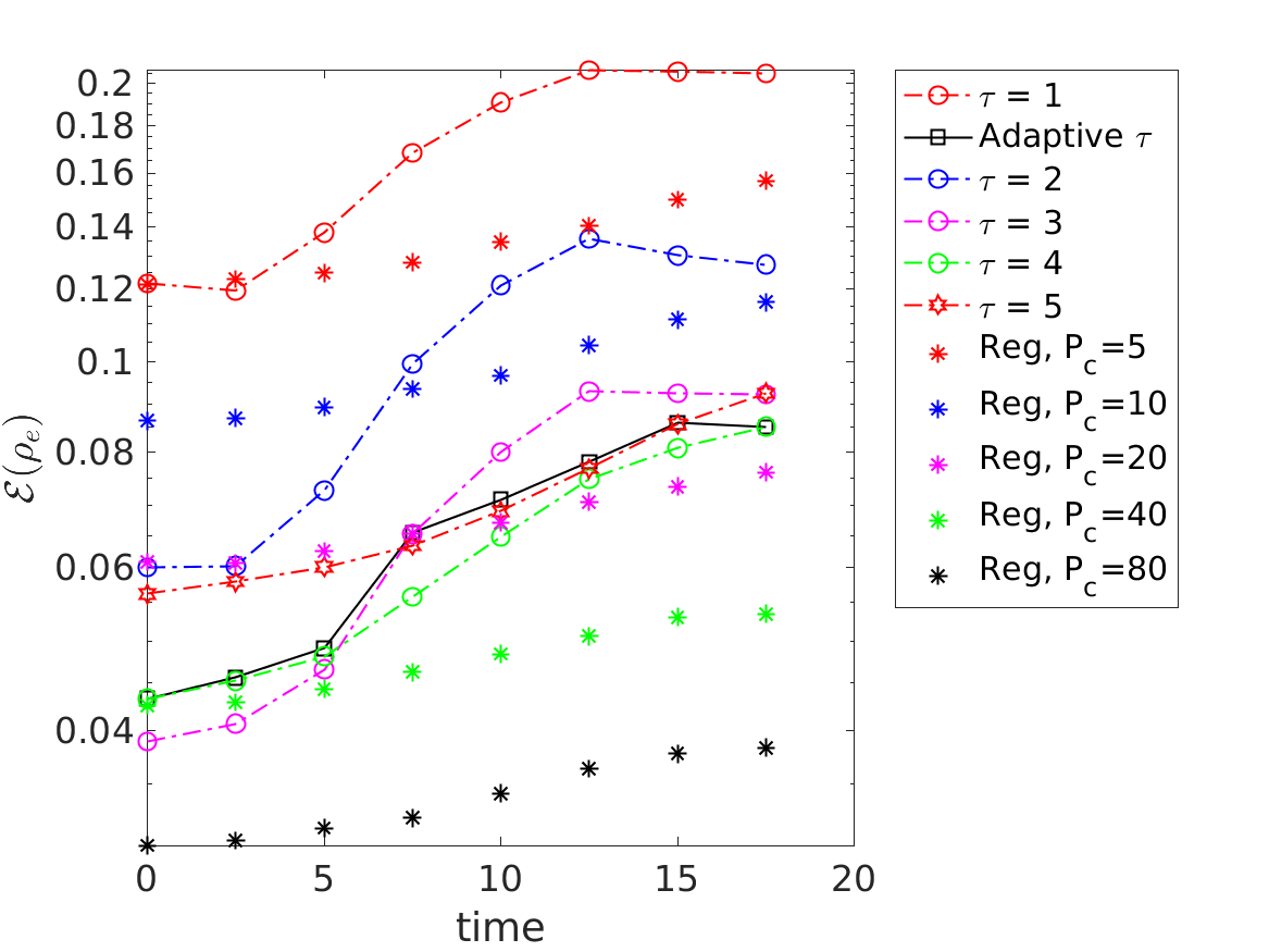
(a) $256^{2}$, $P_{c}=5$

(b) $256^{2}$, $P_{c}=5$

(c) $512^{2}$, $P_{c}=5$

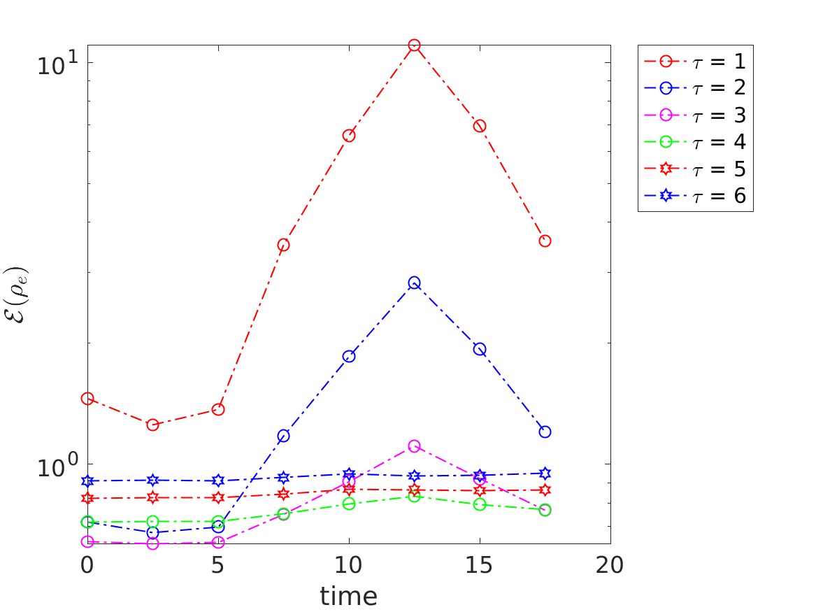
(d) $512^{2}$, $P_{c}=5$

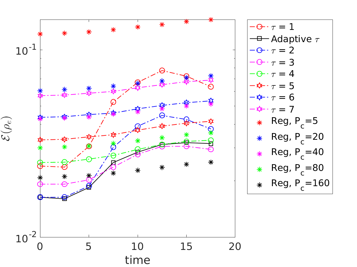
(e) $1024^{2}$, $P_{c}=5$

(f) $1024^{2}$, $P_{c}=5$

Figure 3: 2D diocotron instability. Gaussian sampling: Electron charge density error comparison between regular (Reg), fixed $\tau$ and adaptive $\tau$ PIC. The left column is the actual error calculated using equation (13) and the right column is the estimations from the $\tau$ estimator based on which the optimal $\tau$ is selected. The fixed as well as adaptive $\tau$ has the number of particles per cell $P_{c}=5$.

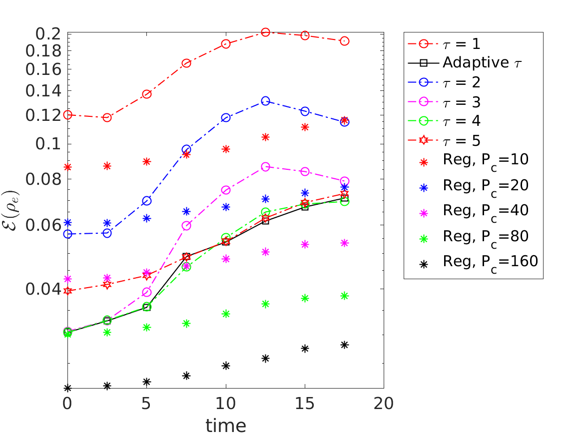
(a) $256^{2}$, $P_{c}=10$

(b) $256^{2}$, $P_{c}=10$

(c) $512^{2}$, $P_{c}=10$

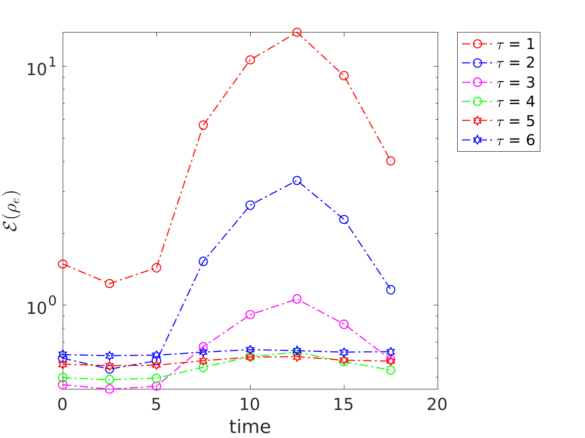
(d) $512^{2}$, $P_{c}=10$

(e) $1024^{2}$, $P_{c}=10$

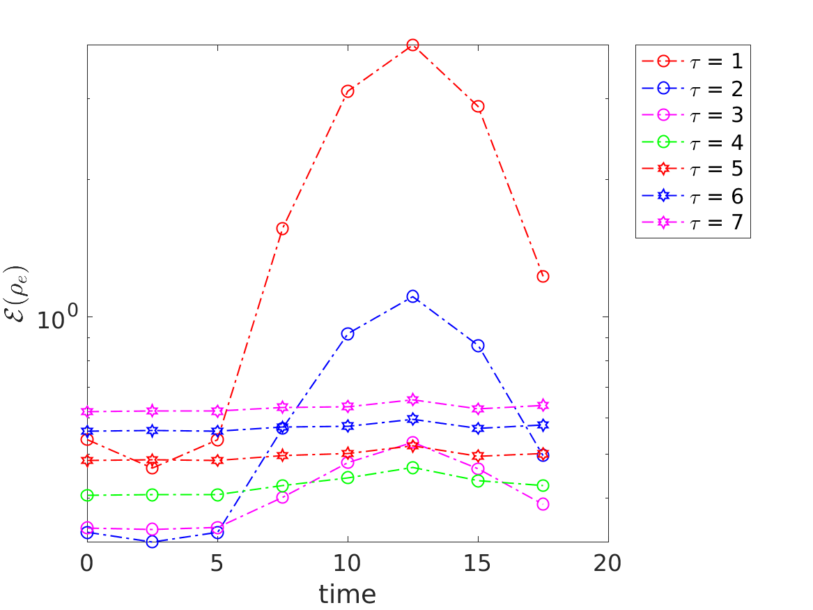
(f) $1024^{2}$, $P_{c}=10$

Figure 4: 2D diocotron instability. Gaussian sampling: Electron charge density error comparison between regular (Reg), fixed $\tau$ and adaptive $\tau$ PIC. The left column is the actual error calculated using equation (13) and the right column is the estimations from the $\tau$ estimator based on which the optimal $\tau$ is selected. The fixed as well as adaptive $\tau$ has the number of particles per cell $P_{c}=10$.

(a) $256^{2}$, $P_{c}=20$

(b) $256^{2}$, $P_{c}=20$

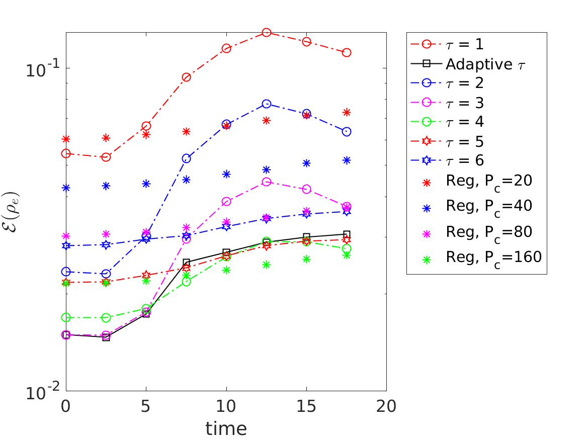
(c) $512^{2}$, $P_{c}=20$

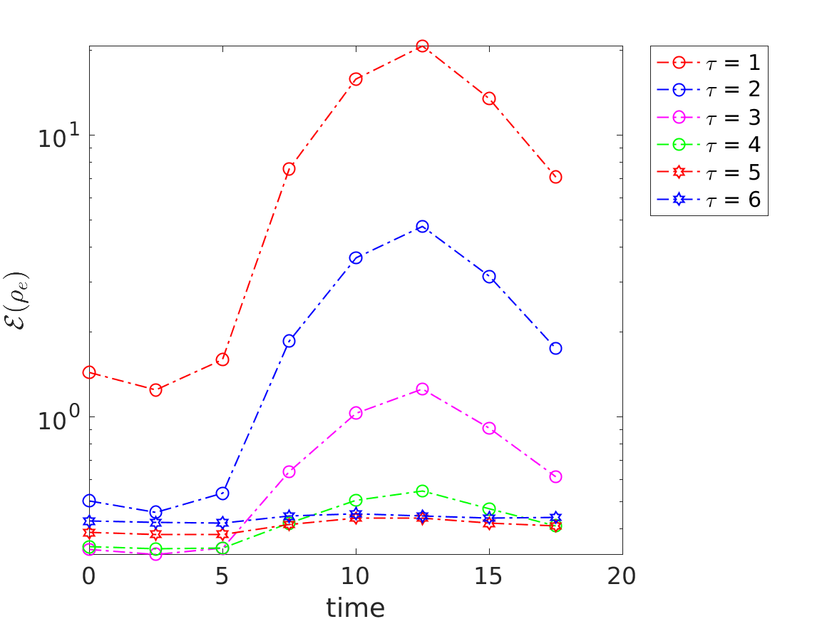
(d) $512^{2}$, $P_{c}=20$

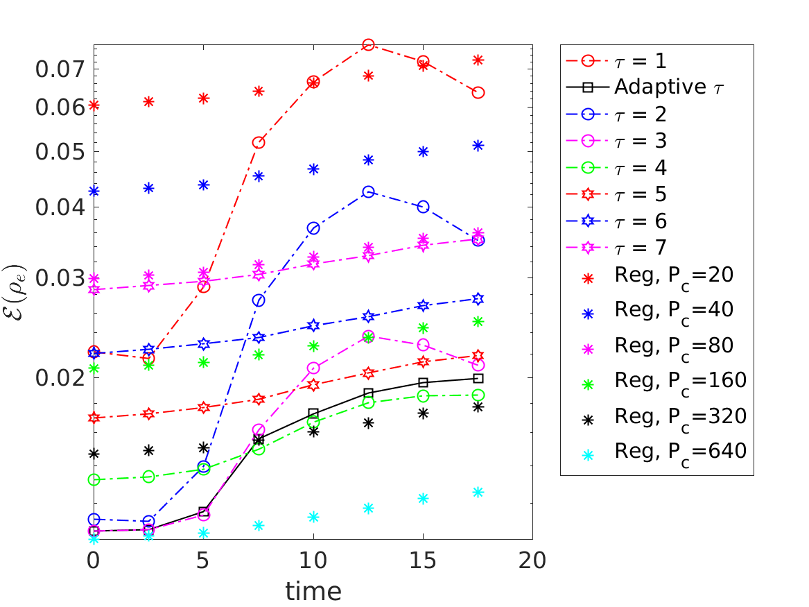
(e) $1024^{2}$, $P_{c}=20$

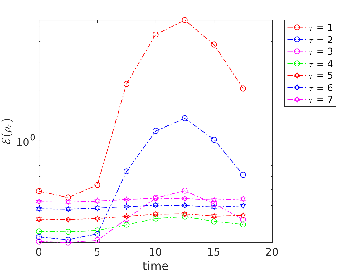
(f) $1024^{2}$, $P_{c}=20$

Figure 5: 2D diocotron instability. Gaussian sampling: Electron charge density error comparison between regular (Reg), fixed $\tau$ and adaptive $\tau$ PIC. The left column is the actual error calculated using equation (13) and the right column is the estimations from the $\tau$ estimator based on which the optimal $\tau$ is selected. The fixed as well as adaptive $\tau$ has the number of particles per cell $P_{c}=20$. The errors for regular PIC with $P_{c}=320$ and $640$ are calculated from that of $P_{c}=160$ based on the theoretical particle error scaling $1/\sqrt{Pc}$. This is based on the observation that the errors for the regular PIC are in the noise dominated regime.

In order to make a quantitative comparison, in the left columns of Figures 3-5, the error in $\rho_{e}$ calculated using (13) at 8 time instants is shown for three different meshes $256^{2},512^{2},1024^{2}$ and number of particles per cell $P_{c}=5,10,20$. For regular PIC we also carried out simulations at higher $P_{c}$, namely $40,80,160$ in order to compare the accuracy level with adaptive $\tau$ results. The reference in equation (13) is computed using the average of 8 independent regular PIC simulations each with a $1024^{2}$ mesh and $P_{c}=320$. In equation (13), the $N_{points}$ are taken as the cell-centered points in the mesh under consideration and the reference $\rho_{e}$ is interpolated to these points for calculating error. In Figure 5(e), for calculating the error with regular PIC at $P_{c}=320,640$ we divided the error for $P_{c}=160$ by $\sqrt{2}$ and $\sqrt{4}$ respectively as we observed the errors are already in the noise dominated regime and follow the scaling $1/\sqrt{P_{c}}$. On the right columns of Figures 3-5 are the estimations of the error for different $\tau$ values from the $\tau$ estimator divided by the root mean squared value of the reference $\rho_{e}$. It is based on these curves that the optimal $\tau$, i.e. the one with minimum error, is selected at each time step during the simulation.

From the left columns of Figures 3-5, we can see that in general the adaptive $\tau$ performs well in terms of picking one of the $\tau$ values with the lowest error (if not the optimal $\tau$ at all time instants). The shapes of the error curves for individual $\tau$ values are also similar for the estimated and actual ones. It demonstrates the ability of our estimator to predict correct error dynamics for different $\tau$ cases. While we do not have to worry about the magnitude of the errors in the estimator, the ordering of the error curves between different $\tau$ values is of importance as it decides the optimal $\tau$, and we want it to be close to the actual scenario on the left columns. To that extent, we make an observation that in the time interval $t\in[7.5,17.5]$ the difference in the magnitude of errors between different $\tau$ values in the estimator differs more from the actual scenario than in the time interval $t\in[0,7.5)$. More specifically, for low $\tau$ values ($\tau=1,2,3$) the estimator predicts a significantly higher error compared to the other $\tau$ values in that regime.

One of the reasons for this behavior is for low $\tau$ cases e.g., $\tau=1,2$ and $3$, the number of component grids in the combination technique is higher than that for the high $\tau$ cases. Since we use the triangle inequality to bound the errors, both the grid and particle errors tend to be more over-estimated for the low $\tau$ cases than those for the high $\tau$ ones. Another reason is, in the estimates for the grid error we use the derivatives based on the regular grid. While this is a sharper upper bound for high $\tau$, the derivatives seen in reality by the low $\tau$ cases for functions with fine scale structures will be smaller because of the larger mesh sizes. Indeed, fine scale structures form in the time interval $t\in[7.5,17.5]$ and hence grid error dominated for the simulations with sparse grids noise reduction.

In spite of these differences, in all the cases even with the predicted sub-optimal $\tau$ the error values of the adaptive $\tau$ PIC is significantly lower than that of the regular PIC with same $P_{c}$. If we use some problem specific information, then it may be possible to reduce the over-estimations in the grid and particle errors by introducing a correction factor for different $\tau$ values.

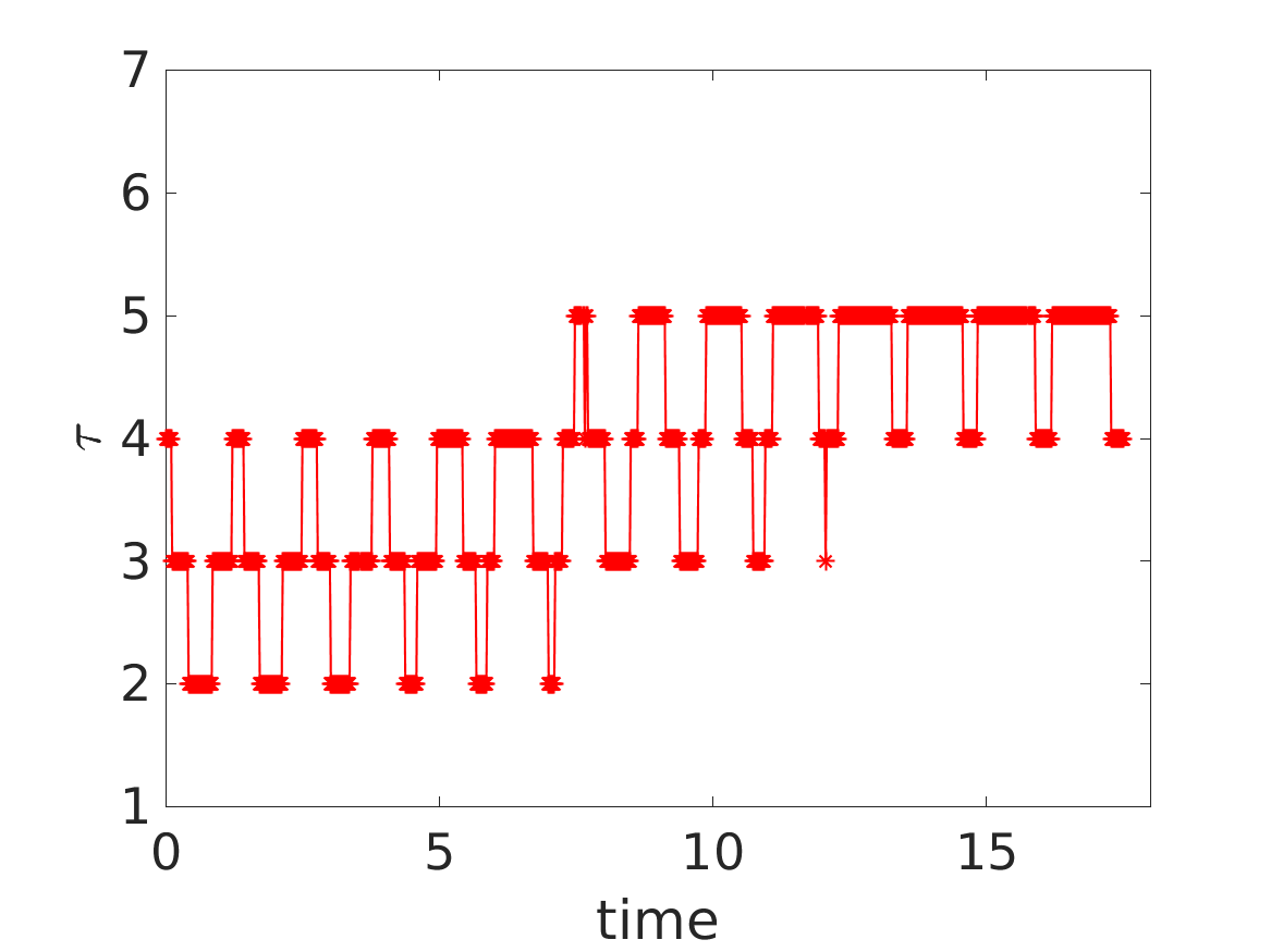
(a) $256^{2}$, $P_{c}=5$

(b) $512^{2}$, $P_{c}=5$

(c) $1024^{2}$, $P_{c}=5$

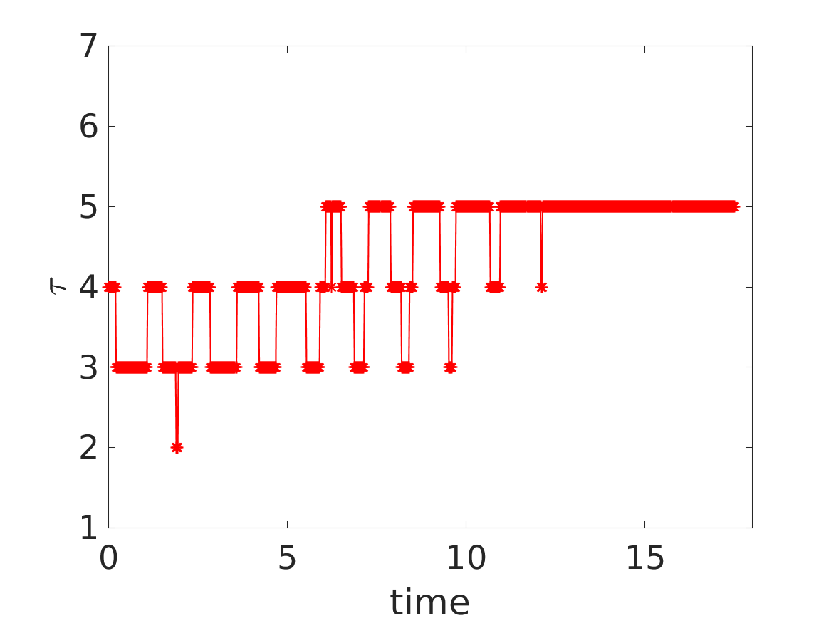
(d) $256^{2}$, $P_{c}=10$

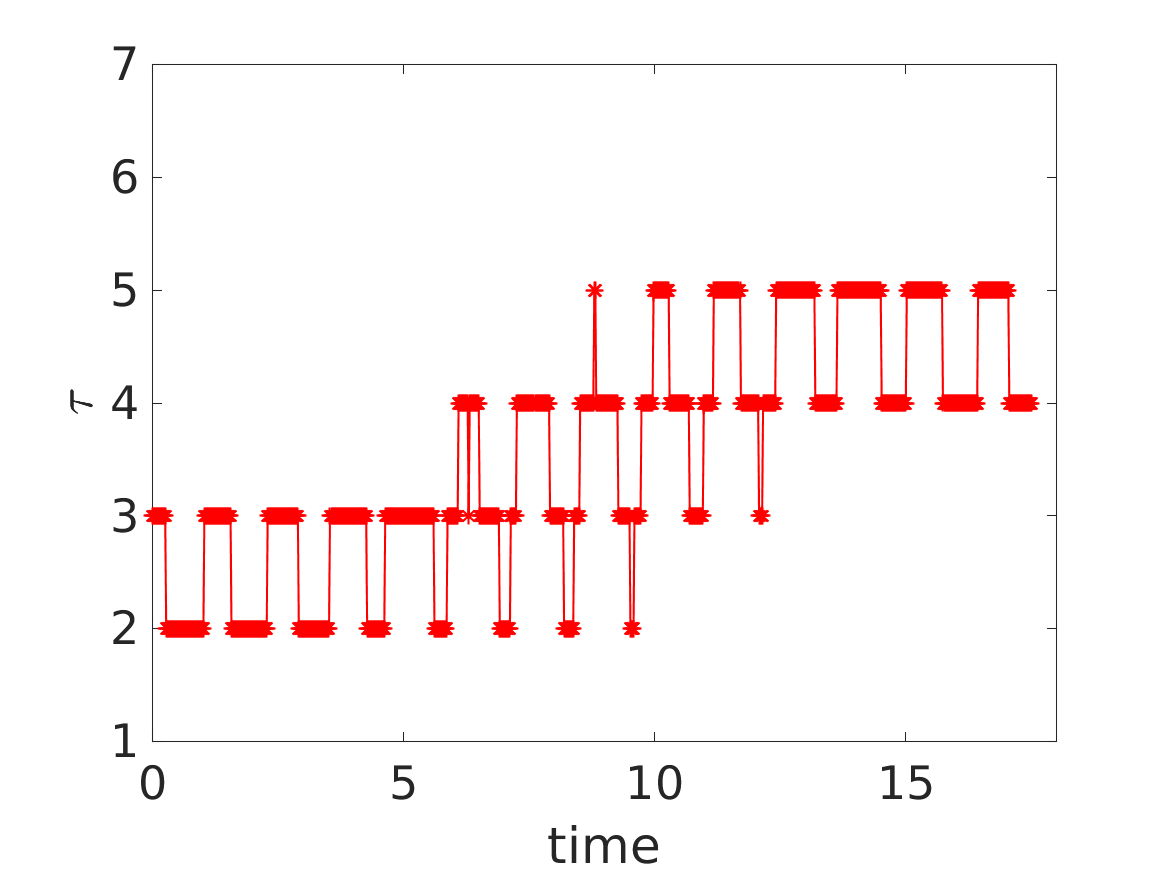
(e) $512^{2}$, $P_{c}=10$

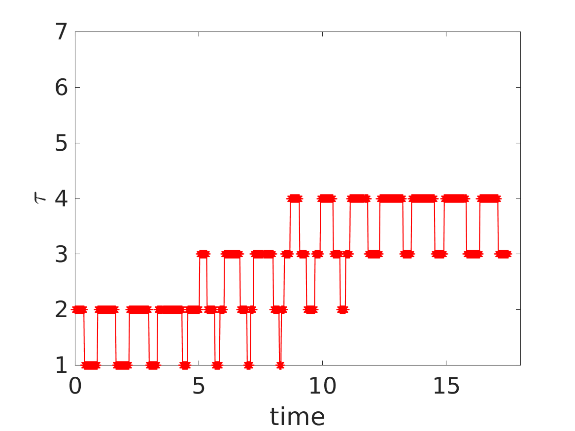
(f) $1024^{2}$, $P_{c}=10$

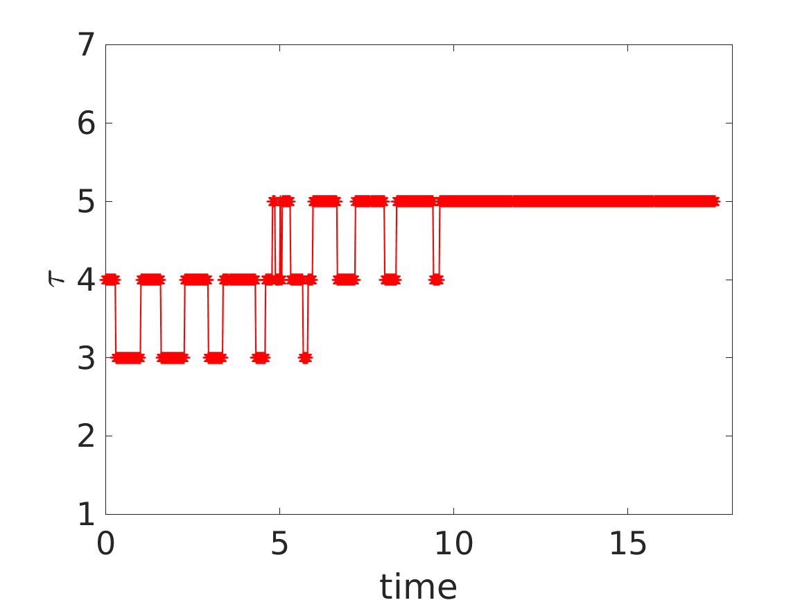
(g) $256^{2}$, $P_{c}=20$

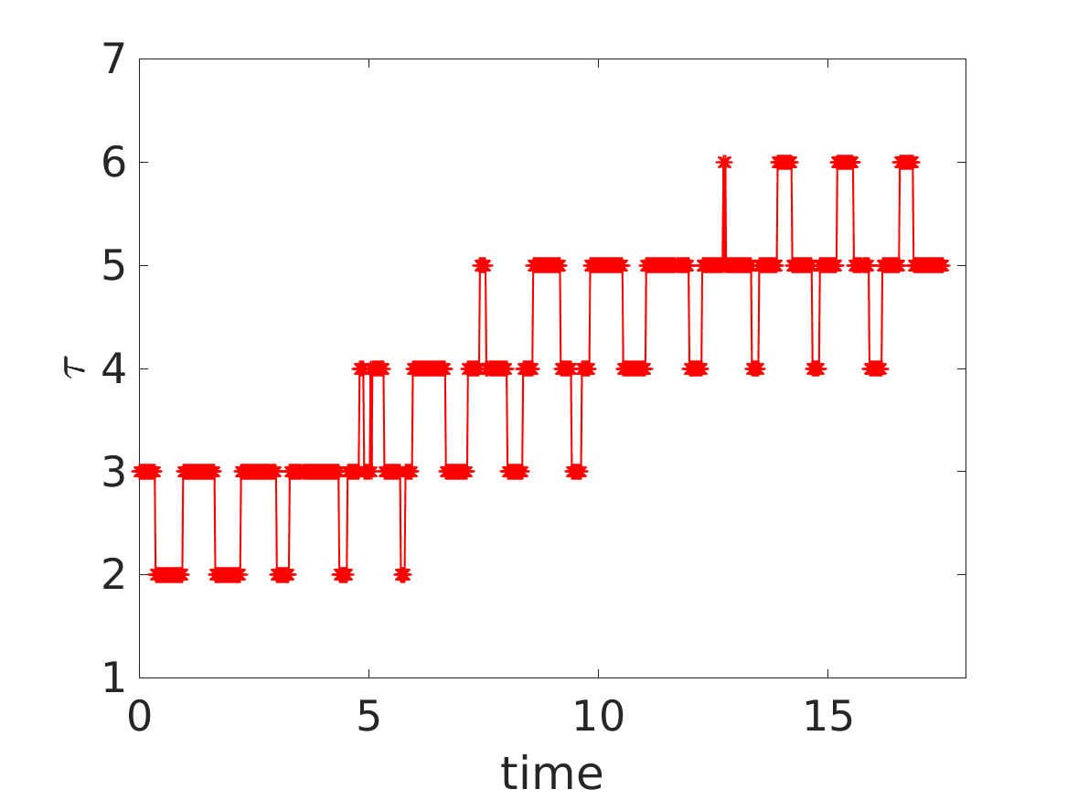
(h) $512^{2}$, $P_{c}=20$

(i) $1024^{2}$, $P_{c}=20$

Figure 6: 2D diocotron instability. Gaussian sampling: Time history of $\tau$ for different mesh sizes and number of particles per cell $P_{c}$.

In Figure 6, the time history of $\tau$ is shown for the meshes and $P_{c}$ considered in Figures 3-5. Here we can see that for the same $P_{c}$, when we decrease the mesh size, i.e., going from left to right in Figure 6, the $\tau$ values decrease. This is because we are moving from the grid error dominated regime to the particle error dominated regime. On the other hand, for the same mesh size and increasing $P_{c}$, i.e., moving from top to bottom in Figure 6, the $\tau$ values increase as we are moving from the particle error dominated regime to the grid error dominated regime. Also, for a particular mesh size and given $P_{c}$ the later time instants have higher $\tau$ compared to the earlier ones. This is due to the formation of fine scale structures in the problem and resolving them require a higher $\tau$.

(a) $256^{2}$, $P_{c}=5$

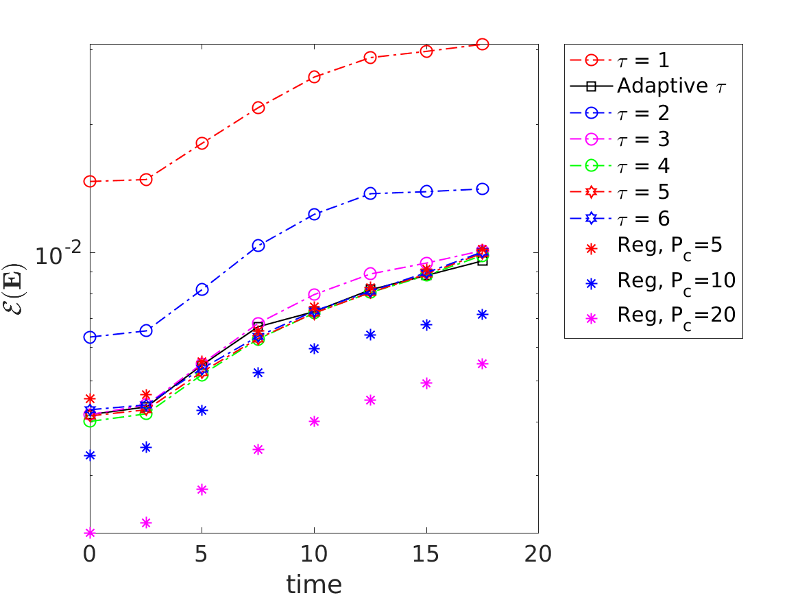
(b) $512^{2}$, $P_{c}=5$

(c) $1024^{2}$, $P_{c}=5$

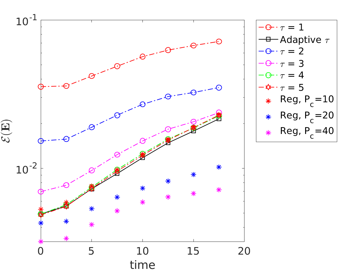
(d) $256^{2}$, $P_{c}=10$

(e) $512^{2}$, $P_{c}=10$

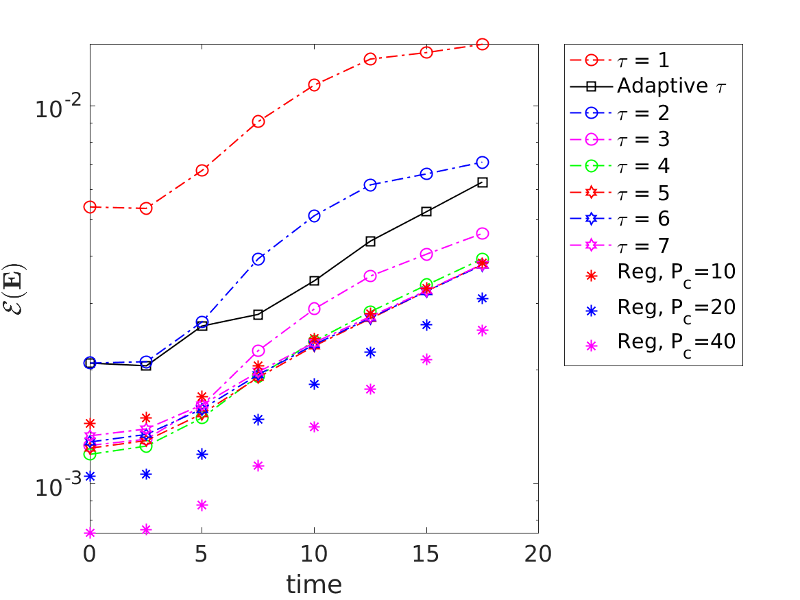
(f) $1024^{2}$, $P_{c}=10$

(g) $256^{2}$, $P_{c}=20$

(h) $512^{2}$, $P_{c}=20$

(i) $1024^{2}$, $P_{c}=20$

Figure 7: 2D diocotron instability. Gaussian sampling: Electric field error comparison between regular (Reg), fixed $\tau$ and adaptive $\tau$ PIC.

In Figure 7, the error in the electric field $\mathbf{E}$ calculated using equation (13) is shown for the meshes and $P_{c}$ considered. We can see that the adaptive $\tau$ errors at the best are similar to the regular PIC and in some cases it is higher than regular PIC error for the same $P_{c}$. We also notice that none of the fixed $\tau$ error levels are better than the regular PIC errors. The reason for this is as follows: the electric field is obtained by integrating the charge density, and integration is a smoothing operation which reduces the particle noise. Since in our adaptive $\tau$ noise reduction algorithm we increase the grid-based error to reduce the particle noise and minimize the total error in the density, this can result in either similar or even an increase in the electric field error as compared to the regular PIC if the integration itself is sufficient enough to reduce the noise. High-order shape functions are a promising option to address this limitation as they may reduce the particle noise without increasing the grid-based error. We will investigate the combination of high-order shape functions with our algorithm in future work.

(a) $256^{2}$, $P_{c}=5$

(b) $512^{2}$, $P_{c}=5$

(c) $1024^{2}$, $P_{c}=5$

(d) $256^{2}$, $P_{c}=10$

(e) $512^{2}$, $P_{c}=10$

(f) $1024^{2}$, $P_{c}=10$

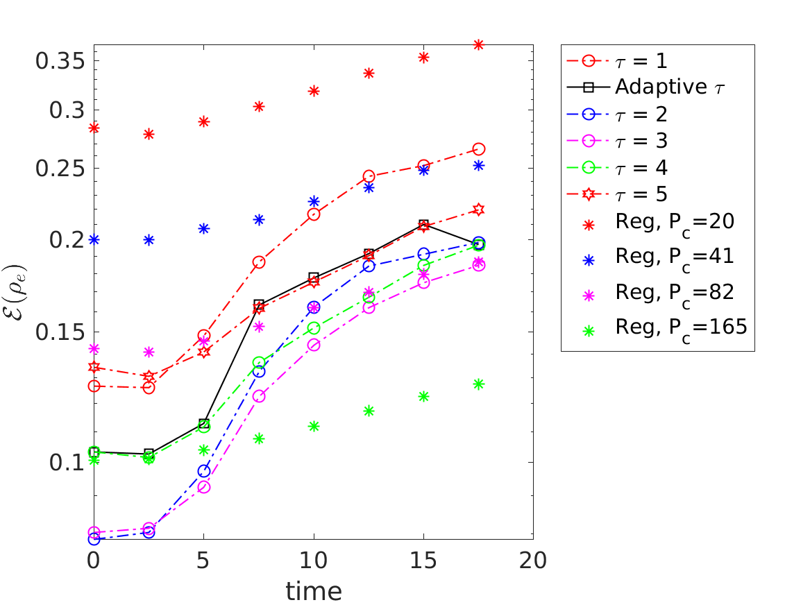
(g) $256^{2}$, $P_{c}=20$

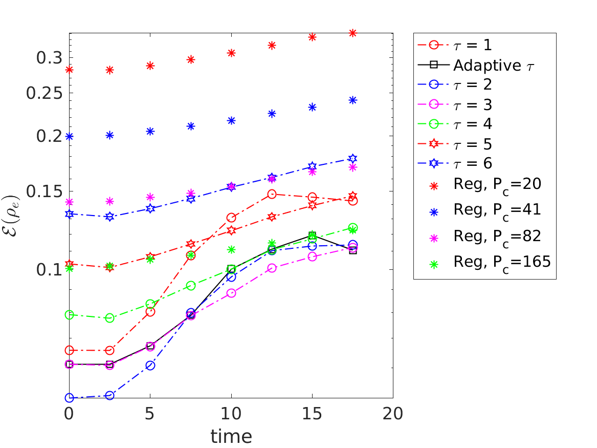
(h) $512^{2}$, $P_{c}=20$

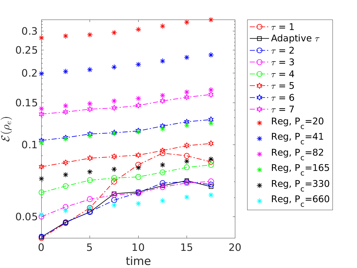
(i) $1024^{2}$, $P_{c}=20$

Figure 8: 2D diocotron instability. Uniform sampling: Electron charge density error comparison between regular (Reg), fixed $\tau$ and adaptive $\tau$ PIC. The errors for regular PIC with $P_{c}=330$ and $660$ are calculated from that of $P_{c}=165$ based on the theoretical particle error scaling $1/\sqrt{Pc}$. This is based on the observation that the errors for the regular PIC are in the noise dominated regime.

(a) $256^{2}$, $P_{c}=5$

(b) $512^{2}$, $P_{c}=5$

(c) $1024^{2}$, $P_{c}=5$

(d) $256^{2}$, $P_{c}=10$

(e) $512^{2}$, $P_{c}=10$

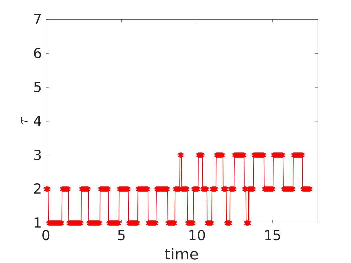
(f) $1024^{2}$, $P_{c}=10$

(g) $256^{2}$, $P_{c}=20$

(h) $512^{2}$, $P_{c}=20$

(i) $1024^{2}$, $P_{c}=20$

Figure 9: 2D diocotron instability. Uniform sampling: Time history of $\tau$ for different mesh sizes and number of particles per cell $P_{c}$.

Having studied the adaptivity of the algorithm with respect to mesh size, $P_{c}$ and time (smoothness of the function) we will now consider a different initial sampling technique and evaluate the performance. To that end, we sample the $f$ in equation (14) with a uniform distribution in all the variables. The range for the velocity variables is chosen as $[-6,6]$ while for the configuration space it is $[0,L]$. Note that unlike the Gaussian sampling described earlier, with this sampling each particle will have a different constant charge $q_{e}$ [11] to match the distribution. But the charge to mass ratio is the same for all the particles. Similar to [18], we ignore particles with weights less than $1.0\times 10^{-9}$. This naive Monte-Carlo sampling strategy, as we will see in the results for this example, has higher noise levels than the Gaussian sampling. However it can be useful in scenarios where we do not know of an importance sampling technique to sample the distribution at hand.

Owing to higher noise levels in the sampling strategy, we needed $(P_{c})_{ref}=5$ and $\alpha=0.03$ for the calculation of the denoising threshold. Figure 8 shows that in general, except for the coarsest mesh size $256^{2}$, the adaptive $\tau$ algorithm performs well in this case also in terms of picking a nearly optimal $\tau$ for most of the cases. The time history of $\tau$ in Figure 9 shows that as expected, the optimal $\tau$ values for this case are lower than that for the Gaussian sampling in Figure 6 due to higher noise levels.

	Gaussian sampling			Uniform sampling
​​​ Mesh	​​$P_{c}$ ​​			​​$P_{c}$ ​​
	5	10	20	5	10	20
$256^{2}$	43.9	47.7	55.5	42.5	44.7	50.3
$512^{2}$	92.2	110	146	85	96	119
$1024^{2}$	435	501.7	654	394.7	438.5	544

Table 1: 2D diocotron instability. Adaptive $\tau$ PIC: Total run time in seconds on 64 cores for different mesh sizes and number of particles per cell for the Gaussian and uniform sampling techniques.

​​​ Mesh	​​Regular PIC ​​			​​Reg/adaptive $\tau$​​
$256^{2}$	51 ($20$)	51 ($20$)	104.7 ($80$)	1.2	1.1	1.9
$512^{2}$	201.7 ($40$)	364.3 ($80$)	709 ($160$)	2.2	3.3	4.8
$1024^{2}$	1543.8 ($80$)	2911.1 ($160$)	5857 ($320$)	3.5	5.8	8.9

Table 2: 2D diocotron instability. Gaussian sampling: Columns $2-4$ are the total run time in seconds taken by the regular PIC on 64 cores for different mesh sizes and number of particles per cell (within parentheses) to reach a comparable accuracy (based on visual norm from the left columns of Figures 3-5) in charge density that of the adaptive $\tau$ results in Table 1 at time $T=17.5$. Columns $5-7$ are the ratio of time taken by regular PIC to the values in columns $2-4$ of Table 1 for adaptive $\tau$ PIC.

​​​ Mesh	​​Regular PIC ​​			​​Reg/adaptive $\tau$ ​​
$256^{2}$	45.7 ($20$)	56.1 ($41$)	80.1 ($82$)	1.1	1.2	1.6
$512^{2}$	249.3 ($82$)	462.9 ($165$)	462.9 ($165$)	2.9	4.8	3.9
$1024^{2}$	1926 ($165$)	3665.4 ($330$)	6964.3 ($660$)	4.9	8.3	12.8

Table 3: 2D diocotron instability. Uniform sampling: Columns $2-4$ are the total run time in seconds taken by the regular PIC on 64 cores for different mesh sizes and number of particles per cell (within parentheses) to reach a comparable accuracy (based on visual norm from Figure 8) in charge density that of the adaptive $\tau$ results in Table 1 at time $T=17.5$. Columns $5-7$ are the ratio of time taken by regular PIC to the values in columns $5-7$ of Table 1 for adaptive $\tau$ PIC. The timing reported for $P_{c}=660$ and hence the speedup corresponding to it is a theoretically extrapolated one obtained by multiplying the timing for $P_{c}=330$ with a factor $1.9$ which is the ratio between timings for $P_{c}=330$ to $P_{c}=165$.

Finally, we perform a preliminary run time performance study to see the effectiveness of the current approach in comparison to the regular PIC. To that extent, we note that we did not perform any optimization to both the regular PIC as well as the adaptive $\tau$ PIC routines. Optimization of different components involved in the algorithm as well as a thorough parallel performance study is left for future work. In Table 1 the total run time in seconds is shown for the adaptive $\tau$ PIC on 64 cores for the mesh sizes, $P_{c}$ and sampling techniques considered before. All the timings reported are the average of three runs performed. In Tables 2 and 3, we compare the adaptive $\tau$ PIC timings with the timings for the regular PIC with the $P_{c}$ value required to reach a comparable accuracy in charge density as that of the adaptive $\tau$ results at final time $T=17.5$. The approximate $P_{c}$ values within parentheses are obtained from Figures 3-5 and Figure 8 based on visual examination. Even in this preliminary performance study, we can see that the adaptive $\tau$ strategy can provide significant speedups up to an order of magnitude compared to the regular PIC for similar accuracy in charge density. In terms of memory storage, the benefits are even more pronounced. Using the number of particles $N_{p}$ as a measure of the dominant memory cost (for PIC methods this is usually the case) we see $\approx 2-16$ times memory reduction (in case of Gaussian sampling) and $\approx 4-33$ times memory reduction (in case of uniform sampling) with adaptive $\tau$ PIC compared to regular PIC.

5.2 3D Penning trap

In this section we will consider a 3D Penning trap problem as the test case. Penning traps are storage devices for charged particles, which uses a quadrupole electric field to confine the particles axially and a homogeneous axial magnetic field to confine the particles in the radial direction [50, 51]. The evolution of the density in this problem (see Figure 10) is very similar to that observed in cyclotrons [52, 53]. Thus this test case is very relevant to our ultimate goal of high precision large-scale simulation of cyclotrons. The fine scale structures developed in this problem pose challenges for the sparse grids similar to the diocotron case in the previous section.

The parameters for this test case are as follows. The length of the periodic box is $L=20$. The external magnetic field is given by $\mathbf{B}_{ext}=\left\{0,0,5\right\}$ and the quadrupole external electric field by

$$\mathbf{E}_{ext}=\left\{-\frac{15}{L}\left(x-\frac{L}{2}\right),-\frac{15}{L}\left(y-\frac{L}{2}\right),\frac{30}{L}\left(z-\frac{L}{2}\right)\right\}.$$

For the initial conditions, we sample the phase space using a Gaussian distribution in all the variables. The mean and standard deviation for all the velocity variables is $0$ and $1$ respectively. While the mean for all the configuration space variables is $L/2$ the standard deviations are $0.15L$, $0.05L$ and $0.2L$ for $x$, $y$ and $z$ respectively. The total electron charge is $Q_{e}=-1562.5$, and the charge of each particle is $q_{e}=\frac{Q_{e}}{N_{p}}$.

The denoising parameters are taken as $(P_{c})_{ref}=1$ and $\alpha=0.005$ for this problem with the above mentioned sampling. The time step is chosen as $\Delta t=0.05$ and the simulations are run till final time $T=15$.

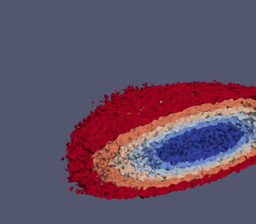
(a) time=0

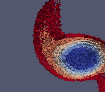
(b) time=10

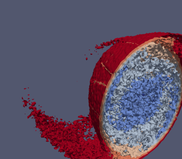
(c) time=15

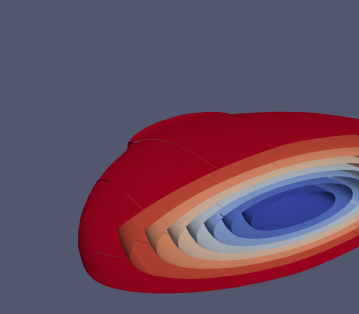
(d) time=0

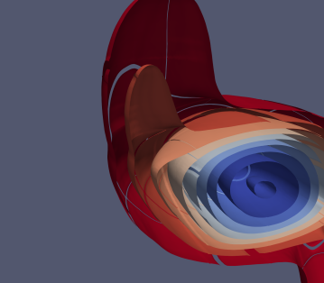
(e) time=10

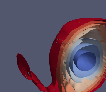
(f) time=15

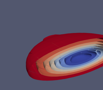
(g) time=0

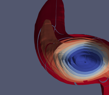
(h) time=10

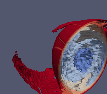
(i) time=15

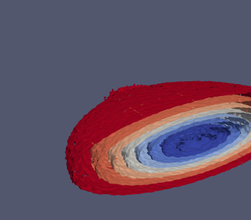
(j) time=0

(k) time=10

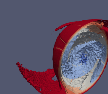
(l) time=15

Figure 10: 3D Penning trap: Evolution of the electron charge density with time for regular PIC, $P_{c}=1$ (first row); $\tau=1$, $P_{c}=1$ (second row); adaptive $\tau$, $P_{c}=1$ (third row); and regular PIC, $P_{c}=20$ (fourth row). The mesh considered here is $256^{3}$.

Figure 10 shows the evolution of the electron charge density with time for regular, $\tau=1$ and adaptive $\tau$ PIC. The mesh used is $256^{3}$ and $P_{c}=1$ for the first three rows and $20$ for the last row. As we had seen in Figure 2 for the diocotron test case, the adaptive $\tau$ results, in the third row are better than both the regular PIC and $\tau=1$ results and are comparable to the results of the regular PIC with higher $P_{c}$ in the last row.

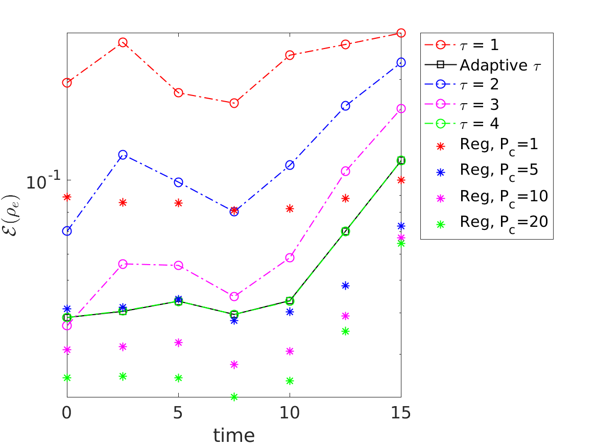
(a) $64^{3}$, $P_{c}=1$

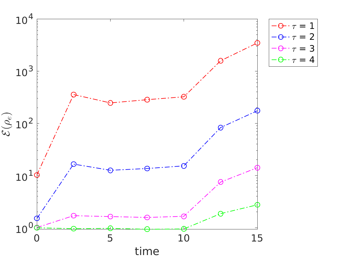
(b) $64^{3}$, $P_{c}=1$

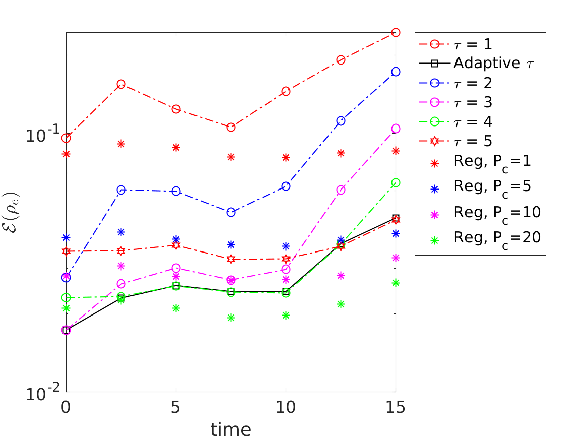
(c) $128^{3}$, $P_{c}=1$

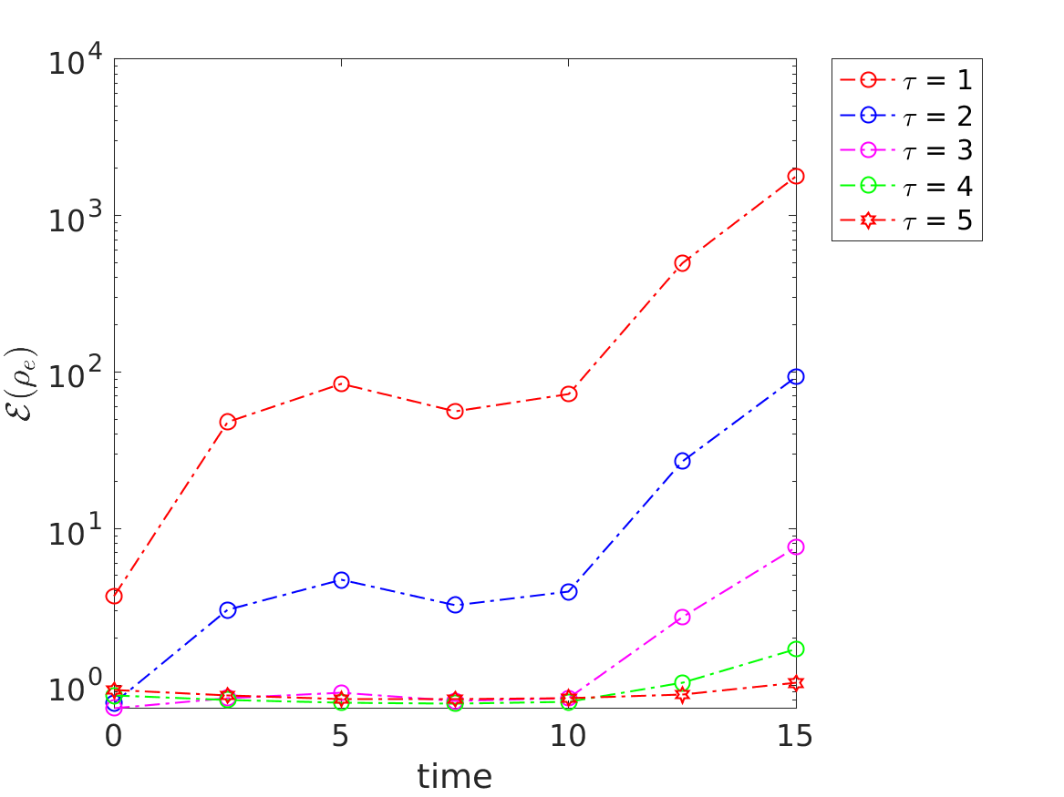
(d) $128^{3}$, $P_{c}=1$

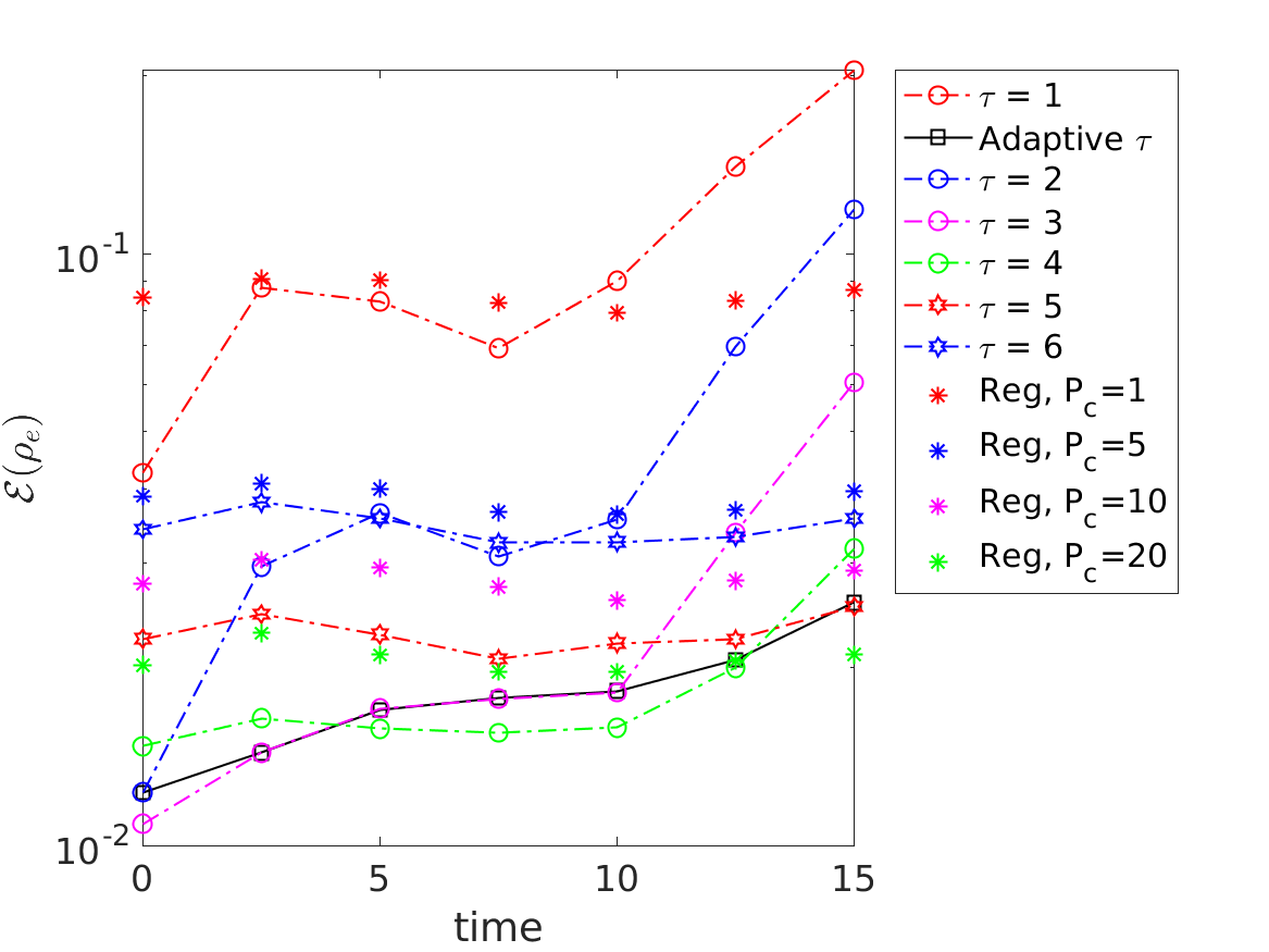
(e) $256^{3}$, $P_{c}=1$

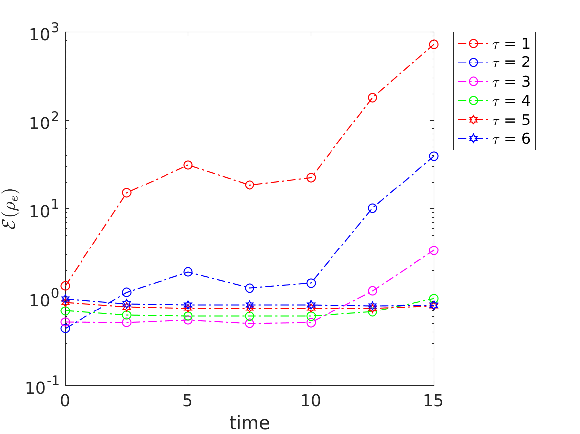
(f) $256^{3}$, $P_{c}=1$

Figure 11: 3D Penning trap: Electron charge density error comparison between regular (Reg), fixed $\tau$ and adaptive $\tau$ PIC. The left column is the actual error calculated using equation (13) and the right column is the estimations from the $\tau$ estimator based on which the optimal $\tau$ is selected. The fixed as well as adaptive $\tau$ has the number of particles per cell $P_{c}=1$.

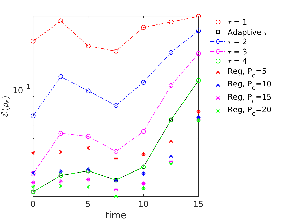
(a) $64^{3}$, $P_{c}=5$

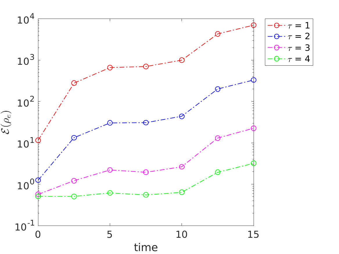
(b) $64^{3}$, $P_{c}=5$

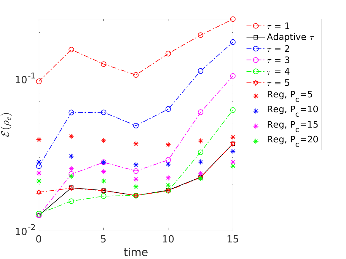
(c) $128^{3}$, $P_{c}=5$

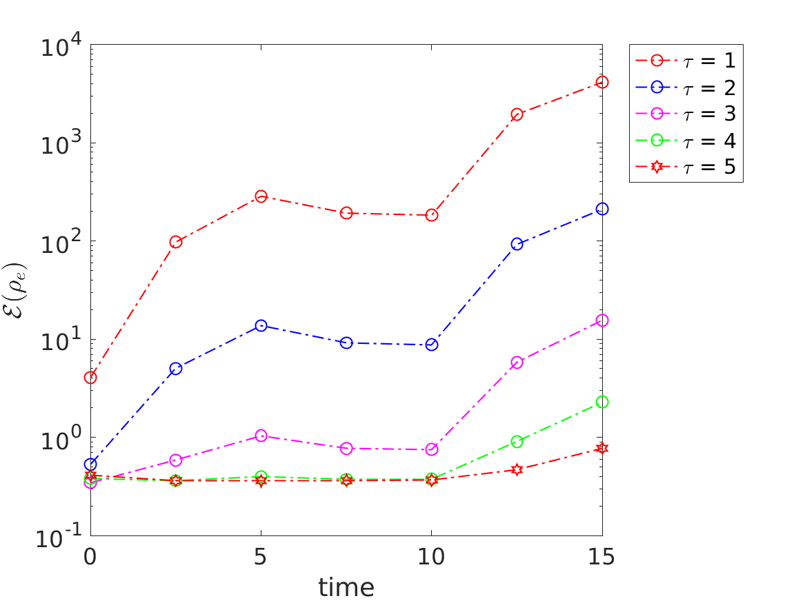
(d) $128^{3}$, $P_{c}=5$

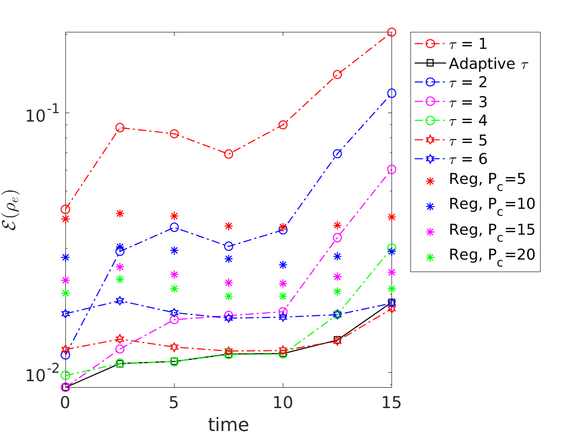
(e) $256^{3}$, $P_{c}=5$

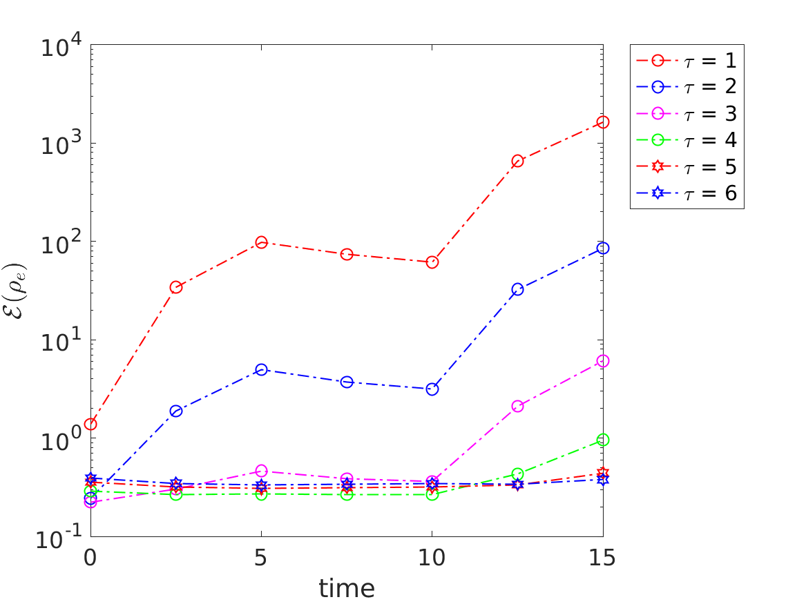
(f) $256^{3}$, $P_{c}=5$

Figure 12: 3D Penning trap: Electron charge density error comparison between regular (Reg), fixed $\tau$ and adaptive $\tau$ PIC. The left column is the actual error calculated using equation (13) and the right column is the estimations from the $\tau$ estimator based on which the optimal $\tau$ is selected. The fixed as well as adaptive $\tau$ has the number of particles per cell $P_{c}=5$.

In a way analogous to Figures 3-5 for the diocotron instability, in Figures 11-12 we show the errors calculated using equation (13) and the estimations from the $\tau$ estimator for meshes $64^{3},128^{3},256^{3}$ and $P_{c}=1,5$. The reference in equation (13) is the average of 5 independent computations of regular PIC with $256^{3}$ mesh and $P_{c}=40$. For the $N_{points}$ in equation (13), we select approximately $4096$ random points throughout the domain and interpolate both the reference density as well as the density under consideration at these points to measure the error. The errors are measured at 7 time instants in the simulation.

In general, as before the adaptive $\tau$ predictions are close to optimal and most of the conclusions from the diocotron test case are applicable in this case too. Figure 13 shows the time history of $\tau$ for the meshes and $P_{c}$ considered and the high values of $\tau$ indicate that the total error is dominated by the grid-based error in these cases.

(a) $64^{3}$, $P_{c}=1$

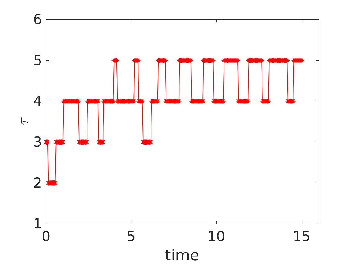
(b) $128^{3}$, $P_{c}=1$

(c) $256^{3}$, $P_{c}=1$

(d) $64^{3}$, $P_{c}=5$

(e) $128^{3}$, $P_{c}=5$

(f) $256^{3}$, $P_{c}=5$

Figure 13: 3D Penning trap: Time history of $\tau$ for different mesh sizes and number of particles per cell $P_{c}$.

In terms of run time performance comparisons, we ran the $64^{3},128^{3}$ mesh cases on 64 cores and the $256^{3}$ test cases on 512 cores for both the regular and adaptive $\tau$ PIC. For $64^{3}$ mesh, at the last time instant we can see that the regular PIC is more accurate than the adaptive $\tau$ or any other fixed $\tau$ PIC.

	Adaptive $\tau$		Regular		Reg/adaptive $\tau$
$128^{3}$	361 ($1$)	476 ($5$)	273 ($5$)	444 ($10$)	0.8	0.9
$256^{3}$	829 ($1$)	1201 ($5$)	2360 ($15$)	3081 ($20$)	2.8	2.6

Table 4: 3D Penning Trap: Total run time in seconds on 64 cores for $128^{3}$ mesh and 512 cores for $256^{3}$ mesh in case of the regular and adaptive $\tau$ PIC. The values within the parentheses represent the different number of particles per cell required to reach a comparable accuracy (based on visual norm from the left columns of Figures 11-12) in the charge density for both the schemes at final time $T=15$. Columns $6-7$ are the ratio of time taken by the regular PIC to that for adaptive $\tau$ PIC.

For $128^{3}$ and $256^{3}$ meshes, from Table 4 we can see a maximum speedup of $2.8$ with adaptive $\tau$ PIC over the regular PIC for the finest mesh size. Again considering the number of particles as a measure for the memory cost adaptive $\tau$ PIC is $2-15$ times cheaper than the regular PIC. In order to see more computational benefits with the adaptive $\tau$ PIC for this problem we need to perform runs with finer meshes and more particles per cell. These 3D large-scale simulations are part of our future work and the results will be reported elsewhere.

6 Conclusions

We have proposed a sparse grids based adaptive noise reduction strategy for particle-in-cell (PIC) simulations. Unlike the typical physical or Fourier domain filters used in PIC methods, the strategy adapts to mesh size, number of particles per cell, smoothness of the charge density and the initial sampling technique. In order to construct the strategy we use the key idea of increased particles per cell in sparse grids compared to the regular grid for the same total number of particles as proposed in [1]. The current work extends that concept in several directions. Specifically, we present a filtering perspective for the sparse grids based noise reduction which helps to incorporate it with ease in existing high performance large-scale PIC code bases and also opens the door for sparse grids based filtering approaches. We tackle the problem of large grid-based error of sparse grids for non-aligned and non-smooth functions by means of the truncated combination technique [2, 3, 4]. We show in the context of PIC simulations that the truncated combination technique provides a natural framework to minimize the sum of grid-based error and particle noise. This allows us to propose a heuristic based on formal error analysis to select the optimal truncation parameter on the fly that minimizes the total error.

We show the performance and applicability of our strategy on two benchmark problems; namely the 2D diocotron instability and electron dynamics in a 3D Penning trap. In both test cases the adaptive noise reduction strategy picks a truncation parameter which is close to optimal for all times. To achieve comparable accuracy for the charge density deposition we obtain significant speedups and memory savings up to an order of magnitude with the noise reduction technique compared to regular PIC in the 2D diocotron test case. For the 3D Penning trap test case a maximum speedup of $2.8$ and $15$ times memory reduction is obtained for the finest mesh size tested. Further speedups and memory reduction in the 3D test case require us to test the strategy for even finer resolutions and that is part of future work.

Our strategy can be very easily integrated into existing high performance large-scale PIC code bases and ongoing work is to integrate it into the open source particle accelerator library OPAL [27]. In terms of future work, we plan on investigating the applicability and performance of the noise reduction strategy on large-scale high intensity particle accelerator simulations such as the IsoDAR project [54, 55] with a particular focus on understanding the dynamics of halo particles and efficient collimation strategies. Filtering strategies have much more impact on the electromagnetic PIC simulations as reported in [22]. Hence we would like to extend the current approach for Vlasov-Maxwell equations and investigate the performance in that context. Use of machine learning approaches to tune denoising threshold in our strategy is also of interest. Finally, we also intend to compare the current strategy with other filtering approaches and denoising techniques.

Appendix A. Proof of Proposition 1 relating the direct charge density deposition onto the component grids and the two-step approach

Proof.

Even though sparse grids make sense only for dimensions 2 and higher we can still understand the essence of the proof in 1D. Also, since the shape functions and transfer operators in 2D and 3D are obtained by the tensor product of 1D linear interpolation functions the proof extends naturally to those cases.

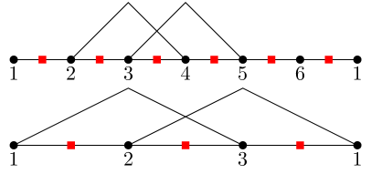
(a) Node-centered grid

(b) Cell-centered grid

Figure 14: Schematic showing the node-centered and cell-centered grids and the corresponding shape functions. The nodes are marked with black circles and the cell-centers with red squares. The domain is periodic. The shape functions $W_{c}$ corresponding to the coarse grid are linear between the nodes in the fine grid in case of node-centered grids. For cell-centered grids $W_{c}$ has discontinuity in derivative between some of the cell-centers in the fine grid whereas between nodes of the fine grid it is always linear.

Consider a periodic 1D domain $[0,L]$ and two grids with mesh sizes $h_{f}$ and $h_{c}$. The grid with mesh size $h_{c}$ is coarser than the one with $h_{f}$ and assume $h_{c}$ is an integer multiple of $h_{f}$. Let us first consider the node-centered grids where all the coarse grid points are also grid points in the fine grid as shown in Figure 14(a).

The particles deposit onto the fine grid with mesh size $h_{f}$ and the charge density $\tilde{\rho}_{e}$ is given by

$$\tilde{\rho}_{e}(\tilde{x}_{j})=\frac{Q_{e}}{N_{p}h_{f}}\sum_{p=1}^{N_{p}}W_{f}(\tilde{x}_{j}-x_{p}),$$ (15)

where $W_{f}(\zeta)=\max\left\{0,1-\frac{|\zeta|}{h_{f}}\right\}$ is the cloud-in-cell shape function and $x_{p}$ and $\tilde{x}_{j}$ are the locations of the particles and the grid points in the fine grid respectively. Now, we transfer the density $\tilde{\rho}_{e}$ to the coarse grid by means of the transfer operator $R$ in equation (3) which gives

$$\varrho_{e}(x_{k})=\frac{h_{f}}{h_{c}}\sum_{j=1}^{N_{c}}\tilde{\rho}_{e}(\tilde{x}_{j})W_{c}(x_{k}-\tilde{x}_{j}),$$ (16)

where $W_{c}(\zeta)=\max\left\{0,1-\frac{|\zeta|}{h_{c}}\right\}$, $x_{k}$ are the locations of the grid points in the coarse grid and $N_{c}$ is the total number of cells in the fine grid. Substituting for $\tilde{\rho}_{e}$ from equation (15) and switching the order of sums we get

$$\varrho_{e}(x_{k})=\frac{Q_{e}}{N_{p}h_{c}}\sum_{p=1}^{N_{p}}\sum_{j=1}^{N_{c}}W_{c}(x_{k}-\tilde{x}_{j})W_{f}(\tilde{x}_{j}-x_{p}).$$ (17)

Now, for a given particle, $W_{f}(\tilde{x}_{j}-x_{p})$ is non-zero for exactly two values of $j$: the floor of $x_{p}/h_{f}$ and the ceiling of that same quantity. Let us call these values $J$ and $J+1$ and assume the grid points are ordered such that $x_{J}$ is to the left of $x_{J+1}$. We have

$$\sum_{j=1}^{N_{c}}W_{c}(x_{k}-\tilde{x}_{j})W_{f}(\tilde{x}_{j}-x_{p}) =W_{c}(x_{k}-\tilde{x}_{J})W_{f}(\tilde{x}_{J}-x_{p})$$

$$+W_{c}(x_{k}-\tilde{x}_{J+1})W_{f}(\tilde{x}_{J+1}-x_{p}).$$ (18)

Now we note that because of the way the two grids are related (mesh sizes are integer multiples, coincident grid points), we are guaranteed that $W_{c}(x_{k}-\tilde{x})$ is linear on the interval $\tilde{x}\in[\tilde{x}_{J},\tilde{x}_{J+1}]$. This is because the places where $W_{c}$ has a discontinuity in its derivative are guaranteed to be fine grid points as shown in Figure 14(a). So, linear interpolation is exact for $W_{c}$ on the interval $[\tilde{x}_{J},\tilde{x}_{J+1}]$. Since $x_{p}$ is in this interval, we have

$$W_{c}(x_{k}-x_{p})=W_{c}(x_{k}-\tilde{x}_{J})\left[\frac{\tilde{x}_{J+1}-x_{p}}{\tilde{x}_{J+1}-\tilde{x}_{J}}\right]+W_{c}(x_{k}-\tilde{x}_{J+1})\left[1-\frac{\tilde{x}_{J+1}-x_{p}}{\tilde{x}_{J+1}-\tilde{x}_{J}}\right].$$

Now we notice that

$$\left[\frac{\tilde{x}_{J+1}-x_{p}}{\tilde{x}_{J+1}-\tilde{x}_{J}}\right]=\left[\frac{\tilde{x}_{J}+h_{f}-x_{p}}{h_{f}}\right]=1+\frac{\tilde{x}_{J}-x_{p}}{h_{f}}=1-\frac{|\tilde{x}_{J}-x_{p}|}{h_{f}}=W_{f}(\tilde{x}_{J}-x_{p}),$$

and a nearly identical reasoning gives

$$\left[1-\frac{\tilde{x}_{J+1}-x_{p}}{\tilde{x}_{J+1}-\tilde{x}_{J}}\right]=W_{f}(\tilde{x}_{J+1}-x_{p}).$$

Combining these with equation (18) we get

$$\sum_{j=1}^{N_{c}}W_{c}(x_{k}-\tilde{x}_{j})W_{f}(\tilde{x}_{j}-x_{p})=W_{c}(x_{k}-x_{p}).$$ (19)

Substituting this into equation (17) we get the density on the coarse grid as

$$\varrho_{e}(x_{k})=\frac{Q_{e}}{N_{p}h_{c}}\sum_{p=1}^{N_{p}}W_{c}(x_{k}-x_{p}).$$ (20)

Comparing equation (20) with equation (15) we see this is exactly the expression we would obtain if the particles were to deposit directly onto the coarse grid with mesh size $h_{c}$.

Now we will consider the cell-centered grids. In this case the coarse grid points are also not the grid points in the fine grid and $W_{c}$ will have a discontinuity in the derivative for some of the intervals $[\tilde{x}_{j},\tilde{x}_{j+1}]$ as shown in Figure 14(b) depending on the ratio $h_{c}/h_{f}$. Hence an exact equivalence between the two approaches does not hold. However, we will now show that

$$\mathcal{W}_{c}(x_{k}-x)=\sum_{j=1}^{N_{c}}W_{c}(x_{k}-\tilde{x}_{j})W_{f}(\tilde{x}_{j}-x)$$

can be considered as a shape function by itself. To that end, we will show that it satisfies the three conditions for any shape function as given in [56]. These are listed as follows

1. $\mathcal{W}_{c}(\zeta)=\mathcal{W}_{c}(-\zeta)$,

2. $\frac{1}{h_{c}}\int\mathcal{W}_{c}(\zeta)d\zeta=1$,

3. $\sum\limits_{k}\mathcal{W}_{c}(x_{k}-x)=1$.

The first condition is manifestly true as $W_{f}$ which is the standard hat function is even. For the second condition we observe that

$$\frac{1}{h_{c}}\int\mathcal{W}_{c}(\zeta)d\zeta=\frac{h_{f}}{h_{c}}\sum_{j=1}^{N_{c}}W_{c}(x_{k}-\tilde{x}_{j}),$$

as $W_{f}$ is a shape function and by definition integrates to $h_{f}$. Now, $h_{f}\sum_{j=1}^{N_{c}}W_{c}(x_{k}-\tilde{x}_{j})$ is the midpoint rule applied for the integration $\int W_{c}(x_{k}-\tilde{x})$ over the fine grid. From Figure 14(b) it is clear that $W_{c}$ is linear on each integration cell and the midpoint rule is exact. Thus,

$$\frac{h_{f}}{h_{c}}\sum_{j=1}^{N_{c}}W_{c}(x_{k}-\tilde{x}_{j})=\frac{1}{h_{c}}\int W_{c}(x_{k}-\tilde{x})d\tilde{x}=1,$$

where the last step comes from the fact that $W_{c}$ which is also a standard hat function integrates to $h_{c}$ by definition. Finally, the third condition is related to global charge conservation and we note that since $W_{c}$ and $W_{f}$ are standard hat functions they satisfy the partition of unity and hence $\mathcal{W}_{c}$ also satisfies it when we carry out the summation.

Now, using conditions 1 and 2 and noting that $\mathcal{W}_{c}$ is bounded in $[0,L]$ we can carry out the same set of steps shown in appendix B for a standard hat function. We can then see the grid-based error for $\mathcal{W}_{c}$ is of $\mathcal{O}(\left\lvert\partial^{2}_{x}\rho_{e}\right\rvert h_{c}^{2})$ and the particle noise is $\mathcal{O}(\sqrt{\left\lvert Q_{e}\rho_{e}\right\rvert/N_{p}h_{c}})$ as in equations (31) and (47) but with the constants depending on the ratio of $h_{c}$ to $h_{f}$. ∎

Appendix B. Grid-based and particle errors in the charge density deposition for regular PIC schemes

In this section, we follow the analysis in [1] and derive in details the grid-based error and noise estimates for the charge density deposition in regular PIC schemes explicitly revealing the constants. For simplicity, let us consider a 1D PIC scheme and extensions to 2D and 3D are relatively straightforward. In the following, we consider a particular time instant and hence suppress the dependence of the different quantities with respect to time.

Let $f(x,v)$ be the electron phase-space distribution under consideration and let us define ${\bar{f}}$ as

$${\bar{f}}=\frac{f}{\int\int fdxdv}.$$

Since, ${\bar{f}}$ is non-negative and its phase-space integral is unity it can be interpreted as probability density. The exact charge density $\rho_{e}(x)$ is given by

$$\rho_{e}(x) =q_{e}\int\int f({\xi},v)\delta(x-\xi)d\xi dv,$$ (21)

$$=q_{e}\left(\int\int fdxdv\right)\int\int{\bar{f}}(\xi,v)\delta(x-\xi)d\xi dv,$$ (22)

$$=Q_{e}\int\int{\bar{f}}(\xi,v)\delta(x-\xi)d\xi dv,$$ (23)

where $Q_{e}=q_{e}\int\int fdxdv$ is the total electron charge in the system and $\delta(x-\xi)$ is the Dirac delta function.

In PIC, we approximate $\delta(x-\xi)$ with the shape function $S(x-\xi)$ which for our discussion here consider it to be the cloud-in-cell or linear interpolation function. The approximate charge density $\bar{\rho}_{e}$ with the shape function $S(x-\xi)$ is given by

$$\bar{\rho}_{e}(x) =Q_{e}\int\int{\bar{f}}(\xi,v)S(x-\xi)d\xi dv,$$ (24)

$$=Q_{e}\mathbb{E}_{{\bar{f}}(\xi,v)}\left[S(x-\xi)\right],$$ (25)

where $\mathbb{E}$ is the expected value over the probability density ${\bar{f}}$.

B.1 Grid-based error estimate

This is the error due to approximating $\delta(x-\xi)$ with the shape function $S(x-\xi)$

$$e_{g}=\left\lvert\rho_{e}-\bar{\rho}_{e}\right\rvert.$$ (26)

Towards estimating this error, let us expand ${\bar{f}}(\xi,v)$ in equation (24) in terms of Taylor’s series about $x$,

$$\bar{\rho}_{e} =Q_{e}\int\int\left({\bar{f}}(x,v)+(\xi-x)\partial_{x}{\bar{f}}(x,v)\right.$$

$$+\left.\frac{(\xi-x)^{2}}{2}\partial^{2}_{x}{\bar{f}}(x,v)+\cdots\right)S(x-\xi)d\xi dv,$$ (27)

$$=\underbrace{Q_{e}\int{\bar{f}}dv}_{\rho_{e}}\underbrace{\int S(x-\xi)d\xi}_{1}+Q_{e}\int\partial_{x}{\bar{f}}dv\int(\xi-x)S(x-\xi)d\xi$$

$$+Q_{e}\int\partial^{2}_{x}{\bar{f}}dv\int\frac{(\xi-x)^{2}}{2}S(x-\xi)d\xi+\cdots,$$ (28)

where we have used the fact that the integral of the shape function $S(x-\xi)$ is unity. In the above equations we have used the short hand notations $\partial_{x}=\frac{\partial(.)}{\partial x}$ and $\partial^{2}_{x}=\frac{\partial^{2}(.)}{\partial x^{2}}$. Taking outside the partial derivatives with respect to $x$ in the $\int dv$ integrals we get

$$\bar{\rho}_{e}=\rho_{e}+\partial_{x}\rho_{e}\int(\xi-x)S(x-\xi)d\xi+\partial^{2}_{x}\rho_{e}\int\frac{(\xi-x)^{2}}{2}S(x-\xi)d\xi+\cdots.$$ (29)

The cloud-in-cell shape function is given by

$$S(\zeta)=\frac{1}{h_{x}}\max\left\{0,1-\frac{\left\lvert\zeta\right\rvert}{h_{x}}\right\}.$$ (30)

Performing a change of variables with $\zeta=\xi-x$ in equation (29) and noting that $S(\zeta)$ has a compact support and is zero outside $|\zeta|\leq h_{x}$ all the integrals has to be carried only in $-h_{x}\leq\zeta\leq h_{x}$.

Also, $S(\zeta)$ is an even function and hence $\int_{-h_{x}}^{h_{x}}\zeta S(\zeta)d\zeta$ which is the second term in equation (29) is 0. However, the integrand in the third term of the equation (29) is an even function and it evaluates to

$$\int\frac{(\xi-x)^{2}}{2}S(x-\xi)d\xi=\frac{1}{h_{x}}\int_{0}^{h_{x}}\zeta^{2}\left(1-\frac{\zeta}{h_{x}}\right)d\zeta=\frac{h_{x}^{2}}{12}.$$

Thus equation (26) becomes

$$e_{g}(x) \leq\frac{h_{x}^{2}}{12}\left\lvert\partial^{2}_{x}\rho_{e}(x)\right\rvert+\cdots,$$

$$e_{g} =\mathcal{O}\left(\frac{h_{x}^{2}}{12}\left\lvert\partial^{2}_{x}\rho_{e}(x)\right\rvert\right).$$ (31)

Since, the cloud-in-cell shape functions in 2D and 3D are obtained by the tensor product of 1D shape functions the analysis extends easily to these cases. Carrying out similar steps we obtain the grid-based error for 2D and 3D as

$$e_{g} =\mathcal{O}\left(\frac{1}{12}\left\{\left\lvert\frac{\partial^{2}\rho_{e}}{\partial x^{2}}\right\rvert h_{x}^{2}+\left\lvert\frac{\partial^{2}\rho_{e}}{\partial y^{2}}\right\rvert h_{y}^{2}\right\}+\frac{1}{144}\left\lvert\frac{\partial^{4}\rho_{e}}{\partial x^{2}\partial y^{2}}\right\rvert h_{x}^{2}h_{y}^{2}\right)\quad\text{in 2D,}$$ (32)

$$e_{g} =\mathcal{O}\left(\frac{1}{12}\left\{\left\lvert\frac{\partial^{2}\rho_{e}}{\partial x^{2}}\right\rvert h_{x}^{2}+\left\lvert\frac{\partial^{2}\rho_{e}}{\partial y^{2}}\right\rvert h_{y}^{2}+\left\lvert\frac{\partial^{2}\rho_{e}}{\partial z^{2}}\right\rvert h_{z}^{2}\right\}\right.$$

$$+\left.\frac{1}{144}\left\{\left\lvert\frac{\partial^{4}\rho_{e}}{\partial x^{2}\partial y^{2}}\right\rvert h_{x}^{2}h_{y}^{2}+\left\lvert\frac{\partial^{4}\rho_{e}}{\partial y^{2}\partial z^{2}}\right\rvert h_{y}^{2}h_{z}^{2}+\left\lvert\frac{\partial^{4}\rho_{e}}{\partial z^{2}\partial x^{2}}\right\rvert h_{z}^{2}h_{x}^{2}\right\}\right.$$

$$+\left.\frac{1}{1728}\left\lvert\frac{\partial^{6}\rho_{e}}{\partial x^{2}\partial y^{2}\partial z^{2}}\right\rvert h_{x}^{2}h_{y}^{2}h_{z}^{2}\right)\quad\text{in 3D}.$$ (33)

Note in the above equations the reason for including the only higher order terms proportional to the mixed derivatives is because these terms will contribute to the dominant error for the sparse grid combination. Hence, the constants in front of these terms are of interest for estimating the coefficients of the grid-based error in section 4.3.3.

B.2 Noise estimate

This is the error which occurs when we approximate the expected value of the shape function by means of an arithmetic mean over the number of discrete particles. Thus equation (25) becomes

$$\bar{\rho}_{e}(x)\approx\tilde{\rho}_{e}(x)=\frac{Q_{e}}{N_{p}}\sum_{p}S(x-x_{p}).$$ (34)

The error incurred by this approximation $\eta(x)$ is a random variable with mean 0 and variance given by

$$Var_{{\bar{f}}}\left[\eta(x)\right] =\mathbb{E}_{{\bar{f}}}\left[\left(\bar{\rho}_{e}-\tilde{\rho}_{e}\right)^{2}\right],$$ (35)

$$=\bar{\rho}_{e}^{2}-2\bar{\rho}_{e}\mathbb{E}_{{\bar{f}}}[\tilde{\rho}_{e}]+\mathbb{E}_{{\bar{f}}}[\tilde{\rho}_{e}^{2}],$$ (36)

$$=\mathbb{E}_{{\bar{f}}}[\tilde{\rho}_{e}^{2}]-\bar{\rho}_{e}^{2}.$$ (37)

Here, in equation (37) we used the fact that $\mathbb{E}_{{\bar{f}}}[\tilde{\rho}_{e}]=\mathbb{E}_{{\bar{f}}}[\bar{\rho}_{e}]=\bar{\rho}_{e}$. Let us compute $\mathbb{E}_{{\bar{f}}}\left[\tilde{\rho}_{e}^{2}\right]$

$$\mathbb{E}_{{\bar{f}}}\left[\tilde{\rho}_{e}^{2}\right]=\mathbb{E}_{{\bar{f}}}\left[\frac{Q_{e}^{2}}{{N_{p}}^{2}}\left(\sum_{p}S(x-x_{p})\right)^{2}\right].$$ (38)

Similar to [1] we assume that the initial particle states have been chosen by independent sampling from ${\bar{f}}(t=0)$ and also they remain approximately independent for $N_{p}\gg 1$. Then $\mathbb{E}_{{\bar{f}}}\left[S(x-x_{p})S(x-x_{q})\right]=0$ if $p\neq q$ and all the cross terms vanish giving

$$\mathbb{E}_{{\bar{f}}}\left[\tilde{\rho}_{e}^{2}\right] =\frac{Q_{e}^{2}}{{N_{p}}^{2}}\sum_{p}\mathbb{E}_{{\bar{f}}}\left[\left(S(x-x_{p})\right)^{2}\right],$$ (39)

$$=\frac{Q_{e}^{2}}{{N_{p}}}\mathbb{E}_{{\bar{f}}}\left[\left(S(x-x_{p})\right)^{2}\right],$$ (40)

where, we have used the fact that each particle has same $\mathbb{E}_{{\bar{f}}}\left[\left(S(x-x_{p})\right)^{2}\right]$. Now,

$$\frac{Q_{e}^{2}}{{N_{p}}}\mathbb{E}_{{\bar{f}}}\left[\left(S(x-x_{p})\right)^{2}\right] =\frac{Q_{e}^{2}}{{N_{p}}}\int\int{\bar{f}}(x_{p},v)\left(S(x-x_{p})\right)^{2}dx_{p}dv,$$ (41)

$$=\frac{Q_{e}^{2}}{{N_{p}}}\int\int\left({\bar{f}}(x,v)+(x_{p}-x)\partial_{x}{\bar{f}}(x,v)\right.$$

$$+\left.\frac{(x_{p}-x)^{2}}{2}\partial^{2}_{x}{\bar{f}}(x,v)+\cdots\right)\left(S(x-x_{p})\right)^{2}dx_{p}dv,$$ (42)

and similar to the previous exercise for grid-based error the term associated with $(x_{p}-x)\partial_{x}{\bar{f}}(x,v)$ vanishes and the third term evaluates to $\mathcal{O}(h_{x})$. Hence evaluating the leading order term gives

$$\frac{Q_{e}^{2}}{{N_{p}}}\int\int{\bar{f}}(x,v)\left(S(x-x_{p})\right)^{2}dx_{p}dv =\frac{Q_{e}}{N_{p}}\underbrace{\int Q_{e}{\bar{f}}dv}_{\rho_{e}}\int\left(S(x-x_{p})\right)^{2}dx_{p},$$ (43)

$$=\frac{Q_{e}\rho_{e}}{N_{p}}\frac{2}{h_{x}^{2}}\int_{0}^{h_{x}}\left(1-\frac{\zeta}{h_{x}}\right)^{2}d\zeta,$$ (44)

$$=\frac{2}{3}\frac{Q_{e}\rho_{e}}{N_{p}h_{x}}.$$ (45)

Plugging the above term in equation (40) gives

$$\mathbb{E}_{{\bar{f}}}\left[\tilde{\rho}_{e}^{2}\right]=\frac{2}{3}\frac{Q_{e}\rho_{e}}{N_{p}h_{x}}+\mathcal{O}(h_{x})+\cdots.$$ (46)

Omitting the $\bar{\rho}_{e}^{2}$ term in equation (37) as it is small compared to equation (46) and substituting the above expression gives

$$Var_{{\bar{f}}}\left[\eta(x)\right]\approx\frac{2}{3}\frac{Q_{e}\rho_{e}}{N_{p}h_{x}}.$$

Defining the particle noise error $e_{n}$ as the standard deviation of the random variable $\eta$ we get

$$e_{n}(x)=\mathcal{O}\left(\sqrt{\frac{2}{3}\frac{\left\lvert Q_{e}\rho_{e}(x)\right\rvert}{N_{p}h_{x}}}\right).$$ (47)

Similarly, carrying out the same set of steps in 2D and 3D we get the estimates for the particle noise as

$$e_{n} =\mathcal{O}\left(\sqrt{\frac{4}{9}\frac{\left\lvert Q_{e}\rho_{e}\right\rvert}{N_{p}h_{x}h_{y}}}\right)\quad\text{in 2D},$$ (48)

$$e_{n} =\mathcal{O}\left(\sqrt{\frac{8}{27}\frac{\left\lvert Q_{e}\rho_{e}\right\rvert}{N_{p}h_{x}h_{y}h_{z}}}\right)\quad\text{in 3D}.$$ (49)

References

References

- [1] L. F. Ricketson, A. J. Cerfon, Sparse grid techniques for particle-in-cell schemes, Plasma Physics and Controlled Fusion 59 (2) (2016) 024002.
- [2] C. C. W. Leentvaar, Pricing multi-asset options with sparse grids, Ph.D. thesis, Technische Universiteit Delft (2008).
- [3] J. Benk, D. Pflüger, Hybrid parallel solutions of the Black-Scholes PDE with the truncated combination technique, in: 2012 International Conference on High Performance Computing & Simulation (HPCS), IEEE, 2012, pp. 678–683.
- [4] J. Benk, H.-J. Bungartz, A.-E. Nagy, S. Schraufstetter, Variants of the combination technique for multi-dimensional option pricing, in: Progress in Industrial Mathematics at ECMI 2010, Springer, 2012, pp. 231–237.
- [5] R. W. Hockney, J. W. Eastwood, Computer simulation using particles, CRC Press, 1988.
- [6] C. K. Birdsall, A. B. Langdon, Plasma physics via computer simulation, CRC press, 2004.
- [7] J. M. Dawson, Particle simulation of plasmas, Reviews of modern physics 55 (2) (1983) 403.
- [8] L. Greengard, V. Rokhlin, A fast algorithm for particle simulations, Journal of computational physics 73 (2) (1987) 325–348.
- [9] H. Nakashima, Y. Summura, K. Kikura, Y. Miyake, Large scale manycore-aware PIC simulation with efficient particle binning, in: 2017 IEEE International Parallel and Distributed Processing Symposium (IPDPS), IEEE, 2017, pp. 202–212.
- [10] R. E. Denton, M. Kotschenreuther, f Algorithm, Journal of Computational Physics 119 (2) (1995) 283–294.
- [11] A. Y. Aydemir, A unified monte carlo interpretation of particle simulations and applications to non-neutral plasmas, Physics of Plasmas 1 (4) (1994) 822–831.
- [12] R. Sydora, Low-noise electromagnetic and relativistic particle-in-cell plasma simulation models, Journal of computational and applied mathematics 109 (1-2) (1999) 243–259.
- [13] A. Spitkovsky, Simulations of relativistic collisionless shocks: shock structure and particle acceleration, in: AIP Conference Proceedings, Vol. 801, American Institute of Physics, 2005, pp. 345–350.
- [14] O. Buneman, Computer space plasma physics, simulation techniques and softwares, ed, H. Matsumoto and Y. Omura (Terra Scientific, Tokyo, 1993) p 67.
- [15] S. Jolliet, A. Bottino, P. Angelino, R. Hatzky, T.-M. Tran, B. Mcmillan, O. Sauter, K. Appert, Y. Idomura, L. Villard, A global collisionless PIC code in magnetic coordinates, Computer Physics Communications 177 (5) (2007) 409–425.
- [16] B. Terzić, I. V. Pogorelov, C. L. Bohn, Particle-in-cell beam dynamics simulations with a wavelet-based poisson solver, Physical Review Special Topics-Accelerators and Beams 10 (3) (2007) 034201.
- [17] J.-L. Vay, A. Almgren, J. Bell, L. Ge, D. Grote, M. Hogan, O. Kononenko, R. Lehe, A. Myers, C. Ng, et al., Warp-x: A new exascale computing platform for beam–plasma simulations, Nuclear Instruments and Methods in Physics Research Section A: Accelerators, Spectrometers, Detectors and Associated Equipment 909 (2018) 476–479.
- [18] B. Wang, G. H. Miller, P. Colella, A particle-in-cell method with adaptive phase-space remapping for kinetic plasmas, SIAM Journal on Scientific Computing 33 (6) (2011) 3509–3537.
- [19] B. Wang, G. Miller, P. Colella, An adaptive, high-order phase-space remapping for the two dimensional Vlasov–Poisson equations, SIAM Journal on Scientific Computing 34 (6) (2012) B909–B924.
- [20] A. Myers, P. Colella, B. V. Straalen, A 4th-order particle-in-cell method with phase-space remapping for the Vlasov–Poisson equation, SIAM Journal on Scientific Computing 39 (3) (2017) B467–B485.
- [21] J. P. Verboncoeur, Particle simulation of plasmas: review and advances, Plasma Physics and Controlled Fusion 47 (5A) (2005) A231.
- [22] J.-L. Vay, C. G. Geddes, E. Cormier-Michel, D. P. Grote, Numerical methods for instability mitigation in the modeling of laser wakefield accelerators in a lorentz-boosted frame, Journal of Computational Physics 230 (15) (2011) 5908–5929.
- [23] S. Gassama, É. Sonnendrücker, K. Schneider, M. Farge, M. O. Domingues, Wavelet denoising for postprocessing of a 2d particle-in-cell code, in: ESAIM: Proceedings, Vol. 16, EDP Sciences, 2007, pp. 195–210.
- [24] B. Terzić, G. Bassi, New density estimation methods for charged particle beams with applications to microbunching instability, Physical Review Special Topics-Accelerators and Beams 14 (7) (2011) 070701.
- [25] W. Wu, H. Qin, Reducing noise for PIC simulations using kernel density estimation algorithm, Physics of Plasmas 25 (10) (2018) 102107.
- [26] M. Shalaby, A. E. Broderick, P. Chang, C. Pfrommer, A. Lamberts, E. Puchwein, SHARP: A spatially higher-order, relativistic particle-in-cell code, The Astrophysical Journal 841 (1) (2017) 52.
- [27] A. Adelmann, P. Calvo, M. Frey, A. Gsell, U. Locans, C. Metzger-Kraus, N. Neveu, C. Rogers, S. Russell, S. Sheehy, J. Snuvernik, D. Winklehner, OPAL a versatile tool for charged particle accelerator simulations, arXiv preprint arXiv:1905.06654.
- [28] M. Griebel, M. Schneider, C. Zenger, A combination technique for the solution of sparse grid problems, in: Iterative Methods in Linear Algebra, eds. R. Bequwens and P. de Groen (Amsterdam: Elsevier), 1990, pp. 263–281.
- [29] H.-J. Bungartz, M. Griebel, Sparse grids, Acta numerica 13 (2004) 147–269.
- [30] D. M. Pflüger, Spatially adaptive sparse grids for high-dimensional problems, Ph.D. thesis, Technische Universität München (2010).
- [31] M. Heene, A massively parallel combination technique for the solution of high-dimensional PDEs, Ph.D. thesis, Universitat Stuttgart (2018).
- [32] M. Griebel, V. Thurner, The efficient solution of fluid dynamics problems by the combination technique, International Journal of Numerical Methods for Heat & Fluid Flow 5 (3) (1995) 251–269.
- [33] L. N. Trefethen, Cubature, approximation, and isotropy in the hypercube, SIAM Review 59 (3) (2017) 469–491.
- [34] A. Cerfon, L. Ricketson, Sparse grid particle-in-cell scheme for noise reduction in beam simulations, in: 13th Int. Computational Accelerator Physics Conf.(ICAP’18), Key West, FL, USA, 20-24 October 2018, JACOW Publishing, Geneva, Switzerland, 2019, pp. 71–75.
- [35] D. L. Donoho, I. M. Johnstone, Adapting to unknown smoothness via wavelet shrinkage, Journal of the american statistical association 90 (432) (1995) 1200–1224.
- [36] P. E. Strazdins, M. M. Ali, B. Harding, Highly scalable algorithms for the sparse grid combination technique, in: 2015 IEEE International Parallel and Distributed Processing Symposium Workshop, IEEE, 2015, pp. 941–950.
- [37] D. del Castillo-Negrete, K. Schneider, M. Farge, G. Chen, et al., Wavelet-based density estimation for noise reduction in plasma simulations using particles, Journal of Computational Physics 229 (8) (2010) 2821–2839.
- [38] D. F. Martin, P. Colella, A cell-centered adaptive projection method for the incompressible Euler equations, Journal of computational Physics 163 (2) (2000) 271–312.
- [39] M. Frey, A. Adelmann, U. Locans, On architecture and performance of adaptive mesh refinement in an electrostatics particle-in-cell code, Computer Physics Communications (2019) 106912.
- [40] L. Berger-Vergiat, C. A. Glusa, J. J. Hu, C. Siefert, R. S. Tuminaro, M. Matthias, P. Andrey, W. Tobias, Muelu user’s guide., Tech. rep., Sandia National Lab.(SNL-NM), Albuquerque, NM (United States) (2019).
- [41] W. Zhang, A. Almgren, V. Beckner, J. Bell, J. Blaschke, C. Chan, M. Day, B. Friesen, K. Gott, D. Graves, M. Katz, A. Myers, T. Nguyen, A. Nonaka, M. Rosso, S. Williams, M. Zingale, AMReX: a framework for block-structured adaptive mesh refinement, Journal of Open Source Software 4 (37) (2019) 1370.
- [42] A. Gholami, D. Malhotra, H. Sundar, G. Biros, FFT, FMM, or multigrid? A comparative study of state-of-the-art poisson solvers for uniform and nonuniform grids in the unit cube, SIAM Journal on Scientific Computing 38 (3) (2016) C280–C306.
- [43] C. Driscoll, K. Fine, Experiments on vortex dynamics in pure electron plasmas, Physics of Fluids B: Plasma Physics 2 (6) (1990) 1359–1366.
- [44] K. S. Fine, C. F. Driscoll, J. H. Malmberg, T. B. Mitchell, Measurements of symmetric vortex merger, Phys. Rev. Lett. 67 (1991) 588–591.
- [45] A. J. Cerfon, J. P. Freidberg, F. I. Parra, T. A. Antaya, Analytic fluid theory of beam spiraling in high-intensity cyclotrons, Phys. Rev. ST Accel. Beams 16 (2013) 024202.
- [46] A. J. Cerfon, Vortex dynamics and shear-layer instability in high-intensity cyclotrons, Phys. Rev. Lett. 116 (2016) 174801.
- [47] P. G. Drazin, W. H. Reid, Hydrodynamic Stability, Cambridge University Press, 2004.
- [48] R. C. Davidson, Physics of nonneutral plasmas, Imperial College Press London, 2001.
- [49] Y. Jo, J. Kim, G. Stancari, M. Chung, H. J. Lee, Control of the diocotron instability of a hollow electron beam with periodic dipole magnets, Physics of Plasmas 25 (1) (2018) 011607.
- [50] L. S. Brown, G. Gabrielse, Geonium theory: Physics of a single electron or ion in a penning trap, Reviews of Modern Physics 58 (1) (1986) 233.
- [51] K. Blaum, Y. N. Novikov, G. Werth, Penning traps as a versatile tool for precise experiments in fundamental physics, Contemporary Physics 51 (2) (2010) 149–175.
- [52] S. Adam, Space charge effects in cyclotrons-from simulations to insights, in: Proc. of the 14th Int. Conf. on Cyclotrons and their Applications,(World Scientific, Singapore, 1996), Vol. 446, 1995.
- [53] J. Yang, A. Adelmann, M. Humbel, M. Seidel, T. Zhang, et al., Beam dynamics in high intensity cyclotrons including neighboring bunch effects: Model, implementation, and application, Physical Review Special Topics-Accelerators and Beams 13 (6) (2010) 064201.
- [54] A. Bungau, A. Adelmann, J. Alonso, W. Barletta, R. Barlow, L. Bartoszek, L. Calabretta, A. Calanna, D. Campo, J. Conrad, et al., Proposal for an electron antineutrino disappearance search using high-rate li 8 production and decay, Physical Review Letters 109 (14) (2012) 141802.
- [55] J. Yang, A. Adelmann, W. Barletta, L. Calabretta, A. Calanna, D. Campo, J. Conrad, Beam dynamics simulation for the high intensity daealus cyclotrons, Nuclear Instruments and Methods in Physics Research Section A: Accelerators, Spectrometers, Detectors and Associated Equipment 704 (2013) 84–91.
- [56] F. Filbet, E. Sonnendrücker, Numerical methods for the Vlasov equation, in: Numerical mathematics and advanced applications, Springer, 2003, pp. 459–468.