Model reduction in Smoluchowski-type equations

Abstract

In this paper we utilize the Proper Orthogonal Decomposition (POD) method for model order reduction in application to Smoluchowski aggregation equations with source and sink terms. In particular, we show in practice that there exists a low-dimensional space allowing to approximate the solutions of aggregation equations. We also demonstrate that it is possible to model the aggregation process with the complexity depending only on dimension of such a space but not on the original problem size. In addition, we propose a method for reconstruction of the necessary space without solving of the full evolutionary problem, which can lead to significant acceleration of computations, examples of which are also presented.

Keywords: Aggregation-fragmentation kinetics; Smoluchowski equations; Model Reduction.

PACS: 02.30.Hq ‘Ordinary differential equations’; 02.60.Gf ‘Algorithms for functional approximation’

1 Introduction

A classical model of aggregation kinetics is based on the Smoluchowski equations, dating back to the original work by Marian von Smoluchowski [1]. In the original form, these equations describe an evolution of a spatially uniform system of agglomerates of different sizes, via an infinite system of ordinary differential equations for the concentrations $n_{k}$ of particles of size $k$ each. The original formulation has been later amended by Hans Muller [2] to model continuous particle size distribution or additional phenomena, such as particle fragmentation [3] and others.

The range of phenomena modelled via Smoluchowski kinetic equations has also expanded over time, from molecular scales [3, 4, 5, 6] to astronomical [7, 8, 9]. More detailed information about possible applications of aggregation-based models can be found in extensive reviews [10, 11] and references therein.

Whether an original discrete system is used, or a discretization of the continuous, one still has to deal with a rather large systems of nonlinear differential equations, especially if particle masses differ by several orders of magnitude. Because of that, accurate numerical simulation of these systems is quite challenging. While there has been some recent progress on this front, bringing complexity for some classes of coagulation kernels down to almost linear [12, 13] it is still insufficient for some of the larger systems arising in practice.

In this paper, we will attack this problem using the ideas of model reduction via Proper Orthogonal Decomposition, as outlined in [14]. Specifically, we are interested in the method of snapshots, introduced in [15]. The main idea of the method is to construct a low-dimensional vector space containing the solution or its approximation by examining its snapshots at different time moments. The end goal here is to create an opportunity to describe and approximate the solution using significantly fewer parameters than the full dimensionality of the system.

In this paper we demonstrate that

• a low-dimensional space in which the solution can be approximated with reasonable accuracy exists;

• once such a space is found, it is possible to model the system within the complexity depending only its dimension but not on the original problem size;

• at least for some cases, it is possible to find the necessary space without constructing the solution of the full original problem.

Even though the results presented here do not seem to be immediately applicable for complex industrial applications, we believe that we suggest a novel concept for solving the aggregation-fragmentation equations leading to a fruitful and challenging avenue of further research. In some sense, our approach gives an alternative view at developing deep learning-based methods [16] for non-linear time-dependent problems with attractors and cycles. In contrast to [16] we deal with much larger systems of ODEs (tens of thousands in our work instead of dozens or hundreds).

The rest of the paper is organized as following: in Section 2 we discuss the target set of kinetic equations and recall the necessary facts about properties of the solution and the coefficients. In Section 3 we introduce a numerical method allowing to solve the target equations in approximate form using the reduction basis. The next Section 4 is devoted to algorithm allowing to construct such a basis via Proper Orthogonal Decomposition (namely, the method of snapshots). In Section 5 we demonstrate the results of numerical experiments and validation of the proposed methodology. In our experiments, we demonstrate the existence of the required low-dimensional reduced basis allowing one to accelerate the computations of numerical solutions of aggregation equations. In this Section, we also discuss the drawbacks of the proposed approach and further accumulate our findings in the conclusions of Section 6.

2 Problem setting

In our work, we consider the model similar to one originally posed in [1], with the addition of a constant source of particles [17, 18]:

$$\frac{dn_{k}}{dt}=J_{k}+\frac{1}{2}\sum_{i+j=k}C_{i\,j}n_{i}n_{j}-n_{k}\sum_{j=1}^{\infty}C_{j\,k}n_{j},\qquad k=\overline{1,\infty}$$ (1)

In this system,

$n_{k}$

stands for the concentration of particles of mass $k$;

$C_{i\,j}$

is a coagulation kernel, characterising the frequencies of collisions between particles of size $i$ and $j$;

$J_{k}$

is a uniform source of particles of size $k$.

We additionally put some physically relevant constraints on these variables:

$n_{k}\geq 0$

(there cannot be a negative concentrations of any kind of particles in the system);

$C_{i\,j}=C_{j\,i}\geq 0$

(the coagulation kernel is symmetric and non-negative);

$J_{k}\geq 0$

(this term corresponds to the source of new particles).

For modelling purposes, we truncate (1) to get a finite system; this is equivalent to postulating an immediate removal of large particles from the system (see e.g. [18]):

$$\frac{dn_{k}}{dt}=J_{k}+\frac{1}{2}\sum_{i+j=k}C_{i\,j}n_{i}n_{j}-n_{k}\sum_{j=1}^{N}C_{j\,k}n_{j},\qquad k=\overline{1,N}$$ (2)

Given a sufficiently large $N$, system (2) approximates (1) with reasonable accuracy either in steady-state form [19] or quasi-steady-state [20]. For some cases of kernel coefficients with finite $N$ a steady collective oscillatory solutions of aggregation equations [18] exists, which cannot be expected for the pure infinite aggregation system with source but no sink. However, the required value of $N$ in practice can still be fairly large, so our aim for the rest of the paper is to reduce the number of parameters in (2).

3 Model reduction

In order to reduce the number of variables in the system (2), we employ the model reduction concept via Proper Orthogonal Decomposition (POD) [14]. The output of the method is an orthonormal basis of a low-dimensional subspace containing the solution allowing at least to construct its approximation. For now, let us assume that we have already found the basis, and see how it can help to work with the aggregation equations (2).

Let us start by rewriting (2) in a more general form. Namely, we start by introducing a tensor $S\in\mathbb{R}^{N\times N\times N}$:

$$S_{i\,j\,k}=\frac{1}{2}\left(\delta_{i+j,k}-\delta_{i,k}-\delta_{j,k}\right)C_{i\,j},$$ (3)

where $\delta_{i,j}$ is the Kronecker symbol. Armed with this tensor, we rewrite (2) as

$$\frac{dn_{k}}{dt}=J_{k}+\sum_{i,j=1}^{N}S_{i\,j\,k}n_{i}n_{j}.$$ (4)

Further, we assume the existence of an orthonormal basis, gathered as columns of a matrix $V\in\mathbb{R}^{N\times R}$, such that

$$\left\lVert n(t)-VV^{T}n(t)\right\rVert\ll\left\lVert n(t)\right\rVert,$$ (5)

where $n(t)$ is the solution to (4). We will hereafter abbreviate inequalities of this sort to $n(t)\approx VV^{T}n(t)$.

Then we can introduce

$$x(t)\equiv V^{T}n(t),\qquad x(t)\in\mathbb{R}^{R},$$ (6)

so that the equation (5) turns into $n(t)\approx Vx(t)$. Substituting it into the equation (3), we get

$$\frac{d}{dt}\sum_{\alpha=1}^{R}V_{k\,\alpha}x_{\alpha}(t)\approx J_{k}+\sum_{i,j=1}^{N}S_{i\,j\,k}\times\left(\sum_{\beta=1}^{R}V_{i\,\beta}x_{\beta}(t)\right)\times\left(\sum_{\gamma=1}^{R}V_{j\,\gamma}x_{\gamma}(t)\right).$$ (7)

Multiplying this last system by $V^{T}$ and rearranging the sums a bit we arrive at a reduced form of the original system (note that doing so does not increase the second-norm absolute error, although it may well increase the relative one):

$$\frac{d}{dt}x_{\alpha}\approx\sum_{k=1}^{N}V_{k\,\alpha}J_{k}+\sum_{\beta,\gamma=1}^{R}\left(\sum_{i,j,k=1}^{N}S_{i\,j\,k}V_{i\,\alpha}V_{j\,\beta}V_{k\,\gamma}\right)x_{\beta}x_{\gamma},$$ (8)

or introducing some extra notation

$$\tilde{J}_{\alpha} =\sum_{k=1}^{N}V_{k\,\alpha}J_{k},$$ (9)

$$\tilde{S}_{\alpha\,\beta\,\gamma} =\sum_{i,j,k=1}^{N}S_{i\,j\,k}V_{i\,\alpha}V_{j\,\beta}V_{k\,\gamma},$$ (10)

we rewrite it as

$$\frac{d}{dt}x_{\alpha}\approx\tilde{J}_{\alpha}+\sum_{\beta,\gamma=1}^{R}\tilde{S}_{\alpha\,\beta\,\gamma}x_{\beta}x_{\gamma}$$ (11)

Finally, instead of defining $x$ via $n$, we can recast (11) as a system of ordinary differential equations for a new variable $\tilde{x}$, that approximates $x$:

$$\frac{d}{dt}\tilde{x}_{\alpha} =\tilde{J}_{\alpha}+\sum_{\beta,\gamma=1}^{R}\tilde{S}_{\alpha\,\beta\,\gamma}\tilde{x}_{\beta}\tilde{x}_{\gamma},\qquad\alpha=1,2,\dots,R$$ (12)

$$\tilde{x}(0) =x(0)=V^{T}n(0).$$ (13)

The important thing to notice here is that evaluation of the right-hand part of (12) only takes $O(R^{3})$ operations. Hence, we reach our initial goal of completely decoupling the dimensionality of the reduced system from $N$. If $R\ll N$ it may lead to a significant speedup of computations.

The reduced solution $\tilde{x}$ can then be used to reconstruct an approximation to the full solution by further approximating the original equation (5):

$$n(t)\approx\tilde{n}(t)=V\tilde{x}(t).$$ (14)

4 Constructing a basis

In this section we describe a method used to construct the basis $V$ which we have been using in the previous section. To fullfill this aim we use the snapshot method from [14].

In this method, the basis $V$ is constructed via the snapshots of the original solution at some fixed moments in time $t_{k}$, for $k=1,\dots,m$. The exact method of basis construction may vary in technical details in different publications about its applications, but the specific method from [14] ends up being equivalent to taking leading left singular vectors of the $N\times m$ matrix of snapshots. Specifically, in our case, $V$ is taken to be a matrix of senior left singular vectors of a matrix composed of ‘snapshots’ $n(t_{k})$, with time moments $t_{k}$ uniformly spaced across the interval of interest. The number of singular vectors depends on the specified approximation requirements; in practice, we use the same criteria as when combining bases (see below).

Unfortunately, we essentially need to know the solution for construction a reduced basis which we are going to to use to find of the approximation of the solution. To resolve this circularity, we split the initial time-interval into a number of ‘windows’, and use the snapshot method to construct a basis for each of them in turn instead of finding just one basis for the entire time segment of our interest.

Specifically, let $\tau$ be some fixed time-window width, and assume we have $\hat{V}_{k}$ such that

$$n(t)\approx\hat{V}_{k}\hat{V}_{k}^{T}n(t),\qquad\forall t\in[(k-1)\tau,k\tau].$$ (15)

Each of these can be constructed via the method of snapshots by numerically solving of the full system (2) at each ‘window’ in turn by use of any standard numerical method for ODE systems.

To combine them into a final, common basis, we introduce an auxiliary operation $\oplus_{\delta}$ for any given $\delta>0$: given two matrices $A\in\mathbb{R}^{N\times r_{1}}$ and $B\in\mathbb{R}^{N\times r_{2}}$, $A\oplus_{\delta}B$ is a $N\times r_{3}$ matrix composed of the senior $r_{3}$ left singular vectors of an $N\times(r_{1}+r_{2})$ matrix $C=(A\mid B)$ (that is, a matrix composed of columns of $A$ and $B$ — in principle, in any order), where $r_{3}$ is chosen so that $\sigma_{r_{3}}\geq\delta>\sigma_{r_{3}+1}$, where $\sigma_{k}$ are singular values of $C$.

As a measure of the quality of our basis, we measure an error of approximation of the next window’s basis by the “current” one, with some small positive tolerance $\varepsilon\ll 1$. In other words, our algorithm for the basis construction can be formulated as following:

Step 1

Set $k\leftarrow 1$, $V_{0}=0\in\mathbb{R}^{N\times 0}$.

Step 2

Calculate $\hat{V}_{k}$ via the method of snapshots as an approximate reduction basis for the time span $[(k-1)\tau,k\tau]$.

Step 3

If $\left\lVert(I-V_{k-1}V_{k-1}^{T})\hat{V}_{k}\right\rVert_{2}\leq\varepsilon$, set $V=V_{k-1}$ and exit.

Step 4

Otherwise, set $V_{k}=V_{k-1}\oplus_{\delta}\hat{V}_{k}$.

Step 5

Set $k\leftarrow k+1$ and repeat from step 2.

This algorithm is ‘greedy’ in some sense: it tries to approximate the entire solution by aggressively approximating each subsequent time ‘window’. Hence, it probably may lead to overestimation of the eventual basis dimensionality. In our concrete implementation we execute Step 4 only if the approximation error at Step 3 is larger than an additional auxiliary parameter $\varepsilon^{\prime}>\varepsilon>0$.

5 Numerical experiments

In this section we present the tests of the implementation of our method from previous sections. In our simulations we use a classical Browninan-type kernel

$$C_{i\,j}=i^{a}j^{-a}+i^{-a}j^{a}.$$ (16)

Even though problems with such kernel and its closest generalizations

$$C_{i\,j}=i^{\nu}j^{\mu}+i^{\mu}j^{\nu}+2$$

are rather well-studied by nowadays [17, 21, 18, 22, 23] the exact analytical solutions for time-dependent cases are still unknown especially for the cases with steady oscillations [18, 23]. Moreover, researchers are still interested in the exploitation of such kernels for practical modelling [24] and theoretical analysis [25] as well.

In [26], a fast numerical method is given for a Cauchy problem with this kernel, evaluating the right-hand side of the equation (2) in just $O(N\log N)$ operations and we want to out-perform this approach. In [18, 23], steady collective oscillations in time of $n_{k}$ were detected for systems with this family of kernels with $a>0.5$.

We have chosen this system specifically because the presence of the cycles in the solution gives us a strong a priori reason to expect that our method works. Namely, at least after the first iteration of the cycle, any basis which adequately approximates the solution should also approximate the further solution and can be used at least to verify the cyclical behaviour. However, we also note that due to the use of two thresholds $\varepsilon^{\prime}>\varepsilon>0$ we cannot guarantee that the algorithm terminates, but, as we soon see in our experiments, it frequently does.

At first, we demonstrate the principle feasibility and inner workings of the algorithm. For this purpose, we present a sequence of experiments with the following set of model parameters:

$$N =32768, J_{k} =\delta_{k\,1},$$

$$\tau =2, \varepsilon =10^{-13},$$

$$\varepsilon^{\prime} =10^{-10}, \delta =10^{-13},$$

where $\delta$ is for our ‘basis addition operator’ $\oplus_{\delta}$ from Section 4, with $m=65$ snapshots in each window for the snapshot method. As an ODE solver, we utilize a classical explicit midpoint time-integration method with a time-step of $2^{-12}\approx 2.4\times 10^{-4}$. In the full system, we evaluate right-hand side the via a fast method from [26].

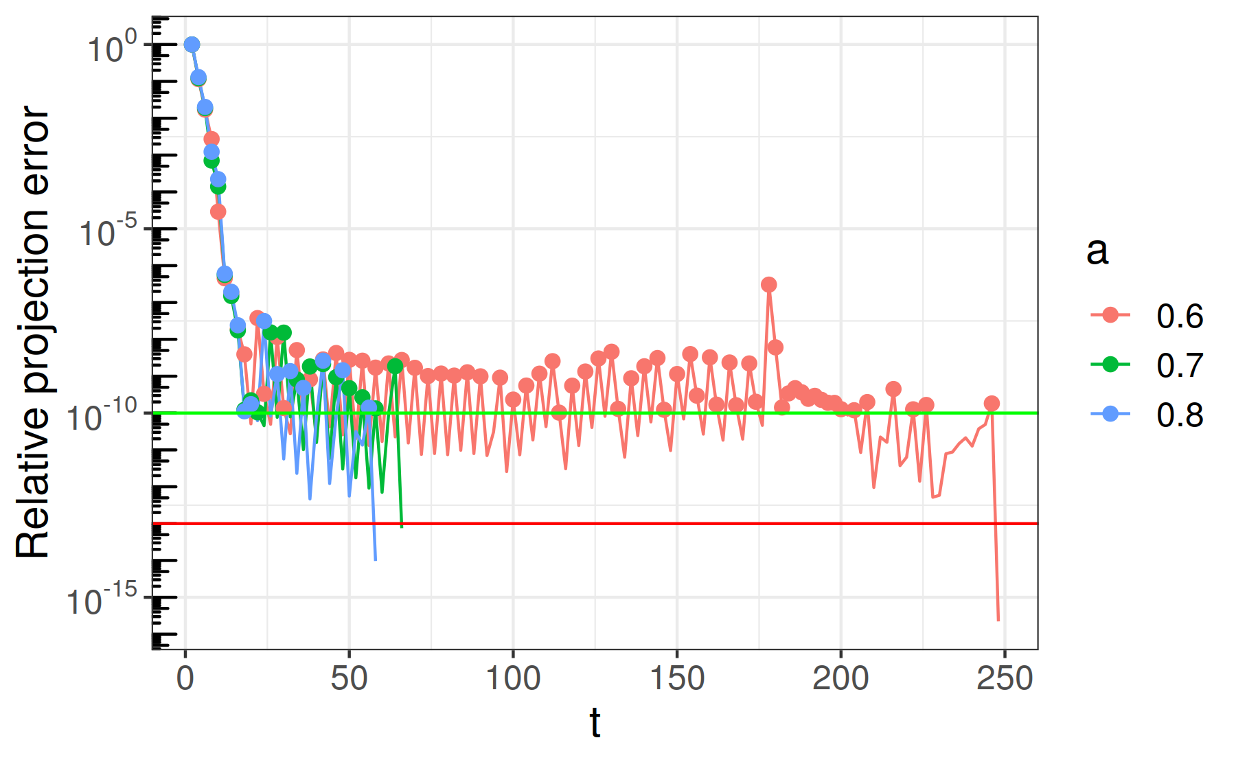
Figure 1: The dependency of the new basis projection error on time. On the vertical axis are the $\left\lVert(I-V_{k-1}V_{k-1}^{T})\hat{V}_{k}\right\rVert_{2}$ values; dots denote the moments when the basis is expanded. The horizontal green line shows the $\varepsilon^{\prime}$ value, the red one — $\varepsilon$.

Figure 1 demonstrates the inner working process of the algorithm during the basis construction for kernel parameter $a$ equal to $0.6$, $0.7$ or $0.8$. We can see that the projection error decreases rapidly at the onset, then oscillates a bit around $\varepsilon^{\prime}$, and eventually crosses the $\varepsilon$ boundary. This, incidentally, highlights another role of the $\varepsilon^{\prime}$ parameter — it effectively prevents the algorithm from over-approximating an initial segment of the solution; we show below the reason why this is important.

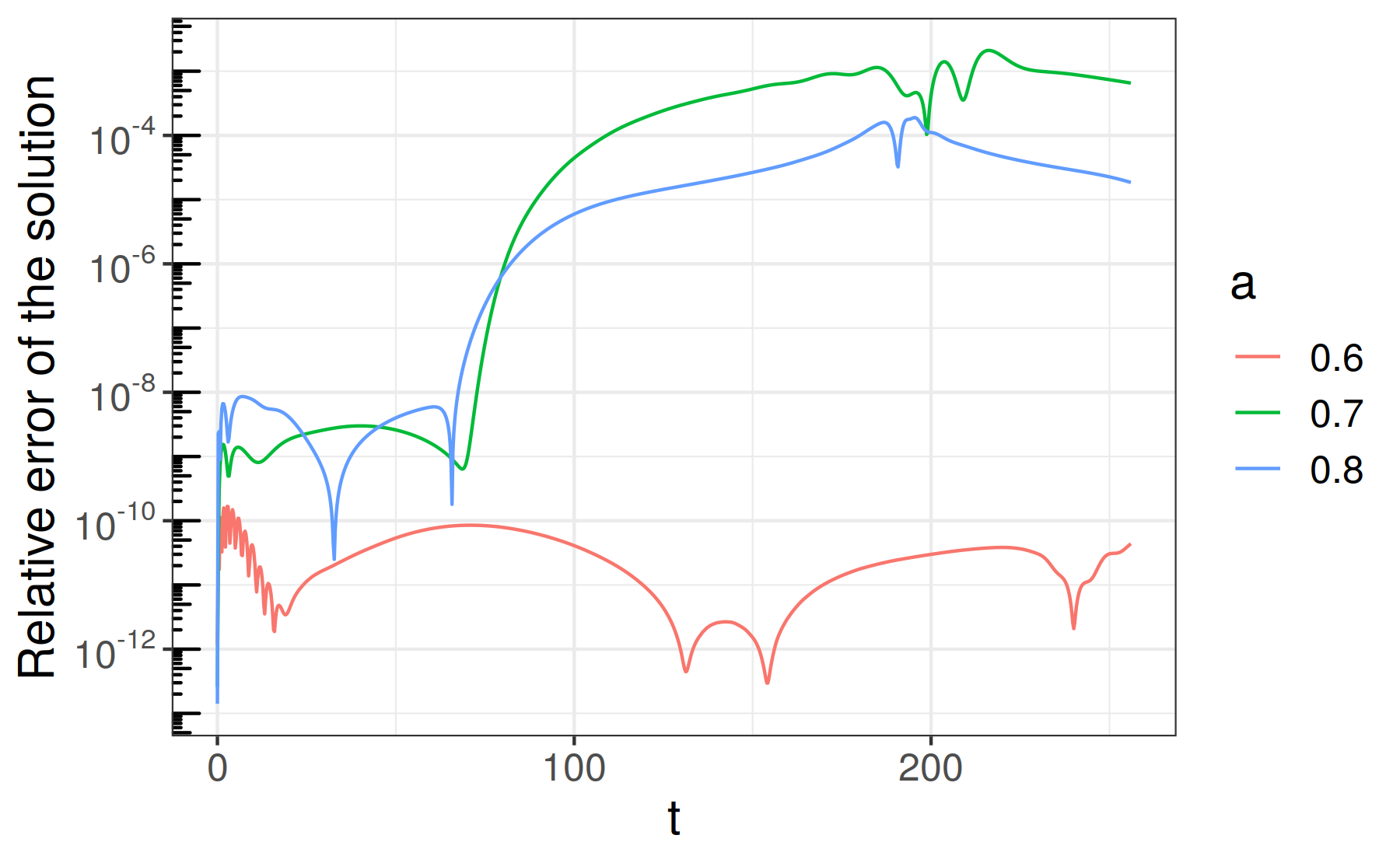
Figure 2: The dependency of the reduced solution relative error in Euclidean norm on time for $N=32768$. On the vertical axis are the values of ${\left\lVert n(t)-\tilde{n}(t)\right\rVert}_{2}/{\left\lVert n(t)\right\rVert}_{2}$, where $\tilde{n}(t)=V\tilde{x}(t)$.

Figure 2 demonstrates an error for a recomputed solution of a reduced system (12) for the time segment $t\in[0,256]$, as compared to a solution of a full system (2). As can be seen from the figure, the error remains small on an interval where the basis was originally constructed, and sharply increases at its end (where the algorithm effectively switches from interpolation to extrapolation) — but, crucially, it still remains bounded around acceptable level $10^{-3}$.

$a$	$t_{\mathrm{full}}$, sec	$t_{\mathrm{red}}$, sec	Basis size
$0.6$	$5.3\times 10^{3}$	$10^{4}$	216
$0.7$	$5.3\times 10^{3}$	$290$	99
$0.8$	$5.3\times 10^{3}$	$61$	86

Table 1: Solution time for $N=32768$. $t_{\mathrm{full}}$ is time to solve the full system (2), $t_{\mathrm{red}}$—time to solve (12).

For the same set of simulations, Table 1 provides the CPU time required to solve full and reduced systems, as well as the eventual size of the basis. As the table clearly demonstrates, the use of the reduction is not always beneficial, especially if fast algorithms for evaluation of the full operator are available; specifically, in the case $a=0.6$, with the basis size of 216, the reduced system is actually more expensive to solve than the full problem.

Since this observation, together with Figure 2, strongly hint at a trade-off between performance and precision, one might be tempted to tweak the $\varepsilon$ parameter to manage it. Unfortunately, as our second set of experiments demonstrates, this is not always straight-forward in practice, which we find rather surprising.

$a$	$\varepsilon$	Reduced solution error	Time span used for basis	Basis size
$0.7$	$10^{-10}$	$3.5\times 10^{-3}$	$[0,100]$	68
$0.7$	$10^{-11}$	$2.3\times 10^{-1}$	$[0,28]$	52
$0.7$	$10^{-12}$	$2.8\times 10^{-5}$	$[0,128]$	101
$0.7$	$10^{-13}$	$2.3\times 10^{-2}$	$[0,68]$	102
$0.7$	$5\times 10^{-14}$	$4.2\times 10^{-3}$	$[0,76]$	112
$0.7$	$10^{-14}$	$4.6\times 10^{-10}$	$[0,256]$	234

Table 2: Solution error as a function of $\varepsilon$ for $N=65536$. Reduced solution error is taken as a maximum relative error in 2-norm over the time span of $[0,256]$.

These experiments are performed with $N=65536$ (we find that the effect is more visible at this dimensionality), with $\delta=\varepsilon$ and $\varepsilon^{\prime}=10^{3}\cdot\varepsilon$. The results are available in Table 2; all the other parameters are the same as in the case above. As can be readily observed, the resulting error does not depend monotonically on $\varepsilon$, and seems to depend more on the actual time span which was used to construct the basis. Note that in the very last row, corresponding to $\varepsilon=10^{-14}$, the algorithm has simply used up the entire time span under evaluation for basis construction, and therefore the error reflects the ‘interpolation’ mode, as seen in Figure 2.

Finally, to test the scalability of our approach, we have tested the algorithm with a larger system with $N=131072$ and $a\in\{0.6,0.7\}$.

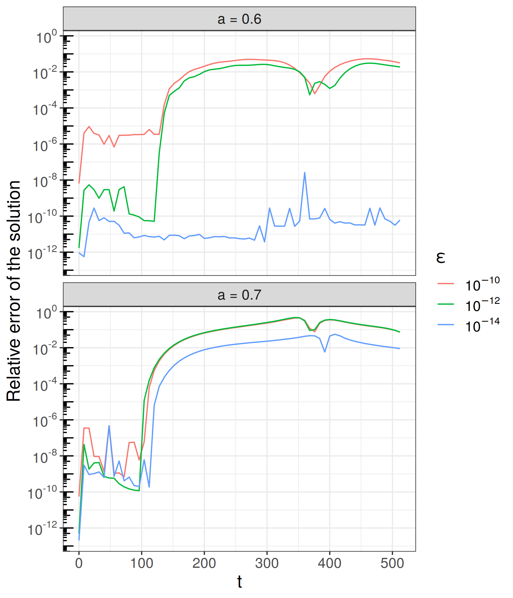
Figure 3: Solution error for $N=131072$, $a=0.7$ and $a=0.6$

$a$	$\varepsilon$	$t_{\mathrm{full}}$, sec	$t_{\mathrm{red}}$, sec	Basis size	Time span used for basis
$0.6$	$10^{-10}$	$8.8\times 10^{4}$	$233.18$	84	$[0,128]$
$0.6$	$10^{-12}$	$8.8\times 10^{4}$	$3.3\times 10^{3}$	115	$[0,124]$
$0.6$	$10^{-14}$	$4.5\times 10^{4}$	$1.2\times 10^{5}$	459	$[0,508]$
$0.7$	$10^{-10}$	$8.8\times 10^{4}$	$144$	70	$[0,106]$
$0.7$	$10^{-12}$	$8.8\times 10^{4}$	$1.3\times 10^{3}$	93	$[0,94]$
$0.7$	$10^{-14}$	$8.8\times 10^{4}$	$6.2\times 10^{3}$	151	$[0,104]$

Table 3: Solution time and basis information for $N=131072$; the test with $a=0.6$ and $\varepsilon=10^{-14}$ was run on a different hardware than the rest.

Figure 3 demonstrates the relative error of the reconstructed solution for $\varepsilon=10^{-10}$, $\varepsilon=10^{-12}$ and $\varepsilon=10^{-14}$, on a longer time segment of $t\in[0,512]$. The same sharp ‘interpolation—extrapolation’ transition is visible here; and results from Table 3 confirm that, in both cases, the ‘interpolation’ region is in the neighbourhood of the transition visible on the graph, except for $a=0.6$, $\varepsilon=10^{-14}$, where almost the entire time span was used for basis construction, and thus there is no visible transition at all.

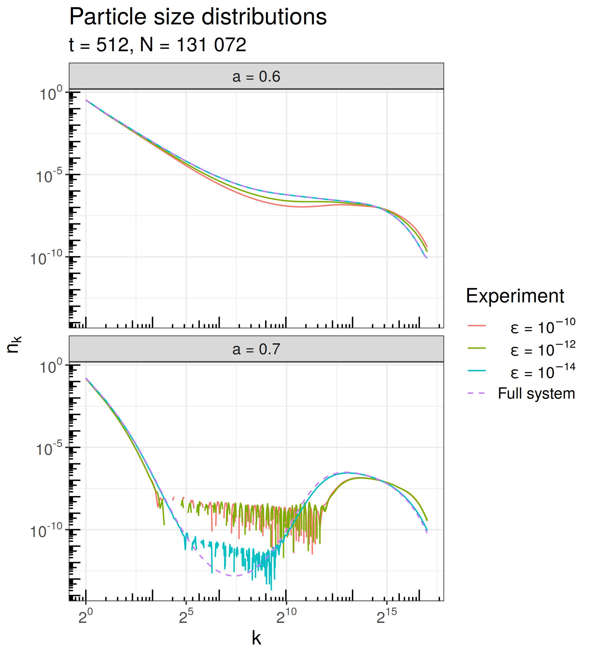
Figure 4: Full particle size distribution (purple line) and reduced solutions (red, green and blue) at $t=512$ for $N=131072$, $a=0.7$ and $a=0.6$. The solution with $\varepsilon=10^{-14}$ is close to the full solution, diverging only for the smallest concentration values

Finally, Figure 4 demonstrates full and reduced solutions at the far end of the simulation time-interval. The solution with $a=0.6$, $\varepsilon=10^{-14}$ is indistinguishable from the precise one, as it is effectively computed in ‘interpolation’ mode, but even the solution with $a=0.7$, $\varepsilon=10^{-14}$ is fairly quantitatively close to the full solution, diverging only for the smallest values concentration of $n_{k}$ — which, surprisingly, do not affect significantly the solution to the either side of their mass range.

Less precise solutions with $\varepsilon=10^{-10}$ and $\varepsilon=10^{-12}$ do not deliver a good quantitative fit (as can already be seen in Figure 3) but, nevertheless, reproduce the qualitative shape of the solution well, despite being significantly cheaper to compute in terms of CPU-time.

6 Conclusion

We have suggested an application of the popular and well-established method of model reduction to the problem of a system of Smoluchowski ODEs, including a candidate method for construction of a reduced basis from an automatically selected prefix of the modelled time span. In our numerical experiments, we demonstrate the existence of such a low-dimensional basis, noticeable speed-ups of computations, and reasonable approximation to the full solution by the reduced model.

At the same time, we also demonstrate problematic sides of the chosen approach — the precision control of the reduced solution seems to be not straight-forward at all due to the nonlinearity of both method and model. Hence, control of accuracy requires more theoretical analysis. In light of these shortcomings, we find our concept very promising for future development in more complicated applied cases and also consider it as fruitful directions of further research.

7 Acknowledgements

We are grateful to Nikolai Zamarashkin for comprehensive discussions during preparation of this work. The work was supported by the Russian Science Foundation, grant 19–11–00338.

References

- [1] M. V. Smoluchowski. Drei vortrage uber diffusion, Brownsche bewegung und koagulation von kolloidteilchen. Zeitschrift fur Physik, 17:557–585, 1916.
- [2] H. Müller. Zur allgemeinen Theorie ser raschen Koagulation. Fortschrittsberichte über Kolloide und Polymere, 27(6):223–250, 1928.
- [3] P. J. Blatz and A. V. Tobolsky. Note on the kinetics of systems manifesting simultaneous polymerization-depolymerization phenomena. The Journal of Physical Chemistry, 49(2):77–80, 1945.
- [4] V. Privman, D. V. Goia, J. Park, and E. Matijevic. Mechanism of Formation of Monodispersed Colloids by Aggregation of Nanosize Precursors. J. Colloid Interface Sci., 213:36–45, 1999.
- [5] Astrid Boje, Jethro Akroyd, and Markus Kraft. A hybrid particle-number and particle model for efficient solution of population balance equations. Journal of Computational Physics, 389:189–218, 2019.
- [6] Astrid Boje, Jethro Akroyd, Stephen Sutcliffe, and Markus Kraft. Study of industrial titania synthesis using a hybrid particle-number and detailed particle model. Chemical Engineering Science, page 115615, 2020.
- [7] N. V. Brilliantov, P. L. Krapivsky, A. Bodrova, F. Spahn, H. Hayakawa, V. Stadnichuk, and J. Schmidt. Size distribution of particles in Saturn’s rings from aggregation and fragmentation. PNAS, 112(31):9536–9541, 2015.
- [8] Larry W Esposito, Nicole Albers, Bonnie K Meinke, Miodrag Sremčević, Prasanna Madhusudhanan, Joshua E Colwell, and Richard G Jerousek. A predator–prey model for moon-triggered clumping in Saturn’s rings. Icarus, 217(1):103–114, 2012.
- [9] Larry W Esposito, Bonnie K Meinke, Joshua E Colwell, Philip D Nicholson, and Matthew M Hedman. Moonlets and clumps in Saturn’s F ring. Icarus, 194(1):278–289, 2008.
- [10] François Leyvraz. Scaling theory and exactly solved models in the kinetics of irreversible aggregation. Physics Reports, 383(2-3):95–212, 2003.
- [11] Kirill Semeniuk and Ashu Dastoor. Current State of Atmospheric Aerosol Thermodynamics and Mass Transfer Modeling: A Review. Atmosphere, 11(2):156, 2020.
- [12] Anwesha Chaudhury, Ivan Oseledets, and Rohit Ramachandran. A computationally efficient technique for the solution of multi-dimensional PBMs of granulation via tensor decomposition. Computers & chemical engineering, 61:234–244, 2014.
- [13] Ivan Timokhin. Tensorisation in the Solution of Smoluchowski Type Equations. In International Conference on Large-Scale Scientific Computing, pages 181–188. Springer, 2019.
- [14] R. Pinnau. Model Reduction via Proper Orthogonal Decomposition. In Schilders W. H. A., van der Vorst H. A., and Rommes J., editors, Model Order Reduction: Theory, Research Aspects and Applications. Mathematics in Industry, volume 13. Springer, Berlin, Heidelberg, 2008.
- [15] Lawrence Sirovich. Turbulence and the Dynamics of Coherent Structures. I–III. Quart. Appl. Math., 45(3):561–590, 1987.
- [16] Anna Shalova and Ivan Oseledets. Deep Representation Learning for Dynamical Systems Modeling. arXiv preprint arXiv:2002.05111, 2020.
- [17] Hisao Hayakawa. Irreversible kinetic coagulations in the presence of a source. Journal of Physics A: Mathematical and General, 20(12):L801, 1987.
- [18] Robin C Ball, Colm Connaughton, Peter P Jones, R Rajesh, and Oleg Zaboronski. Collective oscillations in irreversible coagulation driven by monomer inputs and large-cluster outputs. Physical review letters, 109(16):168304, 2012.
- [19] S. A. Matveev, V. I. Stadnichuk, E. E. Tyrtyshnikov, A. P. Smirnov, N. V. Ampilogova, and N. V. Brilliantov. Anderson acceleration method of finding steady-state particle size distribution for a wide class of aggregation–fragmentation models. Computer Physics Communications, 224:154–163, 2018.
- [20] IV Timokhin, SA Matveev, N Siddharth, Eugene E Tyrtyshnikov, AP Smirnov, and Nikolai V Brilliantov. Newton method for stationary and quasi-stationary problems for smoluchowski-type equations. Journal of Computational Physics, 382:124–137, 2019.
- [21] PL Krapivsky and Colm Connaughton. Driven brownian coagulation of polymers. The Journal of chemical physics, 136(20):204901, 2012.
- [22] SA Matveev, AA Sorokin, AP Smirnov, and EE Tyrtyshnikov. Oscillating stationary distributions of nanoclusters in an open system. Mathematical and Computer Modelling of Dynamical Systems, pages 1–14, 2020.
- [23] N. V. Brilliantov, W. Otieno, S. A. Matveev, A. P. Smirnov, E. E. Tyrtyshnikov, and P. L. Krapivsky. Steady oscillations in aggregation-fragmentation processes. PHYSICAL REVIEW E, 98(1), 2018.
- [24] Jonasz Słomka and Roman Stocker. Bursts characterize coagulation of rods in a quiescent fluid. Physical Review Letters, 124(25):258001, 2020.
- [25] Robert L Pego and Juan JL Velázquez. Temporal oscillations in becker–döring equations with atomization. Nonlinearity, 33(4):1812, 2020.
- [26] S. A. Matveev, A. P. Smirnov, and E. E. Tyrtyshnikov. A fast numerical method for the Cauchy problem for the Smoluchowski equation. Journal of Computational Physics, 282(FEB):23–32, 2015.