Non-Mergeable Sketching for Cardinality Estimation

Abstract

Cardinality estimation is perhaps the simplest non-trivial statistical problem that can be solved via sketching. Industrially-deployed sketches like HyperLogLog, MinHash, and PCSA are mergeable, which means that large data sets can be sketched in a distributed environment, and then merged into a single sketch of the whole data set. In the last decade a variety of sketches have been developed that are non-mergeable, but attractive for other reasons. They are simpler, their cardinality estimates are strictly unbiased, and they have substantially lower variance.

We evaluate sketching schemes on a reasonably level playing field, in terms of their memory-variance product (MVP). I.e., a sketch that occupies $5m$ bits and whose relative variance is $2/m$ (standard error $\sqrt{2/m}$) has an MVP of $10$. Our contributions are as follows.

• Cohen [14] and Ting [34] independently discovered what we call the Martingale transform for converting a mergeable sketch into a non-mergeable sketch. We present a simpler way to analyze the limiting MVP of Martingale-type sketches.

• Pettie and Wang proved that the Fishmonger sketch [31] has the best MVP, $H_{0}/I_{0}\approx 1.98$, among a class of mergeable sketches called “linearizable” sketches. ($H_{0}$ and $I_{0}$ are precisely defined constants.) We prove that the Martingale transform is optimal in the non-mergeable world, and that Martingale Fishmonger in particular is optimal among linearizable sketches, with an MVP of $H_{0}/2\approx 1.63$. E.g., this is circumstantial evidence that to achieve 1% standard error, we cannot do better than a 2 kilobyte sketch.

• Martingale Fishmonger is neither simple nor practical. We develop a new mergeable sketch called Curtain that strikes a nice balance between simplicity and efficiency, and prove that Martingale Curtain has limiting $\textsf{MVP}\approx 2.31$. It can be updated with $O(1)$ memory accesses and it has lower empirical variance than Martingale LogLog, a practical non-mergeable version of HyperLogLog.

1 Introduction

Cardinality estimation is a fundamental problem in streaming and sketching with diverse applications in databases [12, 21], network monitoring [5, 8, 37, 11], nearest neighbor search [32], caching [35], and genomics [30, 17, 36, 2]. In the sequential setting of this problem, we receive the elements of a multiset $\mathscr{A}=\{a_{1},a_{2},\ldots,a_{N}\}$ one at a time. We maintain a small sketch $S$ of the elements seen so far, such that the true cardinality $\lambda=|\mathscr{A}|$ is estimated by some $\hat{\lambda}(S)$. The distributed setting is similar, except that $\mathscr{A}$ is partitioned arbitrarily among several machines, the shares being sketched separately and combined into a sketch of $\mathscr{A}$. Only mergeable sketches are deployed in distributed settings; see Definition 2 below.

Definition 1.

In the random oracle model $\mathscr{A}\subseteq[U]$ and we have oracle access to a uniformly random permutation $h:[U]\rightarrow[U]$ (or a uniformly random hash function $h:[U]\rightarrow[0,1]$). In the standard model we can generate random bits as necessary, but must explicitly store any hash functions in the sketch.

Definition 2.

Suppose $\mathscr{A}^{(1)},\mathscr{A}^{(2)}$ are multisets such that $\mathscr{A}=\mathscr{A}^{(1)}\cup\mathscr{A}^{(2)}$. A sketching scheme is mergeable if, whenever, $\mathscr{A}^{(1)},\mathscr{A}^{(2)}$ are sketched as $S^{(1)},S^{(2)}$ (using the same random oracle $h$ or the same source of random bits in the standard model), the sketch $S$ of $\mathcal{A}$ can be computed from $S^{(1)},S^{(2)}$ alone.

Standard model sketches [1, 3, 4, 6, 22, 27] usually make an $(\epsilon,\delta)$-guarantee, i.e.,

$$\Pr\left(\hat{\lambda}\not\in[(1-\epsilon)\lambda,(1+\epsilon)\lambda]\right)<\delta.$$

The state-of-the-art standard model sketch [6, 27] uses $O(\epsilon^{-2}\log\delta^{-1}+\log U)$ bits, which is optimal at this level of specificity, as it meets the space lower bounds of $\Omega(\log U)$, $\Omega(\epsilon^{-2})$ (when $\delta=\Theta(1)$), and $\Omega(\epsilon^{-2}\log\delta^{-1})$ [1, 25, 26]. However, the leading constants hidden by [6, 27] are quite large.

In the random oracle model the cardinality estimate $\hat{\lambda}$ typically has negligible bias, and errors are expressed in terms of the relative variance $\lambda^{-2}\cdot\operatorname{Var}(\hat{\lambda}\mid\lambda)$ or relative standard deviation $\lambda^{-1}\sqrt{\operatorname{Var}(\hat{\lambda}\mid\lambda)}$, also called the standard error. Sketches that use $\Omega(m)$ bits typically have relative variances of $O(m)$. Thus, the most natural way to measure the quality of the sketching scheme itself is to look at its limiting memory-variance product (MVP), i.e., the product of its memory and variance as $m\rightarrow\infty$.

Until about a decade ago, all standard/random oracle sketches were mergeable, and suitable to both distributed and sequential applications. For reasons that are not clear to us, the idea of non-mergeable sketching was discovered independently by multiple groups [10, 24, 14, 34] at about the same time, and quite late in the 40-year history of cardinality estimation. Chen, Cao, Shepp, and Nguyen [10] invented the S-Bitmap in 2011, followed by Helmi, Lumbroso, Martínez, and Viola’s[24] Recordinality in 2012. In 2014 Cohen [14] and Ting [34] independently invented what we call the Martingale transform, which is a simple, mechanical way to transform any mergeable sketch into a (better) non-mergeable sketch.

In a companion paper [31], we analyzed the MVPs of mergeable sketches under the assumption that the sketch was compressed to its entropy bound. Fishmonger (an entropy compressed variant of PCSA with a different estimator function) was shown to have $\textsf{MVP}=H_{0}/I_{0}\approx 1.98$, where

$$H_{0} =(\ln 2)^{-1}+\sum_{k=1}^{\infty}k^{-1}\log_{2}(1+1/k) \mbox{ and \ }I_{0} =\zeta(2)=\pi^{2}/6.$$

Furthermore, $H_{0}/I_{0}$ was shown to be the minimum MVP among linearizable sketches, a subset of mergeable sketches that includes all the popular sketches (HyperLogLog, PCSA, MinHash, etc.).

Our aim in this paper is to build a useful framework for designing and analyzing non-mergeable sketching schemes, and, following [31], to develop a theory of space-variance optimality in the non-mergeable world. We work in the random oracle model. Our results are as follows.

• Although the Martingale transform itself is simple, analyzing the variance of these sketches is not. For example, Cohen [14] and Ting [34] estimated the standard error of Martingale LogLog to be about $\approx\sqrt{3/(4m)}\approx 0.866/\sqrt{m}$ and about $\approx 1/(2\alpha_{m}m)$, respectively, where the latter tends to $\sqrt{\ln 2/m}\approx 0.8326/\sqrt{m}$ as $m\rightarrow\infty$. We give a general method for determining the limiting relative variance of Martingale sketches that is strongly influenced by Ting’s perspective.

• What is the most efficient (smallest MVP) non-mergeable sketch for cardinality estimation? The best Martingale sketches perform better than the ad hoc non-mergeable S-Bitmap and Recordinality, but perhaps there is a completely different, better way to systematically build non-mergeable sketches. We prove that up to some natural assumptions the best non-mergeable sketch is a Martingale X sketch, for some X. Furthermore, we prove that Martingale Fishmonger, having MVP of $H_{0}/2\approx 1.63$, is optimal among all Martingale X sketches, where X is linearizable. This provides some circumstantial evidence that Martingale Fishmonger is optimal, and that if we want, say, 1% standard error, we need to use a $H_{0}/2\cdot(0.01)^{-2}$-bit sketch, $\approx$ 2 kilobytes.

• Martingale Fishmonger has an attractive MVP, but it is slow and cumbersome to implement. We propose a new mergeable sketch called Curtain that is “naturally” space efficient and easy to update in $O(1)$ memory accesses, and prove that Martingale Curtain has a limiting $\textsf{MVP}\approx 2.31$.

1.1 Prior Work: Mergeable Sketches

Let $S_{i}$ be the state of the sketch after processing $(a_{1},\ldots,a_{i})$.

The state of the PCSA sketch [20] is a 2D matrix $S\in\{0,1\}^{m\times\log U}$ and the hash function $h:[U]\rightarrow[m]\times\mathbb{Z}^{+}$ produces two indices: $h(a)=(j,k)$ with probability $m^{-1}2^{-k}$. $S_{i}(j,k)=1$ iff $\exists i^{\prime}\in[i].h(a_{i^{\prime}})=(j,k)$. Flajolet and Martin [20] proved that a certain estimator has standard error $0.78/\sqrt{m}$, making the MVP around $(0.78)^{2}\log U\approx 0.6\log U$.

Durand and Flajolet’s LogLog sketch [16] consists of $m$ counters. It interprets $h$ exactly as in PCSA, and sets $S_{i}(j)=k$ iff $k$ is maximum such that $\exists i^{\prime}\in[i].h(a_{i^{\prime}})=(j,k)$. Durand and Flajolet’s estimator is of the form $\hat{\lambda}(S)\propto m2^{m^{-1}\sum_{j}S(j)}$ and has standard error $\approx 1.3/\sqrt{m}$. Flajolet, Fusy, Gandouet, and Meunier’s HyperLogLog [19] is the same sketch but with the estimator $\hat{\lambda}(S)\propto m^{2}(\sum_{j}2^{-S(j)})^{-1}$. They proved that it has standard error tending to $\approx 1.04/\sqrt{m}$. As the space is $m\log\log U$ bits, the MVP is $\approx 1.08\log\log U$.

The MinCount sketch (aka MinHash or Bottom-$m$ [13, 15, 7]) stores the smallest $m$ hash values, which we assume requires $\log U$ bits each. Using an appropriate estimator [23, 9, 29], the standard error is $1/\sqrt{m}$ and $\textsf{MVP}{}=\log U$.

It is straightforward to see that the entropy of PCSA and LogLog are both $\Theta(m)$. Scheuermann and Mauve [33] experimented with entropy compressed versions of PCSA and HyperLogLog and found PCSA to be slightly superior. Rather than use the given estimators of [20, 19, 16], Lang [28] used Maximum Likelihood-type Estimators and found entropy-compressed PCSA to be significantly better than entropy-compressed LogLog (with MLE estimators). Pettie and Wang [31] defined the Fisher-Shannon ($\mathsf{Fish}$) number of a sketch as the ratio of its Shannon entropy (controlling its entropy-compressed size) to its Fisher information (controlling the variance of a statistically efficient estimator), and proved that the $\mathsf{Fish}$-number of any base-$q$ PCSA is $H_{0}/I_{0}$, and that the $\mathsf{Fish}$-number of base-$q$ LogLog is worse, but tends to $H_{0}/I_{0}$ in the limit as $q\rightarrow\infty$. Here $H_{0}$ and $I_{0}$ are:

$$H_{0} =(\ln 2)^{-1}+\sum_{k=1}^{\infty}k^{-1}\log_{2}(1+1/k)$$

$$\mbox{ and \ }I_{0} =\zeta(2)=\pi^{2}/6.$$

Mergeable Sketch	Limiting MVP	Notes
PCSA [20]	$.6\log U\approx 38.9$	For $U=2^{64}$
LogLog [16]	$1.69\log\log U\approx 10.11$	For $U=2^{64}$
MinCount [23, 9, 29]	$\log U=64$	For $U=2^{64}$
HyperLogLog [19]	$1.08\log\log U\approx 6.48$	For $U=2^{64}$
Fishmonger [31]	$H_{0}/I_{0}\approx 1.98$
Non-Mergeable Sketch
S-Bitmap [10]	$O(\log^{2}(U/m))$
Recordinality [24]	$O(\log(\lambda/m)\log U)$
Martingale PCSA new	$0.35\log U\approx 22.4$	For $U=2^{64}$
Martingale LogLog [14, 34]	$0.69\log\log U\approx 4.16$	For $U=2^{64}$
Martingale MinCount [14, 34]	$0.5\log U=32$	For $U=2^{64}$
Martingale Fishmonger new	$H_{0}/2\approx 1.63$	$H_{0}=(\ln 2)^{-1}+\sum_{k\geq 1}\frac{\log_{2}(1+1/k)}{k}$
Martingale Curtain new	$\approx 2.31$	Theorem 1 with $(q,a,h)=(2.91,2,1)$
Non-Mergeable Lower Bound
Martingale X new	$\geq H_{0}/2$	X is a linearizable sketch

Table 1: A selection of results on composable sketches (top) and non-composable Martingale sketches (bottom) in terms of their limiting memory-variance product (MVP). Logarithms are base 2.

1.2 Prior Work: Non-Mergeable Sketches

Chen, Cao, Shepp, and Nguyen’s S-Bitmap [10] consists of a bit string $S\in\{0,1\}^{m}$ and $m$ known constants $0\leq\tau_{0}<\tau_{1}<\cdots<\tau_{m-1}<1$. It interprets $h(a)=(j,\rho)\in[m]\times[0,1]$ as an index $j$ and real $\rho$ and when processing $a$, sets $S(j)\leftarrow 1$ iff $\rho>\tau_{\operatorname{HammingWeight}(S)}$. One may confirm that $S$ is insensitive to duplicates in the stream $\mathcal{A}$, but its state depends on the order in which $\mathcal{A}$ is scanned. By setting the $\tau$-thresholds and estimator properly, the standard error is $\approx\ln(eU/m)/(2\sqrt{m})$ and $\textsf{MVP}=O(\log^{2}(U/m))$.

Recordinality [24] is based on MinCount; it stores $(S,\operatorname{cnt})$, where $S$ is the $m$ smallest hash values encountered and $\operatorname{cnt}$ is the number of times that $S$ has changed. The estimator looks only at $\operatorname{cnt}$, not $S$, and has standard error $\approx\sqrt{\ln(\lambda/em)/m}$ and $\textsf{MVP}{}=O(\log(\lambda/m)\log U)$.

Cohen [14] and Ting [34] independently described how to turn any sketch into a non-mergeable sketch using what we call the Martingale transform. Let $S_{i}$ be the state of the original sketch after seeing $(a_{1},\ldots,a_{i})$ and $P_{i+1}=\Pr(S_{i+1}\neq S_{i}\mid S_{i},a_{i+1}\not\in\{a_{1},\ldots,a_{i}\})$ be the probability that it changes state upon seeing a new element $a_{i+1}$. The state of the Martingale sketch is $(S_{i},\hat{\lambda}_{i})$. Upon processing $a_{i+1}$ it becomes $(S_{i+1},\hat{\lambda}_{i+1})$, where

$$\hat{\lambda}_{i+1}=\hat{\lambda}_{i}+P_{i+1}^{-1}\cdot\left\llbracket\rule[-2.84526pt]{0.0pt}{2.84526pt}\rule{0.0pt}{9.95845pt}S_{i+1}\neq S_{i}\right\rrbracket.$$

Here $\left\llbracket\rule[-2.84526pt]{0.0pt}{2.84526pt}\rule{0.0pt}{9.95845pt}\mathcal{E}\right\rrbracket$ is the indicator variable for the event $\mathcal{E}$. We assume the original sketch is insensitive to duplicates, so

$$\mathbb{E}(\hat{\lambda}_{i+1})=\left\{\begin{array}[]{l@{\hspace*{1cm}}l}\hat{\lambda}_{i}\hfil\hskip 28.45274pt&\mbox{when $a_{i+1}\in\{a_{1},\ldots,a_{i}\}$ (and hence $S_{i+1}=S_{i}$)}\\ \hat{\lambda}_{i}+1\hfil\hskip 28.45274pt&\mbox{when $a_{i+1}\not\in\{a_{1},\ldots,a_{i}\}$.}\end{array}\right.$$

Thus, with $\hat{\lambda}_{0}=\lambda_{0}=0$, $\hat{\lambda}_{i}$ is an unbiased estimator of the true cardinality $\lambda_{i}=|\{a_{1},\ldots,a_{i}\}|$ and $(\hat{\lambda}_{i}-\lambda_{i})_{i}$ is a martingale. The Martingale-transformed sketch requires the same space, plus just $\log U$ bits to store the estimate $\hat{\lambda}$.

Cohen and Ting [14, 34] both proved that Martingale MinCount has standard error $1/(2\sqrt{m})$ and $\textsf{MVP}=(\log U)/2$. They gave different estimates for the standard error of Martingale LogLog. Ting’s estimate is quite accurate, and tends to $\sqrt{\ln 2/m}$ as $m\rightarrow\infty$, giving it an $\textsf{MVP}=\ln 2\log\log U\approx 0.69\log\log U$.

1.3 The Dartboard Model

The dartboard model [31] is useful for describing cardinality sketches with a single, uniform language. The dartboard model is essentially the same as Ting’s [34] area cutting process, but with a specific, discrete cell partition and state space fixed in advance.

The dartboard is the unit square $[0,1]^{2}$, partitioned into a set $\mathscr{C}=\{c_{0},\ldots,c_{|\mathscr{C}|-1}\}$ of cells of various sizes. Every cell may be either occupied or unoccupied; the state is the set of occupied cells and the state space some $\mathscr{S}\subseteq 2^{\mathscr{C}}$.

We process a stream of elements one by one; when a new element is encountered we throw a dart uniformly at random at the dartboard and update the state in response. The relationship between the state and the dart distribution satisfies two rules:

(R1)

Every cell with at least one dart is occupied; occupied cells may contain no darts.

(R2)

If a dart lands in an occupied cell, the state does not change.

As a consequence of (R1) and (R2), if a dart lands in an empty cell the state must change, and occupied cells may never become unoccupied. Dart throwing is merely an intuitive way of visualizing the hash function. Base-$q$ PCSA and LogLog use the same cell partition but with different state spaces; see Figure 1.

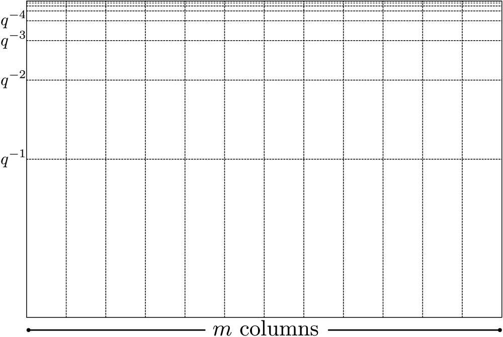
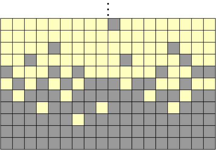
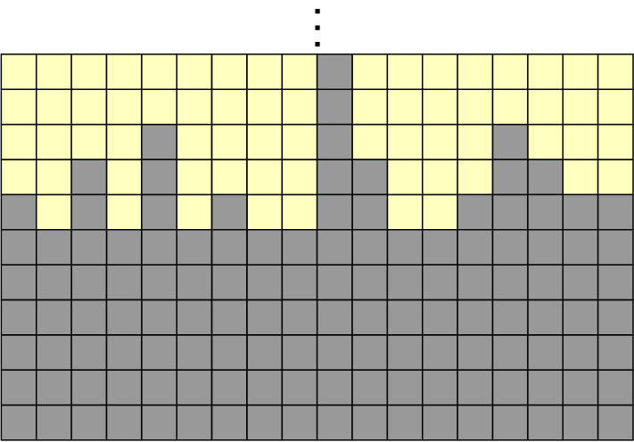
(a)	(b)	(c)

Figure 1: The unit square is partitioned into $m$ columns. Each column is partitioned into cells. Cell $j$ covers the vertical interval $[q^{-(j+1)},q^{-j})$. (b) The state of a PCSA sketch records precisely which cells contain a dart (gray); all others are empty (yellow). (c) The state of the corresponding LogLog sketch.

It was observed [31] that the dartboard model includes all mergeable sketches, and some non-mergeable ones like S-Bitmap. Recordinality and the Martingale sketches obey rules (R1),(R2) but are not strictly dartboard sketches as they maintain some small state information ($\operatorname{cnt}$ or $\hat{\lambda}$) outside of the set of occupied cells. Nonetheless, it is useful to speak of the dartboard part of their state information.

1.4 Linearizable Sketches

The lower bound of [31] applies to linearizable sketches, a subset of mergeable sketches. A sketch is called linearizable if it is possible to encode the occupied/unoccupied status of its cells in some fixed linear order $(c_{0},\ldots,c_{\mathscr{C}-1})$, so whether $c_{i}$ is occupied only depends on the status of $c_{0},\ldots,c_{i-1}$ and whether $c_{i}$ has been hit by a dart. (Thus, it is independent of $c_{i+1},\ldots,c_{\mathscr{C}-1}$.) Specifically, let $Y_{i},Z_{i}$ be the indicators for whether $c_{i}$ is occupied, and has been hit by a dart, respectively, and $\mathbf{Y}_{i}=(Y_{0},\ldots,Y_{i})$. The state of the sketch is $\mathbf{Y}_{\mathscr{C}-1}$; it is called linearizable if there is some monotone function $\phi:\{0,1\}^{*}\rightarrow\{0,1\}$ such that

$$Y_{i}=Z_{i}\vee\phi(\mathbf{Y}_{i-1}).$$

I.e., if $\phi(\mathbf{Y}_{i-1})=1$, $c_{i}$ is forced to be occupied and the state is forever independent of $Z_{i}$.

PCSA-type sketches [20, 18] are linearizable, as are (Hyper)LogLog [19, 16], and all MinCount, MinHash, and Bottom-$m$ type sketches [13, 7, 23, 9, 29]. It is very easy to engineer non-linearizable sketches; see [31]. The open problem is whether this is ever a good idea in terms of memory-variance performance.

1.5 Organization

In Section 2 we introduce the Curtain sketch, which is a linearizable (hence mergeable) sketch in the dartboard model. In Section 3 we prove some general theorems on the bias and asymptotic relative variance of Martingale-type sketches, and in Section 4 we apply this framework to bound the limiting MVP of Martingale PCSA, Martingale Fishmonger, and Martingale Curtain.

In Section 5 we prove some results on the optimality of the Martingale transform itself, and that Martingale Fishmonger has the lowest variance among those based on linearizable sketches.

Section 6 presents some experimental findings that demonstrate that the conclusions drawn from the asymptotic analysis of Martingale sketches are extremely accurate in the pre-asymptotic regime as well, and that Martingale Curtain has lower variance than Martingale LogLog.

2 The Curtain Sketch

Design Philosophy.

Our goal is to strike a nice balance between the simplicity and time-efficiency of (Hyper)LogLog, and the superior information-theoretic efficiency of PCSA, which can only be fully realized under extreme (and time-inefficient) compression to its entropy bound [31, 28]. Informally, if we are dedicating at least 1 bit to encode the status of a cell, the best cells to encode have mass $\Theta(\lambda^{-1})$ and we should design a sketch that maximizes the number of such cells encoded.

We assume the dartboard is partitioned into $m$ columns; define $\operatorname{Cell}(j,i)$ to be the cell in column $i$ covering the vertical interval $[q^{-(j+1)},q^{-j})$. In a PCSA sketch, the occupied cells are precisely those with at least one dart. In LogLog, the occupied cells in each column are contiguous, extending to the highest cell containing a dart. In Figure 1, cells are drawn with uniform sizes for clarity.

Consider the vector $v=(g_{0},g_{1},\ldots,g_{m-1})$ where $\operatorname{Cell}(g_{i},i)$ is the highest occupied cell in LogLog/PCSA. The curtain of $v$ w.r.t. allowable offsets $\mathscr{O}$ is a vector $v_{\operatorname{curt}}=(\hat{g}_{0},\hat{g}_{1},\ldots,\hat{g}_{m-1})$ such that (i) $\forall i\in[1,m-1].\,\hat{g}_{i}-\hat{g}_{i-1}\in\mathscr{O}$, and (ii) $v_{\operatorname{curt}}$ is the minimal such vector dominating $v$, i.e., $\forall i.\,\hat{g}_{i}\geq g_{i}$. Although we have described $v_{\operatorname{curt}}$ as a function of $v$, it is clearly possible to maintain $v_{\operatorname{curt}}$ as darts are thrown, without knowing $v$.

We have an interest in $|\mathscr{O}|$ being a power of 2 so that curtain vectors may be encoded efficiently, as a series of offsets. On the other hand, it is most efficient if $\mathscr{O}$ is symmetric around zero. For these reasons, we use a base-$q$ “sawtooth” cell partition of the dartboard; see Figure 2. Henceforth $\operatorname{Cell}(j,i)$ is defined as usual, except $j$ is an integer when $i$ is even and a half-integer when $i$ is odd. Then the allowable offsets are $\mathscr{O}_{a}=\{-(a-1/2),-(a-3/2),\ldots,-1/2,1/2,\ldots,a-3/2,a-1/2\}$, for some $a$ that is a power of 2.

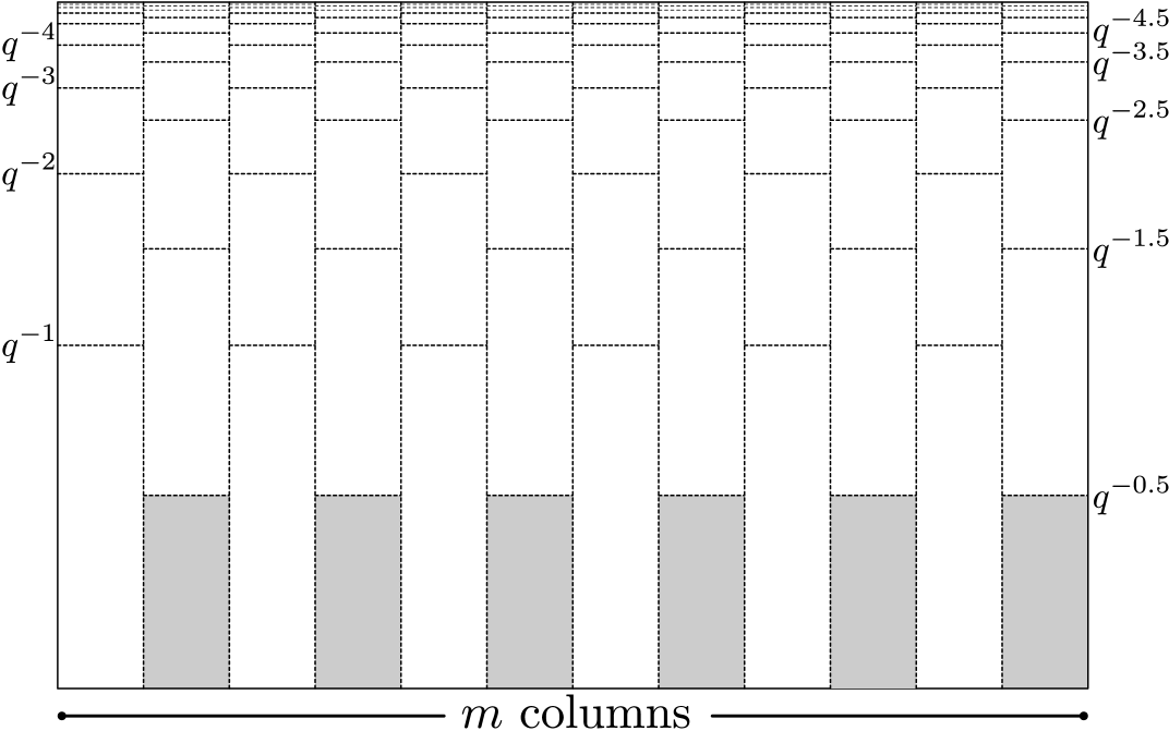
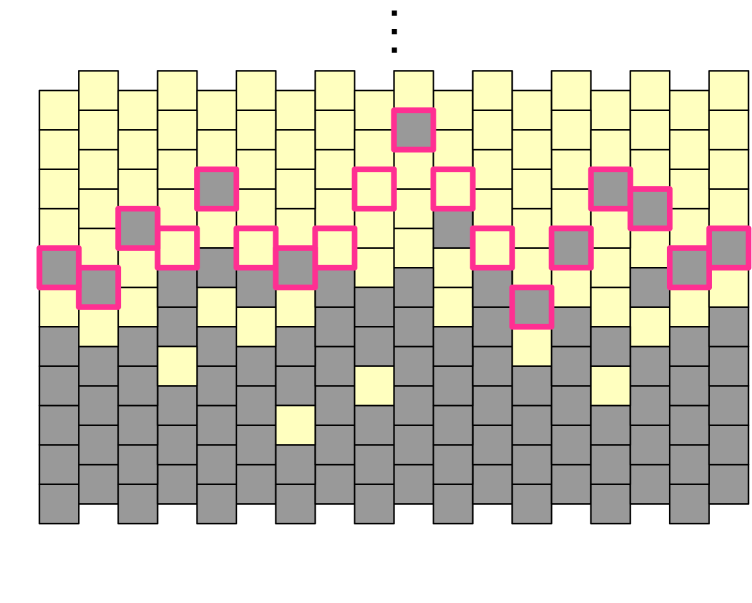
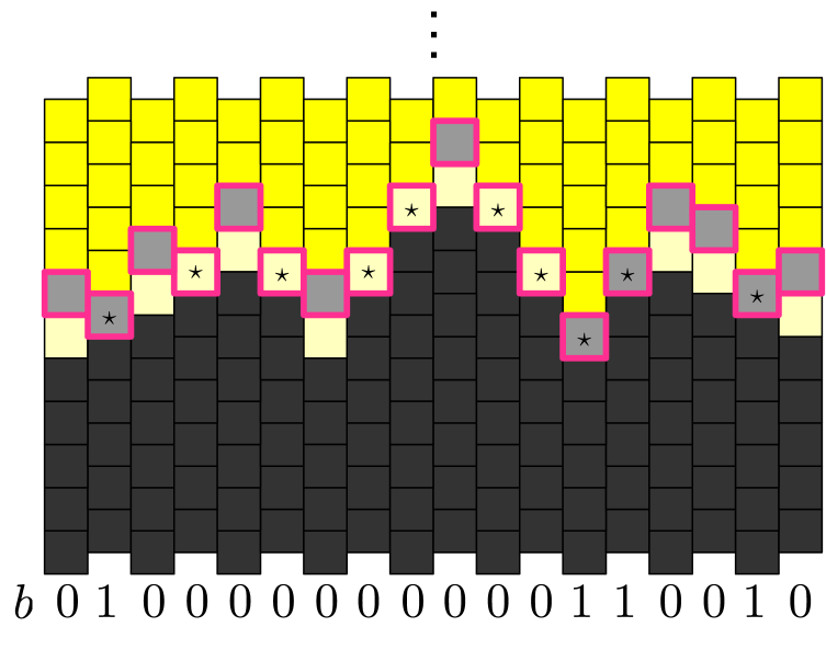
(a)	(b)	(c)

Figure 2: (a) The base-$q$ “sawtooth” cell partition. (b) and (c) depict a Curtain sketch w.r.t. $\mathscr{O}=\{-3/2,-1/2,1/2,3/2\}$ and $h=1$. (b) Gray cells contain at least one dart; light yellow cells contain none. The curtain $v_{\operatorname{curt}}=(\hat{g}_{i})$ is highlighted with a pink boundary. (c) Columns that are in tension have a $\star$ in their curtain cell. All dark gray cells are occupied and all dark yellow cells are free according to Rule 3. All other cells are occupied/free (light gray, light yellow) according to Rules 1 and 2.

Let $\operatorname{Cell}(g_{i},i)$ is the highest cell containing a dart in column $i$ in the sawtooth cell partition and $v_{\operatorname{curt}}=(\hat{g}_{i})$ be the curtain vector of $v=(g_{i})$ w.r.t. offsets $\mathscr{O}=\mathscr{O}_{a}$. We say column $i$ is in tension if $(\cdots,\hat{g}_{i-1},\hat{g}_{i}-1,\hat{g}_{i+1},\cdots)$ is not a valid curtain, i.e., if $\hat{g}_{i}-\hat{g}_{i-1}=\min(\mathscr{O})$ or $\hat{g}_{i+1}-\hat{g}_{i}=\max(\mathscr{O})$. In particular, if column $i$ is not in tension, then $\operatorname{Cell}(\hat{g}_{i},i)$ must contain at least one dart, for if it contained no darts the curtain would be dropped to $\hat{g}_{i}-1$ at column $i$. However, if column $i$ is in tension, then $\operatorname{Cell}(\hat{g}_{i},i)$ might not contain a dart.

The Curtain sketch encodes $v_{\operatorname{curt}}=(\hat{g}_{i})$ w.r.t. the base-$q$ sawtooth cell partition and offsets $\mathscr{O}_{a}$, and a bit-array $b=\{0,1\}^{h\times m}$. This sketch designates each cell occupied or free as follows.

Rule 1.

If column $i$ is not in tension then $\operatorname{Cell}(\hat{g}_{i},i)$ is occupied, and $b(\cdot,i)$ encodes the status of the $h$ cells below the curtain, i.e., $\operatorname{Cell}(\hat{g}_{i}-(j+1),i)$ is occupied iff $b(j,i)=1$, $j\in\{0,\ldots,h-1\}$.

Rule 2.

If column $i$ is in tension, then $\operatorname{Cell}(\hat{g}_{i}-j,i)$ is occupied iff $b(j,i)=1$, $j\in\{0,\ldots,h-1\}$.

Rule 3.

Every cell above the curtain is free ($\operatorname{Cell}(\hat{g}_{i}+j,i)$, when $j\geq 1$) and all remaining cells are occupied.

Figure 2 gives an example of a Curtain sketch, with $\mathscr{O}=\{-3/2,-1/2,1/2,3/2\}$ and $h=1$. (The base $q$ of the cell partition is unspecified in this example.)

Theorem 1.

Consider the Martingale Curtain sketch with parameters $q,a,h$ (base $q$, $\mathscr{O}_{a}=\{-(a-1/2),\ldots,a-1/2\}$, and $b\in\{0,1\}^{h\times m}$), and let $\hat{\lambda}$ be its estimate of the true cardinality $\lambda$.

1. $\hat{\lambda}$ is an unbiased estimate of $\lambda$.

2. The relative variance of $\hat{\lambda}$ is:

   $$\frac{1}{\lambda^{2}}\operatorname{Var}(\hat{\lambda}\mid\lambda)=\frac{(1+o_{\lambda/m}(1)+o_{m}(1))q\ln q}{2m(q-1)}\left(\frac{q-1}{q}+\frac{2}{q^{h}(q^{a-1/2}-1)}+\frac{1}{q^{h+1}}\right),$$

   As a result, the limiting MVP of Martingale Curtain is

   $$\textsf{MVP}=(\log_{2}(2a)+h)\times\frac{q\ln q}{2(q-1)}\left(\frac{q-1}{q}+\frac{2}{q^{h}(q^{a-1/2}-1)}+\frac{1}{q^{h+1}}\right).$$

Proof.

Follows from Theorems 3 and 6. ∎

Here $o_{\lambda/m}(1)$ and $o_{m}(1)$ are terms that go to zero as $m$ and $\lambda/m$ get large. Recall that for practical reasons we want to parameterize Theorem 1 with $a$ a power of 2 and $h$ an integer, but it is realistic to set $q>1$ to be any real. Given these constraints, the optimal setting is $q=2.91$, $a=2$, and $h=1$, exactly as in the example in Figure 2. This uses $\log\log U+3(m-1)$ bits to store the sketch proper, $\log U$ bits to store $\hat{\lambda}$, and achieves a limiting $\textsf{MVP}\approx 2.31$. In other words, to achieve a standard error $1/\sqrt{b}$, we need about $2.31b$ bits.

Implementation Considerations.

We encode a curtain $(\hat{g}_{0},\hat{g}_{1},\ldots,\hat{g}_{m-1})$ as $\hat{g}_{0}$ and an offset vector $(o_{1},o_{2},\ldots,o_{m-1})$, $o_{i}=\hat{g}_{i}-\hat{g}_{i-1}$, where $\hat{g}_{0}$ takes $\log_{2}\log_{q}U\leq 6$ bits and $o_{i}$ takes $\log_{2}|\mathscr{O}|=\log_{2}(2a)$ bits. Clearly, to evaluate $\hat{g}_{i}$ we need to compute the prefix sum $\hat{g}_{0}+\sum_{i^{\prime}\leq i}o_{i^{\prime}}$.

Lemma 1.

Let $(x_{0},\ldots,x_{\ell-1})$ be a vector of $t$-bit unsigned integers packed into $\left\lceil{t\ell/w}\right\rceil$ words, where each word has $w=\Omega(\log(t\ell))$ bits. The prefix sum $\sum_{j\in[0,i]}x_{j}$ can be evaluated in $O(t\ell/w+\log w)$ time.

Proof.

W.l.o.g. we can assume $i=\ell-1$, so the task is to sum the entire list. In $O(\left\lceil{(t\ell)/w}\right\rceil)$ time we can halve the number of summands, by masking out the odd and even summands and adding these vectors together. After halving twice in this way, we have a vector of $\ell/4$ $(t+2)$-bit integers, each allocated $4t$ bits. At this point we can halve the number of words by adding the $(2i+1)$th word to the $2i$th word. Thus, if $T_{w}(\ell,t)$ is the time needed to solve this problem, $T_{w}(\ell,t)=T_{w}(\ell/8,4t)+O(\left\lceil{(t\ell)/w}\right\rceil)$, which is $O((t\ell)/w+\log w)$. ∎

In our context $t=\log_{2}(2a)=2$, so even if $m$ is a medium-size constant, say at most 256 or 512, we only have to do prefix sums over 8 or 16 consecutive 64-bit words. If $m$ is much larger then it would be prudent to partition the dartboard into $m/c$ independent curtains, each with $c=256$ or 512 columns. This keeps the update time independent of $m$ and increases the space overhead negligibly.

We began this section by highlighting the design philosophy, which emphasizes conceptual simplicity and efficiency. Our encoding uses fixed-length codes for the offsets, and can be decoded very efficiently by exploiting bit-wise operations and word-level parallelism. That said, we are mainly interested in analyzing the theoretical performance of sketches, and will not attempt an exhaustive experimental evaluation in this work.

3 Foundations of the Martingale Transform

In this section we present a simple framework for analyzing the limiting variance of Martingale sketches, which is strongly influenced by Ting’s [34] work. Theorem 2 gives simple unbiased estimators for the cardinality and the variance of the the cardinality estimator. The upshot of Theorem 2 is that to analyze the variance of the estimator, we only need to bound $\mathbb{E}(P_{k}^{-1})$, where $P_{k}$ is the probability the $k$th distinct element changes the sketch. Theorem 3 further shows that for sketches composed of $m$ subsketches (like Curtain, HyperLogLog, and PCSA), the limiting variance tends to $\frac{1}{2\kappa m}$, where $\kappa$ is a constant that depends on the sketch scheme. Section 4 analyzes the constant $\kappa$ for each of PCSA, LogLog, and Curtain. Using results of [31] on the entropy of PCSA we can calculate the limiting MVP of PCSA, LogLog, Curtain, and Fishmonger.

3.1 Martingale Estimators and Retrospective Variance

Consider an arbitrary sketch with state space $\mathcal{S}$. We assume the sketch state does not change upon seeing duplicated elements, hence it suffices to consider streams of distinct elements. We model the evolution of the sketch as a Markov chain $(S_{k})_{k\geq 0}\in\mathcal{S}^{*}$, where $S_{k}$ is the state after seeing $k$ distinct elements. Define $P_{k}=\Pr(S_{k}\neq S_{k-1}\mid S_{k-1})$ to be the state changing probability, which depends only on $S_{k-1}$. In the dartboard terminology $P_{k}$ is the total size of all unoccupied cells in $S_{k-1}$.

Definition 3.

Let $\left\llbracket\rule[-2.84526pt]{0.0pt}{2.84526pt}\rule{0.0pt}{9.95845pt}\mathcal{E}\right\rrbracket$ be the indicator variable for event $\mathcal{E}$. For any $\lambda\geq 0$, define:

$$E_{\lambda} =\sum_{k=1}^{\lambda}\left\llbracket\rule[-2.84526pt]{0.0pt}{2.84526pt}\rule{0.0pt}{9.95845pt}S_{k}\neq S_{k-1}\right\rrbracket\cdot\frac{1}{P_{k}},$$ the martingale estimator,

$$\text{ and }V_{\lambda} =\sum_{k=1}^{\lambda}\left\llbracket\rule[-2.84526pt]{0.0pt}{2.84526pt}\rule{0.0pt}{9.95845pt}S_{k}\neq S_{k-1}\right\rrbracket\cdot\frac{1-P_{k}}{P_{k}^{2}},$$ the “retrospective” variance.

Note that $E_{0}=V_{0}=0$.

The Martingale transform of this sketch stores $\hat{\lambda}=E_{\lambda}$ in one machine word and returns it as a cardinality estimate. It can also store $V_{\lambda}$ in one machine word as well. Theorem 2 shows that the retrospective variance $V_{\lambda}$ is a good running estimate of the empirical squared error $(E_{\lambda}-\lambda)^{2}$.

Theorem 2.

The martingale estimator $E_{\lambda}$ is an unbiased estimator of $\lambda$ and the retrospective variance $V_{\lambda}$ is an unbiased estimator of $\operatorname{Var}(E_{\lambda})$. Specifically, we have,

$$\mathbb{E}(E_{\lambda})=\lambda,\text{ and }\operatorname{Var}(E_{\lambda})=\mathbb{E}(V_{\lambda})=\sum_{k=1}^{\lambda}\mathbb{E}\mathopen{}\left(\frac{1}{P_{k}}\right)\mathclose{}-\lambda.$$

Remark 1.

Theorem 2 contradicts Ting’s claim [34], that $V_{\lambda}$ is unbiased only at “jump” times, i.e., those $\lambda$ for which $S_{\lambda}\neq S_{\lambda-1}$, and therefore inadequate to estimate the variance. In order to correct for this, Ting introduced a Bayesian method for estimating the time that has passed since the last jump time. The reason for thinking that jump times are different is actually quite natural. Suppose we record the list of distinct states $s_{0},\ldots,s_{k}$ encountered while inserting $\lambda$ elements, $\lambda$ being unknown, and let $p_{i}$ be the probability of changing from $s_{i}$ to some other state. The amount of time spent in state $s_{i}$ is a geometric random variable with mean $p_{i}^{-1}$ and variance $(1-p_{i})/p_{i}^{2}$. Furthermore, these waiting times are independent. Thus, $\sum_{i\in[0,k)}p_{i}^{-1}$ and $\sum_{i\in[0,k)}(1-p_{i}^{-1})/p_{i}^{2}$ are unbiased estimates of the cardinality $\lambda^{\prime}$ and squared error upon entering state $s_{k}$. These exactly correspond to $E_{\lambda}$ and $V_{\lambda}$, but they should be biased since they do not take into account the $\lambda-\lambda^{\prime}$ elements that had no effect on $s_{k}$. As Theorem 2 shows, this is a mathematical optical illusion. The history is a random variable, and although the last $\lambda-\lambda^{\prime}$ elements did not change the state, they could have, which would have altered the observed history $s_{0},\ldots,s_{k}$ and hence the estimates $E_{\lambda}$ and $V_{\lambda}$.

Proof of Theorem 2.

Note that $P_{k}$ is a function of $S_{k-1}$. By the linearity of expectation and the law of total expectation, we have

$$\mathbb{E}(E_{k}) =\mathbb{E}(\mathbb{E}(E_{k}\mid S_{k-1}))=\mathbb{E}\mathopen{}\left(\mathbb{E}(E_{k-1}\mid S_{k-1})+\mathbb{E}\mathopen{}\left(\left\llbracket\rule[-2.84526pt]{0.0pt}{2.84526pt}\rule{0.0pt}{9.95845pt}S_{k}\neq S_{k-1}\right\rrbracket\cdot\frac{1}{P_{k}}\;\middle|\;S_{k-1}\right)\mathclose{}\right)\mathclose{}$$

$$=\mathbb{E}(E_{k-1})+1=\mathbb{E}(E_{k-2})+2=\ldots=\mathbb{E}(E_{0})+k=k.$$

and

$$\mathbb{E}(V_{k}) =\mathbb{E}(\mathbb{E}(V_{k}\mid S_{k-1}))=\mathbb{E}\mathopen{}\left(\mathbb{E}(V_{k-1}\mid S_{k-1})+\mathbb{E}\mathopen{}\left(\left\llbracket\rule[-2.84526pt]{0.0pt}{2.84526pt}\rule{0.0pt}{9.95845pt}S_{k}\neq S_{k-1}\right\rrbracket\cdot\frac{1-P_{k}}{P_{k}^{2}}\;\middle|\;S_{k-1}\right)\mathclose{}\right)\mathclose{}$$

$$=\mathbb{E}(V_{k-1})+\mathbb{E}\mathopen{}\left(\frac{1-P_{k}}{P_{k}}\right)\mathclose{}=\mathbb{E}(V_{k-2})+\mathbb{E}\mathopen{}\left(\frac{1-P_{k}}{P_{k}}\right)\mathclose{}+\mathbb{E}\mathopen{}\left(\frac{1-P_{k-1}}{P_{k-1}}\right)\mathclose{}=\ldots$$

$$=\mathbb{E}(V_{0})+\sum_{i=1}^{k}\mathbb{E}\mathopen{}\left(\frac{1-P_{i}}{P_{i}}\right)\mathclose{}=\sum_{i=1}^{k}\mathbb{E}\mathopen{}\left(\frac{1}{P_{i}}\right)\mathclose{}-k.$$

For the variance, we have

$$\operatorname{Var}(E_{\lambda}) =\mathbb{E}(E_{\lambda}^{2})-(\mathbb{E}(E_{\lambda}))^{2}=\mathbb{E}(E_{\lambda}^{2})-\lambda^{2}.$$

Note that

$$\mathbb{E}(E_{k}^{2}\mid S_{k-1}) =\mathbb{E}\mathopen{}\left(\mathopen{}\left(E_{k-1}+\left\llbracket\rule[-2.84526pt]{0.0pt}{2.84526pt}\rule{0.0pt}{9.95845pt}S_{k}\neq S_{k-1}\right\rrbracket\cdot\frac{1}{P_{k}}\right)\mathclose{}^{2}\;\middle|\;S_{k-1}\right)\mathclose{}$$

$$=E_{k-1}^{2}+2\frac{E_{k-1}}{P_{k}}\cdot\mathbb{E}\mathopen{}\left(\left\llbracket\rule[-2.84526pt]{0.0pt}{2.84526pt}\rule{0.0pt}{9.95845pt}S_{k}\neq S_{k-1}\right\rrbracket\;\middle|\;S_{k-1}\right)\mathclose{}+\frac{1}{P_{k}^{2}}\cdot\mathbb{E}\mathopen{}\left(\left\llbracket\rule[-2.84526pt]{0.0pt}{2.84526pt}\rule{0.0pt}{9.95845pt}S_{k}\neq S_{k-1}\right\rrbracket^{2}\;\middle|\;S_{k-1}\right)\mathclose{}$$

$$=E_{k-1}^{2}+2E_{k-1}+\frac{1}{P_{k}}.$$

Then by the law of total expectation and the linearity of expectation, we have

$$\mathbb{E}\mathopen{}\left(E_{k}^{2}\right)\mathclose{} =\mathbb{E}\mathopen{}\left(\mathbb{E}\mathopen{}\left(E_{k}^{2}\mid S_{k-1}\right)\mathclose{}\right)\mathclose{}=\mathbb{E}\mathopen{}\left(E_{k-1}^{2}+2E_{k-1}+\frac{1}{P_{k}}\right)\mathclose{}\;=\;\mathbb{E}\mathopen{}\left(E_{k-1}^{2}\right)\mathclose{}+2(k-1)+\mathbb{E}\mathopen{}\left(\frac{1}{P_{k}}\right)\mathclose{}.$$

From this recurrence relation, we have

$$\mathbb{E}\mathopen{}\left(E_{\lambda}^{2}\right)\mathclose{} =\mathbb{E}\mathopen{}\left(E_{0}^{2}\right)\mathclose{}+2\sum_{k=1}^{\lambda}(k-1)+\sum_{k=1}^{\lambda}\mathbb{E}\mathopen{}\left(\frac{1}{P_{k}}\right)\mathclose{}\;=\;\sum_{k=1}^{\lambda}\mathbb{E}\mathopen{}\left(\frac{1}{P_{k}}\right)\mathclose{}+\lambda(\lambda-1).$$

We conclude that

$$\operatorname{Var}(E_{\lambda})\;=\;\sum_{k=1}^{\lambda}\mathbb{E}\mathopen{}\left(\frac{1}{P_{k}}\right)\mathclose{}+\lambda(\lambda-1)-\lambda^{2}\;=\;\sum_{k=1}^{\lambda}\mathbb{E}\mathopen{}\left(\frac{1}{P_{k}}\right)\mathclose{}-\lambda\;=\;\mathbb{E}(V_{\lambda}).$$

∎

3.2 Asymptotic Relative Variance

3.2.1 The ARV Factor

We consider classes of sketches composed of $m$ subsketches, which controls the size and variance. In LogLog, PCSA, and Curtain these subsketches are the $m$ columns. When considering a sketch with $m$ subsketches, instead of using $\lambda$ as the total number of insertions, we always use $\lambda$ to denote the number of insertions per subsketch and therefore the total number of insertions is $\lambda m$. We care about the asymptotic relative variance (ARV) as $m$ and $\lambda$ both go to infinity (defined below). A reasonable sketch should have relative variance $O(1/m)$. Informally, the ARV factor is just the leading constant of this expression.

Definition 4 (ARV factor).

Consider a class of sketches whose size is parameterized by $m$. For any $k\geq 0$, define $P_{m,k}$ to be the probability the sketch changes state upon the $k$th insertion and $E_{m,k}$ the martingale estimator. The ARV factor of this class of sketches is defined as

$$\lim_{\lambda\to\infty}\lim_{m\to\infty}m\cdot\frac{\operatorname{Var}(E_{m,\lambda m})}{(\lambda m)^{2}}.$$ (1)

3.2.2 Scale-Invariance and the Constant $\kappa$

Few sketches have strictly well-defined ARV factors. In Martingale LogLog, for example, the quantity $\left(\lim_{m\to\infty}m\frac{\operatorname{Var}(E_{m,\lambda m})}{(\lambda m)^{2}}\right)$ is not constant, but periodic in $\log_{2}\lambda$; it does not converge as $\lambda\to\infty$. We explain how to fix this issue using smoothing in Section 3.2.3. Scale-invariant sketches must have well-defined ARV factors.

Definition 5 (scale-invariance and constant $\kappa$).

A combined sketch is scale-invariant if

1. For any $\lambda$, there exists a constant $\kappa_{\lambda}$ such that $\lambda\cdot P_{m,\lambda m}$ converges to $\kappa_{\lambda}$ almost surely as $m\to\infty$.

2. The limit of $\kappa_{\lambda}$ as $\lambda\to\infty$ exists, and $\kappa\stackrel{{\scriptstyle\mathrm{def}}}{{=}}\lim_{\lambda\to\infty}\kappa_{\lambda}$.

The constant of a sketch $A$ is denoted as $\kappa_{A}$, where the subscript $A$ is often dropped when the context is clear.

The next theorem proves that under mild regularity conditions, all scale-invariant sketches have well defined ARV factors and there is a direct relation between the ARV factor and the constant $\kappa$.

Theorem 3 (ARV factor of a scale-invariant sketch).

Consider a sketching scheme satisfying the following properties.

1. It is scale-invariant with constant $\kappa$.

2. For any $\lambda>0$, the limit operator and the expectation operator of $\{\frac{1}{P_{m,\lambda m}}\}_{m}$ can be interchanged.

Then the ARV factor of the sketch exists and equals $\frac{1}{2\kappa}$.

Proof.

First note that, by the assumptions, we have that

$$\lim_{m\to\infty}\mathbb{E}\mathopen{}\left(\frac{1}{P_{m,\lambda m}}\right)\mathclose{} =\mathbb{E}\mathopen{}\left(\lim_{m\to\infty}\frac{1}{P_{m,\lambda m}}\right)\mathclose{}=\mathbb{E}\mathopen{}\left(\frac{\lambda}{\kappa_{\lambda}}\right)\mathclose{}=\frac{\lambda}{\kappa_{\lambda}}.$$

Also note that since $P_{m,k}$ are non-increasing as $k$ increases, by simple coupling argument, we see that for any $k\leq k^{\prime}$, $\mathbb{E}\mathopen{}\left(1/P_{m,k}\right)\mathclose{}\leq\mathbb{E}\mathopen{}\left(1/P_{m,k^{\prime}}\right)\mathclose{}$ and $\frac{\kappa_{k}}{k}\geq\frac{\kappa_{k^{\prime}}}{k^{\prime}}$.

Fix $\lambda>0$, we have, by Theorem 2,

$$\lim_{m\to\infty}\frac{1}{\lambda^{2}m}\operatorname{Var}(E_{m,\lambda m}) =\lim_{m\to\infty}\left(\frac{1}{\lambda^{2}m}\sum_{k=1}^{\lambda m}\mathbb{E}\mathopen{}\left(\frac{1}{P_{m,k}}\right)\mathclose{}-\frac{1}{\lambda}\right)$$

$$=\lim_{m\to\infty}\frac{1}{\lambda^{2}m}\sum_{i=0}^{\lambda-1}\sum_{j=1}^{m}\mathbb{E}\mathopen{}\left(\frac{1}{P_{m,im+j}}\right)\mathclose{}-\frac{1}{\lambda}$$ (2)

Since for any $j\in[1,m]$, $\mathbb{E}\mathopen{}\left(\frac{1}{P_{m,im+j}}\right)\mathclose{}\leq\mathbb{E}\mathopen{}\left(\frac{1}{P_{m,(i+1)m}}\right)\mathclose{}$, we have

$$\lim_{m\to\infty}\frac{1}{\lambda^{2}m}\operatorname{Var}(E_{m,\lambda m})\leq \lim_{m\to\infty}\frac{1}{\lambda^{2}m}\sum_{i=0}^{\lambda-1}\sum_{j=1}^{m}\mathbb{E}\mathopen{}\left(\frac{1}{P_{m,(i+1)m}}\right)\mathclose{}-\frac{1}{\lambda}$$

$$=\frac{1}{\lambda^{2}}\sum_{i=0}^{\lambda-1}\lim_{m\to\infty}\mathbb{E}\mathopen{}\left(\frac{1}{P_{m,(i+1)m}}\right)\mathclose{}-\frac{1}{\lambda}$$

$$=\frac{1}{\lambda^{2}}\sum_{i=0}^{\lambda-1}\frac{i+1}{\kappa_{i+1}}-\frac{1}{\lambda},$$

Denote the ARV factor as $v$. Fix $W>0$. Note that for any $i\in[0,\lambda/W-1]$, $\frac{k\lambda/W+i+1}{\kappa_{k\lambda/W+i+1}}\leq\frac{(k+1)\lambda/W}{\kappa_{(k+1)\lambda/W}}$.

$$v\leq \lim_{\lambda\to\infty}\left(\frac{1}{\lambda^{2}}\sum_{i=0}^{\lambda-1}\frac{i+1}{\kappa_{i+1}}-\frac{1}{\lambda}\right)=\lim_{\lambda\to\infty}\left(\frac{1}{\lambda^{2}}\sum_{k=0}^{W-1}\sum_{i=0}^{\lambda/W-1}\frac{k\lambda/W+i+1}{\kappa_{k\lambda/W+i+1}}\right)$$

$$\leq \lim_{\lambda\to\infty}\left(\frac{1}{\lambda^{2}}\sum_{k=0}^{W-1}\sum_{i=0}^{\lambda/W-1}\frac{(k+1)\lambda/W}{\kappa_{(k+1)\lambda/W}}\right)=\frac{1}{W^{2}}\sum_{k=0}^{W-1}\lim_{\lambda\to\infty}\frac{k+1}{\kappa_{(k+1)\lambda/W}}$$

note that $$\lim_{\lambda\to\infty}\kappa_{(k+1)\lambda/W}=\kappa$$ by the definition of scale-invariance,

$$=\frac{1}{W^{2}}\sum_{k=0}^{W-1}\frac{k+1}{\kappa}=\frac{1}{2\kappa}\frac{W(W+1)}{W^{2}}.$$ (3)

On the other hand, we can bound it from below similarly. We will only outline the key steps since it is almost identical to the previous one. Note that for any $j\in[1,m]$, $\mathbb{E}\mathopen{}\left(\frac{1}{P_{m,im+j}}\right)\mathclose{}\geq\mathbb{E}\mathopen{}\left(\frac{1}{P_{m,im}}\right)\mathclose{}$. Using this inequality in (2), we have

$$\lim_{m\to\infty}\frac{1}{\lambda^{2}m}\operatorname{Var}(E_{m,\lambda m})\geq \lim_{m\to\infty}\frac{1}{\lambda^{2}m}\sum_{i=0}^{\lambda-1}\sum_{j=1}^{m}\mathbb{E}\mathopen{}\left(\frac{1}{P_{m,im}}\right)\mathclose{}-\frac{1}{\lambda}=\frac{1}{\lambda^{2}}\sum_{i=0}^{\lambda-1}\frac{i}{\kappa_{i}}-\frac{1}{\lambda}.$$

Similarly, we have

$$v\geq \lim_{\lambda\to\infty}\left(\frac{1}{\lambda^{2}}\sum_{k=0}^{W-1}\sum_{i=0}^{\lambda/(W)-1}\frac{k\lambda/W+i}{\kappa_{k\lambda/W+i}}\right)\geq\lim_{\lambda\to\infty}\left(\frac{1}{\lambda^{2}}\sum_{k=0}^{W-1}\sum_{i=0}^{\lambda/W-1}\frac{k\lambda/W}{\kappa_{k\lambda/W}}\right)$$

$$=\frac{1}{W^{2}}\sum_{k=0}^{W-1}\frac{k}{\kappa}=\frac{1}{2\kappa}\frac{W(W-1)}{W^{2}}.$$ (4)

Thus by combining (3) and (4), we have

$$\frac{1}{2\kappa}\frac{W(W-1)}{W^{2}}\leq v\leq\frac{1}{2\kappa}\frac{W(W+1)}{W^{2}}.$$

Since the choice of $W$ is arbitrary, we conclude that the ARV factor $v$ is well-defined and $v=\frac{1}{2\kappa}$. ∎

The constant $\kappa$ together with Theorem 3 is useful in that it gives a simple and systematic way to evaluate the asymptotic performance of a well behaved (scale-invariant) sketch scheme.

MinCount [23, 9, 29] is an example of a scale-invariant sketch. The function $h(a)=(i,v)\in[m]\times[0,1]$ is interpreted as a pair containing a bucket index and a real hash value. A $(k,m)$-MinCount sketch stores the smallest $k$ hash values in each bucket.

Theorem 4.

$(k,m)$-MinCount is scale-invariant and $\kappa_{(k,m)\textsf{-MinCount}}=k$.

Proof.

When a total of $\lambda m$ elements are inserted to the combined sketch, each subsketch receives $(1+o(1))\lambda$ elements as $\lambda\to\infty$. Since we only care the asymptotic behavior, we assume for simplicity that each subsketch receives exactly $\lambda$ elements.

Let $P_{\lambda}^{(i)}$ be the probability that the sketch of the $i$th bucket changes after the $\lambda$th element is thrown into the $i$th bucket. Then by definition, we have

$$P_{m,\lambda m}=\frac{\sum_{i=1}^{m}{P_{\lambda}^{(i)}}}{m}.$$

Since all the subsketches are i.i.d., by the law of large numbers, $\lambda\cdot P_{m,\lambda}\to\lambda\cdot\mathbb{E}\mathopen{}\left(P_{\lambda}^{(1)}\right)\mathclose{}$ almost surely as $m\to\infty$.

Let $X$ be the $k$th smallest hash value among $\lambda$ uniformly random numbers in $[0,1]$, which distributes identically with $P_{\lambda}^{(1)}$. By standard order statistics, $X$ is a Beta random variable $\mathrm{Beta}(k,\lambda-1+k)$ which has mean $\frac{k}{\lambda+1}$. Thus $\kappa_{\lambda}=\lambda\cdot\mathbb{E}(X)=\frac{k\lambda}{\lambda+1}$. We conclude that

$$\kappa=\lim_{\lambda\to\infty}\kappa_{\lambda}=\lim_{\lambda\to\infty}\frac{k\lambda}{\lambda+1}=k.$$

∎

Applying Theorem 3 to $(k,m)$-MinCount, we see its ARV is $\frac{1}{2km}$, matching Cohen [14] and Ting [34]. Technically its MVP is unbounded since hash values were real numbers, but any realistic implementation would store them to $\log U$ bits of precision, for a total of $km\log U$ bits. Hence we regard its MVP to be $\frac{1}{2}\cdot\log_{2}U$.

3.2.3 Smoothing Discrete Sketches

Sketches that partition the dartboard in some exponential fashion with base $q$ (like LogLog, PCSA, and Curtain) have the property that their estimates and variance are periodic in $\log_{q}\lambda$. Pettie and Wang [31] proposed a simple method to smooth these sketches and make them truly scale-invariant as $m\to\infty$.

We assume that the dartboard is partitioned into $m$ columns. The base-$q$ smoothing operation uses an offset vector $\vec{r}=(r_{0},\ldots,r_{m-1})$. We scale down all the cells in column $i$ by the factor $q^{-r_{i}}$, then add a dummy cell spanning $[q^{-r_{i}},1)$ which is always occupied. (Phrased algorithmically, if a dart is destined for column $i$, we filter it out with probability $1-q^{-r_{i}}$ and insert it into the sketch with probability $q^{-r_{i}}$.) When analyzing variants of (Hyper)LogLog and PCSA, we use the uniform offset vector $(0,1/m,2/m,\ldots,(m-1)/m)$. The Curtain sketch can be viewed as having a built-in offset vector of $(0,1/2,0,1/2,0,1/2,\ldots)$ which effects the “sawtooth” cell partition. To smooth it, we use the offset vector

$$(0,\>1/2,\>1/m,\>1/2+1/m,\>2/m,\>1/2+2/m,\>\ldots,\>1/2-1/m,\>1-1/m).$$

As $m\to\infty$, $\vec{r}$ becomes uniformly dense in $[0,1]$.

The smoothing technique makes the empirical estimation more scale-invariant (see [31, Figs. 1& 2]) but also makes the sketch theoretically scale-invariant according to Definition 5. Thus, in the analysis, we will always assume the sketches are smoothed. However, in practice it is probably not necessary to do smoothing if $q<3$.

In the next section, we will prove that smoothed $q\text{-}\mathsf{LL}$, $q\text{-}\textsf{PCSA}$, and Curtain are all scale-invariant.

4 Analysis of Dartboard Based Sketches

Consider a dartboard cell that covers the vertical interval $[q^{-(t+1)},q^{-t})$. We define the height of the cell to be $t$. In a smoothed cell partition, no two cells have the same height and all heights are of the form $t=j/m$, for some integer $j$. Thus, we may refer to it unambiguously as cell $t$. Note that cell $t$ is an $m^{-1}\times\frac{1}{q^{t}}\frac{q-1}{q}$ rectangle.

4.1 Poissonized Dartboard

Since we care about the asymptotic case where $\lambda\to\infty$, we model the process of “throwing darts” by a Poisson point process on the dart board (similar to the “poissonization” in the analysis of HyperLogLog [19]). Specifically, after throwing $\lambda m$ darts (events) to the dartboard, we assume the number of darts in cell $t$ is a Poisson random variable with mean $\lambda\frac{1}{q^{t}}\frac{q-1}{q}$ and the number of darts in different cells are independent. For the poissonized dartboard, the range of height of cells naturally extend to the whole set of real numbers, instead of just having cells with positive height.

For any $t\in\mathbb{R}$, let $Y_{t,\lambda}$ be the indicator whether cell $t$ contains at least one dart. Note that the probability that a Poisson random variable with mean $\lambda^{\prime}$ is zero is $e^{-\lambda^{\prime}}$. Thus we have,

$$\Pr(Y_{t,\lambda}=0)=e^{-\frac{\lambda}{q^{t}}\frac{q-1}{q}}.$$

Here, we note some simple identities for integrals that we will use frequently in the analysis.

Lemma 2.

For any $q>1$, we have

$$\int\frac{1}{q^{t}}e^{-\frac{1}{q^{t}}}dt=\frac{1}{\ln q}e^{-\frac{1}{q^{t}}}+C.$$

Furthermore, let $c_{0},c_{1}$ be any positive numbers, we have

$$\int_{-\infty}^{\infty}\frac{c_{0}}{q^{t}}e^{-\frac{c_{1}}{q^{t}}}dt=\frac{c_{0}}{c_{1}}\frac{1}{\ln q}.$$

Proof.

Use standard calculus. ∎

4.2 The Constant $\kappa$

Let $Z_{t,\lambda}$ be the indicator of whether the cell $t$ is free. Unlike $Y_{t,\lambda}$, $Z_{t,\lambda}$ depends on which sketching algorithm we are analyzing. Since the state changing probability is equal to the sum of the area of free cells, we have

$$P_{m,\lambda m}=\sum_{j=0}^{\infty}\frac{1}{m}\left(\frac{1}{q^{j/m}}-\frac{1}{q^{{j}/m+1}}\right)Z_{j/m,\lambda}.$$ (5)

If $P_{m,\lambda m}$ converges to $\kappa_{\lambda}/\lambda$ almost surely as $m\to\infty$, then $\mathbb{E}(P_{m,\lambda m})$ also converges to $\kappa_{\lambda}/\lambda$ as $m\to\infty$. Thus we have, from (5),

$$\kappa_{\lambda}/\lambda =\lim_{m\to\infty}\mathbb{E}(P_{m,\lambda m})=\lim_{m\to\infty}\sum_{j=0}^{\infty}\frac{1}{m}\left(\frac{1}{q^{j/m}}-\frac{1}{q^{{j}/m+1}}\right)\mathbb{E}(Z_{j/m,\lambda})$$

$$=\int_{0}^{\infty}\left(\frac{1}{q^{t}}-\frac{1}{q^{t+1}}\right)\mathbb{E}(Z_{t,\lambda})dt\approx\int_{-\infty}^{\infty}\left(\frac{1}{q^{t}}-\frac{1}{q^{t+1}}\right)\mathbb{E}(Z_{t,\lambda})dt,$$ (6)

where we can extend the integration range to negative infinity without affecting the limit of $\kappa_{\lambda}$ as $\lambda\to\infty$. We conclude that

$$\kappa=\lim_{\lambda\to\infty}\kappa_{\lambda}=\lim_{\lambda\to\infty}\lambda\int_{-\infty}^{\infty}\left(\frac{1}{q^{t}}-\frac{1}{q^{t+1}}\right)\mathbb{E}(Z_{t,\lambda})dt.$$ (7)

The formula (7) is novel in the sense that, in order to evaluate $\kappa$, we now only need to understand the probability that $Z_{t,\lambda}$ is 1 for fixed $t$ and $\lambda$.

4.3 Analysis of Smoothed $q\text{-}\textsf{PCSA}$ and $q\text{-}\mathsf{LL}$

The sketches $q\text{-}\textsf{PCSA}$ and $q\text{-}\mathsf{LL}$ are the natural smoothed base-$q$ generalizations of PCSA [20] and LogLog [16].

Theorem 5.

$q\text{-}\textsf{PCSA}$ and $q\text{-}\mathsf{LL}$ are scale-invariant. In particular, we have,

$$\kappa_{q\text{-}\textsf{PCSA}}=\frac{1}{\ln q},\text{ and }\kappa_{q\text{-}\mathsf{LL}}=\frac{1}{\ln q}\frac{q-1}{q}.$$

Proof.

For $q\text{-}\mathsf{LL}$, cell $t$ is free iff both itself and all the cells above it in its column contain no darts. Thus we have

$$\mathbb{E}(Z_{t,\lambda}) =\prod_{i=0}^{\infty}\Pr(Y_{t+i,\lambda}=0)=\prod_{i=0}^{\infty}e^{-\frac{\lambda}{q^{t+i}}\frac{q-1}{q}}=e^{-\frac{\lambda}{q^{t}}}.$$

Insert it to formula (7) and we get

$$\kappa_{q\text{-}\mathsf{LL}} =\lim_{\lambda\to\infty}\lambda\int_{-\infty}^{\infty}\left(\frac{1}{q^{t}}-\frac{1}{q^{t+1}}\right)e^{-\frac{\lambda}{q^{t}}}dt=\frac{1}{\ln q}\frac{q-1}{q}.$$

For $q\text{-}\textsf{PCSA}$, cell $t$ is free iff it has no dart. Thus $Z_{t,\lambda}=1-Y_{t,\lambda}$ and by formula (7) we have

$$\kappa_{q\text{-}\textsf{PCSA}} =\lim_{\lambda\to\infty}\lambda\int_{-\infty}^{\infty}\left(\frac{1}{q^{t}}-\frac{1}{q^{t+1}}\right)e^{-\frac{\lambda}{q^{t}}\frac{q-1}{q}}dt=\frac{1}{\ln q}.$$

∎

The Fishmonger [31] sketch is based on a smoothed, entropy compressed version of base-$e$ PCSA. The memory footprint of Fishmonger approaches its entropy as $m\to\infty$, which was calculated to be $mH_{0}$ [31, Lemma 4]. From Theorem 5, we know $\kappa_{e\textsf{-PCSA}}=1$.

Corollary 1.

Fishmonger has limiting MVP $H_{0}/2\approx 1.63$.

Proof.

By Theorem 3, limiting MVP equals $mH_{0}\cdot\frac{1}{2m}=\frac{H_{0}}{2}$. ∎

4.4 Asymptotic Local View

For any $t$ and $\lambda$, since we want to evaluate $Z_{t,\lambda}$, whose value may depend on its “neighbors” on the dartboard, we need to understand the configurations of the cells near cell $t$. Since we consider the case where $m$ goes to infinity, we may ignore the effect of smoothing to the cells in the immediate vicinity of cell $t$.

After taking these asymptotic approximations, we can index the cells near cell $t$ as follows.

Definition 6 (neighbors of cell $t$).

Fix a cell $t$. Let $i\in\mathbb{Z}$ and $c\in\mathbb{R}$. The $(i,c)$-neighbor of cell $t$ is a cell whose column index differs by $i$ (negative $i$ means to the left, positive to the right) and has height $t+c$, it covers the vertical interval $[q^{-(t+c+1)},q^{-(t+c)})$. In the sawtooth partition, $c$ is an integer when $i$ is even and a half-integer when $i$ is odd. (Note that we are locally ignoring the effect of smoothing.)

Once cell $t$ is fixed, define $W(i,c)$ to be the indicator for whether the $(i,c)$-neighbor of cell $t$ has at least one dart in it. Thus, for fixed $t,\lambda$, we have

$$\Pr(W(i,c)=0)=\Pr(Y_{t+c,\lambda}=0)=e^{-\frac{\lambda}{q^{t+c}}\frac{q-1}{q}}.$$

In the asymptotic local view, we lose the property that a cell can be uniquely identified by its height, hence the need to refer to nearby cells by their position relative to cell $t$.

4.5 Analysis of Curtain

We first briefly state some properties of curtain. For any $a\geq 1$, recall that $\mathscr{O}_{a}=\{-(a-1/2),-(a-3/2),\ldots,-1/2,1/2,\ldots,a-3/2,a-1/2\}$. It is easy to see that for any vector $v=(g_{0},g_{1},\ldots,g_{m-1})$, $v_{\operatorname{curt}}=(\hat{g}_{i})$ can be expressed as

$$\hat{g}_{i} =\max_{j\in[0,m-1]}\{g_{j}-|i-j|(a-1/2)\}.$$

For each $i$, we define the tension point $\tau_{i}$ to be the lowest allowable value of $\hat{g}_{i}$, given the context of its neighboring columns.

$$\tau_{i} =\max_{j\in[0,m-1]\setminus\{i\}}\{g_{j}-|i-j|(a-1/2)\},$$

and thus we have $\hat{g}_{i}=\max(g_{i},\tau_{i})$. We see that the column $i$ is in tension iff $g_{i}\leq\tau_{i}$, that is, $\hat{g}_{i}=\tau_{i}$.

Theorem 6.

Curtain is scale-invariant with

$$\kappa_{\textsf{Curtain}}=\frac{1}{\ln q}\frac{q-1}{q}\frac{1}{\frac{q-1}{q}+\frac{2}{q^{h}(q^{a-1/2}-1)}+\frac{1}{q^{h+1}}}.$$

Proof.

Fix cell $t$ and $\lambda$. Define $W_{1}(k)$ to be the height of the highest cell containing darts in the column $k$ away from $t$’s column. I.e., define $\iota=\left\llbracket\rule[-2.84526pt]{0.0pt}{2.84526pt}\rule{0.0pt}{9.95845pt}k\mbox{ is odd}\right\rrbracket/2$ to be 1/2 if $k$ is odd and zero if $k$ is even, and $W_{1}(k)\stackrel{{\scriptstyle\mathrm{def}}}{{=}}\max\{t+i+\iota\mid i\in\mathbb{Z}\mbox{ and }W(k,i+\iota)=1\}$.

We have for any $i\in\mathbb{Z}$,

$$\Pr(W_{1}(k)\leq t+i+\iota)=\prod_{j=1}^{\infty}\Pr(W(k,i+j+\iota)=0)=e^{-\frac{\lambda}{q^{t+1+i+\iota}}}.$$

Let $T_{1}$ be the tension point of the column of cell $t$, which equals $\displaystyle\max_{j\in\mathbb{Z}\setminus\{0\}}\{W_{1}(j)-|j|(a-1/2)\}$. We have for any $i\in\mathbb{Z}$,

$$\Pr\left(T_{1}\leq i+t\right) =\Pr\left(\max_{j\in\mathbb{Z}\setminus\{0\}}\{W_{1}(j)-|j|(a-1/2)\}\leq i+t\right)$$

$$=\prod_{j\in\mathbb{Z}\setminus\{0\}}\Pr(W_{1}(j)-|j|(a-1/2)\leq i+t)$$

$$=\left(\prod_{j=1}^{\infty}e^{-\lambda\frac{1}{q^{t+i+1+j(a-1/2)}}}\right)^{2}=e^{-\lambda\frac{2}{q^{t+i+1}}\frac{1}{q^{a-1/2}-1}}.$$

From the rules of Curtain, we know that a cell is free iff it contains no dart, it is at most $h-1$ below its column’s tension point, and at most $h$ below the highest cell in its column containing darts. Thus,

$$Z_{t,\lambda}=\left\llbracket\rule[-2.84526pt]{0.0pt}{2.84526pt}\rule{0.0pt}{9.95845pt}Y_{t,\lambda}=0\right\rrbracket\cdot\left\llbracket\rule[-2.84526pt]{0.0pt}{2.84526pt}\rule{0.0pt}{9.95845pt}t\geq T_{1}-(h-1)\right\rrbracket\cdot\left\llbracket\rule[-2.84526pt]{0.0pt}{2.84526pt}\rule{0.0pt}{9.95845pt}t\geq W_{1}(0)-h\right\rrbracket,$$

Note that $T_{1}$ is independent from $Y_{t,\lambda}$ and $W_{1}(0)$. In addition, $Y_{t,\lambda}$ is also independent from $\left\llbracket\rule[-2.84526pt]{0.0pt}{2.84526pt}\rule{0.0pt}{9.95845pt}t\geq W_{1}(0)-h\right\rrbracket$, since the latter only depends on $Y_{t^{\prime},\lambda}$ with $t^{\prime}\geq h+t+1$. Thus, we have

$$\mathbb{E}(Z_{t,\lambda}) =\Pr(Y_{t,\lambda}=0)\cdot\Pr(T_{1}\leq t+h-1)\cdot\Pr(W_{1}(0)\leq t+h)$$

$$=e^{-\frac{\lambda}{q^{t}}\frac{q-1}{q}}e^{-\lambda\frac{2}{q^{t+h}}\frac{1}{q^{a-1/2}-1}}e^{-\frac{\lambda}{q^{t+h+1}}}$$

$$=\exp\left({-\frac{\lambda}{q^{t}}}\left(\frac{q-1}{q}+\frac{2}{q^{h}(q^{a-1/2}-1)}+\frac{1}{q^{h+1}}\right)\right).$$

Thus by formula (7), we have

$$\kappa_{\textsf{Curtain}} =\lim_{\lambda\to\infty}\lambda\int_{-\infty}^{\infty}\left(\frac{1}{q^{t}}-\frac{1}{q^{t+1}}\right)\exp\left({-\frac{\lambda}{q^{t}}}\left(\frac{q-1}{q}+\frac{2}{q^{h}(q^{a-1/2}-1)}+\frac{1}{q^{h+1}}\right)\right)dt$$

$$=\frac{1}{\ln q}\frac{q-1}{q}\frac{1}{\frac{q-1}{q}+\frac{2}{q^{h}(q^{a-1/2}-1)}+\frac{1}{q^{h+1}}}.$$

∎

5 Optimality of Martingale Fishmonger

Martingale sketches have several attractive properties, e.g., being strictly unbiased and insensitive to duplicate elements in the data stream. In Section 5.1 we argue that any sketch that satisfies these natural assumptions can be systematically transform into a Martingale X sketch with equal or lesser variance, where X is a dartboard sketch. In other words, the Martingale transform is optimal.

In Section 5.2 we prove that within the class of linearizable dartboard sketches, Martingale Fishmonger is optimal. The class of linearizable sketches is broad and includes state-of-the-art sketches, which lends strong circumstantial evidence that the memory-variance product of Martingale Fishmonger cannot be improved.

5.1 Optimality of the Martingale Transform

Consider a non-mergeable sketch processing a stream $\mathcal{A}=(a_{1},a_{2},\ldots)$. Let $S_{i}$ be its state after seeing $(a_{1},\ldots,a_{i})$, $\lambda_{i}=|\{a_{1},\ldots,a_{i}\}|$, and $\hat{\lambda}(S_{i})$ be the estimate of cardinality $\lambda_{i}$ when in state $S_{i}$. We make the following natural assumptions.

Randomness.

The random oracle $h$ is the only source of randomness. In particular, $S_{i}$ is a function of $(h(a_{1}),h(a_{2}),\ldots,h(a_{i}))$.

Duplicates.

If $a_{i}\in\{a_{1},\ldots,a_{i-1}\}$, $S_{i}=S_{i-1}$, i.e., duplicates do not trigger state transitions.

Unbiasedness.

Suppose one examines the data structure at time $i$ and sees $S_{i}=\mathbf{s}_{i}$ and then examines it at time $j$. Then $\hat{\lambda}(S_{j})-\hat{\lambda}(\mathbf{s}_{i})$ is an unbiased estimate of $\lambda_{j}-\lambda_{i}$.

Definition 7.

The state history at time $i$, denoted $W_{i}=(S_{0},S_{j_{1}},S_{j_{2}},\ldots,S_{j_{\ell}}=S_{i})$, lists all the distinct states encountered when processing $(a_{1},\ldots,a_{i})$. Note that $\ell,\{j_{k}\}_{1\leq k\leq\ell}$, and $W_{i}$ are all random variables. When we want to fix a particular state-history $w_{i}$ we write $W_{i}=w_{i}$.

The duplicates and randomness assumptions imply that the distribution of $S_{i}$ and $W_{i}$ depends only on $\lambda_{i}$. Thus, we henceforth assume for simplicity that there are no duplicates and that $\lambda_{i}=i$.

Suppose that the algorithm could magically make its cardinality estimates based not just on $S_{i}$, but the entire state history $W_{i}$. Let $\mathcal{H}$ be the (countably infinite) set of all histories and $\mathbf{H}\in[0,1]^{\mathcal{H}\times\mathcal{H}}$ be the stochastic matrix governing transition between histories. Let $e_{w}\in[0,1]^{\mathcal{H}}$ be the probability distribution that puts unit probability on history $w$. Let $\hat{\lambda}\in\mathbb{R}^{\mathcal{H}}$ be the vector of cardinality estimates at each history-state. From the Randomness, Duplicates, and Unbiasedness assumptions, it follows that if we observe that $W_{i}=w_{i}$, then

$$e_{w_{i}}^{\top}\,\mathbf{H}^{j-i}\,\hat{\lambda}=j-i.$$

is the expectation of $\hat{\lambda}(W_{j})-\hat{\lambda}(w_{i})$. Here $e_{w_{i}}^{\top}\,\mathbf{H}^{j-i}$ is the distribution of the history-state $W_{j}$ conditioned on $W_{i}=w_{i}$. In the special case that $j=i+1$, we have

$$\mathbb{E}(\hat{\lambda}(W_{i+1})\mid W_{i}=w_{i}) =\hat{\lambda}(w_{i})+\mathbb{E}(\hat{\lambda}(W_{i+1})-\hat{\lambda}(w_{i})\mid W_{i+1}\neq w_{i})\cdot(1-\mathbf{H}(w_{i},w_{i}))$$

and due to the Unbiased assumption this must be

$$=\hat{\lambda}(w_{i})+1.$$

Hence, for any $w_{i}$,

$$\mathbb{E}(\hat{\lambda}(W_{i+1})-\hat{\lambda}(w_{i})\mid W_{i+1}\neq w_{i})=(1-\mathbf{H}(w_{i},w_{i}))^{-1}.$$ (8)

Phrased differently, the Unbiased assumption implies that $(X_{i})$ is a martingale, where $X_{i}=\hat{\lambda}(W_{i})-i$. Define $Z_{i}=X_{i}-X_{i-1}$. Because $(X_{i})$ is a martingale the covariances of the $(Z_{i})$ are all zero. We have

$$\operatorname{Var}(X_{i}) =\sum_{j=1}^{i}\operatorname{Var}(Z_{j})$$

$$=\sum_{j=1}^{i}\left(\mathbb{E}(\operatorname{Var}(Z_{j}^{\ }\mid W_{j-1}))+\operatorname{Var}(\mathbb{E}(Z_{j}\mid W_{j-1}))\right)$$

Observe that $$\mathbb{E}(Z_{j}\mid W_{j-1})=0$$, so this is

$$=\sum_{j=1}^{i}\mathbb{E}(\operatorname{Var}(Z_{j}\mid W_{j-1}))$$

$$=\sum_{j=1}^{i}\sum_{w_{j-1}}\Pr(W_{j-1}=w_{j-1})\cdot\mathbb{E}\left(\left(\hat{\lambda}(W_{j})-\hat{\lambda}(w_{j-1})-1\right)^{2}\right)$$ (9)

Note that the expression inside the expectation in (9) is constant when $$W_{j}=w_{j-1} c_{0}=\mathbf{H}(w_{j-1},w_{j-1}) c_{1},c_{2},\ldots w_{j-1}$$, which holds with probability . Let be other constants that depend only on . Continuing, this is equal to

$$=\sum_{j=1}^{i}\sum_{w_{j-1}}\left(\mathbb{E}\left(\left(\hat{\lambda}(W_{j})-\hat{\lambda}(w_{j-1})-1\right)^{2}\;\middle|\;W_{j}\neq w_{j-1}\right)\cdot c_{1}+c_{2}\right)$$ (10)

By (8), $$\mathbb{E}\left(\hat{\lambda}(W_{j})-\hat{\lambda}(w_{j-1})-1\right)=(1-\mathbf{H}(w_{j-1},w_{j-1}))^{-1}-1 w_{j-1}$$, which also depends only on , hence (10) is equal to

$$=\sum_{j=1}^{i}\sum_{w_{j-1}}\left(\operatorname{Var}\left(\hat{\lambda}(W_{j})-\hat{\lambda}(w_{j-1})\;\middle|\;W_{j}\neq w_{j-1}\right)\cdot c_{3}+c_{4}\right).$$ (11)

At this point we can ask which estimate vector $\hat{\lambda}$ minimizes (11). The variances in (11) are non-negative, and it is possible to make them all zero, subject to (8), by setting

$$\hat{\lambda}(w_{j})=\hat{\lambda}(w_{j-1})+(1-\mathbf{H}(w_{j-1},w_{j-1}))^{-1}$$ (12)

for every $w_{j}$ such that $\mathbf{H}(w_{j-1},w_{j})>0$. Note that the transitions in $\mathbf{H}$ that occur with non-zero probability, excluding self-loops, form a directed arborescence (out-tree) rooted at the initial history $(S_{0})$. Thus, all the constraints of the form (12) can be satisfied simultaneously.

To recapitulate, as a consequence of the Randomness, Duplicates, and Unbiased assumptions, the Martingale estimator has minimum variance. Define the $h$-state of a sketch state $S$, denoted $S^{\operatorname{h}}$, to be the set of hash values, that, if encountered, would cause no state transition. Then we can write $S_{i}$ as $(\hat{\lambda}_{i},S^{\operatorname{h}}_{i},S^{\operatorname{l}}_{i})$, where $\hat{\lambda}_{i}$ is the Martingale estimate (which depends on the history), and $S^{\operatorname{l}}_{i}$ is any leftover state information not implied by $S^{\operatorname{h}}_{i}$ and $\hat{\lambda}_{i}$. We have shown that $\hat{\lambda}_{i}$ is the only information from the history useful for making cardinality estimates. Thus, the data structure is free to change $S^{\operatorname{l}}_{i}$ to any value consistent with $S^{\operatorname{h}}_{i}$ at will, and therefore $S^{\operatorname{l}}_{i}$ should not be stored at all. In other words, we can simply store the state $S_{i}$ as $(\hat{\lambda}_{i},S^{\operatorname{h}}_{i})$ and impute any $S^{\operatorname{l}}_{i}$ which is most advantageous. Note that since $(S^{\operatorname{h}}_{i})$ is a dartboard sketch, $(\hat{\lambda}_{i},S^{\operatorname{h}}_{i})$ is derived by a Martingale transform and is not worse than the original sketch $(S_{i})$.

Remark 2.

We should note that under some circumstances it is possible to achieve smaller variance by violating the duplicates and unbiasedness assumptions. For example, suppose the sketch state after seeing $i$ elements were $(\hat{\lambda}_{i},S_{i},i)$. If the stream is duplicate-heavy, “$i$” carries no useful information, but if nearly all elements are distinct, $i$ is also a good cardinality estimate. Since $\lambda_{i}\leq i$, the cardinality estimate $\min\{\hat{\lambda}_{i},i\}$ is never worse than $\hat{\lambda}_{i}$ alone, but when $\lambda_{i}\approx i$, it is biased and has a constant factor lower variance.

5.2 Optimality of Martingale Fishmonger

Given an abstract linearizable sketching scheme X, its space is minimized by compressing it to its entropy. On the other hand, by Theorem 3 the variance of Martingale X is controlled by the normalized expected probability of changing state: $2\lambda\cdot\mathbb{E}(P_{\lambda})$. Theorem 7 lower bounds the ratio of these two quantities for any sketch that behaves well over a sufficiently large interval of cardinalities $\lambda\in[e^{a},e^{b}]$. The proof technique is very similar to [31], as is the take-away message (that X=Fishmonger is optimal up to some assumptions). However, the two proofs are mathematically distinct as [31] focuses on Fisher information while Theorem 7 focuses on the probability of state change.

Theorem 7.

Fix reals $a<b$ with $d=b-a>1$. Let $\bar{H},\bar{R}>0$. For any linearizable sketch, let $H(\lambda)$ be the entropy of its state and $P_{\lambda}$ be the probability of state change at cardinality $\lambda$ satisfies that

1. for all $\lambda>0$, $H(\lambda)\leq\bar{H}$, and

2. for all $\lambda\in[e^{a},e^{b}]$, $2\lambda\mathbb{E}(P_{\lambda})\geq\bar{R}$,

then

$$\frac{\bar{H}}{\bar{R}}\geq\frac{H_{0}}{2}\frac{1-\max(8d^{-1/4},5e^{-d/2})}{1+\frac{(344+4\sqrt{d})}{d}\frac{H_{0}}{I_{0}}\left(1-\max(8d^{-1/4},5e^{-d/2})\right)}=\frac{H_{0}}{2}(1-o_{d}(1)).$$

Proof.

By the assumptions of the theorem, we have $\frac{\int_{a}^{b}H(e^{x})dx}{2\int_{a}^{b}e^{x}\cdot\mathbb{E}(P_{e^{x}})dx}\leq\frac{\bar{H}}{\bar{R}}$. Thus it suffices to prove that

$$\frac{\int_{a}^{b}H(e^{x})dx}{2\int_{a}^{b}e^{x}\cdot\mathbb{E}(P_{e^{x}})dx}\geq\frac{H_{0}}{2}(1-o_{d}(1)).$$

Now we will write the expressions in terms of the cells.

Let $\mathscr{C}$ be the of cells. By linearizability, we can write cells as $c_{0},c_{1},\ldots,c_{|\mathscr{C}|-1}$, where $c_{i}$ has area $p_{i}$. Let $Z_{i}$ be the indicator whether $c_{i}$ is hit by a dart and $Y_{i}$ be the indicator whether $c_{i}$ is occupied. Let $F_{i}=(Y_{0},\ldots,Y_{i})$. Since it is linearizable, there is some monotone function $\phi:\{0,1\}^{*}\to\{0,1\}$ such that $Y_{i}=Z_{i}\lor\phi(F_{i-1})$. Assume poissonization, by Lemma 13 in [31], we can write

$$H(\lambda)=\sum_{i=0}^{|\mathscr{C}|-1}H_{B}(e^{-p_{i}\lambda})\Pr(\phi(F_{i-1,\lambda})=0).$$

Then by the linearity of expectation, we have

$$\lambda\cdot\mathbb{E}(P_{\lambda})=\lambda\sum_{i=0}^{|\mathscr{C}|-1}p_{i}\Pr(Z_{i}=0)\Pr(\phi(F_{i-1},\lambda)=0)=\sum_{i=0}^{|\mathscr{C}|-1}p_{i}\lambda e^{-p_{i}\lambda}\Pr(\phi(F_{i-1,\lambda})=0).$$

For clear presentation, we introduce the following definitions.

Definition 8.

Fix a linearizable sketch. Let $C\subset\mathscr{C}$ be a collection of cells and $W\subset\mathbb{R}$ be an interval of the reals. Define:

$$\mathbf{H}(C\to W) =\int_{W}\sum_{c_{i}\in C}\dot{H}(p_{i}e^{x})\Pr(\phi(\mathbf{Y}_{i-1,e^{x}})=0)dx,$$

$$\mathbf{R}(C\to W) =\int_{W}\sum_{c_{i}\in C}\dot{R}(p_{i}e^{x})\Pr(\phi(\mathbf{Y}_{i-1,e^{x}})=0)dx,$$

where

$$\dot{H}(t) =H_{B}(e^{-t})=\frac{1}{\ln 2}(te^{-t}-(1-e^{-t})\ln(1-e^{-t})),$$

$$\dot{R}(t) =2te^{-t}.$$

Now we can write $\int_{a}^{b}H(e^{x})dx$ as $\mathbf{H}(\mathscr{C}\to[a,b])$ and $2\int_{a}^{b}e^{x}\cdot\mathbb{E}(P_{e^{x}})dx$ as $\mathbf{R}(\mathscr{C}\to[a,b])$.

Note that $\int_{-\infty}^{\infty}\dot{R}(e^{x})dx=2$ and it is proved in [31] that $\int_{-\infty}^{\infty}\dot{H}(e^{x})dx=H_{0}$. Thus we want to prove $\frac{\mathbf{H}(\mathscr{C}\to[a,b])}{\mathbf{R}(\mathscr{C}\to[a,b])}\geq\frac{\int_{-\infty}^{\infty}\dot{H}(e^{x})dx}{\int_{-\infty}^{\infty}\dot{R}(e^{x})dx}(1-o_{d}(1))$. A similar statement is proved in Theorem 5 in [31] where it is showed that $\frac{\mathbf{H}(\mathscr{C}\to[a,b])}{\mathbf{I}(\mathscr{C}\to[a,b])}\geq\frac{\int_{-\infty}^{\infty}\dot{H}(e^{x})dx}{\int_{-\infty}^{\infty}\dot{I}(e^{x})dx}(1-o_{d}(1))$ and $\mathbf{I}$ and $\dot{I}$ are defined as follows.

$$\mathbf{I}(C\to W)=\int_{W}\sum_{c_{i}\in C}\dot{I}(p_{i}e^{x})\Pr(\phi(\mathbf{Y}_{i-1,e^{x}})=0)dx,$$

where $\dot{I}(t)=\frac{t^{2}}{e^{t}-1}$. Note that the only difference between this theorem and Theorem 5 in [31] is between $\dot{R}$ and $\dot{I}$. However, one can verify that $\dot{R}(t)$ satisfies all the properties (see the lemma below) it is used for $\dot{I}(t)$ in the proof of Theorem 5 in [31]. Thus the similar lower bound is obtained here. ∎

Lemma 3.

The following statements are true.

1. $\frac{\dot{H}(t)}{\dot{R}(t)}$ is decreasing in $t$ on $(0,\infty)$. This corresponds to Lemma 12 in [31].

2. $\dot{R}(t)\leq 4e^{-t/2}$ for all $t>0$. This corresponds to Lemma 20 in [31].

Proof.

1. $\frac{\dot{H}(t)}{\dot{R}(t)}=\frac{1}{2\ln 2}(1-\frac{(1-e^{-t})\ln(1-e^{-t})}{te^{-t}})$. Note that $\frac{(1-e^{-t})\ln(1-e^{-t})}{-te^{-t}}=\frac{1-e^{-t}}{t}\cdot\frac{-\ln(1-e^{-t})}{e^{-t}}$. Let $g(t)=\frac{1-e^{-t}}{t}$ and $h(x)=-\frac{\ln(1-x)}{x}$ where $t>0$ and $x\in(0,1)$. It suffices to prove that $g(t)$ is decreasing and $g(x)$ is increasing. Indeed, $g^{\prime}(t)=\frac{e^{-t}t-1+e^{-t}}{t^{2}}<\frac{e^{-t}e^{t}-1}{t^{2}}=0$ since $t+1<e^{t}$ for $t>0$; $h^{\prime}(x)=\frac{\frac{x}{1-x}+\ln(1-x)}{x^{2}}>0$ for $x\in(0,1)$.

2. It suffices to prove $t/2\leq e^{t/2}$, which is true.

∎

Corollary 2.

The MVP of any linearizable and scale-invariant sketch is at least $\frac{H_{0}}{2}$.

Proof.

Let $S$ be a scale-invariant combined sketch with constant $\kappa$. First recall Definition 5 that for any $\lambda$, we have $\lambda\cdot P_{m,\lambda m}$ converges to $\kappa_{\lambda}$ almost surely as $m\to\infty$ where $P_{m,\lambda m}$ is the updating probability after $\lambda m$ insertions to a combined sketch consisting of $m$ base-sketches. By the dominated convergence theorem, we have $\lambda\cdot\mathbb{E}(P_{m,\lambda m})$ converges to $\kappa_{\lambda}$. Furthermore, recall that $\kappa$ is the limit of $\kappa_{\lambda}$ as $\lambda\to\infty$. Therefore, for any $\epsilon_{1}>0$, there exist sufficiently large $m_{1}$ and $\lambda_{1}$, such that for any $\lambda>\lambda_{1}$, $\lambda\cdot\mathbb{E}(P_{m_{1},\lambda m_{1}})>\kappa-\epsilon_{1}$.

Now by Theorem 3 and the definition of ARV factor (Definition 4), for any $\epsilon_{2}>0$, there exist sufficiently large $m_{2}>m_{1}$ and $\lambda_{2}>\lambda_{1}$, such that for any $\lambda>\lambda_{2}$, $m_{2}\cdot\frac{\operatorname{Var}(E_{m_{2},\lambda m_{2}})}{(\lambda m_{2})^{2}}>\frac{1}{2\kappa}-\epsilon_{2}>\frac{1}{2\lambda\mathbb{E}(P_{m_{2},\lambda m_{2}})+2\epsilon_{1}}-\epsilon_{2}$ where $E_{m_{2},\lambda m_{2}}$ is the Martingale estimator.

Then, fixing $m_{2}$, view the combined sketch as a single sketch and we have that for any $\lambda>\lambda_{2}m_{2}$, $\frac{\operatorname{Var}(E_{\lambda})}{\lambda^{2}}>\frac{1}{2\lambda\mathbb{E}(P_{\lambda})+2\epsilon_{1}m_{2}}-\frac{\epsilon_{2}}{m_{2}}.$ Suppose the sketch uses $\bar{H}$ bits of memory and for sufficiently large $\lambda$, the relative variance is bounded by $\delta$. Thus we have

$$\delta\geq\frac{\operatorname{Var}(E_{\lambda})}{\lambda^{2}}>\frac{1}{2\lambda\mathbb{E}(P_{\lambda})+2\epsilon_{1}m_{2}}-\frac{\epsilon_{2}}{m_{2}},$$

which says

$$2\lambda\mathbb{E}(P_{\lambda})\geq\frac{1}{\delta+\frac{\epsilon_{2}}{m_{2}}}-2\epsilon_{1}m_{2}.$$

Invoking Theorem 7 where $a$ and $b$ can be chosen arbitrarily far away, as long as $b>a>\log\lambda_{2}$, we have

$$\frac{\bar{H}}{\frac{1}{\delta+\frac{\epsilon_{2}}{m_{2}}}-2\epsilon_{1}m_{2}}\geq\frac{H_{0}}{2}.$$

Finally note that $\epsilon_{1},\epsilon_{2}$ can be made arbitrarily small and $m_{2}$ can be made arbitrarily large. We conclude that the MVP $\bar{H}\cdot\delta\geq\frac{H_{0}}{2}$. ∎

6 Experimental Validation

Throughout the paper we have maintained a possibly unhealthy devotion to asymptotic analysis, taking $m\to\infty$ whenever it was convenient. In practice $m$ will be a constant, and possibly a smallish constant. How do the sketches perform in the pre-asymptotic region?

In turns out that the theoretical analysis predicts the performance of Martingale sketches pretty well, even whem $m$ is small. In the experiment of Figure 4, we fixed the sketch size at a tiny $128$ bits. Therefore HyperLogLog uses $m_{1}=\left\lfloor{128/6}\right\rfloor=21$ counters. The Martingale LogLog and Martingale Curtain sketches encode the martingale estimator with a floating point approximation of $\hat{\lambda}$ in 14 bits, with a 6-bit exponent and 8-bit mantissa. Thus, Martingale LogLog uses $m_{2}=(128-14)/6=19$ counters, and Martingale Curtain uses $m_{3}=37$.

For larger sketch sizes, the distribution of $\hat{\lambda}/\lambda$ is more symmetric, and closer to the predicted performance. Figure 4 gives the empirical distribution of $\hat{\lambda}/\lambda$ over 100,000 runs when $\lambda=10^{6}$ and the sketch size is fixed at 1,200 bits. Here MartingaleCurtain uses $m=400$, and both Martingale LogLog and HyperLogLog use $m=200$.

The experimental and predicted relative variances and standard errors are given in Table 2.

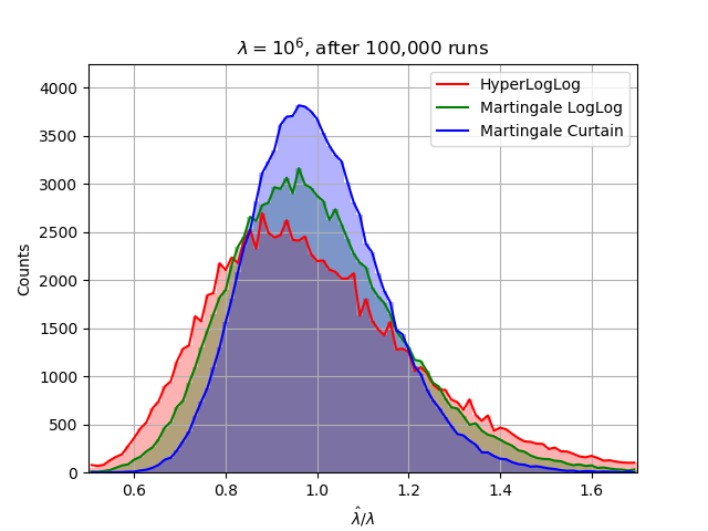
Figure 3: The sketch size is fixed at $128$ bits.

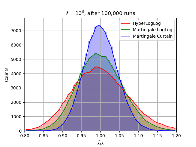
Figure 4: The sketch size is fixed at 1200 bits.

Sketch	Using $128$ bits				Using $1200$ bits
	Experiment		Prediction		Experiment		Prediction
	Var	StdErr	Var	StdErr	Var	StdErr	Var	StdErr
HyperLogLog	$0.0573$	$23.94\%$	$0.0549$	$23.44\%$	$0.00541$	$7.36\%$	$0.00539$	$7.35\%$
Martingale LogLog	$0.0348$	$18.65\%$	$0.0365$	$19.10\%$	$0.00350$	$5.91\%$	$0.00347$	$5.89\%$
Martingale Curtain	$0.0211$	$14.54\%$	$0.0208$	$14.43\%$	$0.00189$	$4.35\%$	$0.00193$	$4.39\%$

Table 2: The relative variance is $\frac{1}{\lambda^{2}}\operatorname{Var}(\hat{\lambda}\mid\lambda)$ and standard error is $\frac{1}{\lambda}\sqrt{\operatorname{Var}(\hat{\lambda}\mid\lambda)}$. The predictions for Martingale LogLog and Martingale Curtain use Theorems 3, 5, and 6. The predictions for HyperLogLog are from Flajolet et al. [19, p. 139].

7 Conclusion

The Martingale transform is attractive due to its simplicity and low variance, but it results in non-mergeable sketches. We proved that under natural assumptions, it generates optimal estimators automatically, allowing one to design structurally more complicated sketches, without having to worry about designing or analyzing ad hoc estimators. We proposed the Curtain sketch, in which each subsketch only needs a constant number of bits of memory, for arbitrarily large cardinality $U$.

The analytic framework of Theorems 2 and 3 simplifies Cohen [14] and Ting [34], and gives a user-friendly formula for the asymptotic relative variance (ARV) of the Martingale estimator, as a function of the sketch’s constant $\kappa$. We applied this framework to Martingale Curtain as well as the Martingale version of the classic sketches ($\mathsf{MinCount}$, $\mathsf{HLL}$ and $\mathsf{PCSA}$).

Assuming perfect compression, one gets the memory-variance product (MVP) of an sketch by multiplying its entropy and ARV. It is proved that for linearizable sketches, Fishmonger is optimal for mergeable sketches [31] (limiting $\textsf{MVP}=H_{0}/I_{2}\approx 1.98$). In this paper we proved that in the sequential (non-mergeable) setting, if we restrict our attention to linearizable sketches, that Martingale Fishmonger is optimal, with limiting $\textsf{MVP}=H_{0}/2\approx 1.63$ (Section 5.2). We conjecture that these two lower bounds hold for general, possibly non-linearizable sketches.

References

- [1] N. Alon, P. B. Gibbons, Y. Matias, and M. Szegedy. Tracking join and self-join sizes in limited storage. In Proceedings 18th ACM Symposium on Principles of Database Systems (PODS), pages 10–20, 1999.
- [2] D. N. Baker and B. Langmead. Dashing: Fast and accurate genomic distances with hyperloglog. bioRxiv, 2019.
- [3] Z. Bar-Yossef, T. S. Jayram, R. Kumar, D. Sivakumar, and L. Trevisan. Counting distinct elements in a data stream. In Proceedings 6th International Workshop on Randomization and Approximation Techniques (RANDOM), volume 2483 of Lecture Notes in Computer Science, pages 1–10, 2002.
- [4] Z. Bar-Yossef, R. Kumar, and D. Sivakumar. Reductions in streaming algorithms, with an application to counting triangles in graphs. In Proceedings 13th Annual ACM-SIAM Symposium on Discrete Algorithms (SODA), pages 623–632, 2002.
- [5] R. Ben-Basat, G. Einziger, S. L. Feibish, J. Moraney, and D. Raz. Network-wide routing-oblivious heavy hitters. In Proceedings of the 2018 Symposium on Architectures for Networking and Communications Systems (ANCS), pages 66–73, 2018.
- [6] J. Błasiok. Optimal streaming and tracking distinct elements with high probability. ACM Trans. Algorithms, 16(1):3:1–3:28, 2020.
- [7] A. Z. Broder. On the resemblance and containment of documents. In Proceedings of Compression and Complexity of SEQUENCES, pages 21–29, 1997.
- [8] T. Buddhika, M. Malensek, S. L. Pallickara, and S. Pallickara. Synopsis: A distributed sketch over voluminous spatiotemporal observational streams. IEEE Trans. Knowl. Data Eng., 29(11):2552–2566, 2017.
- [9] P. Chassaing and L. Gerin. Efficient estimation of the cardinality of large data sets. In Proceedings of the 4th Colloquium on Mathematics and Computer Science Algorithms, Trees, Combinatorics and Probabilities, 2006.
- [10] A. Chen, J. Cao, L. Shepp, and T. Nguyen. Distinct counting with a self-learning bitmap. Journal of the American Statistical Association, 106(495):879–890, 2011.
- [11] M. Chen, S. Chen, and Z. Cai. Counter tree: A scalable counter architecture for per-flow traffic measurement. IEEE/ACM Trans. Netw., 25(2):1249–1262, 2017.
- [12] P. H. Chia, D. Desfontaines, I. M. Perera, D. Simmons-Marengo, C. Li, W. Day, Q. Wang, and M. Guevara. KHyperLogLog: Estimating reidentifiability and joinability of large data at scale. In Proceedings of the 2019 IEEE Symposium on Security and Privacy, pages 350–364, 2019.
- [13] E. Cohen. Size-estimation framework with applications to transitive closure and reachability. J. Comput. Syst. Sci., 55(3):441–453, 1997.
- [14] E. Cohen. All-distances sketches, revisited: HIP estimators for massive graphs analysis. IEEE Trans. Knowl. Data Eng., 27(9):2320–2334, 2015.
- [15] E. Cohen and H. Kaplan. Tighter estimation using bottom sketches. Proc. VLDB Endow., 1(1):213–224, 2008.
- [16] M. Durand and P. Flajolet. Loglog counting of large cardinalities. In Proceedings 11th Annual European Symposium on Algorithms (ESA), volume 2832 of Lecture Notes in Computer Science, pages 605–617. Springer, 2003.
- [17] R. A. L. Elworth, Q. Wang, P. K. Kota, C. J. Barberan, B. Coleman, A. Balaji, G. Gupta, R. G. Baraniuk, A. Shrivastava, and T. J. Treangen. To petabytes and beyond: recent advances in probabilistic and signal processing algorithms and their application to metagenomics. Nucleic Acids Research, 48(10):5217–5234, 2020.
- [18] C. Estan, G. Varghese, and M. E. Fisk. Bitmap algorithms for counting active flows on high-speed links. IEEE/ACM Trans. Netw., 14(5):925–937, 2006.
- [19] P. Flajolet, É. Fusy, O. Gandouet, and F. Meunier. HyperLogLog: the analysis of a near-optimal cardinality estimation algorithm. In Proceedings of the 18th International Meeting on Probabilistic, Combinatorial, and Asymptotic Methods for the Analysis of Algorithms (AofA), 2007.
- [20] P. Flajolet and G. N. Martin. Probabilistic counting algorithms for data base applications. J. Comput. Syst. Sci., 31(2):182–209, 1985.
- [21] M. J. Freitag and T. Neumann. Every row counts: Combining sketches and sampling for accurate group-by result estimates. In Proceedings of the 9th Biennial Conference on Innovative Data Systems Research (CIDR), 2019.
- [22] P. B. Gibbons and S. Tirthapura. Estimating simple functions on the union of data streams. In Proceedings 13th Annual ACM Symposium on Parallel Algorithms and Architectures (SPAA), pages 281–291, 2001.
- [23] F. Giroire. Order statistics and estimating cardinalities of massive data sets. Discret. Appl. Math., 157(2):406–427, 2009.
- [24] A. Helmi, J. Lumbroso, C. Martínez, and A. Viola. Data Streams as Random Permutations: the Distinct Element Problem. In Proceedings of the 23rd International Meeting on Probabilistic, Combinatorial, and Asymptotic Methods for the Analysis of Algorithms (AofA), pages 323–338, 2012.
- [25] P. Indyk and D. P. Woodruff. Tight lower bounds for the distinct elements problem. In Proceedings 44th IEEE Symposium on Foundations of Computer Science (FOCS), October 2003, Cambridge, MA, USA, Proceedings, pages 283–288, 2003.
- [26] T. S. Jayram and D. P. Woodruff. Optimal bounds for Johnson-Lindenstrauss transforms and streaming problems with subconstant error. ACM Trans. Algorithms, 9(3):26:1–26:17, 2013.
- [27] D. M. Kane, J. Nelson, and D. P. Woodruff. An optimal algorithm for the distinct elements problem. In Proceedings 29th ACM Symposium on Principles of Database Systems (PODS), pages 41–52, 2010.
- [28] K. J. Lang. Back to the future: an even more nearly optimal cardinality estimation algorithm. CoRR, abs/1708.06839, 2017.
- [29] J. Lumbroso. An optimal cardinality estimation algorithm based on order statistics and its full analysis. In Proceedings of the 21st International Meeting on Probabilistic, Combinatorial, and Asymptotic Methods in the Analysis of Algorithms (AofA), pages 489–504, 2010.
- [30] G. Marçais, B. Solomon, R. Patro, and C. Kingsford. Sketching and sublinear data structures in genomics. Annual Review of Biomedical Data Science, 2(1):93–118, 2019.
- [31] S. Pettie and D. Wang. Information theoretic limits of cardinality estimation: Fisher meets Shannon. In Proceedings 53rd ACM Symposium on Theory of Computing (STOC), 2021.
- [32] N. Pham. Hybrid LSH: faster near neighbors reporting in high-dimensional space. In Proceedings of the 20th International Conference on Extending Database Technology (EDBT), pages 454–457, 2017.
- [33] B. Scheuermann and M. Mauve. Near-optimal compression of probabilistic counting sketches for networking applications. In Proceedings of the 4th International Workshop on Foundations of Mobile Computing (DIALM-POMC), 2007.
- [34] D. Ting. Streamed approximate counting of distinct elements: beating optimal batch methods. In Proceedings 20th ACM Conference on Knowledge Discovery and Data Mining (KDD), pages 442–451, 2014.
- [35] J. Wires, S. Ingram, Z. Drudi, N. J. A. Harvey, and A. Warfield. Characterizing storage workloads with counter stacks. In Proceedings of the 11th USENIX Symposium on Operating Systems Design and Implementation (OSDI), pages 335–349, 2014.
- [36] D. E. Wood, J. Lu, and B. Langmead. Improved metagenomic analysis with Kraken 2. bioRxiv, 2019.
- [37] Q. Xiao, S. Chen, Y. Zhou, M. Chen, J. Luo, T. Li, and Y. Ling. Cardinality estimation for elephant flows: A compact solution based on virtual register sharing. IEEE/ACM Trans. Netw., 25(6):3738–3752, 2017.