Hidden Devil’s staircase in a two-dimensional elastic model of spin crossover materials

Abstract

Spin crossover (SCO) materials are reversible molecular switches found in a wide range of transition metal complexes and metal organic frameworks (MOFs). They exhibit diverse spin state orderings and transitions between them. We present an exact mapping from an elastic lattice mismatch model to a long-range Ising model, with an inverse square decay of the interaction strengths at large distances (on the square lattice). This provides a microscopic justification for an Ising model description, which has previously only been justified on phenomenological grounds. Elastic frustration is required for non-zero Ising interactions, but whether or not the short-range interactions in the Ising model are geometrically frustrated depends on the ratio of the bulk and shear moduli or equivalently Poisson’s ratio. We show that, for a simple square lattice model with realistic parameters, sweeping the enthalpy difference between the two spin-states at zero temperature leads to a large (probably infinite) number of spin-state orderings and corresponding steps in the fraction of high-spin ions, consistent with a Devil’s staircase. The staircase can also be climbed by varying the temperature, but then some of the steps are hidden and only a finite number remain, consistent with experiments on relevant framework materials, such as {(Fe[Hg(SCN)₃]₂(4,4’-bipy)₂)}_n. Our results are also relevant to other binary systems with lattice mismatch, e.g., heterogeneous solids.

I Introduction

In a Devil’s staircase a physical observable moves through an infinite number of discrete steps as some parameter is varied [1, 2]. Devil’s staircases are continuous everywhere and have zero derivative almost everywhere; nevertheless the observable is not constant. Indeed, as it goes from its minimum value to its maximum value the observable takes every value in between [3, 4]. They can arise in simple systems where there are two competing incommensurate periodicities. Devil’s staircases are found in several dynamical systems [1], the anisotropic next-nearest-neighbor Ising (ANNNI) model in three dimensions[5, 6, 7], and the one-dimensional Ising model with long-range anti-ferromagnetic interactions [8]. Recently, based on experimental results it has been suggested that a Devil’s staircase may exist in some spin crossover materials [9].

Spin crossover molecules can exist in one of two different electronic states, one low spin (LS) and one high spin (HS), with pronounced differences in geometry, magnetism, and colour. A transition between these states can be induced by a range of physical perturbations, such as temperature  [10], light irradiation [11], pressure [12], magnetic fields [13], and electric fields [14]. The SCO phenomenon has been well documented in octahedral transition metal complexes with $d^{4}-d^{7}$ electron configurations [15]. The molecular bistability of these systems has attracted great interest from the nanoscience community, as this phenomenon has potential applications in data storage and display devices [16, 15]. This interest can be evidenced by the fact that since the discovery of thermally induced SCO, several hundreds of SCO complexes have been synthesised and studied [17]. Furthermore, the change in electronic configuration is accompanied by drastic structural (volume, shape) [18], colour [16] and magnetic changes; these characteristics could have potential applications in mechanical nanoscale machines [19], smart pigments, and optical switches [18].

SCO systems have been reported to present collective phenomena including hysteresis, multistep transitions, gradual transitions, and a variety of spin-state orderings, such as anti-ferroelastic phases [15, 17]. Cooperative interactions between molecules are a key factor in understanding spin-state phase transitions; as a consequence, experimental advances have been accompanied by theoretical investigations aimed at determining the physical origin of this cooperativity. A wide variety of models have been proposed to explain the microscopic origin of spin-state transitions; Ising-like models, specially the Wajnflasz and Pick (WP) model [20], macroscopic thermodynamical models (such as that due to Slichter and Drickamer[21]), and Landau type models, have been extensively used because of their simplicity and generality [15]. However, the origin of their interaction parameters is unclear given the dramatic simplifications they employ. Refs. 15, 17 review a range models that have been used. All of these models reproduce some characteristics, like gradual and abrupt spin-state transitions, multi-step transitions, incomplete transitions, and hysteretic behaviour [15, 17, 22].

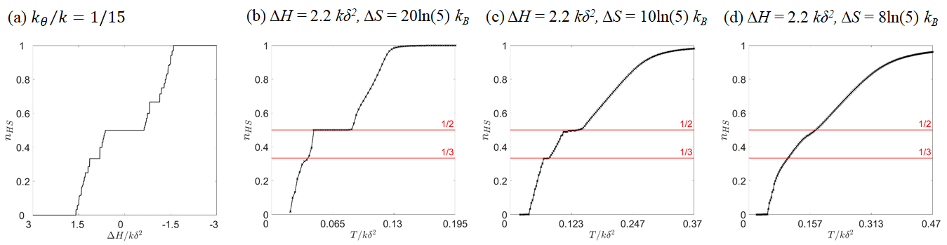
Figure 1: The Devil’s staircase in the fraction of HS metal ions, $n_{HS}$, on sweeping $\Delta H$ at zero temperature (a) is partially hidden when the temperature is varied at fixed $\Delta H$ (b-d). This can be straightforwardly understood as in both cases the transitions are driven by varying $\Delta G=\Delta H-T\Delta S$, so the zero temperature plot (a) is equivalent to the $\Delta S\rightarrow\infty$ limit (note that the $x$-axis is reversed in (a)). As $\Delta S$ increases (moving right to left in the figure) the Devil’s staircase is gradually revealed, i.e., the transitions become sharper and plateaus flatter, and the transition curves increasingly resemble the $T=0$ $n_{HS}$ curve. The horizontal red lines indicate the fraction of HS metals for the phases with the largest areas in the $T=0$ phase diagram when $\Delta H>0$, see Fig. 7, and with the orderings shown in Fig. 8. In all panels $k_{\theta}/k=1/15$. Similar results for different $\Delta H$ and $k_{\theta}/k$ are shown in Figs. 9 and S5. Finite temperature plots are from parallel tempering simulations.

Even though the previously mentioned models have been able to capture many observed phenomena, recent advances in experimental methods, particularly in determining the spatial ordering of spin states, underline the necessity of more realistic theoretical approaches [17]. It is believed that the cooperativity between molecules has an elastic origin; this interaction arises from the pronounced volume change (ca. 25% in FeN₆ environments [18]) of the SCO molecules upon spin change [17]. This difference in volume leads to elastic strains and local deformations of the system’s lattice, which may in turn lead to complicated long and short range interactions. Accordingly, it is desirable to have a model with elastic interactions that leads to the emergence of both short and long range interactions.

Models that explicitly take into account structural degrees of freedom have been proposed, the majority of them are ball and spring models with a lattice mismatch. They have been solved via a variety methods including purely Monte Carlo methods [23, 24], purely molecular dynamics methods [25, 26], and a combination of Monte Carlo methods with damped dynamics [27, 28]. These models have been able to show first order and gradual one- and two-step phase transitions. It was observed some time ago that the structure of the SCO crystals qualitatively influences the observed spin-crossover phenomena [29, 30]; however, only recently have detailed structure-property relationships begun to be identified [31].

Here we present a method, based on a displaced oscillator transformation, to exactly map an elastic system of balls and springs to an Ising model with long-range interactions. We apply this mapping to the square lattice, but the method can readily be applied to other geometries and other elastic models. We show that the Ising coupling constants arise purely from the elastic interactions and give explicit relationships between the bulk and shear moduli and the Ising parameters. For reasonable parameters, the Ising model is geometrically frustrated and multistep transitions naturally occur in this model. We also note the relevance of our model to the physically similar problem of elastic interactions in binary alloys [32, 33].

At zero temperature we find that the system passes through a large (probably infinite) number of spin-state orderings and the associated steps in the fraction of HS metal ions, as the enthalpy difference between the two spin-states ($\Delta H$) decreases (Fig. 1a). This and the variation of the step widths are consistent with a Devil’s staircase. The widths of many of the steps are extremely narrow, as a consequence we only observe a few of them in the finite temperature simulations, where the shape of the $n_{HS}$ curves is similar to the zero temperature case (Figs. 1b, c, and d). Trzop et al. [9] reported a staircase-like thermal conversion of the HS molecular fraction for the bimetallic 2D coordination polymer {(Fe[Hg(SCN)₃]₂(4,4’-bipy)₂)}_n; here they found two wide plateaus at $n_{HS}=0.5$ and $0.34$. The ordering of HS/LS metal centres at $n_{HS}=0.5$ is Néel along the 2D planes (cf. Fig. 8a). At $n_{HS}=0.34$ they report an incommensurate ordering. The thermal conversion curve closely resembles the $n_{HS}$ curves we obtain in our finite temperature simulations (Fig. 1c), where the two most resilient plateaus are at $n_{HS}=1/2$ with Néel ordering and $n_{HS}=1/3$ with diagonal stripe ordering (Figs. 8a and c).

II Mapping an elastic model to an Ising model

We consider a square lattice in two spatial dimensions, with the arrangement of metals and ligands depicted in Fig. 2; with only nearest-neighbour elastic interactions, and a harmonic potential on the angle $\theta$ between adjacent metal-ligand bonds, Fig. 2. Even though the following discussion focuses on a square lattice, the method used can be readily extended to other elastic models and lattices.

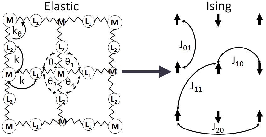
Figure 2: Mapping from a balls and springs model to an Ising model. (Left) Schematic illustration of a square lattice of metal ions (M) connected to ligands (L₁, L₂) by springs; smaller circles represent metals in the LS state, and larger circles in the HS state; $k$ is the elastic constant of the springs, and $k_{\theta}$ corresponds to the elastic constant for bending. Each $M$ has four corresponding angle variables $\theta$, see Eq. (1). (Right) Schematic illustration of the corresponding Ising model on a square lattice; the $J_{nm}$’s are the Ising coupling constants. Up arrows represent a metal in the HS state, and down arrows in the LS state.

This model is appropriate for modeling the in-plane physics of the 1$n$02 family of frameworks [34, 31], with the chemical formula $[M(L^{\prime})_{n}(L)_{2}]$, where $M$ is the SCO active metal, $L$ is the in-plane ligand, $L^{\prime}$ is the interlayer ligand, and $n=1$ or 2 for bridging and monodentate ligands respectively. The $L^{\prime}$ ligand is not explicitly described by this model. A typical member of this family is [Fe(azpy)₂(NCS)₂], where azpy is trans-4,4’-azopyridine [35]. The model can also serve to describe the 1$n$24 family of Hoffmann frameworks [36, 31]. These have the generic formula $[M(L^{\prime})_{n}\{M^{\prime}(L)_{2}\}_{2}]$, where $M^{\prime}$ is a non-SCO-active metal. A typical example is [Fe(pz){Au(CN)₂}₂], where pz is pyrazine [36]. In this case the ‘ligands’ in the model actually describe the composite $M^{\prime}(L)_{2}$ groups.

The Hamiltonian describing this system is

$$H = H_{\sigma}+K+V,$$ (1)

where the three terms are respectively, the free energy difference for each spin state, the kinetic energy of the metal ions and ligands, and the elastic energy of the system.

$$H_{\sigma} = \frac{1}{2}\sum_{i\in\mathbb{Z}_{N_{x}}}\sum_{j\in\mathbb{Z}_{N_{y}}}\left(\Delta H-T\Delta S\right)\sigma_{i,j},$$ (2)

$$K = \sum_{i\in\mathbb{Z}_{N_{x}}}\sum_{j\in\mathbb{Z}_{N_{y}}}\frac{\bm{p}_{M,i,j}^{2}}{2m_{M}}+\frac{\bm{p}_{{L_{1}},i+\frac{1}{2},j}^{2}}{2m_{L_{1}}}+\frac{\bm{p}_{L_{2},i,j+\frac{1}{2}}^{2}}{2m_{L_{2}}},$$ (3)

$$V = \sum_{i\in\mathbb{Z}_{N_{x}}}\sum_{j\in\mathbb{Z}_{N_{y}}}\bigg{[}\frac{k}{2}\left(|\bm{r}_{{L_{1}},i+\frac{1}{2},j}-\bm{r}_{M,i,j}|-\overline{R}-\delta\sigma_{i,j}\right)^{2}$$ (4)

$$\hskip 28.45274pt+\frac{k}{2}\left(|\bm{r}_{M,i,j}-\bm{r}_{{L_{1}},i-\frac{1}{2},j}|-\overline{R}-\delta\sigma_{i,j}\right)^{2}$$

$$\hskip 28.45274pt+\frac{k}{2}\left(|\bm{r}_{{L_{2}},i,j+\frac{1}{2}}-\bm{r}_{M,i,j}|-\overline{R}-\delta\sigma_{i,j}\right)^{2}$$

$$\hskip 28.45274pt+\frac{k}{2}\left(|\bm{r}_{M,i,j}-\bm{r}_{{L_{2}},i,j-\frac{1}{2}}|-\overline{R}-\delta\sigma_{i,j}\right)^{2}$$

$$\hskip 28.45274pt+\frac{k_{\theta}}{2}\overline{R}^{2}\sum_{n=1}^{4}\sin^{2}\left(\frac{\pi}{2}-\theta_{i,j,n}\right)\bigg{]}.$$

We have assigned a pseudo-spin variable $\sigma$ to each metal atom, such that $\sigma=1$ if the metal is in the high spin (HS) state, and $\sigma=-1$ if it is in the low spin (LS) state. The volume of a SCO molecule decreases when going from the HS state to the LS state, as such the minimum energy metal-ligand separation is dependent on the spin-state of the metal: we set $\overline{R}=(R_{HS}+R_{LS})/2$, $\delta=(R_{HS}-R_{LS})/2$, where $R_{HS}$ ($R_{LS}$) is the equilibrium distance between the centre of a metal atom in the HS (LS) state and the center of a nearest neighbour ligand. $\Delta H$ and $\Delta S$ are the enthalpy and entropy difference between the HS and LS states of a single metal center, $T$ is temperature, $\bm{r}_{\nu,i,j}$ and $\bm{p}_{\nu,i,j}$ are the position and momentum of a group, where $\nu=M$, ${L_{1}}$, or ${L_{2}}$ labels the species of the group. Note that $i$ and $j$ are both integers for the metals, but one of them is a half-odd-integer for every ligand. $m_{\nu}$ is the mass of species $\nu$, $k$ is the elastic constant of the springs, and $N=N_{x}\times N_{y}$, is the number of unit cells.

We define

$$\bm{R}_{i,j} = 2i\overline{R}\hat{x}+2j\overline{R}\hat{y},$$ (5)

$$\bm{r}_{\nu,i,j} = \bm{R}_{i,j}+\bm{u}_{\nu,i,j}.$$ (6)

It is important to note that $\bm{u}_{\nu,i,j}=(u^{(x)}_{\nu,i,j},u^{(y)}_{\nu,i,j})$ are displacements about $\bm{R}_{i,j}$ rather than the equilibrium positions of the particles. We can think of the lattice formed by $\bm{R}_{i,j}$ as an “average” lattice; this construction will simplify our calculations below.

The harmonic approximation, $|\bm{u}_{M,i,j}-\bm{u}_{{L_{1}},i-\frac{1}{2},j}|\ll\overline{R}$, is implicit in any elastic model. Therefore, without loss of generality

$$|\bm{r}_{M,i,j}-\bm{r}_{{L_{1}},i-\frac{1}{2},j}| = |\bm{u}_{M,i,j}-\bm{u}_{{L_{1}},i-\frac{1}{2},j}+\overline{R}\hat{\bm{x}}|$$ (7)

$$= u^{(x)}_{M,i,j}-u^{(x)}_{{L_{1}},i-\frac{1}{2},j}+\overline{R}.$$

Similar results follow for $|\bm{u}_{M,i,j}-\bm{u}_{{L_{2}},i,j-\frac{1}{2}}|$, $|\bm{u}_{{L_{1}},i+\frac{1}{2},j}-\bm{u}_{M,i,j}|$, and $|\bm{u}_{{L_{2}},i,j+\frac{1}{2}}-\bm{u}_{M,i,j}|$. Hence, $V=V_{u}+V_{u\sigma}$, where

$$V_{u} = \sum_{i\in\mathbb{Z}_{N_{x}}}\sum_{j\in\mathbb{Z}_{N_{y}}}\left[\frac{k}{2}\left(u^{(x)}_{{L_{1}},i+\frac{1}{2},j}-u^{(x)}_{M,i,j}\right)^{2}\right.$$ (8)

$$\left.+\frac{k}{2}\left(u^{(x)}_{M,i,j}-u^{(x)}_{{L_{1}},i-\frac{1}{2},j}\right)^{2}+\frac{k}{2}\left(u^{(y)}_{{L_{2}},i,j+\frac{1}{2}}-u^{(y)}_{M,i,j}\right)^{2}\right.$$

$$\left.+\frac{k}{2}\left(u^{(y)}_{M,i,j}-u^{(y)}_{{L_{2}},i,j-\frac{1}{2}}\right)^{2}\right.$$

$$\left.+\frac{k_{\theta}}{2}\left(u^{(x)}_{{L_{2}},i,j+\frac{1}{2}}-u^{(x)}_{M,i,j}+u^{(y)}_{{L_{1}},i+\frac{1}{2},j}-u^{(y)}_{M,i,j}\right)^{2}\right.$$

$$\left.+\frac{k_{\theta}}{2}\left(u^{(x)}_{M,i,j}-u^{(x)}_{{L_{2}},i,j+\frac{1}{2}}+u^{(y)}_{{L_{1}},i-\frac{1}{2},j}-u^{(y)}_{M,i,j}\right)^{2}\right.$$

$$\left.+\frac{k_{\theta}}{2}\left(u^{(x)}_{{L_{2}},i,j-\frac{1}{2}}-u^{(x)}_{M,i,j}+u^{(y)}_{{L_{1}},i-\frac{1}{2},j}-u^{(y)}_{M,i,j}\right)^{2}\right.$$

$$\left.+\frac{k_{\theta}}{2}\left(u^{(x)}_{{L_{2}},i,j-\frac{1}{2}}-u^{(x)}_{M,i,j}+u^{(y)}_{M,i,j}-u^{(y)}_{{L_{1}},i+\frac{1}{2},j}\right)^{2}\right],$$

and

$$V_{u\sigma} = \sum_{i\in\mathbb{Z}_{N_{x}}}\sum_{j\in\mathbb{Z}_{N_{y}}}\left[u^{(x)}_{{L_{1}},i-\frac{1}{2},j}-u^{(x)}_{{L_{1}},i+\frac{1}{2},j}\right.$$ (9)

$$\hskip 14.22636pt\left.+u^{(y)}_{{L_{2}},i,j-\frac{1}{2}}-u^{(y)}_{{L_{2}},i,j+\frac{1}{2}}\right]k\delta\sigma_{i,j}.$$

Next, we Fourier transform the generalized coordinates of our system, with $\alpha\in\{x,y\}$

$$u^{(\alpha)}_{M,i,j} = \frac{1}{\sqrt{N_{x}N_{y}}}\sum_{\bm{q}}e^{i\bm{q}\cdot\bm{R}_{i,j}}u^{(\alpha)}_{M,\bm{q}},$$ (10)

$$u^{(\alpha)}_{{L_{1}},i+\frac{1}{2},j} = \frac{1}{\sqrt{N_{x}N_{y}}}\sum_{\bm{q}}e^{i\bm{q}\cdot\bm{R}_{i+\frac{1}{2},j}}u^{(\alpha)}_{L_{1},\bm{q}},$$ (11)

$$u^{(\alpha)}_{{L_{2}},i,j+\frac{1}{2}} = \frac{1}{\sqrt{N_{x}N_{y}}}\sum_{\bm{q}}e^{i\bm{q}\cdot\bm{R}_{i,j+\frac{1}{2}}}u^{(\alpha)}_{L_{2},\bm{q}}.$$ (12)

This yields

$$K = \sum_{\bm{q}}\bigg{[}\frac{\bm{p}_{M,\bm{q}}\cdot\bm{p}_{M,-\bm{q}}}{2m_{M}}+\frac{\bm{p}_{L_{1},\bm{q}}\cdot\bm{p}_{L_{1},-\bm{q}}}{2m_{L_{1}}}$$ (13)

$$+\frac{\bm{p}_{L_{2},\bm{q}}\cdot\bm{p}_{L_{2},-\bm{q}}}{2m_{L_{2}}}\bigg{]}$$

and

$$V_{u} = \sum_{\bm{q}}\bigg{[}ku^{(x)}_{L_{1},\bm{q}}u^{(x)}_{L_{1},-\bm{q}}-2k\cos(q_{x}\overline{R})u^{(x)}_{M,\bm{q}}u^{(x)}_{L_{1},-\bm{q}}$$ (14)

$$\hskip 2.84544pt+(k+2k_{\theta})u^{(x)}_{M,\bm{q}}u^{(x)}_{M,-\bm{q}}+ku^{(y)}_{L_{2},\bm{q}}u^{(y)}_{L_{2},-\bm{q}}$$

$$-2k\cos(q_{y}\overline{R})u^{(y)}_{M,\bm{q}}u^{(y)}_{L_{2},-\bm{q}}+2k_{\theta}u^{(x)}_{L_{2},\bm{q}}u^{(x)}_{L_{2},-\bm{q}}$$

$$+(k+2k_{\theta})u^{(y)}_{M,\bm{q}}u^{(y)}_{M,-\bm{q}}+2k_{\theta}u^{(y)}_{L_{1},\bm{q}}u^{(y)}_{L_{1},-\bm{q}}$$

$$-4k_{\theta}\big{(}\cos(q_{y}\overline{R})u^{(x)}_{M,\bm{q}}u^{(x)}_{L_{2},-\bm{q}}+\cos(q_{x}\overline{R})u^{(y)}_{M,\bm{q}}u^{(y)}_{L_{1},-\bm{q}}$$

$$-\sin(q_{x}\overline{R})\sin(q_{y}\overline{R})u^{(x)}_{L_{2},\bm{q}}u^{(y)}_{L_{1},-\bm{q}}\big{)}\bigg{]}$$

We rewrite $V_{u}$ as

$$V_{u}=\frac{1}{2}\sum_{\bm{q},\alpha,\alpha^{\prime},\nu,\nu^{\prime}}\left(\mathrm{f}^{\alpha,\alpha^{\prime}}_{\nu,\nu^{\prime},\bm{q}}u^{(\alpha)}_{\nu,\bm{q}}u^{(\alpha^{\prime})}_{\nu^{\prime},\bm{-q}}\right)\equiv\frac{1}{2}\sum_{\bm{q}}\bm{u}_{\bm{q}}^{T}\mathrm{F}_{\bm{q}}\bm{u}_{\bm{-q}},$$ (15)

$\mathrm{F}_{\bm{q}}$ is the Hessian matrix whose elements are

$$\mathrm{f}^{\alpha,\alpha^{\prime}}_{\nu,\nu^{\prime},\bm{q}}=\frac{\partial^{2}V_{u}}{\partial u^{(\alpha)}_{\nu,\bm{q}}\partial u^{(\alpha^{\prime})}_{\nu^{\prime},\bm{-q}}}.$$ (16)

We diagonalize $V_{u}$ by writing the eigenvalue problem

$$\kappa_{\bm{q}}\bm{\psi}_{\bm{q}}=\mathrm{F}_{\bm{q}}\bm{\psi}_{\bm{q}},$$ (17)

and find the eigenvalues, $\kappa_{\bm{q}}$, and normalized eigenvectors, $\bm{\psi}_{\bm{q}}$, such that

$$\bm{u}_{\bm{q}}^{T}\mathrm{F}_{\bm{q}}\bm{u}_{\bm{-q}}=\bm{Q}^{T}_{\bm{q}}D_{\bm{q}}\bm{Q}_{\bm{-q}},$$ (18)

where $\bm{Q}_{\bm{q}}=U^{T}_{\bm{q}}\bm{u}_{\bm{q}}$, $\bm{u}_{\bm{q}}$ is a six-dimensional column vector whose components are $u^{(\alpha)}_{\nu,\bm{q}}$, $U_{\bm{q}}$ is a square matrix whose columns are $\bm{\psi}_{\bm{q}}$, and $D_{\bm{q}}$ is a diagonal matrix whose elements are $\kappa_{\bm{q}}$. With this transformation $u^{(\alpha)}_{\nu,i,j}$ takes the form

$$u^{(\alpha)}_{\nu,i,j}=\frac{1}{\sqrt{N_{x}N_{y}}}\sum_{\mu,\bm{q}}e^{i\bm{q}\cdot\bm{R}_{i,j}}Q_{\mu,\bm{q}}\psi^{(\alpha)\mu}_{\nu,\bm{q}},$$ (19)

where $\mu=1,\dots,6$ enumerates the eigenvalues of the Hessian matrix, $Q_{\mu,\bm{q}}$ are the components of the column vector $\bm{Q}_{\bm{q}}$, and $\psi^{(\alpha)\mu}_{\nu,\bm{q}}$ are the components of the orthonormal eigenvectors $\bm{\psi}^{\mu}_{\bm{q}}$. With this change of basis

$$V_{u}=\frac{1}{2}\sum_{\mu,\bm{q}}\kappa_{\mu,\bm{q}}Q_{\mu,\bm{q}}Q_{\mu,\bm{-q}}$$ (20)

and

$$V_{u\sigma}=\sum_{\mu,\bm{q}}\xi_{\mu}(\bm{q})Q_{\mu,\bm{q}}\sigma_{-\bm{q}},$$ (21)

where

$$\xi_{\mu}(\bm{q})=-2i\delta k\left[\psi^{(x)\mu}_{L_{1},\bm{q}}\sin(q_{x}\overline{R})+\psi^{(y)\mu}_{L_{2},\bm{q}}\sin(q_{y}\overline{R})\right],$$ (22)

and

$$\sigma_{i,j}=\frac{1}{\sqrt{N_{x}N_{y}}}\sum_{\bm{q}}e^{i\bm{q}\cdot\bm{R}_{i,j}}\sigma_{\bm{q}}.$$ (23)

Now we make a displaced oscillator transformation, which defines

$$v_{\mu,\bm{q}} = Q_{\mu,\bm{q}}+\frac{\xi_{\mu}(-\bm{q})}{\kappa_{\mu,\bm{q}}}\sigma_{\bm{q}}.$$ (24)

This is essentially “completing the square” so that the interaction between $Q$ and $\sigma$ is replaced by an interaction between pseudo-spins. This is mathematically analogous to treatments of the co-operative Jahn-Teller effect [37, 38]. The Hamiltonian then takes the form

$$H = H_{v}+H_{\sigma}+H_{\sigma\sigma},$$ (25)

where

$$H_{v} = K+\frac{1}{2}\sum_{\mu,\bm{q}}\kappa_{\mu,\bm{q}}v_{\mu,\bm{q}}v_{\mu,-\bm{q}},$$ (26)

and

$$H_{\sigma\sigma} = -\frac{1}{2}\sum_{\mu,\bm{q}}\frac{|\xi_{\mu}(\bm{q})|^{2}}{\kappa_{\mu,\bm{q}}}\sigma_{\bm{q}}\sigma_{-\bm{q}}$$ (27)

$$= \frac{1}{2}\sum_{i,j,n,m}J_{n,m}\sigma_{i,j}\sigma_{i+n,j+m},$$

where we identify $J_{nm}$ as the Ising coupling constants between sites $i,j$ and $i+n,j+m$,

$$J_{n,m} = -\frac{1}{N_{x}N_{y}}\sum_{\mu,\bm{q}}\frac{|\xi_{\mu}(\bm{q})|^{2}}{\kappa_{\mu,\bm{q}}}e^{i\bm{q}\cdot(\bm{R}_{i,j}-\bm{R}_{i+n,j+m})}$$

$$= \sum_{\mu}J^{\mu}_{n,m},$$

where,

$$J^{\mu}_{n,m}=-\frac{\overline{R}^{2}}{\pi^{2}}\int_{BZ}d^{2}\bm{q}\frac{|\xi_{\mu}(\bm{q})|^{2}}{\kappa_{\mu,\bm{q}}}\cos\left[2q_{x}\overline{R}n+2q_{y}\overline{R}m\right],$$ (29)

and the integral over the first Brillouin zone is defined as $\int_{BZ}=\int_{-(\pi/2\overline{R})}^{(\pi/2\overline{R})}\int_{-(\pi/2\overline{R})}^{(\pi/2\overline{R})}$ and in the final equality we have taken the limit $N_{x},N_{y}\rightarrow\infty$.

The final expression for $H$ is

$$H = \frac{1}{2}\sum_{i,j}\left(\Delta H-T\Delta S\right)\sigma_{i,j}+\frac{1}{2}\sum_{i,j,n,m}J_{n,m}\sigma_{i,j}\sigma_{i+n,j+m}$$ (30)

$$+H_{v}.$$

As $H_{v}$ is independent of the $\sigma_{i,j}$ (Eq. (26)) the elastic degrees of freedom and the pseudospins are decoupled.

$J_{n,m}$ can be evaluated exactly in a few special cases. If we set $k_{\theta}=0$, the eigenvalues and eigenvectors of the Hessian take a simple analytical form, and the Ising coupling constants, between metal sites ($i,j$) and ($i+n,j+m$), are given by

$$J_{n,m}=-4k\delta^{2}\frac{1}{4\pi^{2}}\int\limits_{-\pi}^{\pi}\int\limits_{-\pi}^{\pi}d\phi d\phi^{\prime}\cos\left[\phi n+\phi^{\prime}m\right]=0,$$ (31)

for all $n,m\in\mathbb{Z}$, where $\phi=2\overline{R}q_{x}$, $\phi^{\prime}=2\overline{R}q_{y}$.

Similarly, for a one-dimensional chain in one spatial dimension (and therefore with no bending possible), the contributions from the different eigenvalues/eigenvectors of the Hessian matrix cancel each other out, this leads to no Ising interactions between the metal centres. This is because the chain will simply increase or decrease in length to accommodate the metal centres with different spin states. This result is also consistent with the one-dimensional model presented by Boukheddaden, et. al. [39]; in their model, spin crossover molecules are connected by springs whose elastic constants depend on the spin states of the molecules. In the case where all elastic constants are equal the Ising coupling constants vanish.

Again, the Ising coupling constants of our model vanish for the cubic lattice without angular interactions. This shows that the existence of cooperativity reflects the inability of the lattice to accommodate the change in geometry associated with a spin state change [30, 29]. When $k_{\theta}$ is zero the lattice can accommodates a change in size of a molecule with zero energy cost.

The Ising coupling constants scale with $k\delta^{2}$, which is the energy scale associated with a spin state change of a metal ion; the size of the hysteresis scales with the magnitude of the Ising coupling constants [40], therefore our model predicts that the hysteresis scales with the rigidity of the lattice and with the change in size of the SCO molecules and that a wide hysteresis does not require a crystallographic phase change during spin crossover, consistent with experiments [30].

It is important to note that the origin of the Ising coupling constants is purely from the elastic interactions. They are independent of the mass of the ligands and metals, and do not depend on the dynamics of the system, see Appendix A. However, isotopic substitutions are expected to change $\Delta H$ (due to zero-point energy changes) and $\Delta S$ (which is dominated by the vibrational contribution to the entropy). This is consistent with the experimental observation that isotopic substitution tends to lead to shifts in critical temperatures and changes in the width of hysteresis, but has not been observed to dramatically change the spin-state ordering, see Appendix B for a brief review of these experiments.

III Evaluation of the Ising coupling constants

For $k_{\theta}>0$, the Ising coupling constants are non-zero; however, the eigenvalues/eigenvectors of the Hessian cannot be computed analytically. Therefore we perform the integral numerically, unless otherwise stated we use a $2\,000\times 2\,000$ Monkhorst-Pack [41] grid and set $\overline{R}=49\delta$ (see Sec. IV for further details).

III.1 Short-range behaviour

We report the near neighbour couplings for representative $k_{\theta}/k$ in Fig. 3 and the $k_{\theta}/k$ dependence of selected $J_{n,m}$ in Fig. 4. $J_{1,0}$ is always positive (i.e., antiferromagnetic) and $J_{1,1}$ is always negative (i.e., ferromagnetic). However, the signs of many of the other the $J_{n,m}$ change as $k_{\theta}/k$ varies. For example, for small $k_{\theta}/k$, the $J_{n,0}$ are all positive, but as the ratio approaches unity, they become negative for $n>1$, only $J_{1,0}$ remains positive.

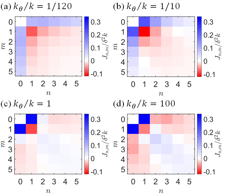
Figure 3: Short-range spatial dependence of the Ising interactions, for different values of $k_{\theta}/k$. There is significant frustration for $k_{\theta}/k\ll 1$, but as $k_{\theta}/k$ increases this is lifted and the near neighbour interactions cooperate to stabilize Néel order.

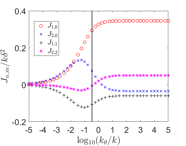
Figure 4: Dependence of selected Ising couplings on the relative stiffnesses to bending, $k_{\theta}$, and stretching, $k$. As $k_{\theta}$ varies, the signs of all the Ising constants other than $J_{1,0}$ and $J_{1,1}$ change. For increasing $k_{\theta}$, $J_{1,0}$ increases, but the other Ising coupling constants vary non-monotonically. However, for $k_{\theta}/k>1$ all the Ising interactions approach constant values. For $k_{\theta}/k<0.013$, $J_{2,0}$ is slightly larger than $J_{1,0}$, and as $k_{\theta}$ approaches $0$, all Ising couplings vanish, consistent with the analytical result for $k_{\theta}=0$, Eq. (31). For $k_{\theta}/k>1$, the Ising coupling constants approach constant values. $J_{1,0}$ is always positive and $J_{1,1}$ is always negative, but the signs of $J_{2,0}$ and $J_{2,2}$ depend on $k_{\theta}/k$. The vertical black line indicates the maximum physically reasonable value for $k_{\theta}/k$ in an isotropic material, see Fig. 6

For large $k_{\theta}/k$ the Ising coupling constants approach constant values. As $k_{\theta}/k$ gets larger, the magnitude of $J_{1,0}$ becomes larger and increases faster than any of the other $J_{n,m}$. Hence, $k_{\theta}/k$ controls the frustration and cooperativity in the system. For example, for $k_{\theta}/k\ll 1$ (Fig. 3a) the magnitudes of the Ising coupling constants are comparable, which will introduce significant frustration. At $k_{\theta}/k=1$ (Fig. 3c) $J_{1,0}$ and $J_{1,1}$ are much larger than the other Ising coupling constants. However, $J_{1,0}>0$ and $J_{1,1}<0$ therefore, they cooperate in stabilizing Néel order, which is commonly observed in the 1$n$02 [31, 42, 35, 43, 44, 45] and 1$n$24 [31, 46, 47, 48, 49, 50, 51, 52, 53] families. However, the other short-range interactions remain important and other long-range ordered phases may also be stabilized, as we will discuss in Section V. For $k_{\theta}/k\gg 1$ (Fig. 3d) $J_{1,0}$ has a much larger magnitude than the other $J_{n,m}$. Therefore, the short-range interactions continue to favor Néel order.

Surprisingly, when $k_{\theta}/k$ is sufficiently small, $J_{2,0}$ can be larger than $J_{1,0}$. However, all $J_{n,m}$ vanish as $k_{\theta}/k$ approaches zero, consistent with the analytical result for $k_{\theta}=0$, Eq. (31). As $k_{\theta}/k\rightarrow 0$, the shear modulus vanishes and the lattice can accommodate spin state changes with no energy cost. In different words, there is no elastic frustration.

Our expression (Eq. (II)) for the Ising couplings consists of a decomposition into different contributions from the six different eigenvectors (elastic modes) of the Hessian matrix (Eq. (16)). One might hope to gain some physical insight from looking at the relative contributions from the different modes and how they vary as the parameter ratio $k_{\theta}/k$ varies. Relevant plots of both the different contributions and the mode dispersion relations are shown in the Supplementary material [54]. It is not possible to make many generalisations about the relative contributions and how they vary with $k_{\theta}/k$. All modes contribute significantly, except when $k_{\theta}/k$ becomes larger than one, the contributions of modes with the three largest eigenvalues become negligible. For all the Ising couplings the relative sign of the contributions from the different modes changes as $k_{\theta}/k$ varies, indicating a subtle competition between the different modes.

III.2 Long range behaviour

For large separations between metal centers, the Ising coupling constants follow a power law decay. On the square lattice we find an inverse square law: Fig. 5 demonstrates that $|J_{n,0}|=An^{-2}$ and $|J_{n,n}|=Bn^{-2}$ for large $n$, where $A$ and $B$ are constants that depend on the ratio $k_{\theta}/k$. This is very different from previous approximate derivations of Ising models for SCO materials, which either only contain short-range interactions [15, 55] or result in infinite range interactions (that are independent of the separation between metal centers) [55, 56, 57, 31, 33, 58, 59].

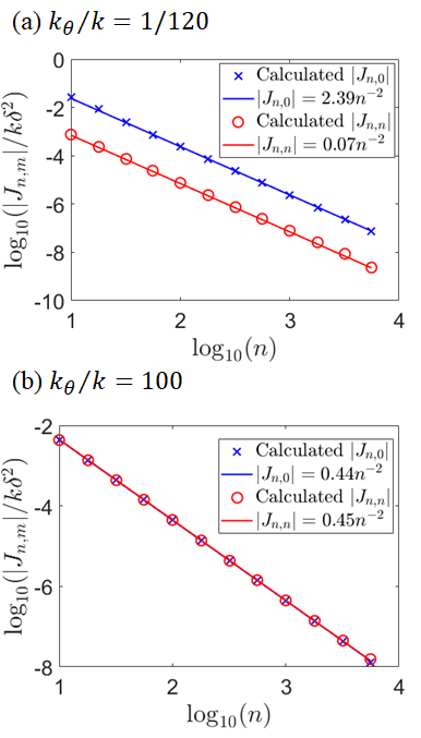
Figure 5: Logarithmic plots of $|J_{n,0}|$ and $|J_{n,n}|$ as a function of $n$, displaying power law behaviour for large $n$, irrespective of the ratio $k_{\theta}/k$. Prefactors were determined from linear fits where performed using a least-squares method. The Ising coupling constants were calculated using a $50\,000\times 50\,000$ grid.

It has recently been proposed that spin-state ices can occur in SCO materials on frustrated lattices [59, 60]. This phase is not characterized by a spontaneously broken symmetry, but rather by a local constraint or ice-rule. On the kagome lattice this dictates that each triangle contains two HS and one LS metals (or vice versa). The low energy excitations are fractionalized particles with a spin intermediate between the HS and LS states. Whether or not these quasiparticles are deconfined (and hence whether the spin-state ice exists) depends on the nature of the long-range interactions.

In particular an infinite-range interaction suppresses spin-state ice. Consequently, previous work [59, 60] only finds spin-state ice in regions of parameter space where the infinite-range interaction is very weak. In contrast, long-range interactions that obey an inverse square law do not suppress ice phases [61]. Therefore, our finding that the long-range interactions obey a power law suggest that spin-state ice phases are more stable than has been previously appreciated.

It has also been shown [55, 56, 57] that the details of the long-range interaction are important for accurately describing the thermodynamics and critical behavior of SCO materials. Therefore, the proper characterization of the long-range interactions is necessary for an accurate modeling of experiments.

IV Parameter values

In order to extract values for the spring constants, we can use the bulk modulus derived for a cubic lattice with nearest neighbours elastic interactions [62]

$$B=\frac{1}{6}k\left(\frac{N}{V_{o}}\right)^{1/3},$$ (32)

where $N$ is the total number of unit cells, $k$ is the spring constant between nearest neighbours, and $V_{o}$ is the volume of the system at equilibrium. Eq. (32) differs by a factor of $1/2$ from the expression in [62], because in our case we have two springs between neighbouring metal sites. With this expression we can use experimental values to estimate $k$. For a cubic lattice $V_{o}/N\approx(2\overline{R})^{3}$, substituting this into Eq. (32)

$${k}={12\overline{R}B}.$$ (33)

Typically bulk moduli in frameworks and SCO complexes are $B=2-50$ GPa [63, 64, 65, 66, 67]. $\overline{R}$ is just the distance between metal sites; typically $2\overline{R}=6-10$ Å. Thus, $k=12-300$ N/m.

For the elastic constant involved in angular interactions, $k_{\theta}$, we can use the shear modulus of a cubic lattice, see supplementary material [54],

$${k_{\theta}}={2\overline{R}G},$$ (34)

combining with Sec. III.1 this means that $G\neq 0$ is required for non-zero Ising interactions. Most of the knowledge about the shear modulus of MOFs comes from density functional theory (DFT) and MD computational simulations. For cubic isoreticular metal-organic frameworks (IRMOF) systems $G$ was calculated to be $6-19$ GPa at $T=0K$, and $6-14$ GPa at $T=300K$ [63]. For the UiO-66 framework $G$ was calculated to be 18 GPa placing it in the upper limit of the reported values for MOFs [66]. A study on a multicomponent MOF, MUF-32 (Massey University Framework), calculated $G=1.84$ GPa, and decreases to $G=0.54$ GPa upon ligand removal [68, 66]. Experimentally, the shear modulus of a zeolitic imidazolate framework ZIF-8 was measured to have a minimum of 1 GPa [69]. As such we estimate $G=1-19$ GPa, and $k_{\theta}=1-10$ N/m.

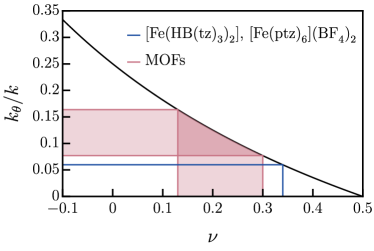
Figure 6: The relationship between Poisson’s ratio, $\nu$, and the ratio of spring constants, $k_{\theta}/k$ in our model, Eq. 35. The blue line shows the measured value of $\nu$ (and corresponding $k_{\theta}/k$) for [Fe(HB(tz)3)2] [65] and [Fe(ptz)6](BF4)2 [70] – the only SCO materials for which $\nu$ has been reported. The pink shaded region indicates typical values of $\nu$ (and hence $k_{\theta}/k$) for MOFs. For isotropic, elastic materials the bulk, shear and Young’s moduli are positive, which implies that $-1/10\leq\nu\leq 1/2$. This requires that $0\leq k_{\theta}/k\leq 1/3$.

Combining the last two results yields

$$\frac{k_{\theta}}{k}=\frac{G}{6B}=\frac{1}{4}\frac{(1-2\nu)}{(1+\nu)},$$ (35)

where $\nu$ is Poisson’s ratio [71]. Typically $0.13\lesssim\nu\lesssim 0.3$ in MOFs [65, 63], and $\nu=0.34$ in the two SCO molecular crystals for which we are aware of measurements – [Fe(HB(tz)3)2] [65] and [Fe(ptz)6](BF4)2 [70], where tz=1,2,4-triazol-1-yl, and ptz=1-propyltetrazole. Thus Eq. (35) yields ${k_{\theta}}/{k}\simeq 0.07-0.17$ for frameworks and ${k_{\theta}}/{k}\simeq 0.06$ for [Fe(HB(tz)3)2] and [Fe(ptz)6](BF4)2. Notice that experiments constrain the ratio ${k_{\theta}}/{k}$ much more tightly than either spring constant.

Typically $2\delta\approx 0.2$ Å for Fe(II) complexes [72, 73] and $2\delta\approx 0.1-0.13$ Å for Fe(III) complexes [74].

Using these values we can estimate the magnitude of the Ising coupling constants; here we choose $\overline{R}=49\delta$ and $\nu=0.13-0.34$. This yields $J_{10}=0.2592$ to $0.1977$ $\delta^{2}k$, $J_{11}/k\delta^{2}=-0.1195$ to $-0.1204$, and $J_{20}/k\delta^{2}=0.1089$ to $0.1333$. Thus, these Ising constants have similar magnitudes. Moreover, $J_{n0}>0$ for any $n$, therefore the first few $J_{n0}$ will induce considerable geometrical frustration in the system. Slichter and Drickamer [21, 15] proposed a simple model for the free energy of a SCO system, where the cooperativity of the system is given by the “cooperativity parameter” $\Gamma$. Rough estimates of $\Gamma$ for our model, considering only nearest neighbour interactions, are within the same order of magnitude as experimental reported values [75, 76].

V Collective behavior: spin-state ordering and transitions

V.1 Devil’s staircase and the zero-temperature phase diagram

Despite containing just three dimensionless parameters $k_{\theta}/k$, $\Delta H/k\delta^{2}$, and $\Delta S/k_{B}$ our model predicts many of the diverse properties observed in the 1$n$02 and 1$n$24 SCO frameworks. We present the zero temperature phase diagram of the resultant Ising model in Fig. 7. To construct this diagram we introduced a cut-off distance, $n_{\text{max}}=m_{\text{max}}=30$, with all Ising coupling constants beyond this cut-off set to zero. We solve the Ising model, Eq. (30), quasianalytically at $T=0$, by considering different states found using Metropolis Monte Carlo simulations at $T>0$, we also consider states similar in structure to the states found using Monte Carlo, and states previously observed in SCO frameworks [31]. The considered states have a maximum unit cell size of $31\times 31$ sites. The $T=0$ phase is then set to be the state with the lowest energy.

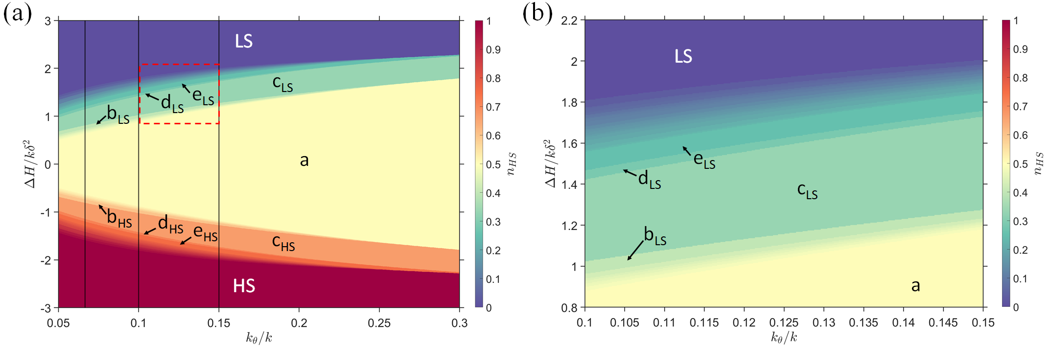
Figure 7: Zero temperature phase diagram of the Ising model derived from the elastic model. The letters indicate selected orders shown in Fig. 8. The dashed red square indicates the region of the phase diagram depicted in (b), where we show in more detail the variety of spin-state phases produced by our model. The three most prominent phases: HS, LS and Néel order (labeled $a$) are observed in many materials in the 1$n$02 and 1$n$24 families of frameworks [31, 34, 42, 35, 43, 44, 45, 46, 47, 48, 49, 50, 51, 52, 53]. The only other antiferroelastic order that has been reported in these families, to date [31], are width 2:1 [34, 51, 46] and 3:1 diagonal stripes [53, 47, 49, 50]. These phases are labeled $c_{\text{LS/HS}}$ and $e_{\text{LS/HS}}$ respectively, where the sub-index indicates whether the majority of sites are LS or HS. All five experimentally observed phases are found in the region of the phase diagram indicated by measurements of the bulk and shear moduli (Fig. 6). Thus our theory describes the antiferroelastic phases observed to date. The vertical black lines indicate the $n_{HS}$ curves in the first column in Fig. 9. This diagram was constructed for an infinite lattice with interactions cut off at $n_{\text{max}}=m_{\text{max}}=30$.

The main features of the zero temperature phase diagram can be understood directly from the details of the mapping from the elastic model to the Ising model (detailed in Section III.1). For small $k_{\theta}/k$ many of the Ising coupling constants for near neighbours have comparable magnitudes and opposing tendencies, cf. Fig. 3. This leads to considerable frustration in the system, which, in turn, leads to multiple competing orders. As $k_{\theta}/k$ increases the magnitude of the nearest neighbour Ising coupling, $J_{1,0}$, becomes significantly larger than other Ising couplings, cf. Fig. 4. This reduces the frustration in the system, which leads to the shrinking in width of the intermediate phases between phase a and phases $c_{\text{LS/HS}}$, and between phases $c_{\text{LS/HS}}$ and the LS/HS phases, cf. Fig. 7.

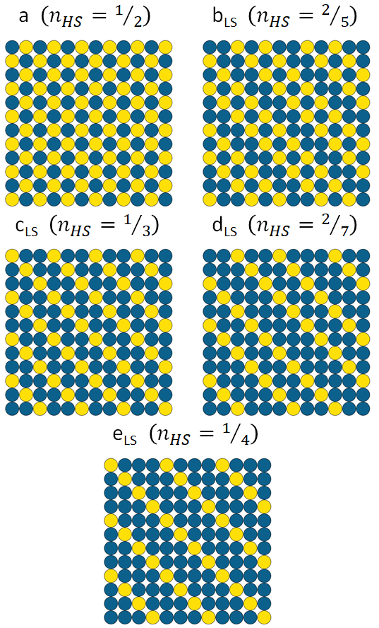
Figure 8: Selected spin-state orderings found in the Ising model at $T=0$ with $n_{\text{max}}=m_{\text{max}}=30$. The labeling corresponds to that in Fig. 7. Where $n_{HS}\neq 1/2$, we include only the LS variant indicated by the sub-index LS. Yellow circles correspond to HS metals and blue to LS metals.

The $a$ phase, commonly known as Néel phase (sometimes called the checkerboard phase in the SCO literature; Fig. 8a), is stable over a wide range of $\Delta H/k\delta^{2}$, and its vertical width in the phase diagram increases as $k_{\theta}/k$ increases. This is consistent with the fact that $J_{1,0}$ is anti-ferromagnetic and increases in magnitude with respect to the other Ising coupling constants as $k_{\theta}/k$ increases, cf. Section III.1. Néel order is commonly found in many materials in the 1$n$02 and 1$n$24 families [31, 34, 42, 35, 43, 44, 45, 46, 47, 48, 49, 50, 51, 52, 53].

Near the Néel phase we also find diagonal stripe phases of width 2:1 ($n_{HS}=1/3$ or 2/3; Fig. 8c), 3:1:2:1 ($n_{HS}=2/7$ or 5/7; Fig. 8d), and 3:1 ($n_{HS}=1/4$ or 3/4; Fig. 8e). Both the 2:1 stripe [34, 51, 46, 31] and 3:1 stripe [53, 47, 49, 50, 31] phases have been observed in 1$n$24 materials. From experimental measurements of Poisson’s ratio we can directly determine $k_{\theta}/k$ and hence the possible antiferroelastic phases, for realistic values we observe three commonly observed antiferroelastic phases.

We also find another antiferroelastic phase at zero temperature characterized by stripes of alternating width 2:1:1:1 ($n_{HS}=0.4$ or 0.6; Fig. 8b). We are not aware of experimental reports of this phase. In the vicinity of this phase there is a high density of phases close in structure. Similarly, between the $c_{\text{LS/HS}}$ phases and the LS/HS phases we observe a high density of stripe phases where they alternate between HS (upper half of the phase diagram) and LS (lower half of the phase diagram) stripes of width 1, and HS/LS stripes of increasing width as the phases get closer to the HS/LS regions respectively, the periodicity of the bigger stripes varies as well, see for example Figs. 8d and e. Near the regions of high density, phases with aperiodic ordering naturally arise as a result of the coexistence of domains. These phases are close in enthalpy to the ground states, however their higher entropy leads to an entropic favourability at finite temperatures.

Plots of $n_{HS}$ as a function of $\Delta H$ for fixed $k_{\theta}/k$ resemble a Devil’s staircase, see Figs. 1, 9. Although, it is not possible to demonstrate an infinite number of steps in this kind of numerical calculation. To test the validity of these phases we produced phase diagrams with increasing $n_{\text{max}}$, as this value increased the vertical width and position of the mentioned phases converges. Therefore, our results provide strong evidence for Devil’s staircases in this model.

V.2 Hidden Devil’s staircase at non-zero temperatures

To study the finite temperature properties of the model we performed Monte Carlo (MC) simulations using the Metropolis algorithm, and parallel tempering for different combinations of $k_{\theta}/k$, $\Delta H$, and $\Delta S$. Similar cooling-heating calculations are reported in the supplementary material [54]. The simulations were performed on a $60\times 60$ lattice with periodic boundary conditions. We used this lattice size because it is commensurate with many of the phases found in our phase diagram calculations. The Ising coupling constants were calculated from Eq. (II) using a $5\,000\times 5\,000$ Monkhorst-Pack grid, and the cut-off was set to $n_{\text{max}}=m_{\text{max}}=29$ to avoid self-interaction.

We initialized the simulations in a random configuration, we let each temperature equilibrate for $500\times 60\times 60$ single-spin-flip MC steps, then we do $50\times 60\times 60$ single-spin-flip MC steps before attempting to swap spin-configuration between adjacent temperatures; we repeat this process $4\,000$ times. After this we let each temperature run for $40\,000\times 60\times 60$ single-spin-flip MC steps, and for the thermodynamic averages we discarded the first $30\,000\times 60\times 60$ steps. We use parallel tempering to find the lowest free energy states.

We plot the thermal dependence of the fraction of HS metals for different values of $k_{\theta}/k$, $\Delta S$, and $\Delta H$ in Figs. 1, 9 and S5. We observe multi-step transitions, evidenced by multiple plateaus in the fraction of HS metals. Each plateau corresponds to a different phase with a different spin state order, Fig. 8. The size of the $n_{HS}=1/2$ plateau increases as we increase $k_{\theta}/k$, consistent with the zero temperature phase diagram, or as we increase $\Delta S$. As $\Delta S$ increases, for fixed $\Delta H$, the transitions become sharper and the plateaus flatter, and the transition curves better resemble their respective $T=0$ $n_{HS}$ curves, cf. Figs. 1, 9 and S5. For non-zero temperatures the first term in Eq. (30) can be expressed as $\frac{1}{2}(\Delta H-T\Delta S)\sum_{i,j}\sigma_{i,j}=\frac{1}{2}\Delta G\sum_{i,j}\sigma_{i,j}$, where $\Delta G$ is the Gibbs free energy difference; as such, sweeping in temperature is similar to moving vertically through the zero temperature phase diagram at a given $k_{\theta}/k$. The magnitude of $\Delta S$ determines the rate of change of $\Delta G$ as the temperature changes. Therefore, larger $\Delta S$ means that the system moves faster through the phase diagram which has the effect of sharpening the transitions while skipping some in our MC calculations.

$\Delta H$ plays an important role in obtaining clear multi-step transitions; because, increasing $\Delta H$ makes the widths of the transitions larger until they eventually become crossovers [31]. Our model confirms this – compare Figs. 9 and S5.

In general, the $T=0$ curves serve as a reasonable guide to predict the non-zero temperature behaviour; the more plateaus above and below the $n_{HS}=1/2$ plateau we observe in the zero-temperature simulations the more gradual the transitions become in the non-zero temperature simulations, in both parallel tempering and cooling-heating. This is a consequence of the high density of spin states in the corresponding parameter space of the phase diagram. These phases are close in energy and in structure, which leads to the appearance of mixed spin-state phases. It is also important to consider the size of the system used in the simulations, as some of the phases in the $T=0$ phase diagram are incommensurate with the size used in this paper, this could also lead to the appearance of mixed phases.

Furthermore, our model is not only relevant for SCO systems, in the context of binary alloys, Frastl and Penrose [32] presented a model where the sites of a 2D square lattice is occupied by either an atom of type A or type B; nearest and next nearest atoms are connected via springs, and the preferred lengths of the springs depend on the types of the connected atoms. They obtained an Ising-like effective Hamiltonian by integrating out mechanical fluctuations. Freschette, Dellago, and Geissler [33, 58] studied a similar model in the context of of lattice mismatch in heterogeneous solids.

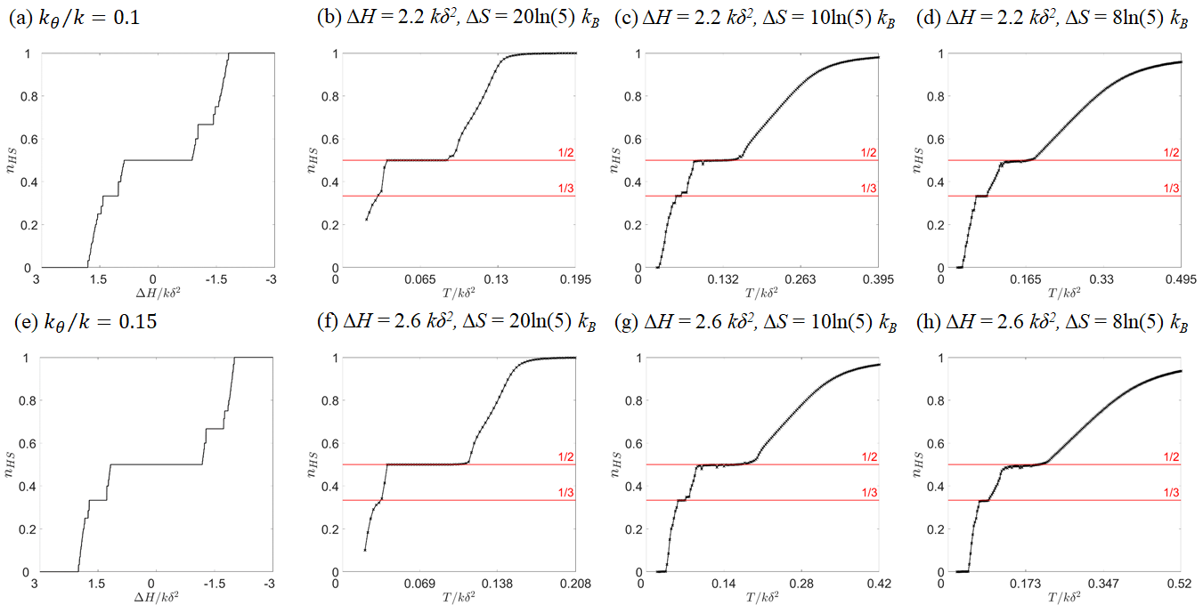
Figure 9: Fraction of HS metals, $n_{HS}$ for different $k_{\theta}/k$, $\Delta H$, and $\Delta S$. From left to right, the first column correspond to the zero temperature $n_{HS}$ curves as indicated by the vertical lines in Fig. 7. To the right we present the parallel tempering simulations with the same $k_{\theta}/k$ as the first curve in a given row. For a given $k_{\theta}/k$, we fix $\Delta H$ and only vary $\Delta S$. For the same set of parameters but higher $\Delta H$ refer to Fig. S5. From left to right the value of $\Delta S$ decreases, and from top to bottom the value of $k_{\theta}/k$ increases. As $\Delta S$ increases, the transitions become sharper and the plateaus flatter, and the transition curves better resemble their respective $T=0$ $n_{HS}$ curves. The size of the $n_{HS}=1/2$ plateau increases as we increase $k_{\theta}/k$, and we observe fewer plateaus and the transitions become less gradual. The horizontal lines indicate the fraction of HS metals for the phases with the largest areas in the $T=0$ phase diagram when $\Delta H>0$, Fig. 7, and with the orderings shown in Fig. 8. We observe that the most noticeable plateaus are the ones corresponding to these phases, consistent with experiments [31].

VI Conclusions

Our two main results are the following. (1) We have shown that there is an exact mapping, based on the displaced oscillator transformation, between elastic and Ising models of SCO materials. We have shown this explicitly for a particular model on the square lattice, but our approach can be extended to other elastic models and geometries. (2) We have shown that for a simple elastic model on the square lattice the long-range Ising interactions lead to a Devil’s staircase in the fraction of HS metals, $n_{HS}$, as the enthalpy difference between spin states, $\Delta H$, is varied at $T=0$. A hidden staircase can also be observed by varying the temperature at fixed $\Delta H$, which corresponds to a single material.

The Ising model has both short-range and long-range interactions. The degree of geometrical frustration in the short-range Ising interactions depends strongly on the relative cost of bending and stretching, $k_{\theta}/k$. For large $k_{\theta}/k$ nearest neighbour interactions dominate. As $k_{\theta}/k$ decreases the other near neighbor interactions become important and the system becomes geometrically frustrated.

At large distances the Ising interactions follow a power law (inverse square law for the square lattice model). This will have important implications for the emergent physics of SCO materials. For example, spin-state ices may be more stable than previously expected [59, 60].

The Ising interactions arise from the elastic potential alone and not from the dynamical behaviors of the phonons. This means that the Ising interactions are not altered by isotopic substitutions and changes in the behavior of SCO materials upon isotopic substitution (see Appendix B) are caused by changes in the single ion physics – specifically $\Delta H$ (due to variations in the zero point energy) and $\Delta S$ (which is dominated by the difference in the vibrational entropy between the two spin-states).

Although our model is purely classical, it is straightforward to extend the calculation to a quantum treatment of phonons, yielding precisely the same Ising model as the classical calculation. The quantum treatment might tempt one to ascribe the Ising interaction to the exchange of virtual phonons [37]. This would be incorrect.

Angular interactions are needed in this model to obtain non-zero Ising couplings. This is because spin-state cooperativity is linked to the inability of the lattice to accommodate the change in geometry associated with a spin state change [29]. Without angular interactions the lattice can accommodate the geometry change at no energetic cost. That is, the angular interactions introduce elastic frustration into the model. Other interactions that lead to elastic frustration, such as second nearest neighbor spring constants [62, 28] could also be included related models to similar effect. Note that elastic frustration in the balls and springs model is logically distinct from and does not imply geometrical frustration in the Ising model. The need for elastic frustration to obtain non-zero Ising couplings leads to a key structure-property relation: in order to develop complex behaviours the lattice needs to have both strong elastic interactions and be flexible enough to accommodate the molecular distortions.

The relationship between Poisson’s ratio, $\nu$, and $k_{\theta}/k$ [Eq. (35)] allows us to relate the mechanical properties of materials to their SCO behaviour. As $\nu\rightarrow 0.5$ the Ising coupling constants go to zero and only crossovers are observed. Thus, we predict that controlling Poisson’s ratio, or equivalently the ratio of the bulk and shear moduli is a key route to engineering emergent phases and multiple antiferroelastic phases in SCO materials.

The high porosity and tunable composition of MOFs provide many ways of engineering multi-step transitions. Experimentally, it has been observed that the addition of guests molecules [47, 49, 77], the postsynthetic modification of ligands [46], and the modification of linkers between SCO centres [78, 77] can change the number of steps in SCO transitions and the order observed at intermediate plateaus. Our work suggests that the key mechanisms by which these modifications act is via modifying the rigidity and ligand field environment of the material.

The explicit model we discuss is relevant to the 1$n$02 and 1$n$24 families of SCO frameworks. It is simple enough to be parameterized from standard experiments (measurements of the bulk and shear moduli, heat capacity, and the crystal structure). Despite the simplicity of our model we are able to reproduce experimentally observed antiferroelastic orderings in the 1$n$02 and 1$n$24 frameworks using typical parameters. In particular, we find prominent multistep transitions and Néel spin-state order at $n_{HS}=1/2$ and diagonal stripes at other intermediate plateaus.

At zero temperature sweeping $\Delta H$ results in a Devil’s staircase in $n_{HS}$, with steps of variable width and pronounced plateaus at $n_{HS}=2/3$, $1/2$, and $1/3$. At finite temperature the Devil’s staircase is partially hidden; nevertheless multi-step transitions with noticeable plateaus at $n_{HS}=1/2$ and $1/3$ remain. However, only a finite number of plateaus survive at finite temperature, as is also found in other Devil’s staircases in statistical mechanical problems [5]. The number of remnant plateaus is strongly correlated with the temperature where half of the metals are HS, $T_{1/2}=\Delta H/\Delta S$. More plateaus remain for either small $\Delta S$ or large $\Delta H$. Thus, we predict that more phases should be evident for materials with a lower $T_{1/2}$.

Applications of our mapping from elastic to Ising models for different geometries and to more detailed elastic models will allow for the study of the effect that structure has on SCO transitions, and how the strength of the interactions and the volume change of the SCO molecules influence hysteresis and spin ordering.

Finally, our model is not only relevant for SCO systems, as it could be applied to any binary system with lattice mismatch. For example, elastic models have been shown to be relevant to the understanding of heterogeneous solids (e.g., binary alloys) [32, 33]. Thus, our work suggests the possibility of Devil’s staircases in such systems.

Appendix A Independence of the Ising coupling constants from lattice dynamics

The Ising coupling constants arise purely from the interactions between metals and ligands, and do not depend on the dynamics of the system. To see this consider the mass weighted Fourier transform

$$u^{(\alpha)}_{\nu,i}(t)=\frac{1}{\sqrt{N}}\sum_{\bm{q}}\frac{1}{\sqrt{m_{\nu}}}e^{i\bm{q}\cdot\bm{R}_{i}}\tilde{u}^{(\alpha)}_{\nu,\bm{q}}e^{-i\omega_{\bm{q}}t}$$ (36)

where we have made the time dependence of $u^{(\alpha)}_{\nu,i}$ explicit. Using Hamilton’s equations of motion on $H_{u}$ we arrive to the eigenvalue problem

$$\omega_{\bm{q}}^{2}\tilde{\bm{\psi}}_{\bm{q}}=\mathcal{D}_{\bm{q}}\tilde{\bm{\psi}}_{\bm{q}},$$ (37)

where $\tilde{\bm{\psi}}_{\bm{q}}$ is a column vector whose elements are $\tilde{\psi}^{(\alpha)}_{\nu,\bm{q}}$, the dynamical matrix, $\mathcal{D}_{\bm{q}}$, is a square matrix whose elements, $d^{\alpha,\alpha^{\prime}}_{\nu,\nu^{\prime},\bm{q}}$, are related to the Hessian by

$$d^{\alpha,\alpha^{\prime}}_{\nu,\nu^{\prime},\bm{q}}=\frac{\mathrm{f}^{\alpha,\alpha^{\prime}}_{\nu,\nu^{\prime},\bm{q}}}{\sqrt{m_{\nu}m_{\nu^{\prime}}}}.$$ (38)

Using the eigenvectors of $\mathcal{D}_{\bm{q}}$ as our basis we can write $H_{u}$ in the form

$$H_{u} = \frac{1}{2}\sum_{\mu,\bm{q}}\left(P_{\mu,\bm{q}}P_{\mu,-\bm{q}}+\omega_{\mu,\bm{q}}^{2}Q^{\prime}_{\mu,\bm{q}}Q^{\prime}_{\mu,-\bm{q}}\right),$$ (39)

where we identify $Q^{\prime}_{\mu,\bm{q}}$ as the normal coordinate for the collective mode $\mu\bm{q}$, $\mu$ enumerates the eigenvalues/vectors of $\mathcal{D}_{\bm{q}}$, and

$$P_{\mu,\bm{q}}=\dot{Q^{\prime}}^{*}_{\mu,\bm{q}},$$ (40)

furthermore, we have

$$H_{u\sigma}=\sum_{\mu,\bm{q}}\xi^{\prime}_{\mu}(\bm{q})Q^{\prime}_{\mu,\bm{q}}\sigma_{-\bm{q}}.$$ (41)

After applying the displaced coordinate transformation, we arrive to the expressions

$$H_{v} = \frac{1}{2}\sum_{\mu,\bm{q}}\left[P_{\mu,\bm{q}}P_{\mu,-\bm{q}}+\omega_{\mu,\bm{q}}^{2}v^{\prime}_{\mu,\bm{q}}v^{\prime}_{\mu,-\bm{q}}\right]$$ (42)

$$H_{\sigma\sigma} = -\frac{1}{2}\sum_{\mu,\bm{q}}\frac{|\xi^{\prime}_{\mu}(\bm{q})|^{2}}{\omega_{\mu,\bm{q}}^{2}}\sigma_{\bm{q}}\sigma_{-\bm{q}}.$$ (43)

where as $N\rightarrow\infty$

$$J_{n}=-\frac{\Omega}{(2\pi)^{d}}\int_{BZ}d^{d}\bm{q}\sum_{\mu}\frac{|\xi^{\prime}_{\mu}(\bm{q})|^{2}}{\omega_{\mu,\bm{q}}^{2}}e^{i\bm{q}\cdot(\bm{R}_{i}-\bm{R}_{i+n})}.$$ (44)

We have used two distinct bases, the eigenvectors of the Hessian (Eq. (II)) and the eigenvectors of the dynamical matrix (Eq. (44)), to yield expressions of $J_{n}$. The dynamical matrix basis makes the masses of the ligands and metals appear explicitly on the expression of $J_{n}$. However, the two expressions must be equal. Therefore, the Ising coupling constants obtained using the mass dependent basis (dynamical matrix) are equal to the Ising coupling constants obtained with the mass independent basis (Hessian matrix) and the Ising coupling constants do not depend on the masses of the constituents of the system. Similarly, the Ising coupling constants cannot depend on the dynamics of the system. This is confirmed numerically, Fig. 10.

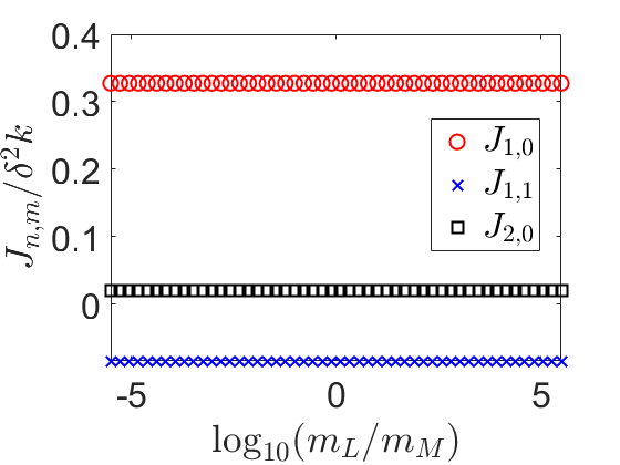
Figure 10: $J_{1,0}$, $J_{1,1}$, and $J_{2,0}$, calculated using the dynamical matrix basis, as a function of $m_{L}$. It can be seen that the Ising coupling constants do not depend on the masses of the ligands and the metals, and are independent on the dynamics of the system. Here $k_{\theta}=k$, but equivalent results are found for other $k_{\theta}/k$.

This allows us to write $H_{v}$ using the dynamical matrix basis and $H_{\sigma\sigma}$ using the Hessian basis, such that

$$\begin{split}H_{v}+H_{\sigma\sigma}=\frac{1}{2}\sum_{\mu,\bm{q}}\left[P_{\mu,\bm{q}}P_{\mu,-\bm{q}}+\omega_{\mu,\bm{q}}^{2}v^{\prime}_{\mu,\bm{q}}v^{\prime}_{\mu,-\bm{q}}\right]\\ -\frac{1}{2}\sum_{\mu,\bm{q}}\frac{|\xi_{\mu}(\bm{q})|^{2}}{\kappa_{\mu,\bm{q}}}\sigma_{\bm{q}}\sigma_{-\bm{q}}.\end{split}$$ (45)

In the context of collective Jahn-Teller transitions in transition metal spinels, Kanamori [37], used displaced operators to transform to new phonon operators. This method yields an expression of the same form as Eq. (43) [38, 79], where the intermolecular interaction was attributed to the exchange of virtual phonons. In our model this might appear to be also the case, but the Hessian basis shows that the interaction is not dynamical in origin. This has the important implication that isotopic substitution will not change the Ising interactions. However, isotopic substitution will change $\Delta H$ (via structural changes) and $\Delta S$ (because this arises predominately from difference vibrational frequencies in the two spin states), see B.

As with the calculation of Ising coupling constants from the Hessian matrix, resolving the $J_{nm}$ into the contributions from individual phonons does not provide any clear insight into their origin. In fact, the phonon basis is even worse than the Hessian basis as the contributions of the individual modes (Fig. S3) depend on the masses of the components even though their sum, Fig. 10, does not!

Appendix B Effects of isotope substitution on spin-state transitions

Isotopic substitution has provided significant insights into molecular and solid state physics. It involves substitution of particular atoms in a compound by the same chemical element with a different nuclear mass (i.e., a nuclear isotope). An example is hydrogen/deuterium substitution which has shown the significant role that quantum nuclear motion can play in hydrogen bonding, particularly in strong hydrogen bonds (see Ref. 80 and references therein). Of particular relevance to the discussion below is that isotopic substitution does not only change vibrational frequencies but can also change bond lengths.

A key piece of evidence on the road to the BCS theory of superconductivity in 1957 was the observation of an isotope effect. In 1950 a shift in the transition temperature of mercury was observed, suggesting that superconductivity resulted from electron-phonon interactions, as argued by Fröhlich that same year. In particular, the magnitude of the shift was consistent with theoretical work by Fröhlich. (Whether he predicted or postdicted the observed effect is a matter of debate, as discussed by Hirsch[81]). BCS theory gives that $\Delta T_{c}/T_{c}=-{1\over 2}\Delta M/M$, which arises from the fact that phonon frequencies scale with $1/\sqrt{M}$ consistent with the mercury experiments. However, in the 1960s there were many observations of “anomalous” isotope effects, particularly in transition metals, that were inconsistent with the prefactor in this equation. These anomalies were resolved by going beyond the BCS theory, and allowing for strong-coupling effects. Following the discovery of cuprate superconductors in 1986, many isotope effects were observed [82] . However, the consensus now is that these observations do not support an electron-phonon mechanism for superconductivity but rather are due to structural changes due to the isotope substitution. For example, isotopic substitution changes the zero-point energy, and that can alter the unit cell volume and the hopping parameter in a Hubbard model.

This history illustrates the subtleties in interpreting isotope experiments. This is because there are both static and dynamical isotope effects. Changes in isotope can lead to changes in structure, such as bond lengths or lattice constants, and even in changes in crystal symmetry. These structural changes arise because the equilibrium structure of the system is that which minimises the total energy of the system. The contribution to this energy from the zero-point energy of the atomic vibrations changes with isotope substitution. Static effects might be classified as those that result from these structural changes. Dynamical effects are those that result from the direct changes in vibrational frequencies.

We now review some of the isotope substitution experiments have been performed on spin-crossover materials. [83, 84, 85, 52, 86] The first studies are reviewed in Section 2.3.5 of Ref. 16. Isotopic exchange was investigated for a tris(picolylamine)iron(II) system which exhibits a two-step transition, suggesting anti-ferro Ising interactions. Significant changes in the spin-state transition curve were observed only when the isotopic substitution (H/D and ¹⁴N/¹⁵N) was made for atoms directly involved in the hydrogen bonding network that connects the spin-crossover molecules. For example, with C₂H₅OD/ND₂ the crossover temperature was shifted to higher temperatures by about 15 K and the middle step was no longer present.

Hosoya et al. [83] studied the two-dimensional coordination polymer spin-crossover compound Fe(pyridine)₂[Ni(CN)₄] and its analogues with the H and N in the pyridine substituted with D and ¹⁵N, respectively. For both isotope substitutions the spin transition temperature decreased by about 10 K, and the hysteresis width changed little. Deuteration decreased the value of $\Delta H$ and $\Delta S$ (determined from differential scanning calorimetry) by about fifteen and ten percent, respectively. The corresponding decreases for N isotope substitution were about ten and six percent (See Table 1 in Ref. 83). Later, Hosoya et al. [84] studied a two-dimensional Hofmann-type clathrate host, Fe(4,4’-bipyridine)Ni(CN)₄·$n$H₂O, with ethanol or acetone guest molecules. In the absence of guests the complex did not exhibit a spin-state transition. Introduction of ethanol and acetone, led to two-step and one-step spin state transitions, respectively. Deuterium substitutions in the guest molecules changed the transition temperatures and transition widths by amounts of the order of 10 K.

Weber et al. [86], studied the iron(II) spin-crossover complex [FeL1(HIm)₂] and its isotopic deuterium-labelled analogue [FeL1(DIm)₂] where HIm is imidazole. Both exhibit a single-step transition with hysteresis. H/D exchange decreased both the transition temperature and the hysteresis width by a few K. Deuteration decreased the value $\Delta H$ and $\Delta S$ (determined from differential scanning calorimetry) by about twenty and ten percent, respectively. (See Table 2 in Ref. 86). They estimated an interaction parameter $J=560$ K, indicating strong intermolecular interactions, which they attributed to a hydrogen bond involving an oxygen atom of the Schiff base like ligand that serves as a donor for the iron centre. They reference some earlier studies showing how the magnitude of the ligand field in a transition metal complex can be modified by hydrogen bonds involving the complex.

Kosone et al. [52] studied a framework material where in the pyridine ligands hydrogen was substituted with deuterium or nitrogen with ¹⁵N. Both substitutions led to significant changes in the shape of the curve describing the temperature dependence of the fraction of high spin molecules. Such a change can occur due to a change in the relative magnitude of $\Delta S$.

Very recently, Jornet-Mollá et al. [85] studied the iron(II) salt [Fe(bpp)₂](isonicNO)₂·HisonicNO·5H₂O, which with decreasing temperature undergoes a transition at 162 K. There is a width of about 5 K, associated with hysteresis. With deuteration the transition temperature decreases to 155 K, the width increases to 7 K, and the enthalpy and entropy changes both increase by about fifteen percent.

In terms of an Ising model picture, the crossover temperature is given by $T_{1/2}=\Delta H/\Delta S$ and the presence of hysteresis and the difference between the transition temperature for increasing and decreasing temperature sweeps is determined by the magnitude of $J$. The results in Appendix A imply that there should be no dynamical isotope effects on the $J$’s, i.e. the inter-spin interactions. This does not rule out changes in the crossover temperature $T_{1/2}=\Delta H/\Delta S$. Both $\Delta H$ and $\Delta S$ can change with isotope substitution. The former due to change in zero-point energies, and the latter due to changes in the vibrational contribution to the entropy change.

References

- Bak [1986] P. Bak, The devil’s staircase, Phys. Today 39, 38 (1986).
- Bak [1982] P. Bak, Commensurate phases, incommensurate phases and the devil’s staircase, Reports on Progress in Physics 45, 587 (1982).
- Thomson et al. [2001] B. Thomson, J. Bruckner, and A. Bruckner, Elementary Real Analysis (Prentice-Hall, 2001).
- Bass [2013] R. Bass, Real Analysis for Graduate Students (Createspace Ind Pub, 2013).
- Bak and von Boehm [1980] P. Bak and J. von Boehm, Ising model with solitons, phasons, and “the devil’s staircase”, Phys. Rev. B 21, 5297 (1980).
- Selke [1988] W. Selke, The annni model — theoretical analysis and experimental application, Physics Reports 170, 213 (1988).
- Yeomans [1988] J. Yeomans, The theory and application of axial ising models (Academic Press, 1988) pp. 151–200.
- Bak and Bruinsma [1982] P. Bak and R. Bruinsma, One-dimensional Ising model and the complete Devil’s staircase, Phys. Rev. Lett. 49, 249 (1982).
- Trzop et al. [2016] E. Trzop, D. Zhang, L. Piñeiro-Lopez, F. J. Valverde-Muñoz, C. M. Muñoz, L. Palatinus, L. Guerin, H. Cailleau, J. A. Real, and E. Collet, First step towards a devil’s staircase in spin-crossover materials, Angew. Chem. Int. Ed. 55, 8675 (2016).
- Hauser [2004] A. Hauser, Ligand field theoretical considerations, in Spin Crossover in Transition Metal Compounds I. Topics in Current Chemistry, Vol. 233, edited by P. Gütlich and H. Goodwin (Springer, Berlin, Heidelberg, 2004).
- Cobo et al. [2008] S. Cobo, D. Ostrovskii, S. Bonhommeau, L. Vendier, G. Molnár, L. Salmon, K. Tanaka, and A. Bousseksou, Single-laser-shot-induced complete bidirectional spin transition at room temperature in single crystals of (FeII(pyrazine)(Pt(CN)4)), J. Am. Chem. Soc 130, 9019 (2008).
- Ksenofontov et al. [2004] V. Ksenofontov, A. B. Gaspar, and P. Gütlich, Pressure effect studies on spin crossover and valence tautomeric systems, in Spin Crossover in Transition Metal Compounds III (Springer Berlin Heidelberg, Berlin, Heidelberg, 2004) pp. 23–64.
- Bousseksou et al. [2004] A. Bousseksou, F. Varret, M. Goiran, K. Boukheddaden, and J. P. Tuchagues, The spin crossover phenomenon under high magnetic field, in Spin Crossover in Transition Metal Compounds III (Springer Berlin Heidelberg, Berlin, Heidelberg, 2004) pp. 65–84.
- Prins et al. [2011] F. Prins, M. Monrabal-Capilla, E. A. Osorio, E. Coronado, and H. S. J. van der Zant, Room-temperature electrical addressing of a bistable spin-crossover molecular system, Adv. Mater 23, 1545 (2011).
- Pavlik and Boča [2013] J. Pavlik and R. Boča, Established static models of spin crossover, Eur. J. Inorg. Chem 2013, 697 (2013).
- Gütlich and Goodwin [2004] P. Gütlich and H. A. Goodwin, Spin crossover—an overall perspective, in Spin Crossover in Transition Metal Compounds I, edited by P. Gütlich and H. Goodwin (Springer Berlin Heidelberg, Berlin, Heidelberg, 2004) pp. 1–47.
- Bousseksou et al. [2011] A. Bousseksou, G. Molnár, L. Salmon, and W. Nicolazzi, Molecular spin crossover phenomenon: recent achievements and prospects, Chem. Soc. Rev 40, 3313 (2011).
- Guionneau [2014] P. Guionneau, Crystallography and spin-crossover. a view of breathing materials, Dalton Trans. 43, 382 (2014).
- Mullaney et al. [2017] B. R. Mullaney, L. Goux-Capes, D. J. Price, G. Chastanet, J.-F. Létard, and C. J. Kepert, Spin crossover-induced colossal positive and negative thermal expansion in a nanoporous coordination framework material, Nat. Commun 8 (2017).
- Wajnflasz and Pick [1971] J. Wajnflasz and R. Pick, Transitions “Low Spin”-“High Spin” Dans les complexes de Fe2+, J. Phys. Colloq. 32, C1 (1971).
- Slichter and Drickamer [1972] C. P. Slichter and H. G. Drickamer, Pressure‐induced electronic changes in compounds of iron, J. Chem. Phys 56, 2142 (1972).
- Watanabe et al. [2016] H. Watanabe, K. Tanaka, N. Bréfuel, H. Cailleau, J.-F. m. c. Létard, S. Ravy, P. Fertey, M. Nishino, S. Miyashita, and E. Collet, Ordering phenomena of high-spin/low-spin states in stepwise spin-crossover materials described by the annni model, Phys. Rev. B 93, 014419 (2016).
- Konishi et al. [2008] Y. Konishi, H. Tokoro, M. Nishino, and S. Miyashita, Monte Carlo simulation of pressure-induced phase transitions in spin-crossover materials, Phys. Rev. Lett. 100, 067206 (2008).
- Traiche et al. [2018] R. Traiche, M. Sy, and K. Boukheddaden, Elastic frustration in 1D spin-crossover chains: Evidence of multi-step transitions and self-organizations of the spin states, J. Phys. Chem. C 122, 4083 (2018).
- Nishino et al. [2007] M. Nishino, K. Boukheddaden, Y. Konishi, and S. Miyashita, Simple two-dimensional model for the elastic origin of cooperativity among spin states of spin-crossover complexes, Phys. Rev. Lett. 98, 247203 (2007).
- Nishino et al. [2009] M. Nishino, K. Boukheddaden, and S. Miyashita, Molecular dynamics study of thermal expansion and compression in spin-crossover solids using a microscopic model of elastic interactions, Phys. Rev. B 79, 012409 (2009).
- Enachescu et al. [2012] C. Enachescu, M. Nishino, S. Miyashita, L. Stoleriu, and A. Stancu, Monte Carlo Metropolis study of cluster evolution in spin-crossover solids within the framework of a mechanoelastic model, Phys. Rev. B 86, 054114 (2012).
- Paez-Espejo et al. [2016] M. Paez-Espejo, M. Sy, and K. Boukheddaden, Elastic frustration causing two-step and multistep transitions in spin-crossover solids: Emergence of complex antiferroelastic structures, J. Am. Chem. Soc 138, 3202 (2016).
- Halcrow [2011] M. A. Halcrow, Structure:function relationships in molecular spin-crossover complexes, Chem. Soc. Rev 40, 4119 (2011).
- Halcrow [2014] M. A. Halcrow, Spin-crossover compounds with wide thermal hysteresis, Chem. Lett 43, 1178 (2014).
- Cruddas and Powell [2020a] J. Cruddas and B. J. Powell, Structure–property relationships and the mechanisms of multistep transitions in spin crossover materials and frameworks, Inorg. Chem. Front. 7, 4424 (2020a).
- Fratzl and Penrose [1995] P. Fratzl and O. Penrose, Ising model for phase separation in alloys with anisotropic elastic interaction—I. Theory, Acta Metall. Mater. 43, 2921 (1995).
- Frechette et al. [2019] L. B. Frechette, C. Dellago, and P. L. Geissler, Consequences of lattice mismatch for phase equilibrium in heterostructured solids, Phys. Rev. Lett. 123, 135701 (2019).
- Ortega-Villar et al. [2016] N. Ortega-Villar, M. Muñoz, and J. Real, Symmetry breaking in iron(II) spin-crossover molecular crystals, Magnetochemistry 2, 16 (2016).
- Halder et al. [2002] G. J. Halder, C. J. Kepert, B. Moubaraki, K. S. Murray, and J. D. Cashion, Guest-dependent spin crossover in a nanoporous molecular framework material, Science 298, 1762 (2002).
- Ni et al. [2017] Z.-P. Ni, J.-L. Liu, M. N. Hoque, W. Liu, J.-Y. Li, Y.-C. Chen, and M.-L. Tong, Recent advances in guest effects on spin-crossover behavior in Hofmann-type metal-organic frameworks, Coord. Chem. Rev. 335, 28 (2017).
- Kanamori [1960] J. Kanamori, Crystal distortion in magnetic compounds, J. Appl. Phys 31, S14 (1960).
- Gehring and Gehring [1975] G. A. Gehring and K. A. Gehring, Co-operative Jahn-Teller effects, Rep. Prog. Phys 38, 1 (1975).
- Boukheddaden et al. [2007] K. Boukheddaden, S. Miyashita, and M. Nishino, Elastic interaction among transition metals in one-dimensional spin-crossover solids, Phys. Rev. B 75, 094112 (2007).
- Bolvin and Kahn [1995] H. Bolvin and O. Kahn, Ising model for low-spin high-spin transitions in molecular compounds; within and beyond the mean-field approximation, Chem. Phys 192, 295 (1995).
- Monkhorst and Pack [1976] H. J. Monkhorst and J. D. Pack, Special points for Brillouin-zone integrations, Phys. Rev. B 13, 5188 (1976).
- Adams et al. [2011] C. J. Adams, M. C. Muñoz, R. E. Waddington, and J. A. Real, Cooperative spin transition in the two-dimensional coordination polymer [Fe(4,4’-bipyridine)2(NC)2]4CHCl3 = S, Se), Inorg. Chem. 50, 10633 (2011).
- Lin et al. [2012] J.-B. Lin, W. Xue, B.-Y. Wang, J. Tao, W.-X. Zhang, J.-P. Zhang, and X.-M. Chen, Chemical/physical pressure tunable spin-transition temperature and hysteresis in a two-step spin crossover porous coordination framework, Inorg. Chem. 51, 9423 (2012).
- Bao et al. [2012] X. Bao, P.-H. Guo, W. Liu, J. Tucek, W.-X. Zhang, J.-D. Leng, X.-M. Chen, I. A. Gural’skiy, L. Salmon, A. Bousseksou, and M.-L. Tong, Remarkably high-temperature spin transition exhibited by new 2D metal–organic frameworks, Chem. Sci. 3, 1629 (2012).
- Halder et al. [2008] G. J. Halder, K. W. Chapman, S. M. Neville, B. Moubaraki, K. S. Murray, J.-F. Létard, and C. J. Kepert, Elucidating the mechanism of a two-step spin transition in a nanoporous metal-organic framework, J. Am. Chem. Soc. 130, 17552 (2008).
- Clements et al. [2016] J. E. Clements, J. R. Price, S. M. Neville, and C. J. Kepert, Hysteretic four-step spin crossover within a three-dimensional porous Hofmann-like material, Angew. Chem. Int. Ed. 55, 15105 (2016).
- Zhang et al. [2019] C.-J. Zhang, K.-T. Lian, G.-Z. Huang, S. Bala, Z.-P. Ni, and M.-L. Tong, Hysteretic four-step spin-crossover in a 3D Hofmann-type metal–organic framework with aromatic guest, Chem. Commun. 55, 11033 (2019).
- Agustí et al. [2008] G. Agustí, M. C. Muñoz, A. B. Gaspar, and J. A. Real, Spin-crossover behavior in cyanide-bridged iron(II)-gold(I) bimetallic 2D Hofmann-like metal-organic frameworks, Inorg. Chem. 47, 2552 (2008).
- Zhang et al. [2020] C.-J. Zhang, K.-T. Lian, S.-G. Wu, G.-Z. Huang, Z.-P. Ni, and M.-L. Tong, The substituent guest effect on four-step spin-crossover behaviors, Inorg. Chem. Front. 4, 911 (2020).
- Liu et al. [2017] W. Liu, Y.-Y. Peng, S.-G. Wu, Y.-C. Chen, M. N. Hoque, Z.-P. Ni, X.-M. Chen, and M.-L. Tong, Guest-switchable multi-step spin transitions in an amine-functionalized metal–organic framework, Angew. Chem. Int. Ed. 56, 14982 (2017).
- Agustí et al. [2009] G. Agustí, A. B. Gaspar, M. C. Muñoz, P. G. Lacroix, and J. A. Real, Spin crossover and paramagnetic behaviour in two-dimensional iron(II) coordination polymers with stilbazole push–pull ligands, Aust. J. Chem. 62, 1155 (2009).
- Kosone et al. [2008] T. Kosone, C. Kachi-Terajima, C. Kanadani, T. Saito, and T. Kitazawa, Isotope effect on spin-crossover transition in a new two-dimensional coordination polymer [FeII(C5H5N)2][AuI(CN)2]2, [FeII(C5D5N)2][AuI(CN)2]2, and [FeII(C5H515N)2][AuI(CN)2]2, Chem. Lett. 37, 422 (2008).
- Meng et al. [2017] Y. Meng, Q. Sheng, M. N. Hoque, Y. Chen, S. Wu, J. Tucek, R. Zboril, T. Liu, Z. Ni, and M. Tong, Two-step spin-crossover with three inequivalent FeII sites in a two-dimensional Hofmann-type coordination polymer, Chem. Eur. J. 23, 10034 (2017).
- [54] See Supplemental Material at [URL will be inserted by publisher] for calculation of the shear modulus, decomposition of the Ising constants into different modes, and additional Monte Carlo calculations.
- Nakada et al. [2011] T. Nakada, P. A. Rikvold, T. Mori, M. Nishino, and S. Miyashita, Crossover between a short-range and a long-range Ising model, Phys. Rev. B 84, 054433 (2011).
- Nakada et al. [2012] T. Nakada, T. Mori, S. Miyashita, M. Nishino, S. Todo, W. Nicolazzi, and P. A. Rikvold, Critical temperature and correlation length of an elastic interaction model for spin-crossover materials, Phys. Rev. B 85, 054408 (2012).
- Miyashita et al. [2008] S. Miyashita, Y. Konishi, M. Nishino, H. Tokoro, and P. A. Rikvold, Realization of the mean-field universality class in spin-crossover materials, Phys. Rev. B 77, 014105 (2008).
- Frechette et al. [2020] L. B. Frechette, C. Dellago, and P. L. Geissler, Origin of mean-field behavior in an elastic ising model, Phys. Rev. B 102, 024102 (2020).
- Cruddas and Powell [2019] J. Cruddas and B. J. Powell, Spin-state ice in elastically frustrated spin-crossover materials, J. Am. Chem. Soc 141, 19790 (2019).
- Cruddas and Powell [2020b] J. Cruddas and B. J. Powell, Multiple Coulomb phases with temperature tunable ice rules in pyrochlore spin crossover materials, arXiv:2007.13983 (2020b).
- Castelnovo et al. [2012] C. Castelnovo, R. Moessner, and S. Sondhi, Spin ice, fractionalization, and topological order, Annu. Rev. Condens. Matter Phys. 3, 35 (2012).
- Ye et al. [2015] H.-Z. Ye, C. Sun, and H. Jiang, Monte-Carlo simulations of spin-crossover phenomena based on a vibronic Ising-like model with realistic parameters, Phys. Chem. Chem. Phys. 17, 6801 (2015).
- Tan and Cheetham [2011] J. C. Tan and A. K. Cheetham, Mechanical properties of hybrid inorganic–organic framework materials: establishing fundamental structure–property relationships, Chem. Soc. Rev 40, 1059 (2011).
- Spencer et al. [2009] E. C. Spencer, R. J. Angel, N. L. Ross, B. E. Hanson, and J. A. K. Howard, Pressure-induced cooperative bond rearrangement in a zinc imidazolate framework: A high-pressure single-crystal X-ray diffraction study, J. Am. Chem. Soc 131, 4022 (2009).
- Mikolasek et al. [2018] M. Mikolasek, M. D. Manrique-Juarez, H. J. Shepherd, K. Ridier, S. Rat, V. Shalabaeva, A.-C. Bas, I. E. Collings, F. Mathieu, J. Cacheux, T. Leichle, L. Nicu, W. Nicolazzi, L. Salmon, G. Molnár, and A. Bousseksou, Complete set of elastic moduli of a spin-crossover solid: Spin-state dependence and mechanical actuation, J. Am. Chem. Soc 140, 8970 (2018).
- Burtch et al. [2018] N. C. Burtch, J. Heinen, T. D. Bennett, D. Dubbeldam, and M. D. Allendorf, Mechanical properties in metal–organic frameworks: Emerging opportunities and challenges for device functionality and technological applications, Adv. Mater 30, 1704124 (2018).
- Bennett et al. [2017] T. D. Bennett, A. K. Cheetham, A. H. Fuchs, and F.-X. Coudert, Interplay between defects, disorder and flexibility in metal-organic frameworks, Nature Chem 9, 11 (2017).
- Lee et al. [2016] S. J. Lee, C. Doussot, A. Baux, L. Liu, G. B. Jameson, C. Richardson, J. J. Pak, F. Trousselet, F.-X. Coudert, and S. G. Telfer, Multicomponent metal–organic frameworks as defect-tolerant materials, Chem. Mater 28, 368 (2016).
- Tan et al. [2012] J.-C. Tan, B. Civalleri, C.-C. Lin, L. Valenzano, R. Galvelis, P.-F. Chen, T. D. Bennett, C. Mellot-Draznieks, C. M. Zicovich-Wilson, and A. K. Cheetham, Exceptionally low shear modulus in a prototypical imidazole-based metal-organic framework, Phys. Rev. Lett. 108, 095502 (2012).
- Jung et al. [1996] J. Jung, F. Bruchhäuser, R. Feile, H. Spiering, and P. Gütlich, Multiple Coulomb phases with temperature tunable ice rules in pyrochlore spin crossover materials, Z. Phys. B 100, 517 (1996).
- Hearn [1997] E. Hearn, Chapter 14 - complex strain and the elastic constants, in Mechanics of Materials 1 (Third Edition), edited by E. Hearn (Butterworth-Heinemann, Oxford, 1997) third edition ed., pp. 361 – 400.
- Collet and Guionneau [2018] E. Collet and P. Guionneau, Structural analysis of spin-crossover materials: From molecules to materials, C R Chim 21, 1133 (2018), spin crossover phenomenon / Phénomène de transition de spin.
- Molnár et al. [2019] G. Molnár, M. Mikolasek, K. Ridier, A. Fahs, W. Nicolazzi, and A. Bousseksou, Molecular spin crossover materials: Review of the lattice dynamical properties, Ann. Phys 531, 1900076 (2019).
- Harding et al. [2016] D. J. Harding, P. Harding, and W. Phonsri, Spin crossover in iron(III) complexes, Coord. Chem. Rev. 313, 38 (2016).
- Roubeau et al. [2011] O. Roubeau, M. Castro, R. Burriel, J. G. Haasnoot, and J. Reedijk, Calorimetric investigation of triazole-bridged Fe(II) spin-crossover one-dimensional materials: Measuring the cooperativity, J. Phys. Chem. B 115, 3003 (2011).
- Linares et al. [1999] J. Linares, H. Spiering, and F. Varret, Analytical solution of 1D Ising-like systems modified by weak long range interaction, Eur. Phys. J. B 10, 271 (1999).
- Valverde-Muñoz et al. [2019] F. J. Valverde-Muñoz, C. Bartual-Murgui, L. Piñeiro-López, M. C. Muñoz, and J. A. Real, Influence of host–guest and host–host interactions on the spin-crossover 3D Hofmann-type clathrates FeII(pina)[MI(CN)2]2·xMeOH (MI = Ag, Au), Inorg. Chem. 58, 10038 (2019).
- Peng et al. [2020] Y.-Y. Peng, S.-G. Wu, Y.-C. Chen, W. Liu, G.-Z. Huang, Z.-P. Ni, and M.-L. Tong, Asymmetric seven-/eight-step spin-crossover in a three-dimensional Hofmann-type metal–organic framework, Inorg. Chem. Front. 7, 1685 (2020).
- Kambara [1981] T. Kambara, Theory of high‐spin low‐spin transitions in transition metal compounds induced by cooperative molecular distortions and lattice strains, J. Chem. Phys 74, 4557 (1981).
- McKenzie et al. [2014] R. H. McKenzie, C. Bekker, B. Athokpam, and S. G. Ramesh, Effect of quantum nuclear motion on hydrogen bonding, J. Chem. Phys. 140, 174508 (2014).
- Hirsch [2011] J. E. Hirsch, Did herbert fröhlich predict or postdict the isotope effect in superconductors?, Physica Scripta 84, 045705 (2011).
- Barbee et al. [1988] T. W. Barbee, M. L. Cohen, L. C. Bourne, and A. Zettl, The isotope and superconducting oxides, J. Phys. C 21, 5977 (1988).
- Hosoya et al. [2003] K. Hosoya, T. Kitazawa, M. Takahashi, M. Takeda, J.-F. Meunier, G. Molnár, and A. Bousseksou, Unexpected isotope effect on the spin transition of the coordination polymer Fe(C5H5N)2[Ni(CN)4], Phys. Chem. Chem. Phys. 5, 1682 (2003).
- Hosoya et al. [2016] K. Hosoya, S.-i. Nishikiori, M. Takahashi, and T. Kitazawa, Spin-crossover behavior of Hofmann-type-like complex Fe(4,4’-bipyridine)Ni(CN)4·nH2O depending on guest species, Magnetochemistry 2, 10.3390/magnetochemistry2010008 (2016).
- Jornet-Mollá et al. [2021] V. Jornet-Mollá, C. Giménez-Saiz, L. Cañadillas-Delgado, D. S. Yufit, J. A. K. Howard, and F. M. Romero, Interplay between spin crossover and proton migration along short strong hydrogen bonds, Chem. Sci. 12, 1038 (2021).
- Weber et al. [2011] B. Weber, W. Bauer, T. Pfaffeneder, M. M. Dîrtu, A. D. Naik, A. Rotaru, and Y. Garcia, Influence of hydrogen bonding on the hysteresis width in iron(II) spin-crossover complexes, Eur. J. Inorg. Chem 2011, 3193 (2011).