Zeros of a table of polynomials satisfying a four-term contiguous relation

Abstract.

For any $A(z),B(z),C(z)\in\mathbb{C}[z]$, we study the zero distribution of a table of polynomials $\left\{P_{m,n}(z)\right\}_{m,n\in\mathbb{N}_{0}}$ satisfying the recurrence relation

$$P_{m,n}(z)=A(z)P_{m-1,n}(z)+B(z)P_{m,n-1}(z)+C(z)P_{m-1,n-1}(z)$$

with the initial condition $P_{0,0}(z)=1$ and $P_{-m,-n}(z)=0$ for all $m,n\in\mathbb{N}$. We show that the zeros of $P_{m,n}(z)$ lie on a curve whose equation is given explicitly in terms of $A(z),B(z)$, and $C(z)$. We also study the zero distribution of a case with a general initial condition.

1. Introduction

The study of the zero distribution of a sequence of polynomials $\left\{S_{N}(z)\right\}_{N\in\mathbb{N}_{0}}$ satisfying a finite recurrence of order $m$

$$\sum_{k=0}^{m}A_{k}(z)S_{N-k}(z)=0,\qquad A_{0}(z)=1,$$

is of interest to many mathematicians. This sequence includes some classical sequences of orthogonal polynomials such as the sequence of Chebyshev polynomials. Orthogonality, in turn, provides information regarding the locations of zeros of polynomials in the sequence (i.e., orthogonality implies reality of zeros). Another approach to find these locations is to use asymptotic analysis and properties of exponential polynomials to obtain an optimal curve containing zeros of all these polynomials (see [4, 5]). In this setting, optimal curve means that the union of all these zeros forms a dense subset of this curve. However, even for the case $m=3$ (four-term recurrence), an explicit equation in terms of the coefficient polynomials, $A_{k}(z)$, for such an optimal curve is still unknown. Some special cases of this four-term recurrence have been studied in [1, 2, 3, 8, 9].

Another approach to the zero distribution of the sequence $\left\{S_{N}(z)\right\}_{N\in\mathbb{N}_{0}}$ is to produce this sequence from a table of polynomials $\left\{P_{m,n}(z)\right\}_{m,n\in\mathbb{N}_{0}}$. This approach necessitates the study of zero distribution of a table of polynomials satisfying a finite recurrence. Motivated by this approach and the unsolved four-term recurrence mentioned above, for $A(z),B(z),C(z)\in\mathbb{C}[z]$, we study the distribution of zeros of a table of polynomials $\left\{P_{m,n}(z)\right\}_{m,n\in\mathbb{N}_{0}}$ satisfying the recurrence relation

$$P_{m,n}(z)+A(z)P_{m-1,n}(z)+B(z)P_{m,n-1}(z)+C(z)P_{m-1,n-1}(z)=0$$

with the standard initial conditions $P_{0,0}(z)=1$ and $P_{-m,-n}(z)=0$ $\forall m,n\in\mathbb{N}$. Equivalently, this table is generated by

(1.1) $$\sum_{m=0}^{\infty}\sum_{n=0}^{\infty}P_{m,n}(z)s^{m}t^{n}=\frac{1}{1+A(z)s+B(z)t+C(z)st}.$$

In the case $A(z)=z$, $B(z)=z$, and $C(z)=z$, the numbers $P_{m,n}(-1)$ are the Delannoy numbers which count the number of nearest-neighbor paths from the origin to $(m,n)$ moving only north, east and northeast (see [6]). When $A(z)=-1$, $B(z)=-1$, and $C(z)=z$, the numbers $P_{m,n}(0)$ are the binomial coefficients ${\displaystyle\binom{m+n}{m,n}=\frac{(m+n)!}{m!n!}}$.

In terms of its connection with the four-term recurrence sequence $\left\{S_{N}(z)\right\}_{N\in\mathbb{N}_{0}}$, letting $t=s^{2}$ in (1.1) produces the sequence $S_{N}(z):=\sum_{m+2n=N}P_{m,n}(z)$ which satisfies the general four-term recurrence

$$S_{N}(z)+A(z)S_{N-1}(z)+B(z)S_{N-2}(z)+C(z)S_{N-3}(z)=0$$

with the initial condition $S_{0}(z)=1$ and $S_{-N}(z)=0$ for $N\in\mathbb{N}$. On the other hand, if we let $t=s$ in (1.1), then with $D(z):=A(z)+B(z)$, we obtain the sequence $R_{N}(z):=\sum_{m+n=N}P_{m,n}(z)$ satisfying the general three-term recurrence

$$R_{N}(z)+D(z)R_{N-1}(z)+C(z)R_{N-2}(z)=0$$

with the same initial condition. The zeros of these polynomials $R_{N}(z)$ which are not zeros of $C(z)$ lie on the curve defined by [7]

$$\Im\frac{D^{2}(z)}{C(z)}=0\qquad\text{and}\qquad 0\leq\Re\frac{D^{2}(z)}{C(z)}\leq 4$$

and are dense there as $N\rightarrow\infty$.

Before stating our theorem, we quickly mention that in the special case $A(z)=1$, $B(z)=1$, and $C(z)=z$, the diagonal of our table $\left\{P_{m,n}(z)\right\}_{m,n\in\mathbb{N}_{0}}$ defined in (1.1) relates to the famous sequence of Legendre polynomials $\left\{L_{m}(z)\right\}_{m=0}^{\infty}$ (c.f. Lemma 4) by

$$P_{m,m}(z)=z^{m}L_{m}\left(\frac{2}{z}-1\right).$$

With $\mathcal{Z}(P_{m,n})$ denoting the set of zeros of $P_{m,n}(z)$, we state our theorem.

Theorem 1.

For any polynomials $A(z),B(z),C(z)\in\mathbb{C}[z]$, let $\left\{P_{m,n}(z)\right\}_{m,n=0}^{\infty}$ be the table of polynomials generated by (1.1). Then for any $m,n\in\mathbb{N}_{0}$, all the zeros of $P_{m,n}(z)$ which satisfy $A(z)B(z)\neq 0$ lie on the curve $\mathcal{C}$ defined by

$$\Im\left(\frac{C(z)}{A(z)B(z)}\right)=0\qquad\text{and}\qquad\Re\left(\frac{C(z)}{A(z)B(z)}\right)\geq 1,$$

and ${\displaystyle\bigcup_{m,n=0}^{\infty}\mathcal{Z}\left(P_{m,n}\right)}$ is dense on $\mathcal{C}$.

We will prove this theorem in Section 2 and study a general initial condition (c.f. Theorem 5) in Section 3. We end the introduction with an example of Theorem 1.

Example.

In the case $A(z)=1$, $B(z)=z^{2}-2z+2$, and $C(z)=z$, we let $z=x+iy$ and compute

$$\Im\left(\frac{C(z)}{A(z)B(z)}\right) =-\frac{y\left(x^{2}+y^{2}-2\right)}{\left((x-1)^{2}+(y-1)^{2}\right)\left((x-1)^{2}+(y+1)^{2}\right)},$$

$$\Re\left(\frac{C(z)}{A(z)B(z)}\right) =\frac{x^{3}-2x^{2}+xy^{2}+2x-2y^{2}}{\left((x-1)^{2}+(y-1)^{2}\right)\left((x-1)^{2}+(y+1)^{2}\right)}.$$

The equation $\Im\left(C(z)/(A(z)B(z))\right)=0$ implies that $\mathcal{C}$ is a portion of the line $y=0$ and a portion of the circle $x^{2}+y^{2}-2=0$. In the case $y=0$, the inequality $\Re\left(C(z)/(A(z)B(z))\right)-1\geq 0$ yields $(x-1)(2-x)\geq 0$. Similarly in the case $x^{2}+y^{2}=2$, this inequality gives

$$\Re\left(\frac{C(z)}{A(z)B(z)}\right)-1=\frac{3-2x}{2(x-1)}\geq 0$$

or equivalently $x\geq 1$ since $3-2x>0$ (for $x^{2}+y^{2}=2$). We conclude that $\mathcal{C}$ is the union of the interval $[1,2]$ and the portion of the circle $x^{2}+y^{2}=2$ with $x\geq 1$ (see Figure 1.1).

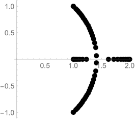
Figure 1.1. Zeros of $P_{50,30}(z)$ when $A(z)=1$, $B(z)=z^{2}-2z+2$, and $C(z)=z$

2. Proof of the theorem

For any $z$ such that $A(z)B(z)\neq 0$, we make the substitutions $s\rightarrow s/A(z)$, $t\rightarrow t/B(z)$ and rewrite (1.1) as

$$\sum_{m=0}^{\infty}\sum_{n=0}^{\infty}P_{m,n}(z)\frac{s^{m}}{A^{m}(z)}\frac{t^{n}}{B^{n}(z)}=\frac{1}{1+s+t+C(z)st/A(z)B(z)}.$$

If we let $\left\{H_{m,n}(z)\right\}_{m,n=0}^{\infty}$ be the table of polynomials generated by

(2.1) $$\sum_{m=0}^{\infty}\sum_{n=0}^{\infty}H_{m,n}(z)s^{m}t^{n}=\frac{1}{1+s+t+zst},$$

then

$$A^{m}(z)B^{n}(z)H_{m,n}\left(\frac{C(z)}{A(z)B(z)}\right)=P_{m,n}(z).$$

Thus to prove 1, it suffices to prove that for any $m,n\in\mathbb{N}_{0}$, the zeros of $H_{m,n}(z)$ lie on $[1,\infty)$ and $\bigcup_{m,n=0}^{\infty}\mathcal{Z}\left(H_{m,n}\right)$ is dense on this interval.

From (2.1), for small $s,t$, we have

$$\sum_{m=0}^{\infty}\sum_{n=0}^{\infty}H_{m,n}(z)s^{m}t^{n} =\frac{1}{1+s+t(1+zs)}$$

$$=\frac{1}{(1+s)\left(1+\frac{1+zs}{1+s}t\right)}$$

$$=\frac{1}{1+s}\sum_{n=0}^{\infty}t^{n}(-1)^{n}\left(\frac{1+zs}{1+s}\right)^{n}$$

$$=\sum_{n=0}^{\infty}t^{n}(-1)^{n}\frac{(1+zs)^{n}}{(1+s)^{n+1}}$$

and consequently for each $n\in\mathbb{N}_{0}$

(2.2) $$\sum_{m=0}^{\infty}H_{m,n}(z)s^{m}=(-1)^{n}\frac{(1+zs)^{n}}{(1+s)^{n+1}}.$$

Lemma 2.

For each fixed $n\in\mathbb{N}_{0}$, let $\left\{Q_{m,n}(z)\right\}_{m\in\mathbb{N}_{0}}$ be the sequence of polynomials generated by

(2.3) $$\sum_{m=0}^{\infty}Q_{m,n}(z)s^{m}=\frac{(1+s)^{n}}{1+zs}.$$

Then

$$Q_{m,n}(z)=\begin{cases}\sum_{k=0}^{m}(-1)^{m+k}\binom{n}{k}z^{m-k}&\text{ if }m<n\\ (-1)^{m}(z-1)^{n}z^{m-n}&\text{ if }m\geq n.\end{cases}$$

Proof.

From (2.3), we have

$$(1+zs)\sum_{m=0}^{\infty}Q_{m,n}(z)s^{m}=(1+s)^{n}.$$

We collect the coefficient of $s^{m}$ of both sides and conclude that

$$zQ_{m-1,n}(z)+Q_{m,n}(z)=\begin{cases}\binom{n}{m}&\text{ if }1\leq m\leq n\\ 0&\text{ if }m>n\end{cases}$$

and the lemma follows from induction by $m$. ∎

From Lemma 2, if $m\geq n$, then the zeros of all the derivatives (of any orders) of $Q_{m,n}(z)$ lie on the interval $[0,1]$ by the Gauss-Lucas theorem. Thus the reciprocals of the zeros of all these derivatives lie on $[1,\infty)$. With this observation, the fact that the zeros of $H_{m,n}(z)$ lie on $[1,\infty)$ follows from the lemma below.

Lemma 3.

For any $m,n\in\mathbb{N}_{0}$,

$$H_{m,n}(z)=\frac{z^{m}}{n!}Q_{m+n,n}^{(n)}\left(\frac{1}{z}\right),$$

where $Q_{m+n,n}^{(n)}(1/z)$ is the $n$-th derivative of $Q_{m+n,n}(z)$ evaluated at $1/z$ .

Proof.

We compute the $n$-th derivative of both sides of (2.3) in $z$ and obtain

$$\sum_{m=0}^{\infty}Q_{m,n}^{(n)}(z)s^{m}=(-1)^{n}\frac{n!(1+s)^{n}s^{n}}{(1+zs)^{n+1}}.$$

By Lemma 2, for $m<n$, the degree of $Q_{m,n}(z)$ is $m$ and thus $Q_{m,n}^{(n)}(z)=0$. With the substitutions $z\rightarrow 1/z$ and $s\rightarrow sz$, this identity becomes

$$\sum_{m=n}^{\infty}Q_{m,n}^{(n)}\left(\frac{1}{z}\right)z^{m}s^{m}=(-1)^{n}\frac{n!(1+sz)^{n}s^{n}z^{n}}{(1+s)^{n+1}}$$

or equivalently after dividing $s^{n}z^{n}$ on both sides and substituting $m-n$ by $m$

$$\sum_{m=0}^{\infty}Q_{m+n,n}^{(n)}\left(\frac{1}{z}\right)z^{m}s^{m}=(-1)^{n}\frac{n!(1+sz)^{n}}{(1+s)^{n+1}}.$$

and the lemma follows from (2.2). ∎

To prove ${\displaystyle\bigcup_{m,n=0}^{\infty}\mathcal{Z}(H_{m,n}(z))}$ is a dense subset of $[1,\infty)$, we will show this assertion holds for ${\displaystyle\bigcup_{m=0}^{\infty}\mathcal{Z}(H_{m,m}(z))}$. The lemma below shows the connection between diagonal sequence $\left\{H_{m,m}(z)\right\}_{m=0}^{\infty}$ and the sequence of Legendre polynomials which is generated by

$$\sum_{m=0}^{\infty}L_{m}(z)x^{m}=\frac{1}{\sqrt{1-2zx+x^{2}}}.$$

Lemma 4.

For any $m\in\mathbb{N}_{0}$,

$$H_{m,m}(z)=z^{m}L_{m}\left(\frac{2}{z}-1\right).$$

Proof.

We first note that for each $z$, there is a small $\delta=\delta(z)>0$ such that (2.1) holds for $|s|,|t|<\delta$. With the substitution $x=st$ in (2.1), we deduce from

$$\sum_{m=0}^{\infty}\sum_{n=0}^{\infty}H_{m,n}(z)x^{m}t^{n-m} =\frac{1}{1+\frac{x}{t}+t+zx}$$

that for each $|x|<\delta^{2}$, $\sum_{m=0}^{\infty}H_{m,m}(z)x^{m}$ is the free coefficient of the Laurent series in $t$ on the annulus $x/\delta<|t|<\delta$. This coefficient is the residue of

$$\frac{1}{t(1+x/t+t+zx)}$$

at $t=0$. To compute this residue, we evaluate

(2.4) $$\frac{1}{2\pi i}\ointctrclockwise_{|t|=\epsilon}\frac{1}{x+(1+zx)t+t^{2}}dt$$

where $x/\delta<\epsilon<\delta$. With the principal cut, the integrand has two simple poles at

$$t_{1}=\frac{-zx-1+\sqrt{(1+zx)^{2}-4x}}{2}$$

and

$$t_{2}=\frac{-zx-1-\sqrt{(1+zx)^{2}-4x}}{2}.$$

For small $x$, we have $t_{1}=-x+\mathcal{O}(x^{2})$ and $t_{2}=-1+\mathcal{O}(x)$. Thus the inequalities $x/\delta<\epsilon<\delta$ imply that, for small $\delta$, only the pole $t_{1}$ lies in the circle radius $\epsilon$. The integral (2.4) becomes

$$\frac{1}{t_{1}-t_{2}} =\frac{1}{\sqrt{(1+zx)^{2}-4x}}$$

$$=\frac{1}{\sqrt{1+(2z-4)x+z^{2}x^{2}}}.$$

With this substitution $x\rightarrow x/z$ we conclude

$$\sum_{m=0}^{\infty}H_{m,m}(z)\frac{x^{m}}{z^{m}}=\frac{1}{\sqrt{1-2(2/z-1)x+x^{2}}}$$

and the follows from comparing the right side with the generating function of Legendre polynomials. ∎

Since the union of all the zeros of $L_{m}(z)$, for all $m\in\mathbb{N}_{0}$, is dense on $[-1,1]$, we conclude from the lemma above that the union of all the zeros of $H_{m,m}(z)$ is dense on $[1,\infty)$. Moreover, Lemma 4 also gives the limiting distribution of the zeros of $H_{m,m}(z)$ on this interval. Indeed, it is known that (see [10]) the normalized zero counting measure,

$$\frac{1}{m}\sum_{k=1}^{m}\delta_{z_{k,m}}$$

where $\delta_{z_{k,m}}$ is the Dirac point mass at the zero $z_{k,m}$ of $L_{m}(z)$, has the (weak*) asymptotic zero distribution $\omega$ with density

$$\frac{d\omega}{dx}=\begin{cases}\frac{1}{\pi\sqrt{1-x^{2}}},&\text{if }x\in[-1,1],\\ 0,&\text{elsewhere}.\end{cases}$$

As a consequence of Lemma 4, the asymptotic zero distribution $\mu$ for the normalized zero counting measure of $H_{m,m}(z)$ has the density

$$\frac{d\mu}{dx}=\begin{cases}\frac{2}{\pi x^{2}\sqrt{1-(2/x-1)^{2}}},&\text{if }x\in[1,\infty),\\ 0,&\text{elsewhere.}\end{cases}$$

3. A generalization

In the previous section, the generating function (2.1) plays a key role in finding the zero distribution of the polynomials $P_{m,n}(z)$ generated by (1.1). In this section we study the zeros of polynomials $\left\{R_{m,n}(z)\right\}_{m,n=0}^{\infty}$ generated by

(3.1) $$\sum_{m=0}^{\infty}\sum_{n=0}^{\infty}R_{m,n}(z)s^{m}t^{n}=\frac{N(s,t,z)}{1+s+t+zst}$$

for any polynomial

$$N(s,t,z)=\sum_{i=0}^{I}\sum_{j=0}^{J}\sum_{k=0}^{K}a_{i,j,k}s^{i}t^{j}z^{k}\in\mathbb{R}[s,t,z].$$

We first collect the $s^{m}t^{n}$-coefficient of both sides of

$$\left(\sum_{m=0}^{\infty}\sum_{n=0}^{\infty}R_{m,n}(z)s^{m}t^{n}\right)(1+s+t+zst)=\sum_{i=0}^{I}\sum_{j=0}^{J}\sum_{k=0}^{K}a_{i,j,k}s^{i}t^{j}z^{k}$$

to conclude

(3.2) $$R_{m,n}(z)+R_{m-1,n}(z)+R_{m,n-1}(z)+zR_{m-1,n-1}(z)=\sum_{k=0}^{K}a_{m,n,k}z^{k}$$

with the convention that $a_{m,n,k}=0$ if $m>I$ or $n>J$. Thus for $m>I$ or $n>J$, the polynomials $R_{m,n}(z)$ satisfy the recurrence

$$R_{m,n}(z)+R_{m-1,n}(z)+R_{m,n-1}(z)+zR_{m-1,n-1}(z)=0,$$

which is uniquely determined by the denominator of the generating function, $1+s+t+zst$. From (3.2), the initial polynomials of the recurrence $R_{m,n}(z)$ for $m\leq I$ and $n\leq J$ are determined by the numerator of the generating function $N(s,t,z)$.

We state our main theorem for this section.

Theorem 5.

For any $m,n\in\mathbb{N}_{0}$, the number of nonreal zeros of $R_{m,n}(z)$, defined as in (3.1), is at most $I+J+2K$.

We deduce from (3.2) and induction that the degree of $R_{m,n}(z)$ is at most

$$\max\left(\min(m,n),I+J+K\right).$$

Thus it suffices to prove Theorem 5 for the case $\min(m,n)\geq I+J+K$.

From (3.1), we conclude

$$\sum_{m=0}^{\infty}\sum_{n=0}^{\infty}R_{m,n}(z)s^{m}t^{n} =\frac{\sum_{i=0}^{I}\sum_{j=0}^{J}\sum_{k=0}^{K}a_{i,j,k}s^{i}t^{j}z^{k}}{1+s+t+zst}$$

$$=\sum_{i=0}^{I}\sum_{j=0}^{J}\sum_{k=0}^{K}a_{i,j,k}s^{i}t^{j}z^{k}\sum_{m=0}^{\infty}\sum_{n=0}^{\infty}H_{m,n}(z)s^{m}t^{n}.$$

By equating the coefficients of $s^{m}t^{n}$, the equation above yields

$$R_{m,n}(z)= \sum_{i=0}^{I}\sum_{j=0}^{J}\sum_{k=0}^{K}a_{m-i,n-j,k}z^{k}H_{m-i,n-j}(z)$$

$$\stackrel{{\scriptstyle\text{Lemma }\ref{lem:HQ}}}{{=}} \sum_{i=0}^{I}\sum_{j=0}^{J}\sum_{k=0}^{K}a_{m-i,n-j,k}\frac{1}{(n-j)!}z^{m-i+k}Q_{m+n-i-j,n-j}^{(n-j)}\left(\frac{1}{z}\right).$$

With the substitution $z$ by $1/z$, this equation implies that $z^{m+K}R_{m,n}(1/z)$ is

(3.3) $$\sum_{i=0}^{I}\sum_{j=0}^{J}\sum_{k=0}^{K}a_{m-i,n-j,k}\frac{1}{(n-j)!}z^{i+K-k}Q_{m+n-i-j,n-j}^{(n-j)}\left(z\right).$$

To find an upper bound for the number of nonreal zeros of $R_{m,n}(z)$, which is the same as that of $R_{m,n}(1/z)$, we let $D$ be the differential operator and consider the lemma below.

Lemma 6.

For any polynomial $f(z)$ and $m,n\in\mathbb{N}_{0}$

$$z^{m}D^{n}(f)=\sum_{i=0}^{m}{m\choose i}(-1)^{i}D^{n-i}(z^{m-i}f)(n)_{i}$$

where $(n)_{i}:=n(n-1)(n-2)\cdots(n-i+1)$ and $(n)_{0}=1$.

Proof.

We prove by induction on $m$ by assuming the statement holds up to $m$ and show it works for $m+1$. Indeed,

$$z^{m+1}D^{n}(f) =\sum_{i=0}^{m}(-1)^{i}{m\choose i}zD^{n-i}(z^{m-i}f)(n)_{i},$$

where by induction hypothesis (for $m=1$), we have

$$zD^{n-i}(z^{m-i}f)=D^{n-i}(z^{m+1-i}f)-(n-i)D^{n-i-1}(z^{m-i}f).$$

Thus $z^{m+1}D^{n}(f)$ is

$$\sum_{i=0}^{m}(-1)^{i}\binom{m}{i}(n)_{i}D^{n-i}(z^{m+1-i}f)-\sum_{i=0}^{m}(-1)^{i}\binom{m}{i}(n)_{i+1}D^{n-i-1}(z^{m-i}f).$$

We replace $i+1$ by $i$ in the second sum and use the convention that $\binom{m}{k}=0$ if $k<0$ or $k>m$ to rewrite the expression above as

$$\sum_{i=0}^{m+1}(-1)^{i}\binom{m}{i}(n)_{i}D^{n-i}(z^{m+1-i}f)+\sum_{i=0}^{m+1}(-1)^{i}\binom{m}{i-1}(n)_{i}D^{n-i}(z^{m-i+1}f).$$

The lemma then follows from the binomial identity

$$\binom{m}{i}+\binom{m}{i-1}=\binom{m+1}{i}.\qed$$

We apply Lemma 6 and rewrite (3.3) as

$$\sum_{i=0}^{I}\sum_{j=0}^{J}\sum_{k=0}^{K}\sum_{l=0}^{K+i-k}\frac{a_{m-i,n-j,k}}{(n-j)!}\binom{i+K-k}{l}(-1)^{l}$$

$$\times D^{n-j-l}(z^{i+K-k-l}Q_{m+n-i-j,n-j}(z))(n-j)_{l}.$$

Since $n\geq I+J$, this expression is $D^{n-J-I-K}$ of

$$\sum_{i=0}^{I}\sum_{j=0}^{J}\sum_{k=0}^{K}\sum_{l=0}^{K+i-k}\frac{a_{m-i,n-j,k}}{(n-j)!}\binom{i+K-k}{l}(-1)^{l}$$

(3.4) $$\times D^{I+J+K-j-l}(z^{i+K-k-l}Q_{m+n-i-j,n-j}(z))(n-j)_{l}.$$

With $m+n-i-j\geq n-j$, Lemma 2 gives

$$z^{i+K-k-l}Q_{m+n-i-j,n-j}(z)=(-1)^{m+n-i-j}(z-1)^{n-j}z^{m+K-k-l}.$$

The high order derivatives of the right side are given in the lemma below.

Lemma 7.

For any $a,b\in\mathbb{N}_{0}$ and $m\leq\min(a,b)$

$$D^{m}((z-1)^{a}z^{b})=(z-1)^{a-m}z^{b-m}P(z),$$

where $P(z)$ is a polynomial of degree at most $m$.

Proof.

We prove by induction on $m$ for the case $a\leq b$ and the same argument will work for $a>b$. The claim holds trivially for $m=0$. If this claim holds for some $m<a\leq b$, then

$$D^{m+1}((z-1)^{a}z^{b}) =D((z-1)^{a-m}z^{b-m}P(z)).$$

With the product rule, the right side becomes

$$(z-1)^{a-1-m}z^{b-1-m}\left((a-m)zP(z)+(b-m)(z-1)P(z)+(z-1)zP^{\prime}(z)\right)$$

and the lemma follows. ∎

With the note that $\min(m,n)\geq I+J+K$, we apply Lemma 7 to rewrite (3.4) as

$$\sum_{i=0}^{I}\sum_{j=0}^{J}\sum_{k=0}^{K}\sum_{l=0}^{K+i-k}\frac{a_{m-i,n-j,k}}{(n-j)!}\binom{i+K-k}{l}(-1)^{m+n-i-j+l}(n-j)_{l}$$

$$\times(z-1)^{n-I-J-K+l}z^{m-k-I-J+j}P_{m,n,i,j,k,l}(z)$$

$$= (z-1)^{n-I-J-K}z^{m-I-J-K}\sum_{i=0}^{I}\sum_{j=0}^{J}\sum_{k=0}^{K}\sum_{l=0}^{K+i-k}$$

$$\frac{a_{m-i,n-j,k}}{(n-j)!}\binom{i+K-k}{l}(-1)^{m+n-i-j+l}(n-j)_{l}(z-1)^{l}z^{K-k+j}P_{m,n,i,j,k,l}(z)$$

where $P_{m,n,i,j,k,l}(z)$ is a polynomial of degree at most $I+J+K-j-l$. Since the degree of

$$(z-1)^{l}z^{K-k+j}P_{m,n,i,j,k,l}(z)$$

is at most

$$2K-k+I+J\leq I+J+2K,$$

so is the degree of

$$\sum_{i=0}^{I}\sum_{j=0}^{J}\sum_{k=0}^{K}\sum_{l=0}^{K+i-k}\frac{a_{m-i,n-j,k}}{(n-j)!}\binom{i+K-k}{l}(-1)^{m+n-i-j+l}$$

$$\times(n-j)_{l}(z-1)^{l}z^{K-k+j}P_{m,n,i,j,k,l}(z)$$

and consequently the quadruple sum above has at most $I+J+2K$ non-real zeros. Theorem 5 follows from the fact that the differential operator does not increase the number of non-real zeros of a polynomial.

Acknowledgement. The authors thank the support of Erwin Schrödinger International Institute for Mathematics and Physics for the workshop on Optimal Point Configurations on Manifolds. We also thank the referees for providing corrections and suggestions to improve the paper.

References

[1]R. Adams, On Hyperbolic Polynomials and Four-term
Recurrence with Linear Coefficients, Calcolo 57, 22 (2020). https://doi.org/10.1007/s10092-020-00373-7
[2]O. Egecioglu, T. Redmond, C. Ryavec, From a polynomial
Riemann hypothesis to alternating sign matrices, Electron. J. Combin.
8 (2001), no. 1, Research Paper 36, 51 pp.
[3]W. Goh, M. He, P.E. Ricci, On the universal zero attractor
of the Tribonacci-related polynomials, Calcolo 46 (2009), no. 2, 95–129.
[4]T. Forgacs, K. Tran, Hyperbolic polynomials and linear-type
generating functions, J. Math. Anal. Appl. Volume 488, Issue 2, 15
August 2020.
[5]T. Forgacs, K. Tran, Zeros of polynomials generated
by a rational function with a hyperbolic-type denominator. Constr
Approx (2017) 46:617–643.
[6]R. P. Stanley, Enumerative combinatorics. Vol. 2,
Cambridge University Press, Cambridge (1999).
[7]K. Tran, Connections between discriminants and the
root distribution of polynomials with rational generating function,
J. Math. Anal. Appl. 410 (2014), 330–340.
[8] K. Tran, A. Zumba, Zeros of polynomials with four-term
recurrence. Involve, a Journal of Mathematics Vol. 11 (2018), No.
3, 501–518.
[9]K. Tran, A. Zumba, Zeros of polynomials with four-term
recurrence and linear coefficients. Ramanujan J (2020). https://doi.org/10.1007/s11139-020-00263-0.
[10]W. Van Assche, Asymptotics for orthogonal polynomials
and three-term recurrences, in “Orthogonal Polynomials” (P. Nevai,
Ed.), NATO ASI Series C, Vol. 294, pp. 435 462, Kluwer Academic,
Dordrecht, 1990.