Nonlinear Redshift-Space Distortions in the Harmonic-space Galaxy Power Spectrum

Abstract

Future high spectroscopic resolution galaxy surveys will observe galaxies with nearly full-sky footprints. Modeling the galaxy clustering for these surveys, therefore, must include the wide-angle effect with narrow redshift binning. In particular, when the redshift-bin size is comparable to the typical peculiar velocity field, the nonlinear redshift-space distortion (RSD) effect becomes important. A naive projection of the Fourier-space RSD model to spherical harmonic space leads to diverging expressions. In this paper we present a general formalism of projecting the higher-order RSD terms into spherical harmonic space. We show that the nonlinear RSD effect, including the fingers-of-God (FoG), can be entirely attributed to a modification of the radial window function. We find that while linear RSD enhances the harmonic-space power spectrum, unlike the three-dimensional case, the enhancement decreases on small angular-scales. The fingers-of-God suppress the angular power spectrum on all transverse scales if the bin size is smaller than $\Delta r\lesssim\pi\sigma_{u}$; for example, the radial bin sizes corresponding to a spectral resolution $R=\lambda/\Delta\lambda$ of a few hundred satisfy the condition. We also provide the flat-sky approximation which reproduces the full calculation to sub-percent accuracy.

I Introduction

Future galaxy redshift surveys such as Euclid (Amendola et al., 2018), DESI (Dark Energy Survey Instrument) (DESI Collaboration et al., 2016), and SPHEREx (Spectro-Photometer for the History of the Universe, Epoch of Reionization, and Ices Explorer) (Doré et al., 2014) plan to cover nearly full-sky footprints. With the line of sight changing significantly over the survey footprint, it is clear that full exploitation of the cosmological information in these surveys requires analysis beyond the usual plane-parallel (or distant observer) approximation that assumes a single line of sight throughout the survey volume.

The galaxies’ peculiar velocities in the direction of the line of sight complicate the analysis of wide, nearly full-sky surveys; the peculiar velocities contribute to the observed redshift in addition to the Hubble flow, causing an offset between the actual distances and those inferred from observed redshifts. This phenomenon is called redshift-space distortion (RSD), and we have the theoretical templates for modeling RSD in the following two regimes.

In the linear regime, or on large scales, galaxies’ peculiar velocities are determined by the linear growth of the cosmic density field. That is, the growth of the cosmic density field derives coherent inflows to the overdensity and outflows from the underdensity. Adopting the plane-parallel approximation, Ref. Kaiser (1987) has first derived the expression for the observed galaxy power spectrum with RSD, and Ref. Hamilton (1992) has found the corresponding expression for the galaxy 2PCF (two-point correlation function) in configuration space. For wide-angle galaxy surveys, Refs. Fisher et al. (1994); Heavens and Taylor (1995); Hamilton and Culhane (1995); Zaroubi and Hoffman (1996); Szalay et al. (1997); Matsubara (1999); Szapudi (2004); Pápai and Szapudi (2008) have extended the formulae to obtain the expressions for the linear two-point correlation functions with RSD: $\xi(r_{1},r_{2},\theta)$ in configuration space, $C_{\ell}(r_{1},r_{2})$ in spherical harmonic space, or $C_{\ell}(k_{1},k_{2})$ in spherical Fourier-Bessel space.

In the highly nonlinear regime, or on small scales, where galaxies predominantly reside in gravitationally bounded structures such as galaxy clusters, the random peculiar velocities of galaxies (Jackson, 1972) manifest themselves in redshift space by stretching the galaxy clusters. This effect creates an observational illusion that artificially puts the observer in a special location as if all galaxy clusters were pointing at her: Tully and Fisher (1978) called these the Fingers of God (FoG). Caused by the random velocities in virialized clusters, one can model the elongated fingers by convolving the shape of the galaxy clusters with the line-of-sight velocity distribution function Peacock and Dodds (1994); Heavens and Taylor (1995). In particular, convolving the 2PCF in real space with the LoSPVDF (line-of-sight pair-wise velocity distribution function) yields the 2PCF in redshift space. The two widely-used phenomenological models for the LoSPVDF in literature are the Gaussian Peacock and Dodds (1994) pdf (probability distribution function) and the exponential Peebles (1976) pdf.

Thus far, the use of the wide-angle formula for the analysis of galaxy surveys has been limited to the following few publications. Refs. Heavens and Taylor (1995); Ballinger et al. (1995); Tadros et al. (1999); Percival et al. (2004) have applied the spherical Fourier-Bessel basis formula for the clustering analysis of, respectively, the 1.2-Jy survey Fisher et al. (1995), PSCz surveys Saunders et al. (2000) using IRAS (The Infrared Astronomical Satellite), and 2dFGRS (2dF Galaxy Redshift Survey) Colless et al. (2001, 2003). Focusing on large scales, $k\lesssim$0.15\text{\,}\mathrm{\text{$h$}}\text{\,}{\mathrm{Mpc}}^{-1}$$, and on measuring the RSD parameter $\beta=f/b_{1}$, the ratio between the linear growth rate ($f\equiv d\ln D/d\ln a$ where $D(a)$ is the linear growth factor) and the linear bias parameter $b_{1}$, they find that the FoG effect hardly changes the measurement of the RSD parameter. In these analyses, the LoSPVDF is often assumed to follow a Gaussian pdf, for which the FoG effect merely rescales the redshift uncertainties. More recently, Ref. Beutler et al. (2019) has applied the wide-angle formula in configuration space to the BOSS DR12 Ross et al. (2016); Beutler et al. (2016) dataset. The harmonic space formula has been used to analyze the galaxy clustering tomography in Fisher et al. (1994); Balaguera-Antolínez et al. (2018); Loureiro et al. (2019), for example.

For the current generation of galaxy surveys, the systematic effects of the plane-parallel (or distant-observer) approximation are negligibly small Samushia et al. (2012); Yoo and Seljak (2015). Furthermore, Ref. Yoo and Seljak (2015) has also shown that, even for future surveys such as DESI and Euclid, one can reduce the wide-angle effect in the 2PCF multipoles $\xi_{\ell}(r)$ and $P_{\ell}(k)$ by employing the local line-of-sight estimator Percival (2018).

We stress, however, that such an approximation is only possible for the auto-correlation analyses of galaxies. The cross-correlation between galaxy distributions at different redshifts or between galaxies and various full-sky maps (for example, CMB anisotropies, weak gravitational lensing map) must be analyzed by using the spherical bases, either in configuration (angular) space or spherical harmonic space. Otherwise, mimicking the angular cross-correlation requires a clumsy coordinate transformation, as we have done in Ref. Gebhardt et al. (2019). The spherical bases are also natural to incorporate the redshift evolution of physical quantities such as the galaxy bias, galaxy number density, and linear growth rates, which are kept constant in the usual plane-parallel analysis. In the companion paper (Ref. Gebhardt and Jeong (2019)), we shall show that including the radial evolution of these quantities can improve the accuracy of the geometrical measurement of the Hubble expansion rate and the angular diameter distance.

In this paper, we shall focus on the angular 2PCF in harmonic space $C_{\ell}(r_{1},r_{2})$, which can be thought of as, for large-scale spectroscopic surveys, a fine-radial-binning version of the traditional 2D tomography analysis. Ref. Asorey et al. (2012) shows that a fine redshift binning with

$$\frac{\Delta z}{z}\lesssim\frac{\pi H}{zk_{\rm max}}\simeq 0.008\left(\frac{0.2~{}h/{\rm Mpc}}{k_{\rm max}}\right)\,,$$ (1)

is required for the angular-basis analysis to recover the full information in the galaxy 2PCF. Here, $k_{H}=aH$ is the comoving horizon wavenumber, and the approximation holds for $1\lesssim z\lesssim 5$.

The future large-scale spectroscopic galaxy surveys with high galaxy sample densities make the angular clustering analysis possible with such a narrow radial binning. For example, with the designed sensitivity, the Euclid satellite can observe 50 million galaxies in the redshift range $0.9<z<1.8$ (Amendola et al., 2018), which translates to about a quarter-million objects in a redshift bin of size $\Delta z/z\sim 0.005$.

One of the challenges in analyzing the galaxy surveys in harmonic space is that the calculation of the angular power spectra $C_{\ell}(r_{1},r_{2})$ involves highly oscillating integrals of the form

$$C_{\ell\ell^{\prime}}^{(n,n^{\prime},\alpha)}(r_{1},r_{2})=\frac{2}{\pi}\int\mathrm{d}k\,j_{\ell}^{(n)}(kr_{1})\,j_{\ell^{\prime}}^{(n^{\prime})}(kr_{2})\,k^{\alpha}\,P(k)\,,$$ (2)

where $j_{\ell}^{(n)}(kr)$ is the $n$-th derivative of the spherical Bessel function, and $P(k)$ is the power spectrum. For the full analysis, one needs to evaluate Eq. 2 for all combinations of $r_{1}$ and $r_{2}$; for the Euclid example above there are about $16,000$ different combinations of $r_{1}$ and $r_{2}$. The recent development of the 2-FAST algorithm (Grasshorn Gebhardt and Jeong, 2018) (see also (Assassi et al., 2017)) resolves this issue by evaluating Eq. 2 fast and accurate. The key ideas are the FFTlog-based transformation that converts the integration to the hypergeometric function ${}_{2}F_{1}$ and a stable recurrence relation that accelerates the evaluation of ${}_{2}F_{1}$.

Another challenge, which we address in this paper, is the nonlinear RSD effect that becomes significant in $C_{\ell}(r_{1},r_{2})$ with a fine radial binning satisfying the condition in Eq. 1. The importance of the RSD effect shall become apparent in the examples in later sections. However, it is simple to understand: At redshift $z\sim 1$, the redshift bin width $\Delta z\simeq 0.005$ corresponds to a peculiar velocity of $750\text{\,}\mathrm{km}\text{\,}{\mathrm{s}}^{-1}$. That is the same order of magnitude as the typical peculiar velocities of galaxies in the galaxy groups or clusters. Therefore, the peculiar velocities move galaxies from one radial bin to another, and the FoG effect is in action for $C_{\ell}(r_{1},r_{2})$ with small radial binning.

Of course, when the FoG effect is important, the modeling must also include the nonlinear Kaiser effect Scoccimarro (2004); Taruya et al. (2010) that captures the nonlinearities on intermediate scales. Ref. (Jalilvand et al., 2020) compares several non-linear extensions using the flat-sky approximation. For modeling the nonlinear Kaiser effect without the plane-parallel approximation, Ref. (Shaw and Lewis, 2008) works out the wide-angle formalism including the nonlinear RSD transformation by assuming that the velocity field follows Gaussian statistics, and recent studies in Ref. (Castorina and White, 2018; Taruya et al., 2019) have developed the formalism in quasi-linear scales and Gaussian FoG by using the Zel’dovich approximation.

While the wide-angle formula corresponding to the full nonlinear Kaiser effect in Refs. Scoccimarro (2004); Taruya et al. (2010) is desirable to fully exploit the galaxy power spectrum of large surveys, there is a more straightforward, but perhaps more urgent, problem that arises when extracting the Baryon Acoustic Oscillations (BAO) from $C_{\ell}(r_{1},r_{2})$ statistics. The details of the BAO analysis will be presented in a forthcoming paper. Here, we content ourselves with setting the context for the problem of convergence. Given that the CMB measurement fixes the sound horizon scale at the baryon-decoupling epoch, BAO is a standard ruler used by all dark-energy driven galaxy surveys (see Weinberg et al. (2013) for a review). Because the late-time nonlinearities do not shift the location of the peaks in the real space 2PCF Seo et al. (2010), the standard procedure of modeling the BAO in Fourier space after the reconstruction Padmanabhan et al. (2012) is to model the anisotropic damping due to the bulk flow Seo and Eisenstein (2007) by introducing an anisotropic smoothing function

$$P_{\rm BAO,nl}=P_{\rm BAO,lin}\,e^{-k^{2}\left(\mu^{2}\Sigma_{\parallel}^{2}+(1-\mu^{2})\Sigma_{\perp}^{2}\right)/2}\,,$$ (3)

with $\Sigma_{\parallel}$ and $\Sigma_{\perp}$ being r.m.s. displacements in Lagrangian space, respectively, along the line-of-sight and perpendicular directions Seo et al. (2016), and $\mu\equiv{\hat{\bm{k}}}\cdot{\hat{\bm{n}}}$. Even before reconstruction, we can also extract the phase of the BAO in redshift space by modeling or subtracting the no-wiggle part that can be captured by a polynomial expansion of the form $k^{a}\mu^{b}$ Shoji et al. (2009); Gebhardt et al. (2019).

How do we calculate the harmonic space expression corresponding to these treatments of nonlinearities in the Fourier space? The problem occurs when one tries to obtain the perturbative solution by Taylor-expanding the exponential function because the projection integral in Eq. 2 does not converge for all powers $\alpha\geq 5$. The solution that we suggest is to extend the convolution integral that, for example, Ref. Heavens and Taylor (1995) has adopted to model the FoG effect. Including the polynomial nonlinear Kaiser contributions, one can define new convolution kernels. In this case, the calculation of the harmonic space $C_{\ell}(r_{1},r_{2})$ boils down to three convolutions: two from redshift-bin window functions and one from the nonlinear Kaiser effect. Note, however, that we can further reduce the number of convolutions to two by using integration by parts. This method is similar to that of Refs. Assassi et al. (2017); Schöneberg et al. (2018) simplifying the linear Kaiser effect calculation. The net effect is distributing the nonlinear Kaiser effect to re-define the window function; by using these new window functions, we only need to evaluate the convolution twice for each calculation of $C_{\ell}(r_{1},r_{2})$. The main goal of this paper is to study this novel method and verify it by comparing the predictions to the simulations (Agrawal et al., 2017).

For the calculations in Section IV and Section V, we use a flat $\Lambda$CDM Planck cosmological parameters (Planck Collaboration et al., 2018a, b) with the fiducial values $\Omega_{\Lambda}=0.69179$, $\Omega_{b0}h^{2}=0.022307$, $\Omega_{c0}h^{2}=0.11865$, $\Omega_{\nu 0}h^{2}=0.000638$, $h=0.6778$, and $n_{s}=0.9672$. We calculate the linear power spectrum $P(k)$ using the Eisenstein and Hu (1998) fitting formula. With this cosmological parameters, the linear growth rates are $f=0.541$ and $0.706$, respectively, for the comoving radial distances of $r_{0}=\frac{1}{2}(r_{1}+r_{2})=$100\text{\,}{\mathrm{\text{$h$}}}^{-1}\text{\,}\mathrm{Mpc}$$ and $r_{0}=$1000\text{\,}{\mathrm{\text{$h$}}}^{-1}\text{\,}\mathrm{Mpc}$$. We set the linear galaxy bias $b=1$.

This paper is organized as follows. In Section II, we summarize the problem of calculating the nonlinear Kaiser effect perturbatively for the harmonic space power spectrum. In Section III we derive the method for general nonlinear Kaiser terms, and in Section III.1 we work out an example of the FoG effect. Finally, in Section IV and Section V, we compare the results with, respectively, the flat-sky and log-normal simulations. We conclude in Section VI.

II Diverging integrals in the angular power spectrum of galaxies

In this section, we illustrate the difficulty of calculating the harmonic space power spectrum $C_{\ell}(r_{1},r_{2})$ with a perturbative modeling of the nonlinear Kaiser effect, for example, as shown in Ref. Desjacques et al. (2018). We use the FoG effect as an example, but the same applies to the general nonlinear expression beyond the linear Kaiser effect. In Fourier space, the observed density contrast $\delta_{g}^{\mathrm{RSD}}({\bm{k}})$ is expressed in terms of the real-space density contrast by

$$\delta_{g}^{\mathrm{RSD}}({\bm{k}}) =\widetilde{A}_{\mathrm{RSD}}(\mu,k\mu)\,\delta_{g}^{\mathrm{real}}({\bm{k}})\,,$$ (4)

where $\mu\equiv{\hat{\bm{k}}}\cdot{\hat{\bm{n}}}$ with the line of sight (${\hat{\bm{n}}}$), and we break down the operator $\widetilde{A}_{\rm RSD}$ into the linear Kaiser part and and the nonlinear part $\widetilde{A}_{\rm nl}$:

$$\widetilde{A}_{\mathrm{RSD}}(\mu,k\mu) =\left(1+\beta\mu^{2}\right)\widetilde{A}_{\mathrm{nl}}(\mu,k\mu)\,.$$ (5)

Here, $\beta\equiv b/f$ with the linear galaxy bias $b$ and the linear growth rate $f\equiv d\ln D/d\ln a$.

As an illustrative example, we consider the following three functional forms for the nonlinear operator,

$$\widetilde{A}^{a}_{\mathrm{nl}}(k\mu) =e^{-\frac{1}{2}\sigma_{u}^{2}k^{2}\mu^{2}}\,,$$ (6)

$$\widetilde{A}^{b}_{\mathrm{nl}}(k\mu) =\frac{1}{1+\frac{1}{2}\sigma_{u}^{2}k^{2}\mu^{2}}\,,$$ (7)

$$\widetilde{A}^{c}_{\mathrm{nl}}(k\mu) =\frac{1}{\sqrt{1+\sigma_{u}^{2}k^{2}\mu^{2}}}\,,$$ (8)

where $\sigma_{u}^{2}$ is the one dimensional velocity dispersion in units of length,

$$\sigma_{u} =$1\text{\,}\mathrm{M}\mathrm{p}\mathrm{c}\mathrm{/}\mathrm{h}$\left(\frac{\sigma_{v}}{100\,{\rm km/s}}\right)\left(\frac{1+z}{H(z)/(100\,h\,{\rm km/s/Mpc})}\right)$$

$$\simeq$0.88\text{\,}\mathrm{M}\mathrm{p}\mathrm{c}\mathrm{/}\mathrm{h}$\left(\frac{\sigma_{v}}{100\,{\rm km/s}}\right)\left(\frac{1+z}{4}\right)^{-0.4}\,,$$ (9)

where $\sigma_{v}$ is in $\mathrm{km}\text{\,}{\mathrm{s}}^{-1}$ and the last line holds approximately for $1<z<5$. Note that the tilde attached to the $\widetilde{A}_{\rm nl}$ operators signifies that they are defined in Fourier space. The three forms in Eqs. 6–8 correspond to three models for the FoG, a Gaussian suppression (Peacock and Dodds, 1994), a Lorentzian suppression (Peebles, 1976; Ballinger et al., 1996; Taylor and Watts, 2001; Percival et al., 2004), and a square-root Lorentzian suppression Percival et al. (2004). Refs. Ratcliffe et al. (1998); Landy (2002) find that a Lorentzian FoG is in better agreement with measurements.

Now, let us consider the harmonic-space transformation of Eq. 4:

$$\delta_{g}^{\rm RSD}(r{\hat{\bm{n}}})=\sum_{\ell m}\delta_{\ell m,g}^{\rm RSD}(r)Y_{\ell m}({\hat{\bm{n}}})\,,$$ (10)

with the harmonic-space coefficients

$$\delta_{\ell m,g}^{\rm RSD}(r)= \int d\Omega\,Y_{\ell m}^{*}({\hat{\bm{n}}})$$

$$\times\int\frac{d^{3}k}{(2\pi)^{3}}\,e^{ir{\bm{k}}\cdot{\hat{\bm{n}}}}\,\widetilde{A}_{\rm RSD}(\mu,k\mu)\,\delta_{g}^{\rm real}({\bm{k}})\,.$$ (11)

We then may write a generic RSD term in perturbation theory as an expansion in $k^{n}\mu^{p}$, i.e.

$$\widetilde{A}_{\mathrm{RSD}}(\mu,k\mu)=\sum_{np}d_{np}\,k^{n}\mu^{p}\,,$$ (12)

with some coefficients $d_{np}$ which are proportional to $\sigma_{u}^{n}$ for the case of FoG terms listed in Eqs. 6–8. The angular power spectrum using the perturbative expansion is given as

$$\left<\delta_{\ell m,g}^{\rm RSD^{*}}(r)\delta_{\ell^{\prime}m^{\prime},g}^{\rm RSD}(r^{\prime})\right>$$

$$= \int d\Omega_{{\hat{\bm{n}}}}Y_{\ell m}({\hat{\bm{n}}})\int d\Omega_{{\hat{\bm{n}}}^{\prime}}Y_{\ell^{\prime}m^{\prime}}^{*}({\hat{\bm{n}}}^{\prime})$$

$$\times\int\frac{d^{3}k}{(2\pi)^{3}}e^{i{\bm{k}}\cdot(r^{\prime}{\hat{\bm{n}}}^{\prime}-r{\hat{\bm{n}}})}\tilde{A}_{\rm RSD}^{*}(\mu,k\mu)\tilde{A}_{\rm RSD}(\mu^{\prime},k\mu^{\prime})P_{g}(k)$$

$$= \sum_{np}\sum_{n^{\prime}p^{\prime}}d_{np}d_{n^{\prime}p^{\prime}}\int d\Omega_{{\hat{\bm{n}}}}Y_{\ell m}({\hat{\bm{n}}})\int d\Omega_{{\hat{\bm{n}}}^{\prime}}Y_{\ell^{\prime}m^{\prime}}^{*}({\hat{\bm{n}}}^{\prime})$$

$$\times\int\frac{d^{3}k}{(2\pi)^{3}}e^{i{\bm{k}}\cdot(r^{\prime}{\hat{\bm{n}}}^{\prime}-r{\hat{\bm{n}}})}P_{g}(k)k^{n+n^{\prime}}\mu^{p}{\mu^{\prime}}^{p^{\prime}}$$

$$= \sum_{np}\sum_{n^{\prime}p^{\prime}}d_{np}d_{n^{\prime}p^{\prime}}\int d\Omega_{{\hat{\bm{n}}}}Y_{\ell m}({\hat{\bm{n}}})\int d\Omega_{{\hat{\bm{n}}}^{\prime}}Y_{\ell^{\prime}m^{\prime}}^{*}({\hat{\bm{n}}}^{\prime})$$

$$\times\frac{\partial^{p^{\prime}}}{\partial(ikr^{\prime})^{p^{\prime}}}\frac{\partial^{p}}{\partial(-ikr)^{p}}\int\frac{d^{3}k}{(2\pi)^{3}}e^{i(kr^{\prime}\mu^{\prime}-kr\mu)}P_{g}(k)k^{n+n^{\prime}}\,,$$ (13)

where we convert the $\mu$-dependences to derivatives. We then use Rayleigh’s formula

$$e^{i{\bm{k}}\cdot{\bm{r}}}=4\pi\sum_{\ell m}i^{\ell}j_{\ell}(kr)Y_{\ell m}^{*}({\hat{\bm{k}}})Y_{\ell m}({\hat{\bm{n}}})\,,$$ (14)

and the orthonormality of the spherical harmonics

$$\int d\Omega_{{\hat{\bm{n}}}}Y_{\ell m}({\hat{\bm{n}}})Y_{\ell^{\prime}m^{\prime}}^{*}({\hat{\bm{n}}})=\delta_{\ell\ell^{\prime}}^{K}\delta_{mm^{\prime}}^{K}\,,$$ (15)

where $\delta^{K}_{ij}$ is the Kronecker delta. That simplifies the angular integrations and leads to the expression for the angular power spectrum

$$C_{\ell}(r,r^{\prime})= \sum_{npn^{\prime}p^{\prime}}i^{p-p^{\prime}}d_{np}d_{n^{\prime}p^{\prime}}C_{\ell\ell}^{(p,p^{\prime},n+n^{\prime}+2)}(r,r^{\prime})\,,$$ (16)

where we use $C_{\ell\ell^{\prime}}^{(n,n^{\prime},\alpha)}(r,r^{\prime})$ defined earlier in Eq. 2. The fundamental problem we encounter here is that, for the galaxy power spectrum that scales as $\lim_{k\to\infty}P(k)\mathchoice{\mathrel{\raise 1.07639pt\hbox{\hbox to0.0pt{\hbox{$\displaystyle\propto$}\hss}\lower 4.03563pt\hbox{$\displaystyle\sim$}}}}{\mathrel{\raise 1.07639pt\hbox{\hbox to0.0pt{\hbox{$\textstyle\propto$}\hss}\lower 4.03563pt\hbox{$\textstyle\sim$}}}}{\mathrel{\raise 0.75346pt\hbox{\hbox to0.0pt{\hbox{$\scriptstyle\propto$}\hss}\lower 2.82494pt\hbox{$\scriptstyle\sim$}}}}{\mathrel{\raise 0.5382pt\hbox{\hbox to0.0pt{\hbox{$\scriptscriptstyle\propto$}\hss}\lower 2.0178pt\hbox{$\scriptscriptstyle\sim$}}}}k^{-\alpha}$, the expression in Eq. 16 does not converge for terms with $n+n^{\prime}\gtrsim\alpha$. That is, for the linear galaxy power spectrum ($\alpha=3$), the sum in Eq. 16 diverges for all RSD terms with $n+n^{\prime}\gtrsim 3$.

This problem has not been addressed in literature thus far. Rather, in angular power spectrum analyses literature, the FoG are often ignored, since they mainly manifest themselves as a reduction in power on small scales Castorina and White (2018); Tanidis and Camera (2019). Others include the FoG as an additional redshift uncertainty Loureiro et al. (2019).

III Divergent-free expression for the angular power spectrum of galaxies

In this section, we resolve the problem by transforming the diverging integration appearing in Eq. 16 to calculate the angular power spectrum including the nonlinear Kaiser effect. To do so, let us introduce the radial window function $W_{r}(x)$ normalized as

$$\int_{0}^{\infty}\mathrm{d}x\,W_{r}(x)=1\,,$$ (17)

with which we write the observed spherical harmonic coefficients as

$$\bar{\delta}_{\ell m}^{\mathrm{RSD}}(r) =\int\mathrm{d}r^{\prime}\,\delta^{\mathrm{RSD}}_{\ell m}(r^{\prime})\,W_{r}(r^{\prime})$$

$$=\int\mathrm{d}r^{\prime}\,W_{r}(r^{\prime})\int\mathrm{d}\Omega\,Y^{*}_{\ell m}({\hat{\bm{n}}})\int\frac{\mathrm{d}^{3}k}{(2\pi)^{3}}\,e^{ikr^{\prime}\mu}$$

$$\quad\times\widetilde{A}_{\mathrm{RSD}}(\mu,k\mu)\,\delta_{g}^{\mathrm{real}}({\bm{k}})\,.$$ (18)

Here, $\widetilde{A}_{\mathrm{RSD}}(\mu,k\mu)$ is the RSD operator defined in Eq. 5. Hereafter, we use $\bar{\delta}_{\ell m}^{\rm RSD}$ to refer the harmonic coefficients of the density field binned with the radial-window function. For the sharp window function, $W_{r}(r^{\prime})=\delta^{D}(r-r^{\prime})$, we recover the expression for $\delta_{\ell m,g}^{\rm RSD}$ in Eq. 11.

The key observation here is that we can make replacements, $\mu\to-ik^{-1}\partial_{r^{\prime}}$ and $k\mu\to-i\partial_{r^{\prime}}$ both of which act on the exponential $e^{ikr^{\prime}\mu}$, to re-write Eq. 18 as

$$\bar{\delta}_{\ell m}^{\mathrm{RSD}}(r) =\int\mathrm{d}\Omega\,Y^{*}_{\ell m}({\hat{\bm{r}}})\int\frac{\mathrm{d}^{3}k}{(2\pi)^{3}}\,\delta^{\mathrm{real}}({\bm{k}})$$

$$\times\int\mathrm{d}r^{\prime}\,W_{r}(r^{\prime})\,\widetilde{A}_{\mathrm{RSD}}(-ik^{-1}\partial_{r^{\prime}},-i\partial_{r^{\prime}})\,e^{ikr^{\prime}\mu}\,.$$ (19)

We then use the integration by part (Assassi et al., 2017; Schöneberg et al., 2018; Di Dio et al., 2019) to move the derivative operator $\widetilde{A}_{\rm RSD}(-ik^{-1}\partial_{r^{\prime}},-i\partial_{r^{\prime}})$ acting on the exponential onto the window function. That is, for each term in the series-expansion, Eq. 12, performing the integration-by-parts $p$ times leads to

$$\bar{\delta}_{\ell m}^{\mathrm{RSD}}(r) =\int\mathrm{d}\Omega\,Y^{*}_{\ell m}({\hat{\bm{r}}})\int\frac{\mathrm{d}^{3}k}{(2\pi)^{3}}\,\delta_{g}^{\mathrm{real}}({\bm{k}})$$

$$\quad\times\int\mathrm{d}r^{\prime}\,e^{ikr^{\prime}\mu}\,\widetilde{A}_{\mathrm{RSD}}(ik^{-1}\partial_{r^{\prime}},i\partial_{r^{\prime}})\,W_{r}(r^{\prime})\,.$$ (20)

The swap of the differential operator is valid as long as the window function $W_{r}(r^{\prime})$ vanishes at the boundaries ($r=0,\infty$), which is true for all practical cases. Other than the constraints at the boundaries, we have the freedom to choose the shape of the window function, or radial binning, for the analysis.

Finally, using Rayleigh’s formula [Eq. 14] and the orthogonality of the spherical harmonics [Eq. 15], we find the expression for the angular power spectrum as

$$\left\langle\bar{\delta}_{\ell m}^{\mathrm{RSD}}(r_{1})\bar{\delta}_{\ell^{\prime}m^{\prime}}^{\mathrm{RSD},*}(r_{2})\right\rangle\equiv\delta^{K}_{\ell\ell^{\prime}}\,\delta^{K}_{mm^{\prime}}\,C_{\ell}^{\mathrm{RSD}}(r_{1},r_{2})$$

$$=\delta^{K}_{\ell\ell^{\prime}}\,\delta^{K}_{mm^{\prime}}\int\mathrm{d}r\int\mathrm{d}r^{\prime}\,\frac{2}{\pi}\int\mathrm{d}k\,k^{2}\,j_{\ell}(kr)\,j_{\ell^{\prime}}(kr^{\prime})\,P_{g}(k)$$

$$\quad\times\left[\widetilde{A}_{\mathrm{RSD}}(ik^{-1}\partial_{r},i\partial_{r})\,W_{r_{1}}(r)\right]$$

$$\quad\times\left[\widetilde{A}_{\mathrm{RSD}}(-ik^{-1}\partial_{r^{\prime}},-i\partial_{r^{\prime}})\,W_{r_{2}}(r^{\prime})\right]\,.$$ (21)

The Kronecker deltas signify the statistical homogeneity and isotropy. It is obvious that the troublesome divergent integrals in Eq. 16 disappear in Eq. 21 for a sufficiently differentiable radial window function. Instead, Eq. 21 shows that the effect of RSDs can be captured by a $k$-dependent change of the window function. That is, in spherical harmonic space, RSD distorts the shape of the redshift binning, or radial window function; we can model the RSD effect by taking into account the distortion of the window function.

From the fact that the RSD effect comes as the derivative operator acting on the window function, we can already deduce some useful facts. If the window function is sharply peaked, then the derivatives will be large, and the RSD effect should be large. Conversely, a broader window function would yield a smaller RSD effect.

As each $k$ from a higher-order term adds a derivative on the window function, Eq. 21 only converges if the window function is sufficiently smooth (differentiable) so that the high-$k$ limit is suppressed. Indeed, as we show later in Eq. 37 for the flat-sky approximation, even a top-hat window function leads to some suppression of high-$k$ modes. For the non-linear RSD that we consider here, the FoG introduce a natural high-$k$ cutoff so that Eq. 21 is finite even for a Dirac-delta window function. For more general cases, a phenomenological expansion containing progressively higher powers in $k$ due to high-order terms can be compensated by choosing a sufficiently smooth window function.

Considering the derivation in Sections III–III, note that it is by no means necessary to move all derivatives in $\widetilde{A}_{\mathrm{RSD}}(ik^{-1}\partial_{r},i\partial_{r})$ onto the window function. For example, we may choose to leave the operators related to the linear Kaiser effect $\widetilde{A}_{\rm RSD}^{\rm linear}=1-\beta k^{-2}\partial_{r}^{2}$ [see Eq. 5] as a derivative on the Fourier kernel $e^{ikr\mu}$:

$$\bar{\delta}_{\ell m}^{\mathrm{RSD}}(r)=\int\mathrm{d}\Omega\,Y^{*}_{\ell m}({\hat{\bm{r}}})\int\frac{\mathrm{d}^{3}k}{(2\pi)^{3}}\,\delta_{g}^{\mathrm{real}}({\bm{k}})$$

$$\times\int\mathrm{d}r^{\prime}\,\bigg{[}\widetilde{A}_{\mathrm{nl}}(ik^{-1}\partial_{r},i\partial_{r^{\prime}})W_{r}(r^{\prime})\bigg{]}\bigg{[}(1-\beta k^{-2}\partial_{r^{\prime}}^{2})e^{i{\bm{k}}\cdot{\bm{r}}^{\prime}}\bigg{]}\,.$$ (22)

In fact, we find that separating the linear and nonlinear RSD effects as in Section III eases the numerical implementation, and simplifies the subsequent analysis. In practice, that also allows us to treat the FoG and other nonlinear corrections as a modification to the window function entirely separate from the linear Kaiser effect.

Eqs. 21–III are the main results of this paper. In the rest of the paper, we shall present the result of numerical implementation of these equations. Comparing the result with the small-angular scale correlation function, we also find a simple interpretation of the harmonic-space galaxy power spectrum in terms of the usual Fourier-space power spectrum.

One note on the implementation of Eq. 21 is in order here. Often in literature to calculate the linear RSD effect, the integrations over the window functions in Eq. 21 are pulled under the $k$-intergral. That would have the advantage that the integration over the window function needs to be performed only once. In the new formalism for the nonlinear Kaiser effect, this is not true anymore with the $k$-dependent modification of the window function. Moreover, in that way, the $k$-integral still requires integration over a highly oscillatory function and it precludes the use of the 2-FAST algorithm. To take full advantage of the 2-FAST algorithm, we shall execute the $k$-integral first, then apply the window functions afterwards.

III.1 Convolved window function

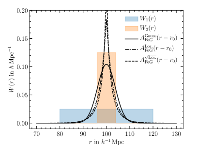
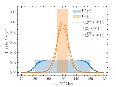
Figure 1: Left: Illustration of a wide top-hat window function $W_{1}(r)$ (blue shaded area), a narrow top-hat ($W_{2}(r)$, orange shaded area), and the three convolution kernels Eqs. 24–26 corresponding to the three models Eqs. 6–8. Right: The shaded areas are the same as in the left plot. If the window function in redshift space is a top-hat, then the real-space window function is a smoothed top-hat given by the convolution $A_{\mathrm{FoG}}*W\,(r)$, shown here for the same window functions and FoG models as in the left plot, see Eqs. 27–29.

The nonlinear RSD kernels $\widetilde{A}_{\rm nl}(\mu,k\mu)$ in Eqs. 6–8 only depend on $k\mu$, which yields one further simplication when computing the modified window function $\widetilde{A}_{\rm nl}(i\partial_{r^{\prime}})W_{r}(r^{\prime})$. Expressing the window function in terms of its Fourier transform $\widetilde{W}(q)$, we find that the modified window function is given as a convolution

$$\widetilde{A}_{\mathrm{nl}}(i\partial_{r^{\prime}})\,W_{r}(r^{\prime}) =\int_{-\infty}^{\infty}\frac{\mathrm{d}q}{2\pi}\,\widetilde{A}_{\mathrm{nl}}(-q)\,\widetilde{W}_{r}(q)\,e^{iqr^{\prime}}$$

$$=\int_{-\infty}^{\infty}\mathrm{d}y\,A_{\mathrm{nl}}(r^{\prime}-y)\,W_{r}(y)$$

$$\equiv A_{\mathrm{nl}}(r^{\prime})*W_{r}\,(r^{\prime})\,.$$ (23)

In deriving Eq. 23 we assumed that the domain of the window function, which is strictly speaking only defined for $r\geq 0$, can be extended to negative $r$ as well, and that it vanishes there.

Here, $A_{\mathrm{nl}}(r)$ is the inverse Fourier transform of $\widetilde{A}_{\mathrm{nl}}(q)$. Eq. 23 shows that the effective real-space window function is the radial convolution of the window function with the nonlinear RSD operator. The meaning of the RSD modification of the window function may be most apparent when applying the Fingers-of-God operators in Eqs. 6–8, for which the corresponding real-space functions are given by

$$A_{\mathrm{FoG}}^{\rm Gauss}(r^{\prime}-r) =\frac{1}{\sqrt{2\pi}\,\sigma_{u}}\,e^{-\frac{(r^{\prime}-r)^{2}}{2\sigma_{u}^{2}}}\,,$$ (24)

$$A_{\mathrm{FoG}}^{\rm Lor.}(r^{\prime}-r) =\frac{1}{\sqrt{2}\,\sigma_{u}}\,e^{-\frac{\sqrt{2}}{\sigma_{u}}\,|r^{\prime}-r|}\,,$$ (25)

$$A_{\mathrm{FoG}}^{\rm\sqrt{Lor.}}(r^{\prime}-r) =\frac{1}{\pi\sigma_{u}}\,K_{0}\!\left(\frac{|r^{\prime}-r|}{\sigma_{u}}\right)\,,$$ (26)

where $K_{n}(x)$ is a modified Bessel function of order $n$ (Taylor et al., 2001). Note that Eqs. 24–26 are simply the assumed 1D radial velocity distibution for each FoG model. The modified window function, therefore, incorporates the galaxies moving from the adjacent bins with the probability given by the velocity dispersion function (Kang et al., 2002; Percival et al., 2004; Loureiro et al., 2019).

For definiteness, we consider a case of radial binning with a top-hat window function of width $\Delta r_{i}$ centered on $r_{i}$: $W_{i}(r)=\frac{1}{\Delta r_{i}}$ when $r_{i}^{\mathrm{lo}}\leq r\leq r_{i}^{\mathrm{hi}}$ and vanishes otherwise, where $r_{i}^{\mathrm{lo}}=r_{i}-\frac{1}{2}\Delta r_{i}$ and $r_{i}^{\mathrm{hi}}=r_{i}+\frac{1}{2}\Delta r_{i}$ are the lower and upper bounds of the bin $i$. Then the modifed window functions given by the convolution in Eq. 23 are

$$A^{\rm Gauss}_{\mathrm{FoG}}*W_{i}\,(r) =\frac{\operatorname{erf}\!\left(\frac{r_{i}^{\mathrm{hi}}-r}{\sqrt{2}\,\sigma_{u}}\right)}{2\Delta r_{i}}-\frac{\operatorname{erf}\!\left(\frac{r_{i}^{\mathrm{lo}}-r}{\sqrt{2}\,\sigma_{u}}\right)}{2\Delta r_{i}}\,,$$ (27)

$$A^{\rm Lor.}_{\mathrm{FoG}}*W_{i}\,(r) =\frac{1}{2\Delta r_{i}}\,\frac{r_{i}^{\mathrm{hi}}-r}{|r_{i}^{\mathrm{hi}}-r|}\left(1-e^{-\frac{\sqrt{2}}{\sigma_{u}}|r_{i}^{\mathrm{hi}}-r|}\right)$$

$$\quad-\frac{1}{2\Delta r_{i}}\,\frac{r_{i}^{\mathrm{lo}}-r}{|r_{i}^{\mathrm{lo}}-r|}\left(1-e^{-\frac{\sqrt{2}}{\sigma_{u}}|r_{i}^{\mathrm{lo}}-r|}\right)\,,$$ (28)

$$A^{\rm\sqrt{Lor.}}_{\mathrm{FoG}}*W_{i}\,(r) =\frac{1}{\pi\,\Delta r_{i}}\int^{\frac{r_{i}^{\mathrm{hi}}-r}{\sigma_{u}}}_{\frac{r_{i}^{\mathrm{lo}}-r}{\sigma_{u}}}\mathrm{d}x\,K_{0}(|x|)\,,$$ (29)

where $\operatorname{erf}(x)\equiv\frac{2}{\sqrt{\pi}}\int_{0}^{x}\mathrm{d}t\,e^{-t^{2}}$ is the error function. The integration of the modified Bessel function in Eq. 29 can be expressed using the following identity:

$$\frac{1}{\pi}\int_{0}^{x}\mathrm{d}x^{\prime}\,K_{0}(x^{\prime}) =\frac{1}{2}\,x\,K_{0}\!\left(x\right)\,\mathbf{L}_{-1}\!\left(x\right)$$

$$\quad+\frac{1}{2}\,x\,K_{1}\!\left(x\right)\,\mathbf{L}_{0}\!\left(x\right)\,,$$ (30)

where ${\bf L}_{n}(x)$ is the modified Struve function of order $n$.

Should one use the phenomenological nonlinear RSD terms such as $\sum_{a,b}k^{a}\mu^{b}$ multiplied with the FoG factors, for example, as done in Shoji et al. (2009), one may need to calculate higher-order derivatives of the convolved window functions in Eqs. 27–29.

The left panel of Fig. 1 illustrates the convolution kernels Eqs. 24–26 for ($r_{0}=100\,~{}{\rm Mpc}/h$) and $\sigma_{u}=$3.8\text{\,}{\mathrm{\text{$h$}}}^{-1}\text{\,}\mathrm{Mpc}$$. For comparison we also show a wide top-hat bin of width $\Delta r=$40\text{\,}{\mathrm{\text{$h$}}}^{-1}\text{\,}\mathrm{Mpc}$$ (blue shaded box) and a narrow bin with $\Delta r=$8\text{\,}{\mathrm{\text{$h$}}}^{-1}\text{\,}\mathrm{Mpc}$$ (orange shaded box). We also show the modified window functions for the three FoG models and for the same two example top-hat functions in the right panel of Fig. 1.

The edges of the top-hat window function are smoothed by the convolution. This means that the galaxies contained in the top-hat bin $W(r)$ defined in the redshift-space are selected with a probability proportional to $A_{\mathrm{RSD}}*W\,(r)$ in real space. As expected, the modification of the window function (thus, the nonlinear RSD effect) is bigger for narrower window functions. For the narrow-window-function example ($\Delta r=8\,h^{-1}{\rm Mpc}$), about one third of the galaxies come from outside the top-hat boundaries. For the wide example ($\Delta r=40\,h^{-1}{\rm Mpc}$), only the edges are changed, so that only $\sim 8\text{\,}\mathrm{\char 37\relax}$ of galaxies are different between real space and redshift space. These effects are largest for Gaussian FoG, and smallest for square-root Lorentzian FoG.

IV Result: $C_{\ell}$ and $P(k_{\perp})$

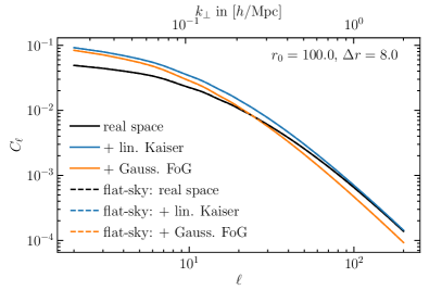
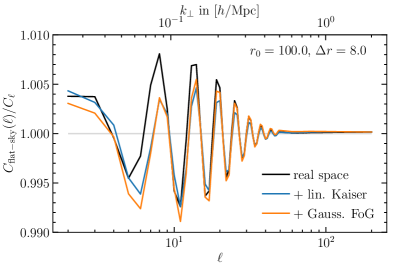
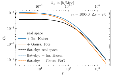
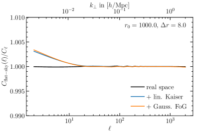
Figure 2: Comparison between the harmonic-space power spectra and the flat-sky approximation. The top two panels are for a top-hat window function of width $\Delta r=$8\text{\,}{\mathrm{\text{$h$}}}^{-1}\text{\,}\mathrm{Mpc}$$ centered around $r_{0}=$100\text{\,}{\mathrm{\text{$h$}}}^{-1}\text{\,}\mathrm{Mpc}$$, the bottom two panels are for $r_{0}=$1000\text{\,}{\mathrm{\text{$h$}}}^{-1}\text{\,}\mathrm{Mpc}$$ with the same width. Left panels: solid lines show the exact calculation, the dashed lines assume the flat-sky approximation. Right panels: the ratio between the flat-sky approximation and the exact calculation for the same narrow window function. To achieve below-percent-level agreement we use the correspondence Eq. 36. This same level of agreement is achieved with the Lorentzian and square-root-Lorentzian FoG models. All plots show the corresponding flat-sky $k_{\perp}$ mode on top.

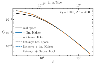
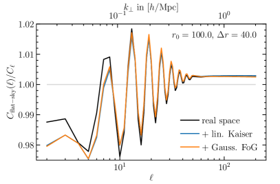
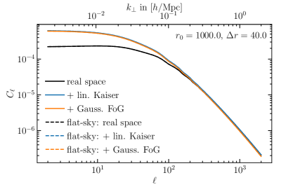
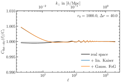
Figure 3: Same as Fig. 2 but with a bin width $\Delta r=$40\text{\,}{\mathrm{\text{$h$}}}^{-1}\text{\,}\mathrm{Mpc}$$.

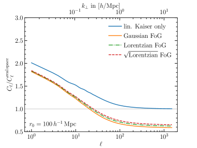
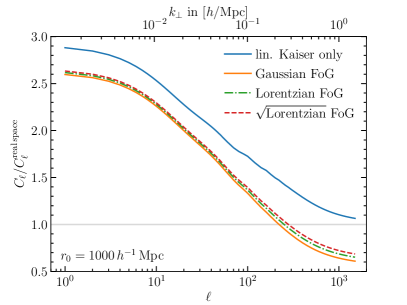
Figure 4: Ratio of RSD angular power spectra to the real-space angular power spectrum, for $r_{0}=$100\text{\,}{\mathrm{\text{$h$}}}^{-1}\text{\,}\mathrm{Mpc}$$ (left) and $r_{0}=$1000\text{\,}{\mathrm{\text{$h$}}}^{-1}\text{\,}\mathrm{Mpc}$$ (right). The bin width for both plots is $\Delta r=$8\text{\,}{\mathrm{\text{$h$}}}^{-1}\text{\,}\mathrm{Mpc}$$. For the three FoG models, the velocity dispersion is the same, and it is chosen according to Eq. 49. The limited width of the redshift bin introduces non-linearities such as the FoG on all transverse scales $\ell$. The corresponding transverse $k_{\perp}$-mode is shown at the top.

With the modified window functions shown in Fig. 1, we now compute the shape of the harmonic-space power spectrum with nonlinear redshift-space distortion. To apply the 2-FAST algorithm (Grasshorn Gebhardt and Jeong, 2018), we transform the integral over $r^{\prime}$ in Eq. 21 to an integral over the ratio $R=r^{\prime}/r$.

Along with the full harmonic space expression, we also compute the power spectrum with the flat-sky approximation. In the flat-sky calculation, we keep constant $\hat{z}$-direction throughout the volume, and compute the harmonic space powerspectrum by projecting the three-dimensional power spectrum along the parallel (line-of-sight) direction. The implementation of flat-sky approximation is easier as two of the three integrals in Eq. 21 can be done analytically. As we show in the following section, the flat-sky approximation provides a good approximation when matching $\ell=k_{\perp}r_{0}-\frac{1}{2}$ between the multipole moment and three-dimensional transverse Fourier wavenumber.

IV.1 Fourier-space expression with the flat-sky approximation

With the flat-sky approximation, we obtain the tangential two-dimensional (${\bm{x}}_{\perp}$) density contrast by integrating the three-dimensional density contrast along the line-of-sight,

$$\delta_{s}({\bm{x}}_{\perp}) =\int\mathrm{d}z\,W(z)\,\delta_{s}({\bm{x}})\,,$$ (31)

where $\delta_{s}({\bm{x}})$ is the redshift space density contrast, and $W(z)$ is the radial window function. The Fourier-space density contrast is then,

$$\delta_{s}({\bm{k}}_{\perp}) =\int\mathrm{d}^{2}x_{\perp}\,\delta_{s}({\bm{x}}_{\perp})\,e^{-i{\bm{k}}_{\perp}\cdot{\bm{x}}_{\perp}}\,.$$ (32)

Expressing the density contrast $\delta_{s}({\bm{x}})$ in terms of its Fourier components $\delta_{s}({\bm{k}})$ allows us to perform the integrals over ${{\bm{x}}}_{\perp}$ analytically. We get

$$\delta_{s}({\bm{k}}_{\perp}) =\int\mathrm{d}^{2}x_{\perp}\left[\int dz\,W(z)\int\frac{d^{3}q}{(2\pi)^{3}}\,\delta_{s}({\bm{q}})\,e^{i{\bm{q}}\cdot{\bm{x}}}\right]e^{-i{\bm{k}}_{\perp}\cdot{\bm{x}}_{\perp}}$$

$$=\int\frac{\mathrm{d}k_{z}}{2\pi}\,\delta({\bm{k}})\,\widetilde{A}_{\mathrm{RSD}}\left(\frac{k_{z}}{k},k_{z}\right)\,\widetilde{W}^{*}(k_{z})\,,$$ (33)

where we used Eq. 4, $\mu\equiv{\hat{\bm{z}}}\cdot{\hat{\bm{k}}}$, and $\widetilde{W}(k_{z})$ is the Fourier transform of the window function. Defining the perpendicular two-dimensional power spectrum as

$$\left\langle\delta_{s}({\bm{k}}_{\perp})\delta_{s}^{*}({\bm{k}}^{\prime}_{\perp})\right\rangle =(2\pi)^{2}\delta^{D}({\bm{k}}_{\perp}-{\bm{k}}^{\prime}_{\perp})\,C(k_{\perp})\,,$$ (34)

we find that

$$C(k_{\perp};r_{1},r_{2}) =\int\frac{\mathrm{d}k_{z}}{2\pi}\,P(k)\,\widetilde{W}^{*}_{1}(k_{z})\,\widetilde{W}_{2}(k_{z})$$

$$\quad\times\widetilde{A}_{\mathrm{RSD}}^{r_{1}}\!\left(\frac{k_{z}}{k},k_{z}\right)\,\widetilde{A}_{\mathrm{RSD}}^{r_{2}*}\!\left(\frac{k_{z}}{k},k_{z}\right)\,,$$ (35)

with $k=\sqrt{k_{\perp}^{2}+k_{z}^{2}}$, and the superscript $r_{i}$ in $\widetilde{A}_{\mathrm{RSD}}$ indicates the radial-dependence of the coefficients, for example $f(r_{i})$ and $\sigma_{u}(r_{i})$, of $\widetilde{A}_{\rm RSD}$. Note that, in Eq. 35 we assume that the power spectrum $P(k)$ does not depend on redshift, but we can easily include the time-dependence into the $\widetilde{A}_{\rm RSD}$. For example, the linear growth factor $D(r_{1})D(r_{2})$ would introduce a constant multiplication factor to $\widetilde{A}_{\rm RSD}$.

In order to relate Eq. 35 to the angular power spectrum, we convert the two-dimensional Fourier wavenumber $k_{\perp}$ to the harmonic space moment $\ell$ as, $\ell+\frac{1}{2}=k_{\perp}r_{0}$, (Grasshorn Gebhardt and Jeong, 2018) , where $r_{0}\equiv\frac{1}{2}(r_{1}+r_{2})$, and

$$C_{\ell} =\frac{1}{r_{1}r_{2}}\,C\left(k_{\perp}=\frac{\ell+1/2}{r_{0}}\right)\,.$$ (36)

For a top-hat window function of width $\Delta r_{i}$ centered around $r_{i}$, we have $W_{i}(z)=1/\Delta r_{i}$, and the Fourier transform is

$$\widetilde{W}_{i}(k_{z}) =\,e^{-ik_{z}r_{i}}\,j_{0}\!\left(\frac{k_{z}\Delta r_{i}}{2}\right)\,,$$ (37)

where $j_{0}(x)\equiv\sin(x)/x$ is the spherical Bessel function of order 0. Therefore, the cross-correlation between two bins of widths $\Delta r_{1}$ and $\Delta r_{2}$ centered on $r_{1}$ and $r_{2}$ is in the flat-sky approximation given by

$$C(k_{\perp},r_{1},r_{2}) =\int\frac{\mathrm{d}k_{z}}{2\pi}\,P(k)\,\cos\!\left(k_{z}(r_{1}-r_{2})\right)$$

$$\quad\times j_{0}\!\left(\frac{k_{z}\Delta r_{1}}{2}\right)\,j_{0}\!\left(\frac{k_{z}\Delta r_{2}}{2}\right)$$

$$\quad\times\widetilde{A}_{\mathrm{RSD}}^{r_{1}}\!\left(\frac{k_{z}}{k},k_{z}\right)\widetilde{A}_{\mathrm{RSD}}^{r_{2}*}\!\left(\frac{k_{z}}{k},k_{z}\right)\,,$$ (38)

where the imaginary part vanishes since all terms other than the exponential are even in $k_{z}$, and we assume that the RSD factor is real, e.g., as in Eqs. 5, 6, 7 and 8. Using Eq. 38, we find the auto-correlation function as

$$C(k_{\perp},r_{0}) =\int\frac{\mathrm{d}k_{z}}{2\pi}\,P(k)\left[j_{0}\!\left(\frac{k_{z}\Delta r}{2}\right)\widetilde{A}_{\mathrm{RSD}}^{r_{0}}\!\left(\frac{k_{z}}{k},k_{z}\right)\right]^{2}\,,$$ (39)

where we set $r_{0}=r_{1}=r_{2}$ and $\Delta r=\Delta r_{1}=\Delta r_{2}$.

IV.2 Small-scale ($k_{\perp}\to\infty$ or $\ell\to\infty$) limit

In the small-tangential (angular) scale limit where $k_{\perp}\to\infty$, we get for the auto-correlation

$$\lim_{k_{\perp}\to\infty}C(k_{\perp}) =P(k_{\perp})\int\frac{\mathrm{d}k_{z}}{2\pi}\,\left|\widetilde{A}_{\mathrm{RSD}}\!\left(0,k_{z}\right)\,\widetilde{W}(k_{z})\right|^{2}\,.$$ (40)

That is, the suppression of the power spectrum due to FoG becomes independent of $k_{\perp}$, or $\ell$. As the flat-sky approximation is valid on small scales, we expect that the same is true for the exact calculation as well. The suppression factor for a top-hat window function and Gaussian FoG relative to real space only depends on the width of the window function $\Delta r$ and the velocify dispersion $\sigma_{u}$:

$$\frac{\int\frac{\mathrm{d}k_{z}}{2\pi}\,\left|\widetilde{A}_{\mathrm{RSD}}\!\left(0,k_{z}\right)\,\widetilde{W}(k_{z})\right|^{2}}{\int\frac{\mathrm{d}k_{z}}{2\pi}\,\left|\widetilde{W}(k_{z})\right|^{2}}$$

$$=\operatorname{erf}\!\left(\frac{\Delta r}{2\sigma_{u}}\right)-\frac{2\sigma_{u}}{\sqrt{\pi}\,\Delta r}\left(1-e^{-\frac{\Delta r^{2}}{4\sigma_{u}^{2}}}\right)\,.$$ (41)

Similar expressions can be found for other forms of the FoG.

IV.3 Nonlinear RSD in Harmonic space $C_{\ell}$

In Fig. 2 we show the harmonic-space power spectra calculation for a window function of width $\Delta r=$8\text{\,}{\mathrm{\text{$h$}}}^{-1}\text{\,}\mathrm{Mpc}$$ centered around $r_{0}=$100\text{\,}{\mathrm{\text{$h$}}}^{-1}\text{\,}\mathrm{Mpc}$$ (top panels) and we repeat this for a window function of the same width centered around $r_{0}=$1000\text{\,}{\mathrm{\text{$h$}}}^{-1}\text{\,}\mathrm{Mpc}$$ (bottom panels). For each case, we show the real-space power spectrum, the RSD power spectrum with only the linear Kaiser effect (without $\widetilde{A}_{\rm nl}$ in Eq. 5), and the power spectrum that includes the linear Kaiser effect and Gaussian FoG.

In Fig. 2, we notice a few RSD features in harmonic space with narrow radial binning. First, as we expect from the three-dimensional RSD, the linear Kaiser effect enhances the power spectrum on large scales. The linear Kaiser effect, however, in harmonic space shows a strong scale-dependence, and the enhancement vanishes on small scales. Second, unlike the three-dimensional RSD, the Fingers-of-God effect reduces the power spectrum on all scales, but more so on small scales. This is because the modified window function affects the angular clustering on all scales.

In addition, Fig. 2 shows that the flat-sky approximation (dashed line) agrees quite well with the exact result in harmonic space (solid line) on all scales. As shown in the right panels of Fig. 2, Eq. 39 leads to an agreement between the full formula and the flat-sky formula better than $0.8\text{\,}\mathrm{\char 37\relax}$ for the narrow window function considered here. The bottom panel shows that the flat-sky approximation proves to be more accurate at the larger radius $r_{0}=$1000\text{\,}{\mathrm{\text{$h$}}}^{-1}\text{\,}\mathrm{Mpc}$$. With a wider window function $\Delta r=$40\text{\,}{\mathrm{\text{$h$}}}^{-1}\text{\,}\mathrm{Mpc}$$ as shown in Fig. 3 the differences become larger. We also find that the agreements between the exact and flat-sky calculations holds the same for the Lorentzian and square-root-Lorentzian FoG cases. Note the sub-percent deviation at high $\ell$ for the $\Delta r=40\,h^{-1}{\rm Mpc}$ case shown in the top-right panel of Fig. 3. As the analysis in Section IV.4 below shows, the discrepancy comes from the large $\Delta r/r$ for which the flat-sky approximation breaks. Nevertheless, the difference stays quite small even for this rather pathological example with $r=100\,h^{-1}{\rm Mpc}$ and $\Delta r=40\,h^{-1}{\rm Mpc}$.

Given the excellent agreement between the exact calculation and the flat-sky approximation, we can understand the FoG effect on large angular scales as follows. In the $k_{\perp}\to 0$ limit, the flat-sky formula gives (for Gaussian FoG as an example here)

$$C(0,r_{0}) =(1+\beta)^{2}\int\frac{\mathrm{d}k_{z}}{2\pi}\,P(k_{z})\,j_{0}^{2}\!\left(\frac{k_{z}\Delta r}{2}\right)e^{-\sigma_{u}^{2}k_{z}^{2}}$$ (42)

The spherical Bessel ensures that all modes up to $k_{z}\lesssim\frac{\pi}{\Delta r}$ contribute, while the FoG suppression factor, on the other hand, affects scales $k_{z}\gtrsim 1/\sigma_{u}$. The large-angular scale power spectrum is affected by the FoG effect if $1/\sigma_{u}\lesssim\pi/\Delta r$, or $\Delta r\lesssim\pi\sigma_{u}$. For example, when $\sigma_{u}\sim 3{\rm Mpc}/h$, the large angular-scale power spectrum for $\Delta r=8\,{\rm Mpc}/h<\pi\sigma_{u}=10{\rm Mpc}/h$ must be affected by FoG, but not for $\Delta r=40\,{\rm Mpc}/h>\pi\sigma_{u}=10{\rm Mpc}/h$. That is consistent with what we observe in Figs. 2–3.

In Fig. 4, we compare the three forms for the FoG by showing the ratio of the RSD angular power spectrum to the real-space angular power spectrum in each case. Additionally, the figure shows the ratio for the Kaiser effect only, and in the left panel we use $r_{0}=$100\text{\,}{\mathrm{\text{$h$}}}^{-1}\text{\,}\mathrm{Mpc}$$ and in the right panel $r_{0}=$1000\text{\,}{\mathrm{\text{$h$}}}^{-1}\text{\,}\mathrm{Mpc}$$.

Again, Fig. 4 shows that the Kaiser effect vanishes on small scales, and the FoG, while present on all scales, is strongest on small scales. Furthermore, the three forms of the FoG are very similar. As may be expected from Fig. 1, Gaussian FoG are strongest while a square-root Lorentzian is weakest for the same $\sigma_{u}$. The functional form is also different in that a Gaussian FoG has a larger difference between large and small scales than the other two. We have checked that this also holds true even if $\sigma_{u}$ is adjusted so that the three forms agree on small scales using the analytical formula in Section IV.2.

IV.4 Limber’s approximation

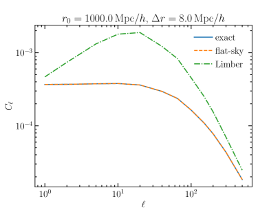
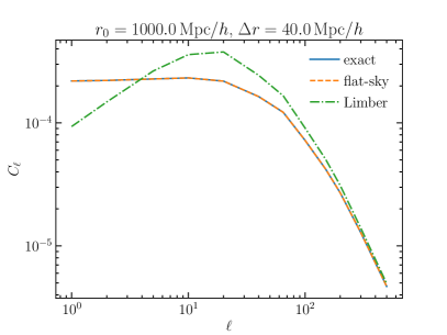
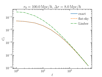
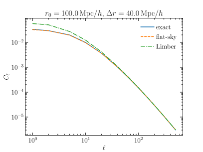
Figure 5: The real-space $C_{\ell}$ calculated using three different formulas: In blue the exact formula, in orange the flat-sky (almost directly on top of the blue line), in green Limber’s approximation. Limber’s approximation works better when the bin width is large. The corresponding $k_{\perp}$-mode is obtained by $k_{\perp}=(\ell-\frac{1}{2})/r_{0}$.

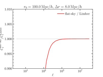
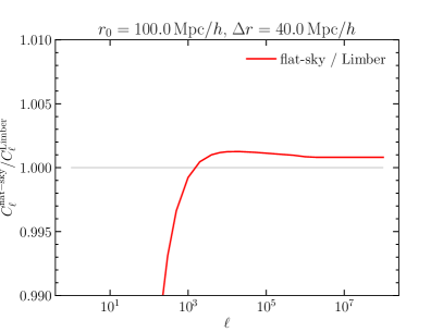
Figure 6: Ratio of flat-sky to Limber in real space. Only at very high $\ell$ is the predicted difference between flat-sky and Limber Eq. 46 reached. This figure assumes that the power spectrum remains a power-law far into the non-linear regime.

The top-right panel of Fig. 3 shows a constant discrepancy between the full calculation and the flat-sky approximation. In this section, we study the origin of this difference by comparing the flat-sky approximation and the Limber approximation which provides an accurate approximation for large $\ell$.

Limber’s approximation may be written as (Loverde and Afshordi, 2008)

$$j_{\ell}(kr)\to\sqrt{\frac{\pi}{2kr}}\,\delta^{D}\!\left(kr-\ell-\frac{1}{2}\right)\,.$$ (43)

Then, Eq. 21 in real space for an auto-correlation can be approximated as

$$C_{\ell}^{\mathrm{Real\,space}} =\int\mathrm{d}r\,\frac{W^{2}\!\left(r\right)}{r^{2}}\,P_{g}\!\left(\frac{\ell+\frac{1}{2}}{r}\right),$$ (44)

and narrow window functions will enforce that $k\simeq\frac{1}{r_{0}}(\ell+\frac{1}{2})$, where $r_{0}$ is the radius to the bin center. For a power-law power spectrum $P(k)\propto k^{-(3+\epsilon)}$ and top-hat window we then get, to first order:

$$C_{\ell}^{\mathrm{Real\,space}} =\frac{1}{r_{0}^{2}\Delta r}\,P_{g}\!\left(\frac{\ell+\frac{1}{2}}{r_{0}}\right)\left(1+\epsilon\frac{\Delta r^{2}}{8r_{0}^{2}}\right)$$ (45)

$$=\frac{C\!\left(k_{\perp}\right)}{r_{0}^{2}}\left(1+\epsilon\,\frac{\Delta r^{2}}{8r_{0}^{2}}\right)\,,$$ (46)

with the flat-sky approximation $C(k_{\perp})$. Here, we assume that both $\Delta r/r$ and $|\epsilon|$ are small so that $\ln(r+\Delta r/2)\simeq\ln(r)+\frac{\Delta r}{2r}$ and $r_{0}^{\epsilon}\simeq 1+\epsilon\ln(r_{0})$. The last equality follows from the flat-sky Eq. 40 when $A_{\mathrm{RSD}}=1$ and the window is a top-hat.

Eq. 46 clearly shows that the flat-sky approximation has an intrinsic inaccuracy on small scales that is proportional to the relative bin width $\Delta r^{2}/r^{2}$, and depends on the slope of the power spectrum $-(3+\epsilon)$. This is the source of the discrepancy on small scales between the exact calculation and the flat-sky calculation in the top-right panel of Fig. 3. This is somewhat complimentary to Limber’s approximation which works better for larger radial bins Jeong et al. (2009).

Physically, the flat-sky discrepancy on small scales comes from treating transverse separations for a given angle the same, whether they are at the far end or the near end of the redshift bin. However, the ratio of these transverse separations is $(r_{0}+\frac{1}{2}\Delta r)/(r_{0}-\frac{1}{2}\Delta r)\approx 1+\Delta r/r_{0}$ for small angles. Hence, the ratio $\Delta r/r_{0}$ appears in Eq. 46. The shape of the power spectrum also clearly matters, as evaluating the power spectrum at smaller than center-of-bin scales at the near end and larger-than-center-of-bin scales at the far end cancel only when $P(k)\propto k^{-3}$. We, however, stress here that the difference stays sub-percent level even for the pathological case ($\Delta r/r_{0}=0.4$) shown here.

The real-space comparison in Fig. 5 among the full calculation (blue solid lines), flat-sky approximation (orange dashed lines), and Limber approximation (Green dot-dashed lines) clearly shows that the flat-sky approximation outperforms the Limber approximation. While the flat-sky and exact calculations lie virtually on top of each other with percent-level discrepancies (also see Figs. 2 and 3), Limber’s approximation does not approach the exact calculation until very large $\ell$.

Incidentally, this large $\ell$ is also when the flat-sky approximation starts to break down. Fig. 6 compares the flat-sky and Limber’s approximation up until such high $\ell$ that the ratio becomes constant, and is in rough agreement with Eq. 46 as well as the discrepancy shown in the top-right panel of Fig. 3.

V RSD in Log-normal simulation

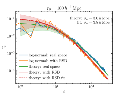
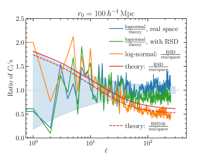
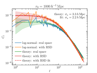
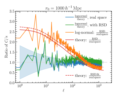
Figure 7: Comparison between theoretical calculation and log-normal simulations for a top-hat window function of width $\Delta r=$8\text{\,}{\mathrm{\text{$h$}}}^{-1}\text{\,}\mathrm{Mpc}$$, at $r_{0}=$100\text{\,}{\mathrm{\text{$h$}}}^{-1}\text{\,}\mathrm{Mpc}$$ (top) and $r_{0}=$1000\text{\,}{\mathrm{\text{$h$}}}^{-1}\text{\,}\mathrm{Mpc}$$ (bottom). The left plots show the angular power spectrum with and without RSD, the left plots show the ratios between angular power spectra as indicated in the legend. For the solid theory lines we used Eq. 49 to calculate $\sigma_{u}$, for the dashed line we chose a value that leads to better match to the simulation result. The corresponding $k_{\perp}$-mode is obtained by $k_{\perp}=(\ell-\frac{1}{2})/r_{0}$.

Finally, in this section we compare the harmonic-space nonlinear RSD expression Eq. 21 with the result from a log-normal simulation (Agrawal et al., 2017). Again, we adopt a top-hat window function of width $\Delta r=$8\text{\,}{\mathrm{\text{$h$}}}^{-1}\text{\,}\mathrm{Mpc}$$, and consider two radii of $r_{0}=$100\text{\,}{\mathrm{\text{$h$}}}^{-1}\text{\,}\mathrm{Mpc}$$ and $r_{0}=$1000\text{\,}{\mathrm{\text{$h$}}}^{-1}\text{\,}\mathrm{Mpc}$$.

For the $r_{0}=$100\text{\,}{\mathrm{\text{$h$}}}^{-1}\text{\,}\mathrm{Mpc}$$ simulation, we generate a cubic box with length $L_{x}=L_{y}=L_{z}=300$ and grid size $N=600$ so that the resolution is $0.5\text{\,}{\mathrm{\text{$h$}}}^{-1}\text{\,}\mathrm{Mpc}$. We draw $\sim 2\text{\times}{10}^{6}$ galaxies. We then position the observer at the center of this box, we shift the galaxies according to their line-of-sight velocity using

$$s =r+\frac{{\bm{v}}\cdot{\hat{\bm{r}}}}{aH}\,,$$ (47)

where ${\hat{\bm{r}}}$ is the line-of-sight unit vector. We then apply a top-hat radial window function by limiting the sample to galaxies with redshift-space distances $r_{0}-\frac{1}{2}\Delta r\leq r\leq r_{0}+\frac{1}{2}\Delta r$, where $\Delta r=$8\text{\,}{\mathrm{\text{$h$}}}^{-1}\text{\,}\mathrm{Mpc}$$ and $r_{0}=$100\text{\,}{\mathrm{\text{$h$}}}^{-1}\text{\,}\mathrm{Mpc}$$. This results in a sample of $N_{\mathrm{gal}}=$7.7\text{\times}{10}^{5}$$ galaxies in a spherical shell around the observer. The angular power spectrum is measured from the simulation using the healpy software with $N_{\mathrm{side}}=1024$ and distributing galaxies to their nearest grid point on the sky. To measure the real-space angular power spectrum, we repeat this without shifting the galaxies according to Eq. 47.

For the second simulation we repeat this procedure with a cube of side length $L=$2160\text{\,}{\mathrm{\text{$h$}}}^{-1}\text{\,}\mathrm{Mpc}$$, grid size $N=2160$, $n_{\mathrm{side}}=2048$, and a total of ${10}^{9}$ galaxies. We then draw galaxies around $r_{0}=$1000\text{\,}{\mathrm{\text{$h$}}}^{-1}\text{\,}\mathrm{Mpc}$$, leading to a sample of $N_{\mathrm{gal}}=$9.9\text{\times}{10}^{6}$$ galaxies in a shell around the observer.

We estimate the measurement uncertainty by

$$\Delta C_{\ell} =\sqrt{\frac{2}{2\ell+1}}\left(C_{\ell}+\frac{4\pi}{N_{\mathrm{gal}}}\right)\,,$$ (48)

but for the examples that we show here, the shot-noise contribution is negligibly small: that is what we have intended in order to test the RSD predictions on smaller scales.

In Fig. 7, we show the harmonic-space nonlinear RSD power spectrum from the log-normal simulations at low redshift ($r_{0}=100$ top panel) and high redshift ($r_{0}=1000$ bottom panel), along with corresponding theoretical predictions from Eq. 21. For both cases, the left panels show the power spectra for two cases (1) without RSD (real space), and (2) with RSD (Kaiser effect + Gaussian FoG model). To facilitate the comparison, we show various ratios of the angular power spectrum in the right panels: the ratio of the log-normal simulation to the theoretical calculation both in real space and in redshift space, and the ratio of redshift space to real space for both the log-normal simulation and theoretical calculation. For all cases, we find an excellent agreement between the simulation result and the result from Eq. 21.

For the solid lines in Fig. 7, we use the FoG model with the theoretical prediction for the one-dimensional velocity dispersion:

$$\sigma_{u}^{2}=\left\langle s^{2}\right\rangle-\left\langle s\right\rangle^{2}=\frac{\left\langle({\bm{v}}\cdot{\hat{\bm{r}}})^{2}\right\rangle}{a^{2}H^{2}} =\frac{f^{2}}{3}\int\frac{\mathrm{d}^{3}k}{(2\pi)^{3}}\,\frac{P_{m}(k)}{k^{2}}\,,$$ (49)

where $P_{m}(k)$ is the matter power spectrum used as input to the simulations. This results in the values indicated by “theory” in the top-right corners of the panels on the left. We, however, find that we can achieve a better match by fitting the velocity dispersion $\sigma_{u}$. The values we chose are labeled “fit” in the figure, and the fitting results are shown as the dashed lines.

VI Conclusion

In this paper, we present a novel method of calculating the harmonic-space galaxy power spectrum including the nonlinear Kaiser effect. The general formula in Eq. 21 states that nonlinear Kaiser effect can be modeled by modifying the radial window function.

We then apply the formula to model the nonlinear Fingers of God effect (FoG). We show that the FoG is equivalent to a smoothing of the radial window function, and, unlike the three-dimensional RSD effect in Fourier space, the FoG changes the harmonic-space power specturm on all scales. We considered Gaussian, Lorentzian, and square-root-Lorentzian forms [Eqs. 6–8] for the FoG. We show that for narrow window functions the flat-sky approximation agrees with the wide-angle analysis within a few tenths of a percent on all scales $\ell\geq 2$ if we make the identification $k_{\perp}r_{0}=\ell+0.5$. We also show that the flat-sky approximation has a residual inaccuracy proportional to $(\Delta r/r)^{2}$ on all scales. The flat-sky approximation, therefore, is most suitable for narrow radial bins, and is complementary to Limber’s approximation which is suitable for broader radial bins.

Comparing with the log-normal simulations shows an excellent agreement, provided that the velocity dispersion parameter $\sigma_{u}^{2}$ is chosen to fit the resulting power spectrum. The best-fitting $\sigma_{u}^{2}$ differs from the measured variance in the line-of-sight pairwise velocity distribution function.

Note that the present paper only considers the auto-correlation with a thin redshift bin. As the flat-sky approximation has indicated, we are, therefore, primarily probing the clustering on the tangential directions, and we lost radial correlation among different radial bins. To fully exploit the three-dimensional galaxy distribution, it is therefore necessary to consider cross-correlations as well. Eq. 21 can also be used for such a task, and we leave the details for a future investigation.