Kernelized Stein Discrepancy Tests of Goodness-of-fit for Time-to-Event Data††thanks: TF, WX, AG are grateful for the support from the Gatsby Charitable Foundation. NR is supported by Thomas Sauer- wald’s ERC Starting Grant 679660.
Abstract
Survival Analysis and Reliability Theory are concerned with the analysis of time-to-event data, in which observations correspond to waiting times until an event of interest such as death from a particular disease or failure of a component in a mechanical system. This type of data is unique due to the presence of censoring, a type of missing data that occurs when we do not observe the actual time of the event of interest but, instead, we have access to an approximation for it given by random interval in which the observation is known to belong. Most traditional methods are not designed to deal with censoring, and thus we need to adapt them to censored time-to-event data. In this paper, we focus on non-parametric goodness-of-fit testing procedures based on combining the Stein’s method and kernelized discrepancies. While for uncensored data, there is a natural way of implementing a kernelized Stein discrepancy test, for censored data there are several options, each of them with different advantages and disadvantages. In this paper, we propose a collection of kernelized Stein discrepancy tests for time-to-event data, and we study each of them theoretically and empirically; our experimental results show that our proposed methods perform better than existing tests, including previous tests based on a kernelized maximum mean discrepancy.
1 Introduction
An important topic of study in statistics is the distribution of times to a critical event, otherwise known as survival times: examples include the infection time from a disease Andersen et al., [2012]; Mirabello et al., [2009]; the death time of a patient in a clinical trial Collett, [2015]; Biswas et al., [2007]; or the possible re-offending times for released criminals Chung et al., [1991]. Survival data are frequently subject to censoring: the time of interest is not observed, but rather a bound on it. The most common scenario studied is right censoring, where a lower bound on the survival time is observed, for instance, a patient might leave a clinical trial before it is completed, meaning that we only obtain a lower bound on the time of death (the definitions and terminologies for the survival analysis setting will be provided in Section 2).
We address the setting where a model of survival times is proposed, and it is desired to test this model against observed data in the presence of censoring: this is known as goodness-of-fit testing. When departures from the model follow a known parametric family, a number of classical tests are available, being the most popular in practice the Log-rank test Hollander and Proschan, [1979], and its generalization, the weighted Log-rank test Brendel et al., [2014]. For an overview of these and other methods we refer the reader to Klein and Moeschberger, [2006]
In the event of more general departures from the null, kernel methods may be used to construct a powerful class of non-parametric tests to detect a greater range of alternative scenarios. For the uncensored case, a popular class of kernel goodness-of-fit tests utilize Stein’s method Barbour and Chen, [2005]; Chen et al., [2010]; Ley et al., [2017]; Gorham and Mackey, [2015] to develop a test statistic Liu et al., [2016]; Chwialkowski et al., [2016]; Gorham and Mackey, [2017]; Jitkrittum et al., [2017], which can be computed even when the model is known only up to normalization. In this paper we consider the particular case of kernel Stein discrepancies (KSDs) which are described in Section 2. While an alternative strategy would be simply to run a two-sample test using samples from the model, using for instance the maximum mean discrepancy (MMD) Gretton et al., [2012], Stein tests are more computationally efficient (no additional sampling is needed), and can take advantage of model structure to achieve better test power. KSD tests have been extended to various settings such as discrete variable models Yang et al., [2018], point process Yang et al., [2019], latent variable models Kanagawa et al., [2019], and directional data Xu and Matsuda, [2020].
In the present work, we propose to generalize Stein goodness-of-fit tests to the setting of survival analysis with right-censored data. In Section 3, we introduce three separate approaches to constructing a Stein operator in the presence of censoring: the first, the Survival Stein Operator, is the most direct generalization of the Stein operator used in the uncensored KSD test. The second, the Martingale Stein Operator, uses a different construction, based on a classical martingale studied in the survival analysis literature. The third, the Proportional Stein Operator, is designed for composite null hypotheses: in this case, the hazard function (that is, the instantaneous probability of an event at a given time, conditioned on survival to that time) is known only up to a constant of proportionality. For instance, we may wish to use a constant hazard as the null hypothesis, without specifying in advance the value of the constant.
The rest of the paper is structured as follows: in Section 4, we construct kernel statistics of goodness-of-fit, based on each of the operators previously introduced. We characterize the asymptotics of each statistic in Section 5. We find that in order to guarantee convergence in distribution under the null, the kernel statistic based on the Survival Stein Operator requires more restrictive conditions than the statistic built on the Martingale Stein Operator. In other words, the straightforward extension of the uncensored test is in fact the more restrictive approach of the two. Stronger assumptions again are required in obtaining convergence in distribution for the Proportional Stein Operator statistic, which should come as no surprise, given that the null is now an entire model class. For each statistic, we propose a wild bootstrap approach to obtain the test threshold. Empirical studies and results are presented in Section 6, where we compare with a recent state-of-the-art non-parametric test for censored data by Fernandez and Gretton, [2019] based on the MMD, which has been shown to outperform classical tests. For challenging cases, our Stein tests surpass the MMD test.
2 Background
Kernel Stein Discrepancy
We briefly review the kernel Stein discrepancy (KSD) in the absence of censoring Chwialkowski et al., [2016]; Liu et al., [2016], which is inspired from Gorham and Mackey, [2015]; Ley et al., [2017]. Let be a smooth probability density on . For a bounded smooth function , the Stein operator is given by
| (2.1) |
where ′ denotes derivative w.r.t . Since vanishes at the boundary and is bounded, integration by parts on results in Stein’s Lemma:
under some regularity conditions. Since the Stein operator depends on the density only through the derivative of , it does not involve the normalization constant of , which is a useful property for dealing with unnormalized models Hyvärinen, [2005].
Let be a reproducing kernel Hilbert space (RKHS) on with associated kernel . By using the Stein operator above, the kernel Stein discrepancy (KSD) Chwialkowski et al., [2016]; Liu et al., [2016] between two densities and is defined as
| (2.2) |
where denotes the unit ball of , and denotes the expectation w.r.t. the density . It is easy to see that and that for . Moreover, under some regularity conditions, we have that if and only if Chwialkowski et al., [2016].
By using standard properties of RKHSs, we can conveniently write as
| (2.3) |
where
with denoting the inner product of .
Censored Data
Let be the survival times, which are non-negative real-valued random variables of interest, and let be another collection of non-negative random variables called censoring times. In this work, we assume the non-informative censoring setting, where the censoring times are independent of the survival times. The data we observe correspond to where and . We can imagine that is the time of interest (death of a patient) and is the time a patient leaves the study for some other reason, thus, for some patients we observe their actual death time, whereas for others we just observe a lower bound (the time they left the study). indicates if we are observing or .
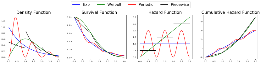
We denote by , and , the respective density functions associated with the random variables , and . Similarly, we denote by , and , the respective cumulative distribution functions; and by , and , the survival functions. An important element in survival analysis is the hazard function which represents the instantaneous risk of dying at a given time (as usually refers to a death time). Given a distribution with density and survival function , the hazard function is given by , which can be seen as the density at of a random variable conditioned on the event . The corresponding cumulative hazard function is defined as . A useful feature of the hazard function is that there is a one-to-one relation between hazard and density functions through the relation . For the random variables and , we denote by and their respective hazard functions, and by and , their cumulative hazards functions. As a remark, every continuous non-negative function can be a hazard function, as long as , thus, describing hazards is much easier than describing densities, as we do not need to worry about normalization constants. Examples of corresponding functions for different models are displayed in Figure 1.
As observations correspond to pairs , it is convenient to consider the joint measure on induced by the pair . We write to denote the measure when the survival times of interest are generated according to , and if they are generated under (i.e., under the null). Note that and also depend on , however we don’t make this dependence explicit, since for goodness-of-fit we only care about and .
Finally, for any function , the following identities hold, which the reader should keep in mind for later use:
| (2.4) | ||||
| (2.5) |
Here means that we are taking expectation w.r.t. . Similarly, we write to indicate (under the null hypothesis).
3 Stein Operator for Censored Data
In this section, we describe a set of Stein operators for censored data. We denote by the set of functions , and recall that is the measure induced by data under the null hypothesis.
Definition 1.
Let . We call a Stein operator for if for each
| (3.1) |
An interesting technical point is that our operator takes functions and maps them to . The idea behind having these two spaces is that while our data of interest is a time (hence the space of functions ), we actually observe pairs , hence we need functions in .
We choose the general class to be an RKHS. We assume that contains only differentiable and bounded functions, and that if then . These requirements are not restrictive and most of the standard kernels in the literature generate RKHSs with these properties, including the Gaussian kernel (furthermore, we can avoid this restriction, but we keep it as it is convenient for the exposition of the paper). Further properties of will be imposed if needed in particular cases.
3.1 Survival Stein Operator
Observe that if and only if . One might be tempted to use only the uncensored observations to approximate (where is the standard Stein operator in (2.1)) by computing
however, this sum does not converge to as the term introduces bias due to censoring. Indeed, such an empirical average converges to . To account for this bias we redefine as
| (3.2) |
Here we write instead of whenever we assume that the additional condition is satisfied,
| (3.3) |
which guarantees that the operator is well-defined. Notice that in equation (3.2) appears since we do not necessarily assume a vanishing boundary at 0.
Under the null hypothesis, , it holds that
| (3.4) |
as the number of data points tends to infinity, and due to Equation (2.4) and the fact that
| (3.5) |
which is proved using integration by parts. Notice that in this argument we use that only contains bounded functions, allowing us to get rid of the boundary at infinity.
The operator can be seen as a natural extension of the Stein operator Gorham and Mackey, [2015] to censored data. Observe that in the uncensored case, recovers the standard Stein operator.
Unfortunately, in the goodness-of-fit setting, we only have access to the null distribution but not to the censoring distribution , thus needs to be estimated. The standard estimator for is the Kaplan-Meier estimator Kaplan and Meier, [1958] which is very data inefficient, leading to an unsatisfactory testing procedure.
To bypass the approximation of we define the survival Stein operator as
| (3.6) |
The previous proposition says that if the data we observed was generated from then the expectation of the operators and are equal for each function in . However, the relation between and is stronger than merely equality in expectation, indeed, under a slightly stronger condition on the form of the distribution and we get the following result, which is proven in Appendix A.
Proposition 3.
Assume that
| (3.7) |
then, under the null hypothesis, i.e. , we have that, as the number of data points tends to infinity,
To better understand the survival Stein operator, we interpret the proposed Stein operator by making connections to the Stein operator used in the uncensored case.
A careful computation gives the following equivalent expression for the expectation of for :
Here, we can relate the first expectation to uncensored observations: ; the second expectation to censored observations: ; and the third term describes a shift due to boundary conditions.
The expectation of the uncensored part is equal to
which is analogous to what we obtain in the uncensored case, with an additional weighting. If we have no censoring, then , recovering the expression found by Chwialkowski et al., [2016]. On the other hand, the expectation of the censored part is equal to
which measures the discrepancy between and through survival weights, under the measure of censoring . In the absence of censoring, a.e., so this term appears due to the censoring variable. Notice that if differences between and occur at times where , then no method will detect these differences (the observations at this time are entirely censored).
3.2 Martingale Stein Operator
While the previous approach mimics the classic Stein operator, it has similar drawbacks. Similarly to what we observe in the works of Chwialkowski et al., [2016] and Liu et al., [2016], our Stein operator requires very strong integrability conditions on the involved distribution functions. In our setting, we find, for example condition c.1 in Section 5.1, which involves integrals with respect to hazard functions which are known to satisfy , leading to a testing procedure with weak theoretical guarantees. While these conditions may hold for some models, it is not hard to find simple examples where they do not hold.
In order to get a more robust test, we exploit a well-known identity in survival analysis, allowing us to deduce a more natural Stein operator. Such an identity is given by
| (3.8) |
which holds for any function such that under Aalen et al., [2008]. This equality is derived by using a martingale identity that appears in the derivation of classical estimators in survival analysis (see Appendix B).
Assuming , we replace in (3.8) to get
Define the martingale Stein Operator as
| (3.9) |
where we write instead of whenever satisfies
| (3.10) |
From its definition, it is clear that Note that, by the definition of the hazard functions, condition (3.10) is equivalent to
| (3.11) |
which holds true if the kernel is bounded (recall we assume that ), therefore, compared to , the testing procedure associated to has very strong theoretical guarantees. Indeed, we observe that condition c.2 in Section 5.1 is much simpler to satisfy because, this time, we consider integrals with respect to the inverse of the hazard function.
Model-Free Implementation: Inspired by the test of uniformity via a transformation Fernandez et al., [2019], we transform our data to generate pairs . Notice that since is monotone , thus remains consistent. Under this transformation, testing the null hypothesis is equivalent to test whether is distributed as a uniform random variable, thus, in this setting, and
for (notice that ). It will be shown in the experiments that this transformation is beneficial in terms of power performance. Similarly, we can exploit that under the null when the model is described via the cumulative hazard function.
3.3 Proportional Stein Operator
In some scenarios, we are interested in the shape of the hazard function up to a multiplicative constant, i.e. where we know but not the constant . The family indexed by is called a proportional hazards family and it is one of the key objects of study in Survival Analysis. This object is fundamental because sometimes it is more important to test for qualitative results as “the hazard rate is growing at a constant speed”, rather than obtaining precise values of the hazard function. If we only know up to constant and we can ensure that , then we can define a Stein operator based on unnormalized hazard.
In order to define our operator, we assume that
| (3.12) |
As usual, we write to indicate that satisfies property (3.12). Note that for any function it holds that
| (3.13) |
The integral above can be estimated using the Nelson-Aalen estimator Nelson, [1972], leading to the statistic
where is the so-called risk function, which counts the number of individuals at risk at time . This suggests the following operator
| (3.14) |
In the definition above we use the notation to indicate that, the function depends on all data points, hence can be seen as an empirical estimator of a deterministic operator. Indeed, if , then , which indicates that under the null hypothesis, the operator is similar to , given by
This operator cannot be directly evaluated since we do not have access to . The following proposition establishes the formal relation between and .
Proposition 4.
Let , then for every
| (3.15) |
4 Censored-Data Kernel Stein Discrepancy
In this section, we derive censored-data Kernel Stein Discrepancies (c-KSD) using each of our three Stein operators defined in the previous section. The idea is to compare the largest discrepancy between two distributions and over a class of test functions in the RKHS . Since we have access to censored data, we compare and through the measures and , defined in Section 2.
We proceed to defined three censored-data kernel Stein discrepancies: the Survival Kernel Stein Discrepancy (), the Martingale Kernel Stein Discrepancy (), and the Proportional Kernel Stein Discrepancy () based on the respective Stein operators , and . In general, for any given Stein operator we define the as
Denote by the reproducing kernel of . By using this kernel we can get a close-form expression for : For any of the operators , we define the application of on as a function which is defined as but replacing by and by . For example, for , we get that equals
which the reader should compare with equation (3.9).
Recall that for , we assumed that if then , and thus since all operators involve or . Define the Stein kernel by
The following proposition gives a closed form for the kernel Stein discrepancies
Proposition 5.
For , and let and be independent samples from , and suppose that
| (4.1) |
then
Detailed forms and the derivation for Stein kernels can be found in Appendix A.3.2.
5 Goodness-of-fit Test via
In this section, we study goodness-of-fit testing procedures based on . We begin by estimating using
where are independent samples from . By construction, under the null hypothesis, the estimator above should be close to zero, while under the alternative we expect it to be separated from zero.
5.1 Theoretical Analysis
We state some technical conditions that feature our analysis in order to establish the asymptotic behavior of .
Technical Conditions
a) Reproducing kernel conditions: We assume that has continuous second-order derivatives, and that and are bounded and -universal kernels.
b) Boundary condition:
c) Null integrability conditions: Let , and recall that . Depending on , we assume:
-
1)
:
-
i)
, and
-
ii)
,
where .
-
i)
-
2)
:
-
i)
, and
-
ii)
,
where .
-
i)
-
3)
:
-
i)
, and
-
ii)
,
where .
-
i)
d) Alternative integrability conditions: Let . Then, for each we assume:
-
1)
:
-
i)
,
where .
-
i)
-
2)
:
-
i)
,
where .
-
i)
-
3)
:
-
i)
,
where .
-
i)
The following theorem establishes consistency of our empirical kernel Stein discrepancies to their population versions.
Theorem 6.
[Asymptotics under the alternative ] Let , and suppose that satisfies conditions a), b), and the corresponding condition d). Then it holds
The previous theorem is not enough to ensure good behavior under the alternative as we need to be sure that the discrepancy of two different distribution functions and is different from 0 (regardless of censoring). We can prove this for for . This does not hold true for since it is designed to test if the hazard function is proportional to , and not for goodness-of-fit testing purposes. Indeed, whenever the hazards are in a proportional relation, is 0.
Theorem 7.
Let . Assume implies and that is -universal. Then, under Conditions , and , implies .
Under the null distribution, , we also have that , but we can prove an even stronger result that follows from the theory of -statistics.
Theorem 8 (Asymptotics under the null ).
Let , and suppose that and that conditions a), b), and the corresponding condition c) are satisfied. Then
where is a constant and is an infinite sum of independent random variables.
While Theorem 8 ensures the existence of a limiting null distribution, which implies that a rejection region for the test is well-defined, in practice it is very hard to approximate the limit distribution and the corresponding rejection regions, for which, we rely on a wild bootstrap approach.
We remark that we can obtain concentrations bounds for the test-statistics under the null hypothesis if we assume that the kernels and are bounded, by using standard methods. Obtaining concentration bounds for is harder as it is a random kernel, depending on all data points.
5.2 Wild Bootstrap Tests
To resample from the null distribution we use the wild bootstrap technique Dehling and Mikosch, [1994]. This technique is quite generic and it can be applied to any kernel.
The Wild Bootstrap estimator is given by
| (5.1) |
where are independent random variables from a common distribution with and . In our experiments we consider sampled from a Rademacher distribution, but any distribution with the properties above is suitable. Dehling and Mikosch, [1994] proved that if the limit distribution exists (in the sense of Theorem 8), then the wild-bootstrap statistic also converges to the same limit distribution.
The testing procedure for goodness-of-fit is performed as follows: 1) Set a type 1 error . 2) Compute using our data points. 3) Compute -independent copies of the Wild Bootstrap estimator (5.1). 4) Compute the proportion of wild bootstrap samples that are larger than ; if such a proportion is smaller than we reject the null hypothesis, otherwise the do not reject it.
6 Experiments and Results
Proposed approaches:
In our experiments, we denote by mKSD and by pKSD, the tests based on the martingale and the proportional kernel Stein discrepancies described in Section 3, implemented using the Wild bootstrap approach as described in Section 5.2. In all our experiments we choose the null as an exponential distribution of rate 1, and in this case we can check that sKSD and mKSD coincide. Additionally, we implement mKSDu, which is given by the test mKSD applied to the transformed data to test . Finally, we use an Gaussian kernel with length-scale chosen by using the median-heuristic, which is the median of all the absolute differences between two different data points. We did not perform any further optimization to improve the performance of the tests.
Competing Approaches:
MMD denotes the maximum-mean-discrepancy approach proposed by Fernandez and Gretton, [2019], which provides state-of-the-art results, Pearson denotes the Pearson-type goodness-of-fit test proposed by Akritas, [1988], which is quite competitive. LR1 and LR2 denote the weighted log-rank tests with respective weights functions and , which are classical tests, but not very competitive except for some very simple settings (e.g. testing against , for ).
Simulated experiments
Data Setting
We begin by studying our method in a simulated environment where we can control all the possible parameters. We consider two data scenarios.
1. Weibull hazard functions: In our first experiment, we consider the Weibull model, which is commonly used in Survival Analysis Bradburn et al., [2003]. The Weibull distribution is characterized by the density function , where and denote shape and rate parameters, respectively. 2. Periodic hazard functions: A much more interesting scenario is the so-called periodic hazards, which are used to describe, for example, seasonal diseases such as Influenza. In this example, we consider the hazard function studied by Fernandez and Gretton, [2019]. Note that when , then the distribution tends to a exponential of parameter . See Figure 1 for a comparison between the models.
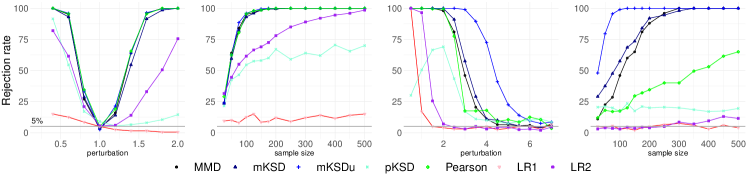
For both models, we investigate the performance of our test in two setting: perturbations from the null and increasing sample size, which we proceed to explain. Perturbations from the null: In this experiment, we investigate how the power changes for perturbations of the null hypothesis. For the Weibull data, we set and consider Weibull alternatives with . Notice that we recover the null hypothesis when . Also, we consider a constant of censored observations and a fixed sample size of . For the periodic experiment we set , which is recovered when we take tending to infinity. In this case, we consider alternatives . We consider, again, a constant of censoring, and a fixed sample size of . Increasing sample size: In this scenario, we investigate how the rejection rate of our test increases as the sample size increases. In the Weibull setting we set the null , the alternative as and in the periodic setting, we consider the null , and generate data from the alternative . In both settings we consider 30% of censored data points
Results
We show our results in Figure 2. For the Weibull data (first and second plots), observe that all kernel-based methods, except the pSKD, perform very similar to the Pearson test designed to perform extremely well in these types of setting. For the Periodic data (third and fourth plots), the goodness-of-fit problem is much more challenging, and we see differences in the performances of the methods. We observe that the MMD test of Fernandez and Gretton, [2019] has a better performance than the Pearson test, as was suggested by the experiments in their work. Our test mSKD performs slightly better than the the MMD test, whereas mSKDu outperform all the other methods by a huge margin. We can see that it is the most resistant to the increment in the perturbation parameter (third plot), and, for example, for , most methods cannot differentiate between null and alternative with large probability, whereas our method has power of around .
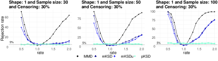
Proportionality
Our results show that pKSD is not a very powerful test. A possible explanation lies in the fact that, since this method tests against a model class, it must ignore all differences within this class, which affects the power of the test. Despite its lower power, it remains the only test out of the proposed methods that can test if our data was generated by a hazard proportional to . In Figure 3, we consider a Weibull hazard, given by , with shape and rate . Note that changing the parameter gives the same hazard up to a constant. Figure 3 shows that for a family of proportional hazards our method reaches the right type 1 error at low sample sizes, while all the other methods have non-trivial power. We observe, however, that for larger sample sizes, the test has a type-1 error that is slightly elevated over the design level. This may occur as the conditions of Theorem 8 are hard to satisfy in general, and have yet to be proven to hold for this case. Boostraping methods with strong theoretical guarantees under broader conditions are the subject of ongoing research.
Real Data Experiments
Data Sources
We perform our tests on the following real datasets to check relevant model assumptions. aml: Acute Myelogenous Leukemia survival dataset [Miller Jr,, 2011]; cgd: Chronic Granulotamous Disease dataset [Fleming and Harrington,, 2011]; ovarian: Ovarian Cancer Survival dataset [Edmonson et al.,, 1979]; lung: North Central Cancer Treatment Group (NCCTG) Lung Cancer dataset [Loprinzi et al.,, 1994]; stanford: Stanford Heart Transplant Data [Crowley and Hu,, 1977]; nafld: Non-alcohol fatty liver disease (NAFLD) [Allen et al.,, 2018].
Test Results
We apply our proposed tests on real dataset for the Testing hazard proportionality and Goodness-of-fit settings. First, we check model class assumption using pKSD to test whether the observed data is from a desired family model without fitting model parameters. We check the exponential model class and the Weibull model with shape=2. As the results shown in Table 1, our tests does not reject the Exponential model, which is coherent with scientific domain knowledge from the literature.111High-grade serous ovarian carcinoma (HG-SOC) is a major cause of cancer-related death. The growth of HG-SOC acts as an indicator of survival time of ovarian cancer [Gu et al.,, 2019]. This paper also suggests that HG-SOC follows exponential expansion, which implies exponentially distributed survival time of ovarian patient.
For the Goodness-of-fit test setting, we fit a cox proportional hazard model from the covariates provided in the datasets. The cox-proportional hazard function has the form , where is the base hazard and is the covariate for subject . The procedure is done via spliting the data into training set and test sets. Fitting the cox proportional-hazard model is applied on the training sets and the test sets are used to perform the goodness-of-fit tests. Results in Table 2 shows that all the models does not reject the fitted cox proportional hazard models and validate the proportional hazard assumptions for relevant fitted models, which is coherent with scientific experience stated in the literature.222 Chansky et al., [2016] suggests that cox proportional hazard model is a reasonable tool among practitioners for lung dataset. [Crowley and Hu,, 1977] suggests a fit for cox proportional hazard model for stanford dataset. Allen et al., [2018] states that cox proportional hazards is often used to study the impact of NAFLD on incident metabolic syndrome or death.
| p-value | aml | cgd | ovarian |
|---|---|---|---|
| Exponential | 0.585 | 0.460 | 0.681 |
| Weibull: shape=2 | 0.001 | 0.002 | 0.063 |
| Dataset | Covarites | p-value |
|---|---|---|
| lung | Age | 0.167 |
| stanford | T5 mismatch score | 0.594 |
| nafld | Weight and Gender | 0.108 |
Appendix
Appendix A Proofs and Derivations
A.1 Proofs of Section 3.1: Survival Stein Operator
A.1.1 Proof of Proposition 2
Let . Then
| (A.1) |
Observe that
therefore, the RHS of Equation (A.1) is equal to
Finally, the last expectation is 0 due to the identity , which follows from a simple computation.
A.1.2 Proof of Proposition 3
By definition,
We continue by proving that the previous norm converges to zero in probability. Observe that by the symmetrization lemma [Vershynin,, 2018, Lemma 6.4.2], it holds
where are i.i.d. Rademacher random variables, independent of the data . Then, by Jensen’s inequality, and by using that , we conclude that the previous expression converges to zero in probability, as
a.s., where the limit result holds due the law of large numbers which can be applied under the Condition in Equation (3.7) and since , as
A.2 Proofs of Section 3.3: Proportional Stein Operator
Proof of Propositon 4
We start by claiming that the following equation holds true for every :
| (A.2) |
Then, the main result follows from Equation (A.2), by using the law of large numbers and that
which follows from the definition of our operator (see Equation (3.13)).
We finish the proof by proving our claim in Equation (A.2). Observe that
| (A.3) |
where holds under the null hypothesis. We proceed to prove that the previous sum tends to in probability when grows to infinity. Let and define as the infimum of all such that . Notice that such is well-defined since . We continue by splitting the sum in Equation (A.3) into two regions, and , obtaining that Equation (A.3) equals
| (A.4) |
and we prove that both sums tend to 0 in probability when grows to infinity. We start with the first term. Observe that
where the previous result holds since almost surely by the Glivenko-Cantelli Theorem, and since
where the last expression is finite due to Equation (3.12).
Next, we deal with the second term in equation (A.4). Theorem 3.2.1. of Gill, [1980] yields , where , and, Lemma 2.7 of Gill, [1983] yields (recall that ). From the previous results, we get
Now, notice that
where the first equality holds by Equation (2.4), and the last inequality comes from the definition of . Since we can choose as small as desired, we conclude the result.
A.3 Proofs Section 4: Censored-Data Kernel Stein Discrepancy
A.3.1 Proof of Proposition 5
Proof.
Notice that, by the definition of the random function , we have that . Also notice that, for each fixed , and that the expectation, if and only if equation (4.1) is satisfied (the previous expectation has to be understood in the Bochner sense, as we are taking expectation of a random function).
Then,
where the third equality is due to the linearity of expectation and the inner product, the fourth equality follows from the definition of norm (and since we are taking supremum in the unit ball), and the second to last equality is, again, due to the linearity of the expectation and inner product. ∎
A.3.2 Explicit computation of
Denote , and , and . For simplicity of exposition, we will drop the superindex in all cases.
Survival Stein operator
: For this case, we have
Notice that a simple computation shows that , then
Martingale Stein operator
: Observe that in this case
Then, by the reproducing kernel property
Proportional Stein operator
: Notice that, in this case, we use , given in Equation (16), to compute since is not available, as it depends on , which is unknown even under the null hypothesis. Then,
Define . Then, by the reproducing kernel property,
Recall that denotes the risk function, which depends on all the data points, hence we write to recall the reader that this kernel is a random one.
A.4 Proofs of Section 5: Goodness-of-fit via c-KSD
The following lemmas show that, under Conditions c) and d) (depending on which case), the kernels have finite first and second moment. These moment conditions on the kernel are important to deduce asymptotic results.
Lemma 9.
Let and be independent samples from , and assume that Condition holds. Then,
for , under the alternative hypothesis.
Lemma 10.
Let and be independent samples from , and assume that Condition holds. Then
for , under the null hypothesis.
Proof of Lemma 9.
First of all, note that for any kernel (positive-definite function), it holds
hence, it is enough to only prove the first part of the lemma.
Survival Stein operator : Recall , where , then
The first and third term in the previous equation are finite under the technical Conditions a) and b). Thus, we only need to check
which is guaranteed by Condition d).
Martingale Stein operator : Recall that , where and . Then
Observe that the second and third term are finite under Condition a). Additionally, define and notice that
holds under Condition d) (Notice that in Condition d.2)).
Proportional Stein operator (). This case follows directly from Condition d.3). ∎
A.4.1 Proof of Theorem 6
We distinguish between two cases: first, when is a deterministic kernel (that is ), and second, when is a random kernel, meaning .
Deterministic kernel :
For the first case, we have
which is a V-statistic of order 2. Thus, by using the law of large numbers for V-statistics, we deduce
as n grows to infinity. Notice that the previous limit result requires the following conditions: and , which are satisfied under Condition d) by Lemma 9.
Random kernel :
For the second case, recall that
| (A.5) |
where is a random kernel. Our first step will be to assume that we can replace the random kernel , given by , by its limit , where . We claim that
| (A.6) |
and then we have that
where the third equality is due to the standard law of large numbers for V statistics, and by Condition d.3) and Lemma 9.
We finish the proof by proving the claim made in Equation (A.6). Recall that
and
| (A.7) |
where and Then, by the triangular inequality, and by taking square (notice that ), the claim in Equation (A.6) follows from proving:
-
i)
, and
-
ii)
Notice that item ii) holds trivially by Equation (A.7), and by the law of large numbers for V-statistics, which can be applied due to Lemma 9, under Condition d). We finish by proving the result in item i). Following the same steps used in Equation (A.3), we have that
| (A.8) | ||||
| (A.9) |
where and , and is the infimum over all such that
Notice that such a is well-defined by Lemma 9 and Condition d.3). For the term in Equation (A.8), observe that
| (A.10) | |||
| (A.11) |
where the last line holds since a.s., by an application of Glivenko-Cantelli, and since the double sum converges to
which is finite by Lemma 9 and Condition d.3).
Finally, we prove that the term in Equation (A.9) is . Define . Gill, [1983] proved that where . By using this result, the term in Equation (A.9) satisfies
where in the second line we used that , and in the fourth line we used the law of large numbers, and the definition of . Since is arbitrary, we conclude that equation (A.9) tends to 0 in probability.
A.4.2 Proof of Theorem 7
Survival Stein operator (c=s):
We proceed by contradiction. Assume that but . Recall that
Similarly, define
and notice that by the Stein’s identity. Then
and thus, we have
where , and where we identify as the mean kernel embedding of the measure . We shall assume that the above embedding is well-defined, otherwise we have . Since the kernel is -universal, the previous set of equations implies is the zero measure, which implies that , and
| (A.12) |
as long as implies (which does, since we assume implies ). Equation (A.12) yields and since both, and , are probability density functions. This finalizes our proof.
Martingale Stein operator (c=m):
Define
and notice that follows from the martingale identity. Observe that
Denote , and, as usual, . Then,
Since is -universal by Condition a), the previous term is equal to if and only if for all . Now, if and only if , which holds if and only if for all .
A.4.3 Proof of Theorem 8
Deterministic kernels :
For which are associated to a deterministic kernel function , the result follows from the classical theory of V-statistics since are degenerate kernels, and under the following moment conditions:
-
i)
, and
-
ii)
,
which are satisfied due to Lemma 10.
Random kernel :
Observe that
where . By hypothesis, for all , then
where . Therefore we conclude that , where
We will prove that . Let , then
where the two inequalities above follow from the Cauchy-Schwarz inequality, by the fact that [Yang,, 1994], and the previous double integral converges to 0 by Condition c.3), since . From the previous result, we deduce
The previous step is important in our analysis as it allows us to write in terms of . Our next step is to prove that we can replace the term , in the previous equation, by . Observe
The notation above denotes lower, given by , and upper, given by , bounds for . Finally, by taking square, the result is deduced by proving
and
The second equation won’t be verified as, at the end of this proof, we will show that such a quantity converges in distribution to some random variable, thus it will be bounded in probability. For the first equation, notice that
is a double integral with respect to the . Then, by Theorem 17 of Fernandez and Rivera, [2019], it is enough to verify
Observe that
where the second equality follows from uniformly for all [Gill,, 1983], and the last equality is due to dominated convergence in sets of probability as high as desired, as for all from the Glivenko Cantelli Theorem, and
which is integrable by Condition c.3).
Putting everything together, we have shown that
where . Notice that the process only depends on the -th observation . Notice that the previous expression is approximately a V-statistic with kernel given by . By proposition 23 of Fernandez and Rivera, [2019], we have that , thus is a degenerate V-statistic kernel.
By the classical theory of V-statistics,
where is a constant and is a (potentially) infinite sum of independent random variables, as long as the following moment conditions are satisfied:
Again, by Proposition 23 of Fernandez and Rivera, [2019], checking those moment conditions is equivalent to verify:
which are exactly the conditions assumed in Condition c.3).
Appendix B Known Identities
In Section 3.2, to derive the martingale Stein operator, we use the following identity
which holds under the null hypothesis, where is the hazard function under the null.
Let and be the individual counting and risk processes, defined by by and , respectively. Then, the individual zero-mean martingale for the i-th individual corresponds to , where for all .
Additionally, let such that for all , then is a zero-mean -martingale (See Chapter 2 of [Aalen et al.,, 2008]). The, taking expectation, we have
Appendix C Additional Experiments
C.1 Weibull experiments: small deviations from the null
Sample size: 30, and censoring percentages of , and
![[Uncaptioned image]](/html/2008.08397/assets/x4.png)
![[Uncaptioned image]](/html/2008.08397/assets/x5.png)
![[Uncaptioned image]](/html/2008.08397/assets/x6.png)
Sample size: 50, and censoring percentages of , and
![[Uncaptioned image]](/html/2008.08397/assets/x7.png)
![[Uncaptioned image]](/html/2008.08397/assets/x8.png)
![[Uncaptioned image]](/html/2008.08397/assets/x9.png)
Sample size: 100, and censoring percentages of , and
![[Uncaptioned image]](/html/2008.08397/assets/x10.png)
![[Uncaptioned image]](/html/2008.08397/assets/x11.png)
![[Uncaptioned image]](/html/2008.08397/assets/x12.png)
Sample size: 200, and censoring percentages of , and
![[Uncaptioned image]](/html/2008.08397/assets/x13.png)
![[Uncaptioned image]](/html/2008.08397/assets/x14.png)
![[Uncaptioned image]](/html/2008.08397/assets/x15.png)
C.2 Weibull experiments: increasing sample size
Shape: and censoring percentages of and
![[Uncaptioned image]](/html/2008.08397/assets/x16.png)
![[Uncaptioned image]](/html/2008.08397/assets/x17.png)
Shape: and censoring percentages of and
![[Uncaptioned image]](/html/2008.08397/assets/x18.png)
![[Uncaptioned image]](/html/2008.08397/assets/x19.png)
C.3 Periodic experiments: small deviations from the null
Sample size: 30, and censoring percentages of , and
![[Uncaptioned image]](/html/2008.08397/assets/x20.png)
![[Uncaptioned image]](/html/2008.08397/assets/x21.png)
![[Uncaptioned image]](/html/2008.08397/assets/x22.png)
Sample size: 50, and censoring percentages of , and
![[Uncaptioned image]](/html/2008.08397/assets/x23.png)
![[Uncaptioned image]](/html/2008.08397/assets/x24.png)
![[Uncaptioned image]](/html/2008.08397/assets/x25.png)
Sample size: 100, and censoring percentages of , and
![[Uncaptioned image]](/html/2008.08397/assets/x26.png)
![[Uncaptioned image]](/html/2008.08397/assets/x27.png)
![[Uncaptioned image]](/html/2008.08397/assets/x28.png)
Sample size: 200, and censoring percentages of , and
![[Uncaptioned image]](/html/2008.08397/assets/x29.png)
![[Uncaptioned image]](/html/2008.08397/assets/x30.png)
![[Uncaptioned image]](/html/2008.08397/assets/x31.png)
C.4 Periodic experiments: increasing sample size
Frequency: and censoring percentages of and
![[Uncaptioned image]](/html/2008.08397/assets/x32.png)
![[Uncaptioned image]](/html/2008.08397/assets/x33.png)
Frequency: and censoring percentages of and
![[Uncaptioned image]](/html/2008.08397/assets/x34.png)
![[Uncaptioned image]](/html/2008.08397/assets/x35.png)
References
- Aalen et al., [2008] Aalen, O., Borgan, O., and Gjessing, H. (2008). Survival and event history analysis: a process point of view. Springer Science & Business Media.
- Akritas, [1988] Akritas, M. G. (1988). Pearson-type goodness-of-fit tests: the univariate case. Journal of the American Statistical Association, 83(401):222–230.
- Allen et al., [2018] Allen, A. M., Therneau, T. M., Larson, J. J., Coward, A., Somers, V. K., and Kamath, P. S. (2018). Nonalcoholic fatty liver disease incidence and impact on metabolic burden and death: a 20 year-community study. Hepatology, 67(5):1726–1736.
- Andersen et al., [2012] Andersen, P. K., Geskus, R. B., de Witte, T., and Putter, H. (2012). Competing risks in epidemiology: possibilities and pitfalls. International journal of epidemiology, 41(3):861–870.
- Barbour and Chen, [2005] Barbour, A. D. and Chen, L. H. Y. (2005). An introduction to Stein’s method, volume 4. World Scientific.
- Biswas et al., [2007] Biswas, A., Datta, S., Fine, J. P., and Segal, M. R. (2007). Statistical advances in the biomedical science. Wiley Online Library.
- Bradburn et al., [2003] Bradburn, M. J., Clark, T. G., Love, S. B., and Altman, D. G. (2003). Survival analysis part ii: multivariate data analysis–an introduction to concepts and methods. British journal of cancer, 89(3):431–436.
- Brendel et al., [2014] Brendel, M., Janssen, A., Mayer, C.-D., and Pauly, M. (2014). Weighted logrank permutation tests for randomly right censored life science data. Scandinavian Journal of Statistics, 41(3):742–761.
- Chansky et al., [2016] Chansky, K., Subotic, D., Foster, N. R., and Blum, T. (2016). Survival analyses in lung cancer. Journal of thoracic disease, 8(11):3457.
- Chen et al., [2010] Chen, L. H. Y., Goldstein, L., and Shao, Q. M. (2010). Normal approximation by Stein’s method. Springer.
- Chung et al., [1991] Chung, C.-F., Schmidt, P., and Witte, A. D. (1991). Survival analysis: A survey. Journal of Quantitative Criminology, 7(1):59–98.
- Chwialkowski et al., [2016] Chwialkowski, K., Strathmann, H., and Gretton, A. (2016). A kernel test of goodness of fit. In Proceedings of the 33rd International Conference on International Conference on Machine Learning-Volume 48, pages 2606–2615.
- Collett, [2015] Collett, D. (2015). Modelling survival data in medical research. Chapman and Hall/CRC.
- Crowley and Hu, [1977] Crowley, J. and Hu, M. (1977). Covariance analysis of heart transplant survival data. Journal of the American Statistical Association, 72(357):27–36.
- Dehling and Mikosch, [1994] Dehling, H. and Mikosch, T. (1994). Random quadratic forms and the bootstrap for u-statistics. Journal of Multivariate Analysis, 51(2):392–413.
- Edmonson et al., [1979] Edmonson, J. H., Fleming, T. R., Decker, D., Malkasian, G., Jorgensen, E., Jefferies, J., Webb, M., and Kvols, L. (1979). Different chemotherapeutic sensitivities and host factors affecting prognosis in advanced ovarian carcinoma versus minimal residual disease. Cancer treatment reports, 63(2):241–247.
- Fernandez and Gretton, [2019] Fernandez, T. and Gretton, A. (2019). A maximum-mean-discrepancy goodness-of-fit test for censored data. In The 22nd International Conference on Artificial Intelligence and Statistics, pages 2966–2975.
- Fernandez et al., [2019] Fernandez, T., Gretton, A., Rindt, D., and Sejdinovic, D. (2019). A kernel log-rank test of independence for right-censored data. arXiv preprint arXiv:1912.03784.
- Fernandez and Rivera, [2019] Fernandez, T. and Rivera, N. (2019). A reproducing kernel hilbert space log-rank test for the two-sample problem. arXiv preprint arXiv:1904.05187.
- Fleming and Harrington, [2011] Fleming, T. R. and Harrington, D. P. (2011). Counting processes and survival analysis, volume 169. John Wiley & Sons.
- Gill, [1983] Gill, R. (1983). Large sample behaviour of the product-limit estimator on the whole line. Ann. Statist., 11(1):49–58.
- Gill, [1980] Gill, R. D. (1980). Censoring and stochastic integrals, volume 124 of Mathematical Centre Tracts. Mathematisch Centrum, Amsterdam.
- Gorham and Mackey, [2015] Gorham, J. and Mackey, L. (2015). Measuring sample quality with stein’s method. In Advances in Neural Information Processing Systems, pages 226–234.
- Gorham and Mackey, [2017] Gorham, J. and Mackey, L. (2017). Measuring sample quality with kernels. In ICML, pages 1292–1301.
- Gretton et al., [2012] Gretton, A., Borgwardt, K., Rasch, M., Schoelkopf, B., and Smola, A. (2012). A kernel two-sample test. JMLR, 13:723–773.
- Gu et al., [2019] Gu, S. S., Lheureux, S., Sayad, A., Cybulska, P., Hogen, L. B.-D., Vyarvelska, I., Tu, D., Parulekar, W., Levine, D. A., Bernardini, M. Q., et al. (2019). Computational modeling of ovarian cancer: Implications for therapy and screening. medRxiv, page 19009712.
- Hollander and Proschan, [1979] Hollander, M. and Proschan, F. (1979). Testing to determine the underlying distribution using randomly censored data. Biometrics, pages 393–401.
- Hyvärinen, [2005] Hyvärinen, A. (2005). Estimation of non-normalized statistical models by score matching. Journal of Machine Learning Research, 6(Apr):695–709.
- Jitkrittum et al., [2017] Jitkrittum, W., Xu, W., Szabó, Z., Fukumizu, K., and Gretton, A. (2017). A linear-time kernel goodness-of-fit test. In Advances in Neural Information Processing Systems, pages 262–271.
- Kanagawa et al., [2019] Kanagawa, H., Jitkrittum, W., Mackey, L., Fukumizu, K., and Gretton, A. (2019). A kernel stein test for comparing latent variable models. arXiv preprint arXiv:1907.00586.
- Kaplan and Meier, [1958] Kaplan, E. L. and Meier, P. (1958). Nonparametric estimation from incomplete observations. Journal of the American statistical association, 53(282):457–481.
- Klein and Moeschberger, [2006] Klein, J. P. and Moeschberger, M. L. (2006). Survival analysis: techniques for censored and truncated data. Springer Science & Business Media.
- Ley et al., [2017] Ley, C., Reinert, G., Swan, Y., et al. (2017). Stein’s method for comparison of univariate distributions. Probability Surveys, 14:1–52.
- Liu et al., [2016] Liu, Q., Lee, J., and Jordan, M. (2016). A kernelized stein discrepancy for goodness-of-fit tests. In International Conference on Machine Learning, pages 276–284.
- Loprinzi et al., [1994] Loprinzi, C. L., Laurie, J. A., Wieand, H. S., Krook, J. E., Novotny, P. J., Kugler, J. W., Bartel, J., Law, M., Bateman, M., and Klatt, N. E. (1994). Prospective evaluation of prognostic variables from patient-completed questionnaires. north central cancer treatment group. Journal of Clinical Oncology, 12(3):601–607.
- Miller Jr, [2011] Miller Jr, R. G. (2011). Survival analysis, volume 66. John Wiley & Sons.
- Mirabello et al., [2009] Mirabello, L., Troisi, R. J., and Savage, S. A. (2009). Osteosarcoma incidence and survival rates from 1973 to 2004: data from the surveillance, epidemiology, and end results program. Cancer: Interdisciplinary International Journal of the American Cancer Society, 115(7):1531–1543.
- Nelson, [1972] Nelson, W. (1972). Theory and applications of hazard plotting for censored failure data. Technometrics, 14(4):945–966.
- Vershynin, [2018] Vershynin, R. (2018). High-Dimensional Probability: An Introduction with Applications in Data Science. Cambridge Series in Statistical and Probabilistic Mathematics. Cambridge University Press.
- Xu and Matsuda, [2020] Xu, W. and Matsuda, T. (2020). A stein goodness-of-fit test for directional distributions. The 23rd International Conference on Artificial Intelligence and Statistics.
- Yang et al., [2018] Yang, J., Liu, Q., Rao, V., and Neville, J. (2018). Goodness-of-fit testing for discrete distributions via stein discrepancy. In International Conference on Machine Learning, pages 5557–5566.
- Yang et al., [2019] Yang, J., Rao, V., and Neville, J. (2019). A stein–papangelou goodness-of-fit test for point processes. In The 22nd International Conference on Artificial Intelligence and Statistics, pages 226–235.
- Yang, [1994] Yang, S. (1994). A central limit theorem for functionals of the Kaplan-Meier estimator. Statist. Probab. Lett., 21(5):337–345.