All good things come in threes: the third image of the lensed quasar PKS 1830$-$211

Strong gravitational lensing distorts our view of sources at cosmological distances but brings invaluable constraints on the mass content of foreground objects and on the geometry and properties of the Universe. We report the detection of a third continuum source toward the strongly lensed quasar PKS 1830$-$211 in ALMA multi-frequency observations of high dynamic range and high angular resolution. This third source is point-like and located slightly to the north of the diagonal joining the two main lensed images, A and B, $0.3\arcsec$ away from image B. It has a flux density that is $\sim 140$ times weaker than images A and B and a similar spectral index, compatible with synchrotron emission. We conclude that this source is most likely the expected highly de-magnified third lensed image of the quasar. In addition, we detect, for the first time at millimeter wavelengths, weak and asymmetrical extensions departing from images A and B that correspond to the brightest regions of the Einstein ring seen at centimeter wavelengths. Their spectral index is steeper than that of compact images A, B, and C, which suggests that they arise from a different component of the quasar. Using the GravLens code, we explore the implications of our findings on the lensing model and propose a simple model that accurately reproduces our ALMA data and previous VLA observations. With a more precise and accurate measurement of the time delay between images A and B, the system PKS 1830$-$211 could help to constrain the Hubble constant to a precision of a few percent.

1 Introduction

The theory of general relativity describes gravity as a geometric property of the space-time continuum. The presence of a mass changes the local curvature of the Universe and can bend the trajectory of photons, possibly leading to distorted images of background sources. Over cosmological distances, even a small deflection of the photons can result in a different path-length and an apparent time delay between lensed images, related to the Hubble constant, $H_{0}$. Gravitational lensing therefore offers a unique opportunity to assess mass distributions in the Universe and measure $H_{0}$ via the so-called time-delay cosmography method (Refsdal 1964 and, e.g., Wong et al. 2020 and results from the H0LiCOW collaboration).

The relative positions of the source, the lens, and the observer set the number of lensed images, their magnifications, and the time delays between them (e.g., Schneider et al. 1992). In the special geometrical case where the source, lens, and observer are closely aligned, the resulting image of the source is a perfect Einstein ring. More generally, a gravitational lens always produces an odd number of images, partially or well separated. One of them is always located close to the center of the lens and, in contrast to other images, is highly de-magnified (by a factor $\sim$10² to $10^{4}$). This central image brings important information: its position and de-magnification ratio can put strong constraints on the lens geometry (lens position, ellipticity of the dark matter halo) and on the lens central mass distribution (see e.g., Keeton 2003; Tamura et al. 2015; Wong et al. 2015).

Detections of the central image are rare and difficult (e.g., Winn et al. 2004; Quinn et al. 2016). They require high sensitivity in order to overcome the strong demagnification, high angular resolution in order to resolve the different components (typically separated by a few arcseconds in the sky), and high dynamic range ($>100-1000$). In addition, confusion can arise between the third image, that is, emission from the background source, and photons emitted by the lens itself. Finally, propagation effects (e.g., free–free absorption through the lens, or extinction and reddening due to dust) can also affect the observations.

The system PKS 1830$-$211 is a remarkable case of strong gravitational lensing. It consists of a radio-loud quasar at $z=2.5$ (Lidman et al. 1999), a foreground lens in the form of a nearly face-on $z=0.89$ spiral galaxy (Wiklind & Combes 1996; Winn et al. 2002; Koopmans & de Bruyn 2005) which is also responsible for remarkable molecular absorption (e.g., Wiklind & Combes 1996; Muller et al. 2011, 2014), and a second intervening galaxy at $z=0.19$ with H I and OH absorption (Lovell et al. 1996; Allison et al. 2017). However, this second galaxy is expected to have a negligible effect on the lensing (Winn et al. 2002; Sridhar 2013). The resulting image of the quasar appears at centimeter wavelengths as two highly magnified compact components (hereafter labeled images A and B, to the northeast and southwest, respectively) separated by $\sim 1\arcsec$ and embedded in a full Einstein ring (Subrahmanyan et al. 1990; Jauncey et al. 1991; Nair et al. 1993). Another component close to image B was tentatively identified as the third image by Nair et al. (1993).

Although many observations have been performed toward PKS 1830$-$211 at different wavelengths (radio, optical, X- and $\gamma$-rays), there has been so far no convergence toward a single lens model. One of the major sources of debate and uncertainty is the lens position (Table 4, see also, e.g., Sridhar 2013). PKS 1830$-$211 is located behind the Galactic plane, close to the direction of the Galactic Center ($b$=$-5.7^{\circ}$), meaning that optical observations suffer from high extinction by dust and contamination by Galactic stars, making a robust optical identification difficult (e.g., Winn et al. 2002; Courbin et al. 2002). In radio–cm observations, the third image is tentatively identified (component E by Subrahmanyan et al. 1990), with a flux density more than one hundred times lower than that of image A (Nair et al. 1993). However, the variability of PKS 1830$-$211 prevents the use of data obtained at different epochs, making it difficult to measure spectral indices to confirm the identification. In addition, there are some ambiguities in the radio–cm images with possible jet-knot extensions from image B. Similarly, very-long-baseline interferometric (VLBI) observations show strong intrinsic variability of the quasar images (Garrett et al. 1997; Guirado et al. 1999), making it difficult to disentangle the jet–core sub-components. The VLBI observations are also limited in terms of dynamic range, making it difficult to detect the faint third image.

Concerning measurements of the time delay between images A and B, several methods have been deployed with various success, from radio monitoring (van Ommen 1995; Lovell et al. 1998) to analysis of molecular absorption variations (Wiklind & Combes 2001) and $\gamma$-ray time-series (Barnacka et al. 2011; Abdo et al. 2015; Barnacka et al. 2015), with results pointing toward a most likely value of between 20 and 30 days. Finally, even the differential magnification ratio ($\mu_{\rm A}/\mu_{\rm B}$) is uncertain because the instantaneous flux density ratio A/B is varying with time due to the intrinsic variability of the quasar modulated by the time delay. Values in the range 1-2 have been observed (e.g., van Ommen 1995; Muller & Guélin 2008; Martí-Vidal et al. 2013, 2020). In principle, micro-lensing on one line of sight could also affect the ratio for some time (e.g., on a 1 year timescale).

Here, we report new millimeter observations with the Atacama Large Millimeter/submillimeter Array (ALMA) that allowed us to unambiguously identify the third image of PKS 1830$-$211 and refine the lens model of the system.

2 Observations

Our ALMA observations of PKS 1830$-$211 were carried out on 2019 July 10 and 11 in bands 4 ($\sim 150$ GHz) and 6 ($\sim 230$ GHz), and on 2019 July 28 in bands 5 ($\sim 180$ GHz) and 7 ($\sim 280$ GHz). The array was in an extended configuration, with longest baselines up to 8–14 km depending on the date. This resulted in a synthesized beam of between 60 mas and 20 mas. The largest recoverable angular scale (i.e., due to the filtering of extended emission by the interferometer) is larger than the extent of the Einstein ring, and therefore we do not expect to miss extended emission. A summary of the observations is given in Table 2.

The correlator was configured to cover four independent spectral windows, each of 1.875 GHz in width, with a spectral resolution $\sim 0.5$–1 MHz adapted for the study of the molecular absorption lines arising from the $z=0.89$ intervening lens galaxy (e.g., Muller et al. 2014). All the absorption features were flagged to image the continuum emission.

The data calibration was done within the CASA package, following a standard procedure. The bandpass response of the antennas was calibrated from observations of the bright quasar J 1924$-$292 (3.8 to 2.5 Jy with increasing frequency), which was also used for the absolute flux calibration. Conservatively, the flux accuracy is better than 5% at bands 4, 5, and 6, and better than 10% at band 7, as retrieved from the ALMA observatory flux monitoring data of J 1924$-$292 at the date of observations. The quasar J 1832$-$2039, $\sim 0.3$ Jy and about half a degree away from PKS 1830$-$211 in the sky, was observed every 5–7 min for gain (phase and amplitude) calibration.

After the standard calibration, the visibility phases were furthermore self-calibrated on the continuum of PKS 1830$-$211, applying phase-only gain corrections at each 6 s integration. This self-calibration step dramatically improved the quality of the data by reducing the atmospheric decoherence. In particular, the dynamic range (i.e., the ratio of peak flux to rms noise level in the image) improved by a factor of two to three after self-calibration, and reached values $\gtrsim 1000$, which is about the high-end expectation for ALMA observations . This is possible due to the strong flux density of the A and B images of PKS 1830$-$211, which allows us to derive self-calibration gain corrections on the shortest integration interval, although the dynamic range is still limited, for example, by antenna position uncertainties, potential residual calibration issues, and digit quantization in the correlator.

The final images of the continuum emission (Fig. 1) were produced for each band separately, from a Högbom-Clean multi-frequency synthesis deconvolution of the interferometric visibilities, with a pixel size of 5 mas.

3 Results

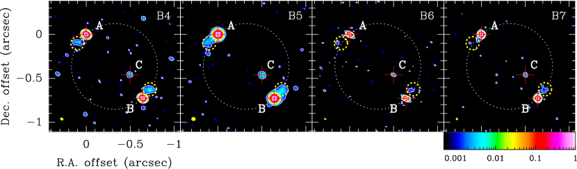
Figure 1: Continuum images of PKS 1830$-$211 obtained with ALMA in bands 4, 5, 6, and 7. Intensities are normalized to the peak of each image. The color wedge shown at the bottom of the extreme right box is the same for all images. Contour levels are drawn at 0.1%, 1%, and 50%. The positions of images A, B, and C are marked with red crosses. The weak extensions departing from images A and B are indicated by the yellow dashed circles. The center of the white dashed circle corresponds to the halfway point between images A and B. The synthesized beam is shown as the yellow ellipse in the bottom-left corner of each box.

The maps of PKS 1830$-$211 in the four observed ALMA bands (Fig. 1) reveal (i) the two images A and B, as two bright point-like sources, (ii) weak asymmetrical extensions departing from these images, to the southeast for image A and to the northwest for image B, and (iii) an additional faint and isolated third point-like source, hereafter denoted image C, located slightly north above the line joining images A and B, about 0.3$\arcsec$ away from image B. The positions and flux properties of the three images A, B, and C are listed in Table 1.

The location of the third point-like source, its flux ratio relative to images A and B, and its similar spectral index point toward its identification as the expected third, de-magnified lensed image of PKS 1830$-$211. We note that its position is consistent with “feature E” identified on the VLA maps by Subrahmanyan et al. (1990) and Nair et al. (1993), and with the deconvolved position of the lens galaxy by Meylan et al. (2005) (see Table 4). The ALMA identification of the third image finally removes any confusion around the nature of feature E and the position of the lens galaxy (Courbin et al. 2002; Winn et al. 2002; Meylan et al. 2005), hence allowing a major improvement of the lens model.

The weak extensions departing from images A and B are the counterparts of the brightest regions of the Einstein ring seen at centimeter wavelengths (Subrahmanyan et al. 1990). These are more conspicuous in ALMA bands 4 and 5 than in bands 6 and 7, and we estimate spectral indices $\alpha=-1.28\pm 0.15$ and $-1.18\pm 0.15$ toward A and B extensions, respectively. These spectral indices are significantly steeper than those of the point-like images A, B, and C, which indicates that the extensions correspond to a different source component. The extension departing from image B is about 1.4 times brighter than the one departing from image A. However, we note that the flux ratio of the extensions may vary with time in a way that is not necessarily related to the variations of the flux ratio of the images, A/B.

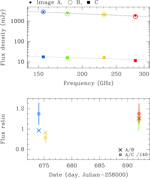
Figure 2: Flux density of the three images of PKS 1830$-$211 as a function of frequency and power-law fit of the spectral indices (top panel), and flux density ratios as a function of time (bottom panel). The color code is the same for both figures.

Table 1: Properties of the three lensed images of PKS 1830$-$211 from the ALMA 2019 data.

Image	R.A. offset	Dec. offset	Flux density at 300 GHz	Flux normalized	Spectral index
	(mas)	(mas)	(mJy)	to image A	$\alpha$
A	0.0	0.0	$1776\pm 36$	1.0	$-0.698\pm 0.045$
B	$-641.946\pm 0.042$	$-728.082\pm 0.033$	$1658\pm 165$	$0.93\pm 0.09$	$-0.79\pm 0.21$
C	$-500.1\pm 2.1$	$-459.6\pm 1.6$	$12.6\pm 1.6$	$0.0071\pm 0.0009$	$-0.53\pm 0.28$

4 Revising the lens model for PKS 1830$-$211

Armed with the new constraint of the unambiguous position of the third image, we can revise the lens model for PKS 1830$-$211. For this, we used the GravLens code (Keeton 2001) in successive steps, as described below.

First, we modeled the source and images as point-like objects, that is, ignoring the weak extensions. A softened isothermal ellipsoidal model was adopted for the lens mass distribution (e.g., Kormann et al. 1994 and see App. B.1). In addition to the redshifts of the source and lens, the lens model has therefore eight free parameters: the position of the (point-like) source and the position, scale mass, softening length, ellipticity, and position angle of the softened isothermal ellipsoidal lens. We took the position of the third image as an initial guess for the center of the lens, because both are expected to be very close. More details are given in Appendix B. The best-fit model was obtained by minimizing the $\chi$-square in the source and image plane, successively (see Keeton 2001). The values of input and output parameters are listed in Table 5. The outcome of the fit is shown in the form of Monte-Carlo degeneracy parameter plots (”corner plots”) in Fig. 5.

Our goal was not to achieve the ultimate modeling of the system, but to build one plausible model that could satisfy the existing VLA and ALMA observations, and in particular the new constraint imposed by the identification of the third image. As previously mentioned, we considered that we could neglect line-of-sight structures, starting with the second absorber at $z=0.19$ (see Appendix B.2).

We also refrained from trying to constrain the value of $H_{0}$, because there is currently no precise and accurate determination of the time delay $t_{\rm AB}$ . Instead, we ran the modeling with two values of $H_{0}$, the first one derived from Planck data (Planck coll. 2018) and the second from modeling strong gravitational lens systems (Wong et al. 2020). Those two values are close enough (although statistically in tension with each other) so that the corresponding time delays between the images do not differ by more than $\sim 10$%. Reciprocally, the exercise shows that a precise and accurate measurement of the time delays toward PKS 1830$-$211 could help constrain $H_{0}$ possibly to a precision of a few percent, although sources of systematic errors (such as line-of-sight structures, shear degeneracy, lens model choice, see, e.g., Wong et al. 2020; Millon et al. 2020) would have to be carefully explored, which is beyond the scope of this paper.

For the lens model to reproduce the weak extensions and, subsequently the Einstein ring seen at centimeter wavelengths, we have to add components to the source. Although the lensing is achromatic, these components (such as a core and a jet) may have different spectral indices, and therefore we may need to adopt different source models to reproduce the ALMA and VLA observations. First, keeping the same lens model as derived above, we considered two point-like images at the positions of the weak extensions seen by ALMA (center of the yellow dashed circles in Fig. 1), and searched for their corresponding point-like source in the source plane. We found that this second point-like source would fall at a position $(-333.33,-341.55)$ mas relative to image A, that is, a separation of 55 mas ($\sim 0.5$ kpc at the redshift of the quasar) and a position angle ${PA}=107^{\circ}$ (east of north) in the plane of the sky with respect to the original source of images A, B, and C. This simple model with just two point-like sources reproduces the ALMA observations well (Fig. 3a).

As a next step, we modeled the second source as an extended one by using a Sérsic intensity distribution profile, and played with GravLens using the VLA-15 GHz image of Subrahmanyan et al. (1990) (see Fig. 3c) as a visual guide. After several trials varying its positions, size, and Sérsic index, we found that a remarkable match between the VLA and GravLens model images (Fig. 3b) could be obtained simply by adopting a 1D Sérsic profile with Sérsic index $n=1$ (i.e., an exponential intensity distribution profile), centered at the same position as the second point-like source above, and with a half-light radius of 55 mas, equal to the separation between the two point-like sources of the ALMA model. Despite its elegant simplicity and minimum set of parameters, our model successfully reproduces all the features of PKS 1830$-$211: the three compact images, the asymmetrical extensions eventually forming the Einstein ring, and the bridge-like feature between images B and C seen in the VLA image.

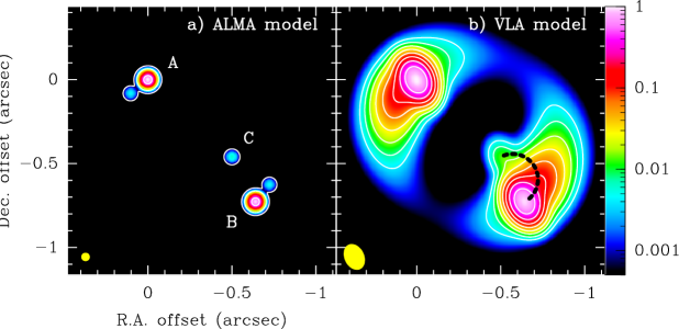
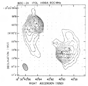
Figure 3: Results from the ALMA and VLA lens models (see Table 6). Images are normalized to the peak intensity and smoothed to the beam (shown in bottom-left corner) given hereafter. (a) ALMA model with two point-like sources, smoothed to a resolution of 30 mas. Contour levels at 0.5, 0.01, and 0.0005. (b) VLA model, with one point-like and one extended source, smoothed to the same beam as the VLA-15 GHz observations by Subrahmanyan et al. (1990): $161\times 117$ mas², with a position angle of 26^∘. Contour levels every 1/2ⁿ, with $n=1$ to 10. In our simulations, a thin jet would follow an arclet feature between images B and C, as indicated by the dashed curve. Right: VLA-15 GHz observations by Subrahmanyan et al. (1990). We note that their labels of the different features are not the same as ours: in this image, labels C and D mark the extensions from images A and B, and label E corresponds to the third image.

5 Discussion and perspectives

Our simple model points toward a core–jet morphology of the quasar, with a bright and compact ”core” producing the three point-like images A, B, and C, and a fainter ”jet” component, more extended at lower frequency, producing the extensions, the Einstein ring, and the bridge-like feature between images B and C (hereafter BC). At millimeter wavelengths, the core-jet separation ($\sim 55$  mas) as well as the core and jet sizes ($\ll 30$ mas) are well constrained by the high angular resolution of our ALMA observations. Also at VLA frequencies, the core-jet separation cannot be much more than $\sim 50$ mas: otherwise, the extension features would extend farther out from their respective main images A and B, and even become detached if we keep a size no larger than $\sim 50$ mas for the jet. An apparent detached jet could in fact be the signature of stationary bright spots in the jet, for instance due to recollimation shocks (e.g., Bromberg & Levinson 2009).

Image C is the third image of the core, and does not correspond to the jet. This is clearly set by the ALMA observations: at millimeter wavelengths, we do not expect to detect emission from the jet because of its steep spectral index and the strong de-magnification at the location of the third image. The bridge-like feature BC, on the other hand, is due to the extended jet. Indeed, according to our lensing model, a very thin and extended ($>0.15$ mas) jet source component toward $PA=107^{\circ}$ would form a complete ring-like feature in the image plane, roughly centered at the middle of segment BC and with a diameter equal to the separation BC. Hence, we hypothesize that the bridge-like feature BC corresponds to the northwestern part of this ring, which is brighter as it is more favorably magnified by the lens geometry.

From our model, we derive magnifications close to three for images A and B (with opposite parity) and a de-magnification by a factor $\sim 50$ for image C (with same parity as image A). However, it should be kept in mind that the observed flux density ratios, A/B and A/C, can be modulated by the intrinsic time variability of the quasar and the time delays by up to several tens of percent. The flux density ratio A/B has indeed been seen to vary between one and two (e.g., Muller & Guélin 2008; Martí-Vidal et al. 2013). Furthermore, a study of the time variations of all three images A, B, and C would bring additional evidence that C is the third image of the core.

The detection of the third image of PKS 1830$-$211, allowing us to refine the lens model of the system, opens up new perspectives:

• Our model predicts time delays of $t_{\rm AB}\sim 26-29$ days and $t_{\rm AC}\sim 31-34$ days, depending on $H_{0}$ (see Table 5). With a robust measurement of the time delay $t_{\rm AB}$, PKS 1830$-$211 could be used in a sample of strong gravitationally lensed systems to constrain $H_{0}$ (e.g., Wong et al. 2020).

• It would be interesting (although certainly challenging) to search for absorption toward the weak extensions and image C to obtain further insight into the content, distribution, and kinematics of the gas in the lens galaxy (e.g., Muller et al. 2014). This would help to constrain the properties of the galaxy, such as its inclination and disk rotation, which have so far only been investigated with unresolved H I absorption data (Koopmans & de Bruyn 2005).

• The time variability and polarization properties of the continuum emission have been used to study the different components of the quasar (e.g., Martí-Vidal et al. 2013; Martí-Vidal & Muller 2019; Martí-Vidal et al. 2020). A high-angular-resolution monitoring of PKS 1830$-$211 (e.g., with ALMA or mm-VLBI), resolving the third image and the jet extensions, would allow us to further characterize the structure of the jet.

Appendix A Additional information

Table 2: Summary of the observations.

Tuning	Frequency	Date	$N_{\rm ant}$	$B_{\rm min}$	$B_{\rm max}$	PWV	$t_{\rm on}$	Beam / P.A.	LRAS
	(GHz)			(m)	(km)	(mm)	(min)	(mas $\times$ mas / deg)	($\arcsec$)
B4	154.89	2019 Jul 10	45	138	13.9	2.1	7:36	$46.9\times 37.7$ / 61.5	1.4
B5	181.40	2019 Jul 28	43	92	8.5	0.6	17:14	$56.4\times 51.6$ / 87.0	1.8
B6	230.89	2019 Jul 11	44	111	12.6	1.2	24:52	$37.5\times 23.2$ / 70.0	1.2
B7	283.38	2019 Jul 28	42	92	8.5	0.6	18:49	$34.3\times 32.9$ / 42.3	1.2

Table 3: Flux density ratios measured during the different ALMA observations in July 2019.

Date	Band	$f_{\rm A}$ (Jy)	A/B	A/C
10/07/2019	B4	2.85	$0.986\pm 0.002$	$161\pm 15$
11/07/2019	B6	2.13	$0.965\pm 0.002$	$128\pm 7$
28/07/2019	B5	2.48	$1.097\pm 0.002$	$152_{-11}^{+14}$
28/07/2019	B7	1.89	$1.109\pm 0.002$	$161\pm 14$

Table 4: Astrometry of sources in the field of PKS 1830$-$211.

Reference	Instrument	Position relative to image A ($-$R.A., $-$Dec. offsets, mas) (a)
		Image B	Others
Lehár et al. (2000)	HST (K,H,I)	(653, 721) $\pm 1$	lens G: (501, 445) $\pm 80$
Courbin et al. (2002)	HST & Gemini	(654, 725) $\pm 2$	lens G: (519, 511) $\pm 80$
	(V,I,K)		SP: (285, 722) $\pm 40$
Winn et al. (2002)	HST (V,I)		lens G: (328, 486) $\pm 4$
Meylan et al. (2005)	VLT (J,H,Ks)	(649, 724) $\pm 1$	lens G: (498, 456) $\pm 4$
			star P: (333, 504) $\pm 2$
Jin et al. (2003)	VLBA (43 GHz)	(642.092, 728.086) $\pm 0.2$(systematics) (b)
This work	ALMA	(641.946 $\pm 0.042$, 728.082 $\pm 0.033)$	C: (500.1 $\pm 2.1$, 459.6 $\pm 1.6$)

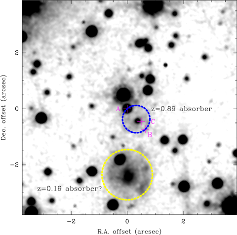
Figure 4: I-band image of the surrounding of PKS 1830$-$211 obtained from the Hubble Space Telescope Archive (WFPC2, F814W; see also publications by Winn et al. 2002; Courbin et al. 2002). The three images, A, B, and C, are marked with magenta crosses. The dashed yellow circle shows the location of the candidate $z=0.19$ H I/OH absorber, about $2.5\arcsec$ south of image A.

Appendix B Fitting the lens model

B.1 The $z=0.89$ lens

The lensed images of a source are the solutions to the lens equation, given the configuration of source and lens positions, and lens potential:

$${\bf u}={\bf x}-\alpha({\bf x}),$$ (1)

where u and x are the source and images positions (i.e., 2D vectors on the plane of the sky), respectively, and $\alpha$ is the deflection angle due to the 2D gravitational potential $\phi$ of the lens:

$$\alpha({\bf x})=\nabla\phi({\bf x}).$$ (2)

The potential is linked to the dimensionless convergence $\kappa$:

$$\nabla^{2}\phi({\bf x})=2\kappa({\bf x}),$$ (3)

which is defined as the surface density of the lens $\Sigma({\bf x})$ in units of the critical surface density $\Sigma_{cr}$ of the system:

$$\Sigma_{cr}=\frac{c^{2}}{4\pi G}\frac{D_{os}}{D_{ol}D_{ls}}.$$ (4)

There, $D_{os}$ is the angular distance between the observer and the source, $D_{ol}$, the angular distance between the observer and the lens, and $D_{ls}$, the angular distance between the lens and the source. In the case of the PKS 1830$-$211 system (with a flat Universe defined by $\Omega_{m}=0.3$ and $\Omega_{\Lambda}=0.7$), we get $\Sigma_{cr}=2.24\times 10^{9}$ M_⊙ kpc^-2.

For the lens mass model, we adopt a softened isothermal ellipsoidal (see, e.g., Kormann et al. 1994):

$$\kappa(x^{\prime},y^{\prime})=\frac{\mathcal{M}}{2}\left[s^{2}+x^{\prime 2}+\frac{y^{\prime 2}}{1-e^{2}}\right]^{-\frac{1}{2}},$$ (5)

where $\mathcal{M}$ is a mass scale, $s$ is the softening length, and $e$ is the ellipticity, with the coordinate axes $(x^{\prime},y^{\prime})$ centered on the lens with a position angle $\theta$.

Because the redshifts of the lens and source are observationally set, there are six free parameters left for the lens ($x_{l}$, $y_{l}$, $\mathcal{M}$, $s$, $e$, and $\theta$), which can be solved from the relative positions of the three lensed images. The best-fit values of those parameters are given in Table 5. Corner plots are shown in Fig. 5.

From the monopole deflection for our lens model, we can calculate the mass enclosed within a given radius, which we find to be $\sim 4\times 10^{11}$ M_⊙ within a region of $1\arcsec$ in diameter (i.e., $\sim 7.4$ kpc) centered on the lens. Within a radius of 40 kpc, we estimate a total enclosed mass of roughly $9\times 10^{11}$ M_⊙. As expected, the position of the lens center is very close ($<20$ mas) to that of the third image.

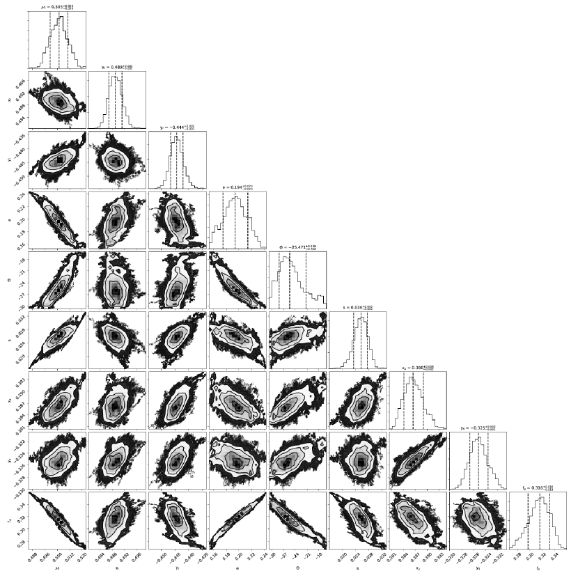
Figure 5: Plots showing the parameter degeneracies from the GravLens Monte-Carlo fitting with a single point-like source. $x_{s}$ and $y_{s}$ are the position of the source (in arcsec), with respect to image A, and $f_{s}$ its flux normalized to that of image A. $x_{l}$ and $y_{l}$ are the positions of the center of the adopted softened isothermal ellipsoidal model (in arcsec), $e$ is the ellipticity, and $\theta$ the position angle (in degrees). $\mathcal{M}$ is the mass scale and $s$ the softening length (see Eq. 5), both in arcsec.

Table 5: Input parameters and results of the GravLens model fitting of the lens.

Input parameters
Cosmology	$\Omega_{m}$, $\Omega_{\Lambda}$	0.3, 0.7
	$H_{0}$ (km s-1 Mpc-1)	67.4$\pm$0.5; $73.3_{-1.8}^{+1.7}$		(1)
Source	Redshift $z_{S}$	2.507		(2)
	Intensity profile	point-like
Lens	Redshift $z_{L}$	0.88582		(3)
	Initial guess position	-500.1, -459.6		(4)
	Mass distribution	softened isothermal ellipsoidal
Lensed images	Position of image A	$(\Delta{\rm RA},\Delta{\rm Dec})\equiv(0,0)$		(5)
	Position of image B (mas)	$-641.946\pm 0.042,-728.082\pm 0.033$		(6)
	Position of image C (mas)	$-500.1\pm 2.1,-459.6\pm 1.6$		(6)
	Flux ratios (A:B:C)	$1:0.93\pm 0.09:0.0071\pm 0.0009$		(7)
Output parameters
		Best fit	Guess range
Source	Position $x_{s},y_{s}$ (mas)	$-386\pm 3,-325\pm 2$		(8)
	Flux $f_{s}$	$0.317\ ^{+0.016}_{-0.019}$		(9)
Lens	Position $x_{l},y_{l}$ (mas)	$-489\pm 2,-444\pm 2$		(8)
	Mass scale (mas)	$505\pm 6$	[100; 1500]	(10)
	Softening length $s$ (mas)	$26\pm 2$	[10; 200]	(10)
	Ellipticity $e$	$0.19\pm 0.02$	[0.0; 0.3]
	Position angle $\theta$ (∘)	$-25\ ^{+4}_{-3}$	[$-90$;+90]
Derived quantities
Time delay	$t_{\rm AB}$ (d)	28.6; 26.3		(11)
	$t_{\rm AC}$ (d)	33.7; 31.0		(11)
Magnification	$\mu_{\rm A}$	3.1
	$\mu_{\rm B}$	$-2.9$
	$\mu_{\rm C}$	$0.022$

B.2 The second absorber at $z=0.19$

There is a second absorber at a redshift $z=0.19$ in the line of sight of PKS 1830$-$211, detected in H I and OH absorption, first by Lovell et al. (1996) and re-observed more recently by Allison et al. (2017). The closest galaxy in the immediate surroundings of PKS 1830$-$211 is located about $2.5\arcsec$ south of image A, as can be seen in the HST image shown in Fig. 4 (see also Lehár et al. 2000; Winn et al. 2002; Courbin et al. 2002; Meylan et al. 2005 for analysis and discussion of optical images of PKS 1830$-$211). To our knowledge there is no spectroscopic confirmation that this galaxy is indeed the second absorber but there are no other obvious candidates. The galaxy is brighter than the $z=0.89$ galaxy and has a larger angular size, and its photometry is consistent with that of a relatively nearby spiral (Winn et al. 2002).

We can calculate the convergence $\kappa^{\prime}$ due to an object at the location of this second galaxy for a range of redshift and mass. Assuming a singular isothermal sphere model for the new lens galaxy with 1D stellar dispersion $\sigma_{v}$, we have

$$\kappa^{\prime}(\theta)=\frac{2\pi\sigma_{v}^{2}}{c^{2}}\frac{D_{ls}}{D_{os}}\frac{1}{\theta},$$ (6)

where $\theta$ is the angular distance between the new lens and a given location. We find that its lensing effect is negligible at the location of both images A and B (slightly larger at image B because it is closer in the sky to the second galaxy), with $\kappa^{\prime}<1$ (and decreasing with increasing redshift of the object) as long as its stellar dispersion $\sigma_{v}<350$ km s^-1. For $z=0.2$ and $\sigma_{v}=200$ km s^-1, $\kappa^{\prime}=0.3$ at image B. Therefore, only a nearby and very massive galaxy could introduce some weak lensing effect.

B.3 The source

The first lens model was derived considering a single point-like source $S_{1}$ at the origin of the three compact lensed images A, B, and C. To account for the extensions, one needs to add source components.

To reproduce the weak and compact extensions seen on the ALMA observations, we simply added one more point-like component $S_{2}$ (in practice a Sérsic intensity profile with a very small half-light radius of 1 mas), and found that it should be set at a position 55 mas with a position angle ($PA$) of 107^∘ with respect to the first source $S_{1}$.

To further reproduce the partial Einstein ring as mapped with the VLA (e.g., Subrahmanyan et al. 1990), we need to move the second source into an extended component $S_{2}^{\prime}$, for example using a Sérsic intensity profile. A simple but remarkably good solution was found by setting $S_{2}^{\prime}$ at the same position as $S_{2}$, using a 1D Sérsic profile with a half-light radius of 55 mas (i.e., the distance between $S_{1}$ and $S_{2}$), and a Sérsic index $n=1$, i.e., corresponding to an exponential profile (Table 6). To account for the sharp cut in emission to the northwest of image A and southeast of image B in the VLA images, one should suppress emission opposite to the jet. However, the match between our model and the observations is already more than satisfying for the purpose of this study, especially given the simplicity (small number of parameters) of our model. This is also why we refrained from exploring further ellipsoidal (2D) Sérsic intensity profiles for the extended source.

The parameters of the ALMA and VLA source models (Fig. 3) are given in Table 6.

Table 6: Parameters of the Sérsic intensity profiles used for the ALMA and VLA source models (Fig. 3a and b, respectively).

		(X,Y) (a)	$r_{0}$ (b)	$I_{0}$ (c)	$n$ (d)
		(mas)	(mas)
ALMA model	$S_{1}$	$(-386,-325)$	1	1	1
	$S_{2}$	$(-333,-341)$	1	0.005	1
VLA model	$S_{1}$	$(-386,-325)$	1	1	1
	$S_{2}^{\prime}$	$(-333,-341)$	55	0.5	1