Dark soliton-like magnetic domain walls in a two-dimensional ferromagnetic superfluid

Abstract

We report a stable magnetic domain wall in a uniform ferromagnetic spin-1 condensate, characterized by the magnetization having a dark soliton profile with nonvanishing superfluid density. We find exact stationary solutions for a particular ratio of interaction parameters with and without magnetic fields, and develop an accurate analytic solution applicable to the whole ferromagnetic phase. In the absence of magnetic fields, this domain wall relates various distinct solitary excitations in binary condensates through $\textrm{SO}(3)$ spin rotations, which otherwise are unconnected. Remarkably, studying the dynamics of a quasi-two-dimensional (quasi-2D) system we show that standing wave excitations of the domain wall oscillate without decay, being stable against the snake instability. The domain wall is dynamically unstable to modes that cause the magnetization to grow perpendicularly while leaving the domain wall unchanged. Real time dynamics in the presence of white noise reveals that this “spin twist” instability does not destroy the topological structure of the magnetic domain wall.

I Introduction

A domain wall is a nonlinear excitation that interpolates between two different ground states, playing an important role in both equilibrium and out-of-equilibrium phase transitions with discrete symmetry breaking Bunkov and Godfrin (2012); Manton and Sutcliffe (2004); Eto et al. (2014); Bunkov and Godfrin (2012). It appears in broad fields of physics, ranging from statistical mechanics Bunkov and Godfrin (2012) and quantum field theories Manton and Sutcliffe (2004); Eto et al. (2014) to cosmology Vilenkin and Shellard (2000).

Bose-Einstein condensates (BECs) provide a platform to study various topological excitations including vortices, domain walls and solitons. Unlike vortices, a wide class of domain walls and solitons are unstable to the so-called snake instability in two-dimensional (2D) systems, when the size of the system is larger than the width of domain walls/solitons. Examples include dark solitons Kuznetsov and Turitsyn (1988); Muryshev et al. (1999); Anderson et al. (2001); Huang et al. (2003), phase domain walls Son and Stephanov (2002); Ihara and Kasamatsu (2019); Gallemí et al. (2019), magnetic solitons Qu et al. (2016); Farolfi et al. (2020); Chai et al. (2020), and nematic domain wall-vortex composites Kang et al. (2019), in scalar, coherently coupled, binary, and anti-ferromagnetic spin-1 BECs, respectively. An outstanding challenge is thus to obtain stable 2D domain walls/solitons, which would open the door to studying their rich dynamical properties.

Thanks to the $\textrm{U}(1)$ gauge symmetry and the rotational $\textrm{SO}(3)$ symmetry, a spin-1 ferromagnetic BEC exhibits both superfluid and magnetic order quantified by the superfluid density and the magnetization Ho (1998); Ohmi and Machida (1998); Sadler et al. (2006); Stamper-Kurn and Ueda (2013); Kawaguchi and Ueda (2012), respectively. It offers an opportunity to explore magnetic domain walls (interfaces separating oppositely magnetized regions) absent in scalar, binary and anti-ferromagnetic BECs. Most work in ferromagnetic spin-1 BECs has focused on spin textures and their the nonequilibrium dynamics (e.g. Zhang et al. (2005); Higbie et al. (2005); Saito and Ueda (2005); Saito et al. (2007, 2007); Zhang et al. (2007); Vengalattore et al. (2008); Kawaguchi et al. (2010); Williamson and Blakie (2016a); Prüfer et al. (2018)). The domain wall physics remains largely unexplored and very little is known about their structures, stability in high dimensions and potential connections to vector solitons Nistazakis et al. (2008); Busch and Anglin (2001); Bersano et al. (2018).

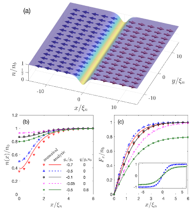
Figure 1: (a) Schematic of a transverse magnetic domain wall (along $y$-axis) in a system of background density $n_{b}$. The arrows represents the transverse magnetization vector $(F_{x},F_{y})$, and the background color shows the superfluid density. A comparison between analytical predictions (lines) and numerical results (symbols) for the (b) density and (c) $F_{x}$ spin density for various values of $g_{s}/g_{n}$ and $q$. The inset shows two complete profiles of $F_{x}$ at the exactly solvable point with $q=0$ and $q\neq 0$, respectively. Here $\xi_{n}=\hbar/\sqrt{Mg_{n}n_{b}}$ is the density healing length.

In this paper we present an analytic solution of a stable magnetic domain wall in a quasi-2D spin-1 ferromagnetic BEC, characterized by magnetization $\mathbf{F}$ having the typical profile of a dark soliton [Fig. 1(a)] : a $\pi$ phase (direction of $\mathbf{F}$) jump crossing the domain wall and $\mathbf{F}=\mathbf{0}$ at the centre, breaking the $\mathbb{Z}_{2}$ symmetry. In contrast to most domain walls/solitons in BECs, the magnetic domain wall is stable against the snake instability in two dimensions. This is verified by studying transverse standing waves on these domain walls, finding they oscillate without decay. Instead, the system has a linear dynamic instability driven by modes localized near the domain wall core that cause a growth of the perpendicular components of the magnetization. The resulting spin texture corresponds to a chain of spin vortex anti-vortex pairs along the domain wall. Real time dynamics in the presence of white noise shows that the magnetic domain wall survives. Exact solutions are obtained for a large spin-dependent interaction strength $g_{s}$ with and without magnetic fields. These exact solutions are distinct from two well-known solvable cases: the Manakov regime Manakov (1974) ($g_{s}=0$ in spin-1 BECs) and the magnetic soliton regime (constant number density) Qu et al. (2016). In the absence of magnetic fields, $\textrm{SO}(3)$ spin rotations relate a family of degenerate solutions, and we show that for particular rotations the underlying component wavefunction can map onto a range of solitons and domain walls proposed for binary condensates. Thus a distinct set of unrelated non-linear excitations are found to be contained within our solution, unified by its symmetries.

II Formalism for a spin-1 BEC

The Hamiltonian density of a quasi-2D spin-1 BEC foo (a) reads

$${\cal H}=\frac{\hbar^{2}\left|\nabla\psi\right|^{2}}{2M}+\frac{g_{n}}{2}|\psi^{{\dagger}}\psi|^{2}+\frac{g_{s}}{2}|\psi^{{\dagger}}\mathbf{S}\psi|^{2}+q\psi^{{\dagger}}S^{2}_{z}\psi,$$ (1)

where the three component wavefunction ${\psi}=(\psi_{+1},\psi_{0},\psi_{-1})^{T}$ describes the condensate amplitude in the $m=+1,0,-1$ sublevels, respectively. Here $M$ is the atomic mass, $g_{n}>0$ is the density interaction strength, $g_{s}$ is the spin-dependent interaction strength, $\mathbf{S}=(S_{x},S_{y},S_{z})$ with $S_{\nu=x,y,z}$ being the spin-1 matrices foo (b), and $q$ denotes the quadratic Zeeman energy. The spin-dependent interaction term allows for spin-mixing collisions in which two $m=0$ atoms collide and convert into $m=+1$ and $-1$ atoms, and the reverse process.

The dynamics of the field $\psi$ is given by the Gross-Pitaevskii equations (GPEs) $i\hbar\partial\psi/\partial t=\delta{\cal H}/\delta\psi^{{\dagger}}\equiv\cal{L}_{\rm{GP}}\psi$, which in component form is

$$\!\!\!\!i\hbar\frac{\partial\psi_{\pm 1}}{\partial t} =\left[H_{0}+g_{s}\left(n_{0}+n_{\pm 1}-n_{\mp 1}\right)+q\right]\psi_{\pm 1}+g_{s}\psi^{2}_{0}\psi^{*}_{\mp 1},$$ (2a)

$$\!\!\!\!i\hbar\frac{\partial\psi_{0}}{\partial t} =\left[H_{0}+g_{s}\left(n_{+1}+n_{-1}\right)\right]\psi_{0}+2g_{s}\psi^{*}_{0}\psi_{+1}\psi_{-1},$$ (2b)

where $H_{0}=-\hbar^{2}\nabla^{2}/2M+g_{n}n$, with $n=\sum_{m}n_{m}$ and $n_{m}=|\psi_{m}|^{2}$ being the total and component densities, respectively. Spin-1 BECs exhibit magnetic order, e.g., the magnetization $\mathbf{F}\equiv\psi^{{\dagger}}\mathbf{S}\psi$ mag is the order parameter of ferromagnetic phases $|\mathbf{F}|>0$ for $g_{s}<0$ (⁸⁷Rb or ⁷Li). In contrast anti-ferromagnetic phases with $g_{s}>0$ (²³Na) have $\mathbf{F}=0$. In the absence of magnetic fields, i.e. $q=0$, ${\cal H}$ is invariant under $\textrm{SO}(3)$ spin-rotations and the total magnetization $\int d^{2}\mathbf{r}\ \mathbf{F}$ is conserved.

III Dark soliton-like magnetic domain walls

For a uniform ferromagnetic system with total density $n_{b}$ and at $q=0$, the energy density ${\cal H}=g_{n}n^{2}_{b}/2+g_{s}|\mathbf{F}|^{2}/2$ is minimized for states with $|\mathbf{F}|=n_{b}$. The chemical potential is $\mu=(g_{n}+g_{s})n_{b}$. We search for a straight line domain wall connecting the two distinct magnetic ground states characterized by $\mathbf{F}=\pm n_{b}\hat{\mathbf{e}}$, where $\hat{\mathbf{e}}$ is a 3D unit vector along an arbitrary direction [see Fig. 1(a)]. For convenience, the domain wall is chosen parallel to the $y$-axis and the core is located at $x=0$. We find a solution of the general form

$$\mathbf{F}\simeq n(x)\tanh\left({x}/{\ell}\right)\hat{\mathbf{e}},$$ (3)

where $\ell=\hbar/\!\sqrt{4|g_{s}|Mn_{b}}$. This result is exact for a particular set of interaction parameters, and a good approximation in general as we discuss further below. This domain wall is of the Ising type, rather than the Bloch or Néel type, signified by $\mathbf{F}$ vanishing at the core and changing its sign across the core. The solution (3) has the characteristic profile of dark soliton and we refer to it as dark soliton-like magnetic domain wall (MDW). This domain wall is in magnetic order but not in the superfluid order, i.e. the superfluid density $n(x)$ does not vanish, but has a dip at the core to minimize the energy.

III.1 Exact solutions

When the width of the density dip coincides with $\ell$, occurring at $g_{s}=-g_{n}/2$ foo (c), Eq. (2) admits an exact solution

$$\mathbf{F}(x)=n_{b}\tanh\left(\frac{x}{2\ell}\right)\hat{\mathbf{e}},\quad n(x)=n_{b}\left[1-\frac{1}{2}\operatorname{sech}^{2}\left(\frac{x}{2\ell}\right)\right].$$ (4)

This system has a $\textrm{SO}(3)$ symmetry which relates a continuous family of degenerate MDW solutions connected by $\textrm{U}(1)$ gauge and spin ${\cal U}(\alpha,\beta,\tau)=e^{-i\alpha S_{z}}e^{-i\beta S_{y}}e^{-i\tau S_{z}}$ rotations, where $\{\alpha,\beta,\tau\}$ are the Euler angles. We illustrate three members of this family in Table 1: (i) For the case of an $F_{x}$ domain wall [i.e. $\hat{\mathbf{e}}=\hat{\mathbf{x}}$], the underlying wavefunctions can have two distinct vector soliton profiles, and the corresponding stationary GPE can be mapped onto that of a miscible binary BEC. (ii) A Sine-Gordon type soliton (SGS) of the phase difference $\theta_{d}\equiv\theta_{\pm 1}-\theta_{0}$, where $\psi_{m}=|\psi_{m}|e^{i\theta_{m}}$. A SGS has been predicted to exist in a coherently-coupled binary BEC, with dynamics mimicking processes in quantum chromodynamics Son and Stephanov (2002). Here the SGS can be produced by a spin rotation of the vector soliton in Table 1 and the nonlinear spin-mixing interaction provides the necessary couplings between the component phases, having the advantage that no external fields are required foo (d). (iii) For an $F_{z}$ domain wall, the corresponding wavefunction coincides with a (density) domain wall of an immiscible binary BEC Ao and Chui (1998).

($\alpha$, $\beta$, $\tau$)	type-I: 0;  type-II: ($\pi/2$, $-\pi/2$, $-\pi/2$)	($-\pi/2$, $-\pi/4$, $-\pi/2$)	($\pi/2$, $\pi/2$, $0$)
U(1)	type-I: 1;  type-II: $e^{i\pi/2}$	$e^{-i\pi/4}$	$e^{i3\pi/2}$
$\psi\big{|}_{g_{s}=-g_{n}/2}$	I: $\psi_{\pm 1}=\sqrt{n_{b}}/2\tanh\left(x/2\ell\right)$; $\psi_{0}=\sqrt{n_{b}/2}$	$\psi_{\pm 1}=\sqrt{n_{\pm 1}}e^{i\theta_{d}/2},\psi_{0}=\sqrt{n_{0}}e^{-i\theta_{d}/2}$	$\psi_{\pm 1}=\sqrt{n_{b}}/2\left[1\mp\tanh\left(x/2\ell\right)\right]$
	II: $\psi_{\pm 1}=\sqrt{n_{b}}/2,\psi_{0}=\sqrt{n_{b}/2}\tanh(x/2\ell)$	$\theta_{d}(x)=2\arctan e^{x/\ell}$, $2n_{\pm 1}=n_{0}=n/2$	$\psi_{0}=0$
$\mathbf{F}$	$F_{x}=n_{b}\tanh\left(x/2\ell\right)$	$F_{x}=n_{b}\tanh\left(x/2\ell\right)$	$F_{z}=-n_{b}\tanh\left(x/2\ell\right)$
GPE	$0=\left[H^{\prime}+2g_{n}n_{\pm 1}+(g_{n}+2g_{s})n_{0}\right]\psi_{\pm 1}$	$0=\frac{\hbar^{2}}{2M}\partial_{x}(n\partial_{x}\theta_{d})+g_{s}n^{2}\sin(2\theta_{d})$	$0=\left[H^{\prime}+(g_{n}+g_{s})n_{+1}+(g_{n}-g_{s})n_{-1}\right]\psi_{+1}$
	$0=\left[H^{\prime}+g_{n}n_{0}+2(g_{n}+2g_{s})n_{\pm 1}\right]\psi_{0\phantom{+}}$	$0=\frac{\hbar^{2}}{2M}\left[\frac{1}{2}(\partial_{x}\theta_{d})^{2}-\frac{2}{\sqrt{n}}\partial^{2}_{x}\sqrt{n}\right]$	$0=\left[H^{\prime}+(g_{n}+g_{s})n_{-1}+(g_{n}-g_{s})n_{+1}\right]\psi_{-1}$
	$H^{\prime}=-\frac{\hbar^{2}}{2M}\partial_{x}^{2}-\mu$	$\phantom{0=}+2[n(g_{n}+g_{s}\cos^{2}\theta_{d})-\mu]$
Related systems	Vector soliton of a three-component BEC and a miscible binary BEC	Sine-Gordon type soliton, also realized in a coherently-coupled binary BEC	Density domain wall of an immiscible binary BEC

Table 1: Component representation of the MDW after various spin rotations. Vector soliton sector: type-I vector soliton is chosen as a reference point. In this presentation, the reduced GPEs are related to a miscible binary system and becomes decoupled at $g_{s}=-g_{n}/2$, allowing the exact solution. SGS: $\theta_{d}$ satisfies the Sine-Gordon equation. Binary domain wall sector: the reduced GPEs describe an immiscible binary system and the corresponding exact solution coincides with a solution discussed in a different context Malomed et al. (1990).

In the context of binary BECs, the vector solitons, the SGS and the density domain wall are unrelated. In a spin-1 BEC, these distinct nonlinear excitations are unified by spin rotations of our MDW solution. With inadequate degrees of freedom and symmetries, such connection can not be made within the binary BEC foo (e); Stamper-Kurn and Ueda (2013). However it is important to note that the dynamics and stability properties of the MDW reveal the spin-1 nature and exhibit distinct behaviors from related excitations in binary systems (see below). A recent study on magnetic solitons in anti-ferromagnetic BECs has also explored the role of the rotational symmetry Chai et al. (2021).

III.2 Away from the exactly solvable point

Away from the exactly solvable point we develop a self-consistent asymptotic analysis of the stationary GPEs at $x\gg\ell$, combined with an account of the local core structure, and we find an accurate approximate form for the density

$$\frac{n(x)}{n_{b}}\simeq \frac{\cosh(x/\lambda\ell)}{a_{1}\cosh(x/\lambda\ell)+a_{1}^{2}b_{1}}+1-\frac{1}{a_{1}}, g_{s}<-\frac{g_{n}}{5}$$ (5a)

$$\frac{n(x)}{n_{b}}\simeq 1+\frac{4b_{1}\,g_{s}}{2(g_{n}+g_{s})\cosh^{2}(x/\ell)+g_{1}}, -\frac{g_{n}}{5}<g_{s}$$ (5b)

where $\lambda=\sqrt{-g_{s}/(g_{n}+g_{s})}$, $a_{1}=-(2g^{2}_{n}+2g_{n}g_{s}-g_{s}^{2})/(3g_{s}(g_{n}+g_{s}))$, $b_{1}=3(g_{n}+g_{s})/(2g_{n}+g_{s})$, and $g_{1}=2b_{1}(2g_{n}-5g_{s})/3$.

In the following we show the procedure to obtain Eqs. (5b). Specializing to the SGS (see Table 1) we work with the hydrodynamical variables $\{n,n_{d},\theta_{d},\theta_{s}\}$, where $n_{d}=2n_{\pm 1}-n_{0}$, $\theta_{s}=\theta_{\pm 1}+\theta_{0}$, $\theta_{+1}=\theta_{-1}$ and $n_{+1}=n_{-1}$. For a stationary state, the total number current $\mathbf{J}_{n}=\hbar^{2}/(2M)\left(n\bm{\nabla}\theta_{s}+n_{d}\bm{\nabla}\theta_{d}\right)$ should vanish. Apparently $\theta_{s}=0$ and $n_{d}=0$ solve $\mathbf{J}_{n}=0$, and for this case Eqs. (2) [or Eqs. (19)] reduce to

$$0 =\frac{\hbar^{2}}{2M}\partial_{x}(n\partial_{x}\theta_{d})+g_{s}n^{2}\sin(2\theta_{d}),$$ (6a)

$$\mu =\frac{\hbar^{2}}{4M}\left[\frac{(\partial_{x}\theta_{d})^{2}}{2}-\frac{2\partial^{2}_{x}\sqrt{n}}{\sqrt{n}}\right]+{g_{s}n}\cos^{2}\theta_{d}+g_{n}n.$$ (6b)

As shown in Table 1, at $g_{s}=-g_{n}/2$,

$$\theta_{d}(x)=2\arctan e^{x/\ell},$$ (7)

where $\ell=\hbar/\sqrt{4|g_{s}|Mn_{b}}$ as introduced earlier. Away from the exactly solvable point we assume that the expression of $\theta_{d}(x)$ in Eq. (7) remains a good approximation. In other words, $\mathbf{F}/n(x)$ is assumed to take the same form as at the exactly solvable point. The reason for this will become clear later.

Let us examine the asymptotic form of Eq. (6b) far away from the core $x=0$. Assuming that $g(x)\equiv[n(x)-n_{b}]/(4n_{b})$ decays slower than $(\partial_{x}\theta_{d})^{2}\sim e^{-2x/\ell}$ for large $x\gg\ell$ (there is no solution for $g(x)$ decaying faster than $e^{-2x/\ell}$), in the large $x$ limit, the dominant part of Eq. (6b) reads

$$\left(g_{n}+g_{s}\right)g(x)+\ell^{2}g_{s}g^{\prime\prime}(x)=0,$$ (8)

having a solution $g(x\gg\ell)\sim e^{-x/\ell_{d}}$, where $\ell_{d}=\lambda\ell$ is the effective density length scale. Combining the asymptotic behavior of $n(x)$ at large $x$ and $n(x)$ being an even function, it is natural to propose the ansatz (5a). The coefficients $a_{1}$ and $b_{1}$ are introduced to adjust the core structure and are determined by requiring that $n(x)$ satisfies Eqs. (6) to leading order as $x\rightarrow 0$. The working assumption to obtain Eq. (5a) is $\ell_{d}>\ell(\lambda>1/2)$, implying $g_{n}+5g_{s}<0$ which sets the parameter range for the solution in Eq. (5a) to be applicable. This regime includes the exactly solvable point, $g_{s}=-g_{n}/2$ with $\lambda=1$, where $\ell_{d}=\ell$, and a single length scale describes the spin and density character of the MDW [here (5a) reduces to Eq. (4)]. In this strong spin interaction regime (5a), the density variation near the core is important. The excitation breaks down at $g_{s}+g_{n}=0$ which is the parameter boundary of the ferromagnetic phaseStamper-Kurn and Ueda (2013); Kawaguchi and Ueda (2012).

In the opposite limit, where $|g_{s}/g_{n}|\ll 1$, the quantum pressure term $\sim\partial^{2}_{x}\sqrt{n}/\sqrt{n}$ becomes less important and can be neglected. Hence Eq. (6b) becomes an algebraic equation of $n(x)$ with solution given Eq. (5b). The parameters $b_{1}$ and $g_{1}$ are introduced to solve Eqs. (6) near the core $x=0$ to leading order. The crossover to the weak spin interaction regime (5b) occurs at $g_{n}+5g_{s}=0$ where $\lambda=1/2$, given by matching the density widths $\ell/2$ and $\ell_{d}$. For comparison we calculate numerical MDW results using a gradient flow method Lim and Bao (2008); Bao and Lim (2008). The analytic and numerical results in Figs. 1(b) and (c) show excellent agreement.

Let us now provide a self-consistent reasoning to explain why $\theta_{d}(x)$ in Eq. (7) serves a good approximation in the whole parameter range. First of all, it captures the main feature of the domain wall in the strongly interacting regime where the exact solution Eq. (7) is found. On the other hand, in the weak interaction limit ($|g_{s}/g_{n}|\ll 1$) the density $n$ can be approximated as a constant ($n\simeq n_{b}$) and the energy density becomes

$${\cal H}=-\frac{\hbar^{2}n}{8M}|\nabla\theta_{d}|^{2}+\frac{g_{n}}{2}n_{b}-\frac{1}{2}g_{s}n_{b}^{2}\cos^{2}\theta_{d}.$$ (9)

A local minimum of the energy density, determined by $\delta{\cal H}/\delta\theta_{d}=0$, leads to the elliptic sine-Gordon equation $\hbar^{2}/(2M)\nabla^{2}(2\theta_{d})+2n_{b}g_{s}\sin(2\theta_{d})=0$, having the solution $\theta_{d}=2\arctan e^{x/\ell}$.

Since the magnetization vanishes at the core, there is no spin current across the MDW. However, the nematic tensor current is nontrivial foo (f). The component number currents vary for different degenerate states. For example, with reference to the states in Table 1: the component currents are zero for the vector soliton, while for SGS there are internal currents near the core that behave analogously to Josephson currents Barone and Paterno (1982).

IV Finite magnetic fields

A magnetic field along the $z$-axis breaks the $\textrm{SO}(3)$ symmetry and the degeneracy of states presented in Table 1 is lifted. For $q>0$ the ground state magnetization prefers to be transverse, realizing an easy-plane ferromagnetic phase that possesses a remnant $\textrm{SO}(2)$ symmetry Stamper-Kurn and Ueda (2013); Kawaguchi and Ueda (2012). Here the SGS and the binary density domain wall are no longer stationary solutions. The type-I vector soliton is energetically favored, and exists, with some modifications, in the whole easy-plane phase ($0<q<2|g_{s}|n_{b}$). At $g_{s}=-g_{n}/2$, the exact solution is

$$\mathbf{F} = n_{b}\sqrt{1-\tilde{q}^{2}}\tanh\left(\frac{x}{2\ell_{q}}\right)\hat{\mathbf{e}}_{\rho},$$ (10)

$$n(x) = n_{b}\left[1-\frac{1-\tilde{q}}{2}\operatorname{sech}^{2}\left(\frac{x}{2\ell_{q}}\right)\right],$$ (11)

where $\tilde{q}=-q/2g_{s}n_{b}$, $\ell_{q}=\!\ell/\sqrt{1-\tilde{q}}$ and $\hat{\mathbf{e}}_{\rho}$ is a unit vector in the $xy$-plane. The corresponding wavefunction reads $\psi_{\pm 1}=\sqrt{n_{b}(1-\tilde{q})/4}\tanh\left(x/2\ell_{d}\right)$, and $\psi_{0}=\sqrt{n_{b}(1+\tilde{q})/2}$. An example of a $q\neq 0$ result ($\hat{\mathbf{e}}_{\rho}=\hat{\mathbf{x}}$) is shown in Fig. 1.

V Standing waves

A conspicuous feature of the 2D dynamics of the MDW is that it is stable against transverse deformations, strikingly different from other domain walls/solitons Kuznetsov and Turitsyn (1988); Muryshev et al. (1999); Anderson et al. (2001); Son and Stephanov (2002); Ihara and Kasamatsu (2019); Gallemí et al. (2019); Qu et al. (2016); Farolfi et al. (2020); Chai et al. (2020); Kang et al. (2019) which decay unavoidably via snake instability. We consider easy-plane domains with $\mathbf{F}$ along the $x$-axis and two fundamental static MDW geometries in the $x$-$y$ plane for $q=0$: closed circle and open straight line with endpoints attached on the boundaries foo (g) (see Fig. 2). We excite standing waves on these static MDWs by deforming them transversely. The subsequent time evolution shown in Figs. 2(a)-(c) is periodic and resembles harmonic modes vibrations foo (h). Our simulations Symes et al. (2016) also show that the standing waves persist without decay, combined with internal spin-exchange dynamics between components of the wavefunction (see Fig. 6 in Appendix B). During the time evolution $F_{y}$ and $F_{z}$ remain zero, the magnetization conservation manifests itself as a geometrical constraint of the domain wall motion: the area enclosed by the domain wall remains unchanged. There is no spin current crossing the MDW. The enclosed regions form magnetic bubbles, inside which the magnetization $F_{x}$ has the opposite orientation from the outer one and such feature remains in the presence of noise (see Fig. 2 and Fig. 3). Consequently, propagating open MDWs and expanding/shrinking closed MDWs are prohibited, becoming possible when applying magnetic fields along the $z$-axis.

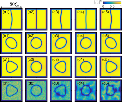
Figure 2: One period of evolution for standing wave deformations of a MDW confined by hard wall potentials in a square domain $x,y\in[-L,L]$ with $L=40\xi_{n}$. The equilibrium configurations are shown in the second and forth columns. (a1)-(a5) A standing wave on an open MDW with free end-points attached on the hard wall boundaries; the initial configuration (MDW core location) is $x=A\cos(\pi y/L)$, $y\in[-L,L]$ with $L=40\xi_{n}$ and $A=2.5\xi_{n}$. (b1)-(b5), (c1)-(c5) Standing waves on a closed MDW. The initial configurations are determined by $R_{0}-\sqrt{x^{2}+y^{2}}+A\sin[s\arctan(y/x)]=0$ where $R_{0}=L/2$, $s=2$ (dipole mode) for (b1) and $s=3$ (triple mode) for (c1). Oscillation periods $T$ are: (a) $T\simeq 620t_{0}$; (b) $T\simeq 620t_{0}$; (c) $T\simeq 300t_{0}$, where $t_{0}=\hbar/g_{n}n_{b}$ and $g_{s}/g_{n}=-0.1$. (d1)-(d5) Results with white noise added to the initial condition of (c1), causing a $\!\sim\!1$% increase in particle number. Such stability also stands for the open domain walls. Note that for (a) (b) and (c) $|F_{x}|=|\mathbf{F}|$.

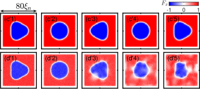
Figure 3: The transverse magnetization $F_{x}$ during the time evolution. $(\text{c}^{\prime}1)$-$(\text{c}^{\prime}5)$ and $(\text{d}^{\prime}1)$-$(\text{d}^{\prime}5)$ correspond to Fig. 2(c1)-(c5) and (d1)-(d5), respectively.

VI Dynamical instability

Here we systematically study the stability of the MDW by means of Bogoliubov-de Gennes equations (BdGs). Let us consider a straight infinitely long MDW along the $y$-axis located in the middle of a slab of width $L_{s}\gg\ell$. Denoting the stationary MDW as $\psi_{s}$, we consider a perturbation $\delta\psi=u(\mathbf{r})e^{-i\omega t}+v^{*}(\mathbf{r})e^{i\omega^{*}t}$. Linearizing about $\psi=\psi_{s}+\delta\psi$ in Eq. (2) yields the BdG equations

$$\hbar\omega\left({\begin{array}[]{cc}u\\ v\\ \end{array}}\right)=\left({\begin{array}[]{cc}{\cal L}_{\rm GP}+X-\mu&\Delta\\ -\Delta^{*}&-({\cal L}_{\rm GP}+X-\mu)^{*}\\ \end{array}}\right)\left({\begin{array}[]{cc}u\\ v\\ \end{array}}\right),$$ (18)

where the stationary wavefunction satisfies ${\cal L}_{\rm GP}\psi_{s}=\mu\psi_{s}$, $X=g_{s}\sum_{\nu}S_{\nu}\psi_{s}\psi_{s}^{\dagger}S_{\nu}+g_{n}\psi_{s}\psi^{\dagger}_{s}$, $\Delta=g_{n}\psi_{s}\psi^{T}_{s}+g_{s}\sum_{\nu}(S_{\nu}\psi_{s})(S_{\nu}\psi_{s})^{T}$ and $\mu=(g_{n}+g_{s})n_{b}+q/2$.

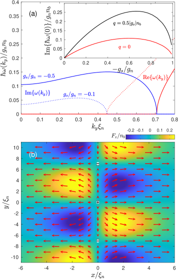
Figure 4: Unstable spin-twist modes. (a) Spectrum of the unstable modes for $q=0$ and two values of $g_{s}/g_{n}$. For $g_{s}/g_{n}=-1/2$ the bifurcation point ($\omega=0$) occurs exactly at $k_{y}\xi_{n}=1/\sqrt{2}$. Insets shows the magnitude of the long wavelength instability as $g_{s}/g_{n}$ varies. (b) The spin-texture created by the unstable mode foo (i) at $k_{y}\xi_{n}\simeq 0.445$ where the maximum imaginary frequency is reached for $q=0$ and $g_{s}/g_{n}=-1/2$. White circles with $+$ and $-$ indicating positive and negative circulation spin-vortices, respectively. The red arrows and the background color represent transverse magnetization field $(F_{x},F_{y})$ and longitudinal magnetization $F_{z}$, respectively.

The translational symmetry along $y$ allows us to parameterize the perturbations with the wave-vector $k_{y}$ as $u(\mathbf{r})=u(x)e^{ik_{y}y}$ and $v(\mathbf{r})=v(x)e^{ik_{y}y}$. We numerically solve Eq. (18) with Neumann boundary conditions at $x$-axis boundaries foo (j), and find two modes with an imaginary energy [Fig. 4(a)], marking a dynamical instability in the system (a mode that grows exponentially with time).

Different from the snake instability Muryshev et al. (1999), the imaginary part of the excitation energy $\rm Im(\omega)$ does not vanish as $k_{y}\to 0$, but instead approaches a finite value [Fig. 4(a)], implying that this instability also exists in 1D. $F_{x}$ is unchanged as the unstable mode grows, however it causes the unmagnetized core of the MDW to develop a $F_{y}$-texture of wavelength $\pi/k_{y}$. This corresponds to the formation of a chain of “magnetic vortex” cores foo (k) at the nodes of this texture [Fig. 4(b)].

The $k_{y}$ range of unstable modes and the magnitude of the imaginary energy is largest at intermediate values of $g_{s}/g_{n}$, and increases with increasing $q$ [see inset to Fig. 4(a)]. Based on the magnetic texture created by the unstable mode, we refer to it as spin-twist instability. In dynamics the growth of this instability leads to spin waves of $F_{y}$ and $F_{z}$ while the topological structure of the MDW in $F_{x}$ remains unchanged, consistent with the noisy dynamics observed in Fig. 2(d). Note that this characteristic feature does not rely on the conservation law of magnetization, and holds in the presence of magnetic fields ($q>0$). The growth of $F_{y}$ and $F_{z}$ could be stabilizing the domain wall by absorbing the perturbations, in analogy to a buffering effect.

VII Conclusion and outlook

We found a novel magnetic domain wall in a quasi-2D ferromagnetic spin-1 BEC that is stable against the snake instability and white noise. Along with the exact solutions, an accurate analytic solution applicable to the whole ferromagnetic phase has also been developed. Through the underlying symmetries of the spin-1 system, we have shown that various distinct nonlinear structures such as the Sine-Gordon soliton, vector solitons and an immiscible binary density domain wall occurring in unrelated binary systems are unified into the magnetic domain wall. Our findings open a new possibility to study rich 2D dynamics of domain wall solitons, could be important for determining the universality class of the ferromagnetic phase transition of 2D spin-1 BECs at finite temperature James and Lamacraft (2011); Kobayashi (2019), coarsening dynamics involving both spin order and superfluid order Bourges and Blakie (2017); Prüfer et al. (2018) and dynamics of stretched polar-core vortices Williamson and Blakie (2016b); Turner (2009).

It will be feasible to observe magnetic domain walls in current experiments with ferromagnetic spinor BECs. The necessary techniques for manipulating the spin degrees of freedom of a spin-1 BEC Chai et al. (2020), and for non-destructively measuring its spin dynamics Higbie et al. (2005) have already been demonstrated. Coupled with a planar or flat-bottom optical trap (e.g. Chomaz et al. (2015); Gauthier et al. (2016)) opens the possibility for investigating of domain wall dynamics. Most work with ferromagnetic spin-1 BECs to date has been conducted with ⁸⁷Rb which has $-g_{s}/g_{n}\sim 10^{-2}$ and is in the weakly spin-interacting regime. However, recently a ⁷Li spin-1 BEC has been prepared with $-g_{s}/g_{n}\sim 0.5$ Huh et al. (2020), thus in the strong spin interacting regime close to the exactly solvable point.

VIII Acknowledgment

We thanks M. Antonio, T. Luke, L. A. Williamson, Russell Bisset and Danny Baillie for useful discussions. X.Y. acknowledges the support from NSAF through grant number U1930403. P.B.B acknowledges support from the Marsden Fund of the Royal Society of New Zealand.

Appendix A Spin-1 Gross-Pitaevskii equations in hydrodynamical variables

In terms of the hydrodynamical variables $\{n,n_{d},\theta_{d},\theta_{s}\}$, the stationary GPE for $q=0$ becomes

$$0 =-\frac{\hbar^{2}}{2M}\nabla\cdot(n\nabla\theta_{s}+n_{d}\nabla\theta_{d}),$$ (19a)

$$0 =\frac{\hbar^{2}}{2M}\nabla\cdot(n\nabla\theta_{d}+n_{d}\nabla\theta_{s})+g_{s}(n^{2}-n^{2}_{d})\sin(2\theta_{d}),$$ (19b)

$$0 =-\frac{\hbar^{2}}{2M}\left[\frac{1}{\sqrt{n+n_{d}}}\nabla^{2}\sqrt{n+n_{d}}+\frac{1}{\sqrt{n-n_{d}}}\nabla^{2}\sqrt{n-n_{d}}-\frac{1}{2}(|\nabla\theta_{s}|^{2}+|\nabla\theta_{d}|^{2})\right]+g_{s}n\cos(2\theta_{d})+(g_{s}+2g_{n})n-2\mu,$$ (19c)

$$0 =\frac{\hbar^{2}}{2M}\left[\frac{1}{\sqrt{n+n_{d}}}\nabla^{2}\sqrt{n+n_{d}}-\frac{1}{\sqrt{n-n_{d}}}\nabla^{2}\sqrt{n-n_{d}}-\nabla\alpha\cdot\nabla\beta\right]+g_{s}n_{d}\cos(2\beta)+g_{s}n_{d},$$ (19d)

where $n_{d}=2n_{\pm 1}-n_{0}$, $\theta_{s}=\theta_{\pm 1}+\theta_{0}$, $\theta_{d}=\theta_{\pm 1}-\theta_{0}$, $n=n_{+}+n_{-}+n_{0}$, $\mu=(g_{n}+g_{s})n_{b}$ is the chemical potential and $n_{b}$ is the ground state total number density. Here we assume that $\theta_{+1}=\theta_{-1}$ and $n_{+1}=n_{-1}$.

Appendix B Real time evolution

Here we present further evidence of the stability. Figure 3 shows that the topological nature of the MDW, i.e. the $\pi$ phase jump across the core, is well preserved during the domain wall motion. This can be also seen in Fig. 5(a) which shows the profile of the transverse magnetization $F_{x}(x,y=0)$ at different times.

In our simulations, the box potential takes the following form

$$V(x,y)=V_{0}\left\{2-\tanh\left[\left(\frac{L}{c}-|x|\right)b\right]-\tanh\left[\left(\frac{L}{c}-|y|\right)b\right]\right\},$$ (20)

where $x,y\in[-L,L]$, $L$ is the box size, $V_{0}\gg\mu$ is the hight of the potential barrier, $b\sim\xi^{-1}_{n}$ is the width and $c$ should be chosen slightly greater than one.

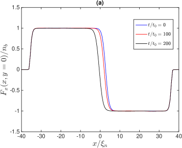
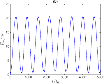
Figure 5: (a) shows the spin-density cross section $F_{x}(x,y=0)$ of the open MDW shown in Fig. 2(a) at different times. The soliton-like profile of the magnetization is preserved during the motion. (b) shows the periodic behavior of the overlap function for the open domain wall configuration [Fig. 2(a)], demonstrating that the standing wave on the MDW persists without decay over long time periods.

The standing wave excitation on the MDW can last a long time without decay. In order to quantify this property, we introduce an overlap function

$$O(t)\equiv\left(\int d^{2}\mathbf{r}\left|F_{x}(\mathbf{r},t)-F_{x}(\mathbf{r},0)\right|^{2}\right)^{1/2}$$ (21)

that measures the overlap of transverse magnetization profile at time $t$ with its initial profile. Figure 5(b) shows the periodic behavior of $O(t)$ for the open domain wall [Fig.2(a)], revealing that the standing wave on the MDW persists without decay.

It is worthwhile to mention that along with the domain wall oscillation, components of the wavefunction exhibit spin-exchange dynamics [Fig.6].

Figure 6: Spin-exchange dynamics during the MDW oscillation shown in Fig. 2(a1)-(a5). (e1)-(e5), (f1)-f(5) show dynamics of component densities $2n_{\pm 1}$ and $n_{0}$, respectively.

References

- Bunkov and Godfrin (2012) Yuriy M Bunkov and Henri Godfrin, Topological defects and the non-equilibrium dynamics of symmetry breaking phase transitions, Vol. 549 (Springer Science & Business Media, 2012).
- Manton and Sutcliffe (2004) Nicholas Manton and Paul Sutcliffe, Topological solitons (Cambridge University Press, 2004).
- Eto et al. (2014) Minoru Eto, Yuji Hirono, Muneto Nitta, and Shigehiro Yasui, “Vortices and other topological solitons in dense quark matter,” Progress of Theoretical and Experimental Physics 2014 (2014).
- Vilenkin and Shellard (2000) Alexander Vilenkin and E Paul S Shellard, Cosmic strings and other topological defects (Cambridge University Press, 2000).
- Kuznetsov and Turitsyn (1988) EA Kuznetsov and SK Turitsyn, “Instability and collapse of solitons in media with a defocusing nonlinearity,” Zh. Eksp. Teor. Fiz 94, 129 (1988).
- Muryshev et al. (1999) A. E. Muryshev, H. B. van Linden van den Heuvell, and G. V. Shlyapnikov, “Stability of standing matter waves in a trap,” Phys. Rev. A 60, R2665–R2668 (1999).
- Anderson et al. (2001) B. P. Anderson, P. C. Haljan, C. A. Regal, D. L. Feder, L. A. Collins, C. W. Clark, and E. A. Cornell, “Watching dark solitons decay into vortex rings in a bose-einstein condensate,” Phys. Rev. Lett. 86, 2926–2929 (2001).
- Huang et al. (2003) Guoxiang Huang, Valeri A. Makarov, and Manuel G. Velarde, “Two-dimensional solitons in bose-einstein condensates with a disk-shaped trap,” Phys. Rev. A 67, 023604 (2003).
- Son and Stephanov (2002) D. T. Son and M. A. Stephanov, “Domain walls of relative phase in two-component bose-einstein condensates,” Phys. Rev. A 65, 063621 (2002).
- Ihara and Kasamatsu (2019) Kousuke Ihara and Kenichi Kasamatsu, “Transverse instability and disintegration of a domain wall of a relative phase in coherently coupled two-component bose-einstein condensates,” Phys. Rev. A 100, 013630 (2019).
- Gallemí et al. (2019) A. Gallemí, L. P. Pitaevskii, S. Stringari, and A. Recati, “Decay of the relative phase domain wall into confined vortex pairs: The case of a coherently coupled bosonic mixture,” Phys. Rev. A 100, 023607 (2019).
- Qu et al. (2016) Chunlei Qu, Lev P. Pitaevskii, and Sandro Stringari, “Magnetic solitons in a binary bose-einstein condensate,” Phys. Rev. Lett. 116, 160402 (2016).
- Farolfi et al. (2020) A. Farolfi, D. Trypogeorgos, C. Mordini, G. Lamporesi, and G. Ferrari, “Observation of magnetic solitons in two-component bose-einstein condensates,” Phys. Rev. Lett. 125, 030401 (2020).
- Chai et al. (2020) X. Chai, D. Lao, Kazuya Fujimoto, Ryusuke Hamazaki, Masahito Ueda, and C. Raman, “Magnetic solitons in a spin-1 bose-einstein condensate,” Phys. Rev. Lett. 125, 030402 (2020).
- Kang et al. (2019) Seji Kang, Sang Won Seo, Hiromitsu Takeuchi, and Y. Shin, “Observation of wall-vortex composite defects in a spinor bose-einstein condensate,” Phys. Rev. Lett. 122, 095301 (2019).
- Ho (1998) Tin-Lun Ho, “Spinor bose condensates in optical traps,” Phys. Rev. Lett. 81, 742–745 (1998).
- Ohmi and Machida (1998) Tetsuo Ohmi and Kazushige Machida, “Bose-einstein condensation with internal degrees of freedom in alkali atom gases,” Journal of the Physical Society of Japan 67, 1822–1825 (1998).
- Sadler et al. (2006) L. E. Sadler, J. M. Higbie, S. R. Leslie, M. Vengalattore, and D. M. Stamper-Kurn, “Spontaneous symmetry breaking in a quenched ferromagnetic spinor bose–einstein condensate,” Nature 443, 312 EP – (2006).
- Stamper-Kurn and Ueda (2013) Dan M. Stamper-Kurn and Masahito Ueda, “Spinor bose gases: Symmetries, magnetism, and quantum dynamics,” Rev. Mod. Phys. 85, 1191–1244 (2013).
- Kawaguchi and Ueda (2012) Yuki Kawaguchi and Masahito Ueda, “Spinor bose–einstein condensates,” Physics Reports 520, 253 – 381 (2012), spinor Bose–Einstein condensates.
- Zhang et al. (2005) Wenxian Zhang, D. L. Zhou, M.-S. Chang, M. S. Chapman, and L. You, “Dynamical instability and domain formation in a spin-1 bose-einstein condensate,” Phys. Rev. Lett. 95, 180403 (2005).
- Higbie et al. (2005) J. M. Higbie, L. E. Sadler, S. Inouye, A. P. Chikkatur, S. R. Leslie, K. L. Moore, V. Savalli, and D. M. Stamper-Kurn, “Direct nondestructive imaging of magnetization in a spin-1 bose-einstein gas,” Phys. Rev. Lett. 95, 050401 (2005).
- Saito and Ueda (2005) Hiroki Saito and Masahito Ueda, “Spontaneous magnetization and structure formation in a spin-1 ferromagnetic bose-einstein condensate,” Phys. Rev. A 72, 023610 (2005).
- Saito et al. (2007) Hiroki Saito, Yuki Kawaguchi, and Masahito Ueda, “Topological defect formation in a quenched ferromagnetic bose-einstein condensates,” Phys. Rev. A 75, 013621 (2007).
- Zhang et al. (2007) Wenxian Zhang, Ö. E. Müstecaplıoğlu, and L. You, “Solitons in a trapped spin-1 atomic condensate,” Phys. Rev. A 75, 043601 (2007).
- Vengalattore et al. (2008) M. Vengalattore, S. R. Leslie, J. Guzman, and D. M. Stamper-Kurn, “Spontaneously modulated spin textures in a dipolar spinor bose-einstein condensate,” Phys. Rev. Lett. 100, 170403 (2008).
- Kawaguchi et al. (2010) Yuki Kawaguchi, Hiroki Saito, Kazue Kudo, and Masahito Ueda, “Spontaneous magnetic ordering in a ferromagnetic spinor dipolar bose-einstein condensate,” Phys. Rev. A 82, 043627 (2010).
- Williamson and Blakie (2016a) Lewis A. Williamson and P. B. Blakie, “Universal coarsening dynamics of a quenched ferromagnetic spin-1 condensate,” Phys. Rev. Lett. 116, 025301 (2016a).
- Prüfer et al. (2018) Maximilian Prüfer, Philipp Kunkel, Helmut Strobel, Stefan Lannig, Daniel Linnemann, Christian-Marcel Schmied, Jürgen Berges, Thomas Gasenzer, and Markus K. Oberthaler, “Observation of universal dynamics in a spinor Bose gas far from equilibrium,” Nature 563, 217–220 (2018).
- Nistazakis et al. (2008) H. E. Nistazakis, D. J. Frantzeskakis, P. G. Kevrekidis, B. A. Malomed, and R. Carretero-González, “Bright-dark soliton complexes in spinor bose-einstein condensates,” Phys. Rev. A 77, 033612 (2008).
- Busch and Anglin (2001) Th. Busch and J. R. Anglin, “Dark-bright solitons in inhomogeneous bose-einstein condensates,” Phys. Rev. Lett. 87, 010401 (2001).
- Bersano et al. (2018) T. M. Bersano, V. Gokhroo, M. A. Khamehchi, J. D’Ambroise, D. J. Frantzeskakis, P. Engels, and P. G. Kevrekidis, “Three-component soliton states in spinor bose-einstein condensates,” Phys. Rev. Lett. 120, 063202 (2018).
- Manakov (1974) Sergei V Manakov, “On the theory of two-dimensional stationary self-focusing of electromagnetic waves,” Soviet Physics-JETP 38, 248–253 (1974).
- foo (a) The size of the system in -direction is much smaller than the spin healing length .
-
foo (b)
Generators of the rotational
group :
.(31) - (36) ; ; .
- foo (c) In terms of scattering length, the exactly solvable point corresponds to , where is the s-wave scattering length in the total spin channel. Here we used the following relation and Ho (1998) .
- foo (d) In BEC experiments, the drawback of introducing Rabi-coupling (magnetic noise) sometimes can be problematic Trypogeorgos et al. (2018); Farolfi et al. (2019).
- Ao and Chui (1998) P. Ao and S. T. Chui, “Binary bose-einstein condensate mixtures in weakly and strongly segregated phases,” Phys. Rev. A 58, 4836–4840 (1998).
- Malomed et al. (1990) Boris A. Malomed, Alexander A. Nepomnyashchy, and Michael I. Tribelsky, “Domain boundaries in convection patterns,” Phys. Rev. A 42, 7244–7263 (1990).
- foo (e) Only in the Manakov limit, the two-component BEC possesses symmetry .
- Chai et al. (2021) Xiao Chai, Di Lao, Kazuya Fujimoto, and Chandra Raman, “Magnetic soliton: From two to three components with so(3) symmetry,” Phys. Rev. Research 3, L012003 (2021).
- Lim and Bao (2008) Fong Yin Lim and Weizhu Bao, “Numerical methods for computing the ground state of spin-1 bose-einstein condensates in a uniform magnetic field,” Phys. Rev. E 78, 066704 (2008).
- Bao and Lim (2008) Weizhu Bao and Fong Yin Lim, “Computing ground states of spin-1 bose–einstein condensates by the normalized gradient flow,” SIAM Journal on Scientific Computing 30, 1925–1948 (2008).
- foo (f) The details will be discussed elsewhere.
- Barone and Paterno (1982) Antonio Barone and Gianfranco Paterno, Physics and applications of the Josephson effect (Wiley, 1982).
- foo (g) Configurations with free ends are unstable .
- foo (h) For large deformations of the magnetic domain wall from its equilibrium position the motion is periodic but is not harmonic .
- Symes et al. (2016) L. M. Symes, R. I. McLachlan, and P. B. Blakie, “Efficient and accurate methods for solving the time-dependent spin-1 Gross-Pitaevskii equation,” Phys. Rev. E 93, 053309 (2016).
- foo (i) The BdG equation is , where is the BdG operator. The symmetry , with the Pauli matrix, ensures that is an eigenstate with eigenvalue . For the unstable modes, =0, hence . Then any linear combination of and is an eigenstate of . Here the unstable modes are chosen to be real, in which case the two unstable modes are identical.
- foo (j) The unstable modes must be localized in space and are insensitive to boundary conditions as long as .
- foo (k) In 2D vector fields with three components, winding number is not well defined and hence the terminology vortex is quoted.
- James and Lamacraft (2011) A. J. A. James and A. Lamacraft, “Phase diagram of two-dimensional polar condensates in a magnetic field,” Phys. Rev. Lett. 106, 140402 (2011).
- Kobayashi (2019) Michikazu Kobayashi, “Berezinskii–kosterlitz–thouless transition of spin-1 spinor bose gases in the presence of the quadratic zeeman effect,” Journal of the Physical Society of Japan 88, 094001 (2019).
- Bourges and Blakie (2017) Andréane Bourges and P. B. Blakie, “Different growth rates for spin and superfluid order in a quenched spinor condensate,” Phys. Rev. A 95, 023616 (2017).
- Williamson and Blakie (2016b) Lewis A. Williamson and P. B. Blakie, “Dynamics of polar-core spin vortices in a ferromagnetic spin-1 bose-einstein condensate,” Phys. Rev. A 94, 063615 (2016b).
- Turner (2009) Ari M. Turner, “Mass of a spin vortex in a bose-einstein condensate,” Phys. Rev. Lett. 103, 080603 (2009).
- Chomaz et al. (2015) Lauriane Chomaz, Laura Corman, Tom Bienaimé, Rémi Desbuquois, Christof Weitenberg, Sylvain Nascimbène, Jérôme Beugnon, and Jean Dalibard, “Emergence of coherence via transverse condensation in a uniform quasi-two-dimensional bose gas,” Nature communications 6 (2015).
- Gauthier et al. (2016) G. Gauthier, I. Lenton, N. McKay Parry, M. Baker, M. J. Davis, H. Rubinsztein-Dunlop, and T. W. Neely, “Direct imaging of a digital-micromirror device for configurable microscopic optical potentials,” Optica 3, 1136–1143 (2016).
- Huh et al. (2020) SeungJung Huh, Kyungtae Kim, Kiryang Kwon, and Jae-yoon Choi, “Observation of a strongly ferromagnetic spinor bose-einstein condensate,” Phys. Rev. Research 2, 033471 (2020).
- Trypogeorgos et al. (2018) D. Trypogeorgos, A. Valdés-Curiel, N. Lundblad, and I. B. Spielman, “Synthetic clock transitions via continuous dynamical decoupling,” Phys. Rev. A 97, 013407 (2018).
- Farolfi et al. (2019) A. Farolfi, D. Trypogeorgos, G. Colzi, E. Fava, G. Lamporesi, and G. Ferrari, “Design and characterization of a compact magnetic shield for ultracold atomic gas experiments,” Review of Scientific Instruments 90, 115114 (2019).