Lukash plane waves, revisited

Abstract

The Lukash metric is a homogeneous gravitational wave which at late times approximates the behaviour of a generic class of spatially homogenous cosmological models with monotonically decreasing energy density. The transcription from Brinkmann to Baldwin-Jeffery-Rosen (BJR) to Bianchi coordinates is presented and the relation to a Sturm-Liouville equation is explained. The 6-parameter isometry group is derived. In the Bianchi VII range of parameters we have two BJR transciptions. However using either of them induces a mere relabeling of the geodesics and isometries. Following pioneering work of Siklos, we provide a self-contained account of the geometry and global structure of the spacetime. The latter contains a Killing horizon to the future of which the spacetime resembles an anisotropic version of the Milne cosmology and to the past of which it resemble the Rindler wedge.

I Introduction

The standard approach to cosmology is to assume the Cosmological Principle which says that the Universe and its matter content are spatially homogeneous and isotropic ($SO(3)$ invariant) Hawking:1973uf ; Ehlers ; exactsol . This leads, locally at least, to the Friedmann-Lemaître-Robertson-Walker (FLRW) metric

$$ds^{2}=-dt^{2}+a^{2}(t)\,d\Omega^{2}_{K}\,,$$ (I.1)

where $d\Omega^{2}_{K}$ is the metric of constant curvature $K$ on

• 3-sphere      $\mathbb{S}^{3}=SO(4)/SO(3)$    if  $K=+1$ ,

• Euclidean space  $\mathbb{E}^{3}=E(3)/SO(3)$       if   $K=0$ ,

• hyperbolic space $\mathbb{H}^{3}=SO(3,1)/SO(3)$ if  $K=-1$ .

For general $a(t)$ the continuous isometries above, which act on the hypersurfaces of constant cosmic time $t$, are maximal. However if $a(t)=e^{Ht}$ and $K=0$ where $H=\sqrt{\frac{3}{\Lambda}}$, or if $K=-1$ and $a(t)=\frac{1}{H}\sinh(Ht)$, for example, then, despite appearances, the continuous isometries are much larger: $SO(4,1)$.

Typically the metric is singular at times when $a(t)=0$. The singularity is fictitious because the FLRW coordinates break down at $t=-\infty$ or $t=0$, respectively. The full spacetime accessible by past-directed timelike geodesics of finite propertime is de Sitter spacetime $SO(4,1)/SO(3,1)$ which is homogeneous Hawking:1973uf .

An even more striking example is obtained by setting $K=-1$ and take the limit $H\downarrow 0$. Then we find that $a(t)=t$, which is the Milne metric and is in fact flat. The FLRW coordinates cover only the interior of the future light cone of a point in Minkowski spacetime $E(4,1)/SO(3,1)$. Evidently past-directed time-like geodesics can leave the interior of the light cone in finite propertime. It is also clear that the same phenomenon occurs when $H\neq 0$.

A natural question to ask is whether such a behavior persists in the case of more general anisotropic cosmological models, i.e., those admitting a three-dimensional Bianchi-type subgroup $G_{3}$ of continuous isometries acting on spacelike hypersurfaces but for which there is no $SO(3)$ subgroup fixing points on those hypersurfaces.

The aim of the present paper is to explore a class of Ricci-flat solutions of the Einstein equations which exhibit a structure which is very similar to the Milne case : these are the Lukash solutions Lukash ; Lukash76 ; Lukash76 ; exactsol , which are of Bianchi type $VII_{h}$. This case is generic among Bianchi type groups, because it depends upon a dimensionless parameter $h$. The full isometry group is six-dimensional and admits a four dimensional subgroup which acts transitively on the complete spacetime.

Henceforth we restrict our attention at the $VII_{h}$ case. Other possibilities will be studied elsewhere.

Two Ricci-flat pp-waves are known to admit a six dimensional, multiply transitive isometry group Ehlers ; exactsol ; Sippel . They are : the “anti-Mach metric” OS which is a circularly polarised periodic (CPP) plane wave exactsol , and the Lukash plane wave Lukash ; Lukash74 ; Lukash76 .

CPP is a non-singular continuous gravitational wave OS ; exactsol ; Sippel ; CPP . Historically, it provided a powerful argument for the physical existence in Einstein’s theory of gravitational waves in the complete absence of material sources or localised patches of curvature, since the metric is spacetime-homogeneous, i.e., invariant under the action of a four-dimensional simply-transitive group of symmetries.

The metric of the Lukash wave (to which this paper is devoted) may be cast in Brinkmann coordinates,

$$ds^{2}=2dUdV+d{{\bf X}}^{2}+K(U,{\bf X})\,dU^{2}\,$$ (I.2)

with profile

$$K=-2\mathrm{Re}\bigl{(}C\zeta^{2}U^{2(i\kappa-1)}\bigr{)}\,$$ (I.3)

where $\zeta=({X^{1}}+i{X^{2}})/\sqrt{2}$ Siklos91 . Physically, $C$ represents the strength (amplitude) of the wave and $\kappa$ represents the polarisation. Although both could be real and $\kappa$ could even be complex, we shall only consider $C$ and $\kappa$ both positive.

Brinkman coordinates are well-defined for all $V,{\bf X}$ and $U>0$, but they break down at $U=0$. The nature of the singularity at $U=0$ was the subject of a number of investigations Siklos81 ; Siklos2 ; Siklos3 ; Siklos91 subsequent to Collins:1972tf ; Collins:1973lda ; Lukash ; Lukash74 ; Lukash76 and motivated in part by EllisKing1 .

Following Siklos91 the Bianchi VII group structure requires that the parameters satisfy Siklos91 ,

$$\text{\small either}\quad 0\leq C<\kappa\quad\text{\small or}\quad\kappa=C\,>1/2\,$$ (I.4)

we shall refer to as the Bianchi VII range.

The Lukash solutions, which contain the Milne metric as a special case, have attracted considerable attention in the past because of their cosmological applications. They have been shown to approximate at late times a wide class of spatially homogeneous (or cohomogeneity one) cosmological models with vanishing or negligible cosmological constant, in which the matter density also becomes negligible at late times Collins:1972tf ; Collins:1973lda ; EllisKing1 ; Barrow86 ; Barrow:2004gk ; Fliche ; Fliche2 ; Fliche3 .

A striking result of Collins:1972tf ; Collins:1973lda is that they do not isotropise, i.e., they do not approximate the Milne metric at late times. In fact they are stable at late times Barrow86 ; Barrow:2004gk ; Wainwright:1998ms ; Hsu . Thus, contrarily to what had been believed previously, they did not provide a natural answer to the question : “Why is the Universe Isotropic ? ” raised in ref. Collins:1973lda .

General accounts of anisotropic cosmological models may be found in exactsol ; EllisMacCallum ; MacCallum .

The stability may be partially understood from the other reason for which the Lukash metrics have attracted interest : they are a special example of a plane gravitational wave : they are exact solutions of the vacuum Einstein equations which generically have a five dimensional isometry group $G_{5}$ exactsol ; BoPiRo , which acts multiply transitively on three dimensional null hypersurfaces identified as the wave fronts.

$G_{5}$ is conveniently found by switching to another coordinates system attributed to Baldwin, Jeffery and Rosen (BJR) in which the metric has the form

$$ds^{2}=2dudv+a_{ij}(u)dx^{i}dx^{j}\,.$$ (I.5)

Then it is found Sou73 ; Carroll4GW ; Carrollvs that $G_{5}$ is subgroup of Lévy-Leblond’s six dimensional Carroll group LL . The relation between Brinkmann and BJR coordinates entails solving a matrix-valued Sturm-Liouville equation SL-C .

The isometry group of Lukash plane waves has (as all pp-waves do) a three dimensional abelian subgroup consisting of translations of the coordinates $v,x^{i}$. This subgroup acts simply transitively on the wave fronts, hence the appelation “plane”. The coordinates constructed in Siklos81 ; Siklos2 ; Siklos3 ; Siklos91 are in fact a set of BJR coordinates, in which the Lukash plane wave is manifestly plane symmetric. This isometry also renders the geodesic equations integrable. This fact had played a role in the memory effect for plane gravitational waves Memory .

For Bianchi type cosmological models, the temporal coordinate is typically chosen as proper time $\tau$ along the orthogonal trajectories of those orbits. If matter is present in the form of a perfect fluid, these orthogonal trajectories may coincide with the fluid flow lines as happened in the case of Friedmann-Lemaître models. If the fluid flow lines are not orthogonal to the orbits of $G_{3}$ then the model is referred to as “tilted” EllisKing2 .

In Siklos81 ; Siklos2 ; Siklos3 ; Siklos91 the author

• Constructed a set of un-tilted coordinates for Lukash plane waves adapted to the Bianchi type $VII_{h}$ group:

• Showed that these coordinates break down at finite comoving time in the past at a fictitious singularity at which the orbits become lightlike. In other words their is a Killing horizon ; before that time the orbits are timelike.

These results are scattered among four papers published over a number of years. One of the intentions of the present paper is to provide a systematic and self-contained derivation in a uniform notation and conventions, consistent with current work on gravitational waves.

The organisation of the paper is as follows. In section II we cast the Brinkmann form of the Lukash metric first into BJR, and then to Bianchi form.

The isometries are determined in sec.III. An important aspect is that it reveals, within a suitable range of parameters, (I.4), the existence of a three dimensional subgroup of the six dimensional isometry which is of Bianchi $VII_{h}$ type. This group acts transitively on three dimensional orbits and leads to an intimate connection between the theory of gravitational waves and that of spatially homogeneous cosmological models and thence to the theory of Killing horizons. Since these topics are not necessarily familiar to researchers in gravitational waves we have provided a brief overview in an Appendix.

In the range $0<C<\kappa$ we get two different transcriptions from Brinkmann to BJR coordinates see sec. IV, which lead to two types of $VII_{h}$ groups and thus two different foliations. The one of interest for making the connection with the work of Collins:1972tf ; Collins:1973lda ; Lukash ; Lukash74 ; Lukash76 is spacelike and only covers part of the spacetime. The two different transcriptions induce two sets of geodesics and isometries, related by an inversion of the light-cone coordinate,

$$u\to\frac{1}{u}\,,$$ (I.6)

which plainly interchanges $u=0$ and $u=\infty$. Section V illustrates our theory on examples.

In section VI we provide a global picture of spacetime. The gravitational wave emanates from a singular wave front and is divided by a Killing horizon into two regions which we have dubbed of Milne type and of Rindler type.

In the Milne region the orbits of the Bianchi group are spacelike and the spacetime resembles an anisotropic deformation of Milne’s cosmological model. In the Rindler region the orbits are timelike and the spacetime resembles an anisotropic deformation of the Rindler wedge.

II Lukash Plane waves: from Brinkmann to BJR to Bianchi

The aim of this section is to show that the Lukash metric (I.2)-(I.3) may locally be cast first into the BJR form (I.5), and then into that of a spatially homogeneous metric

$$ds^{2}=-dt^{2}+g_{ij}(t)\lambda^{i}\lambda^{j}\,,$$ (II.1)

where $\lambda^{i}$ are left-invariant one forms on a group of Bianchi type $VII_{h}$ (see the Appendix A).

II.1 From Brinkmann to BJR : Siklos’ theorem

We start with the Lukash metric Lukash ; Lukash74 ; Lukash76 ; exactsol ; Terzis:2008ev written in Brinkmann coordinates. Eqn. $\#$ (3.1) of Siklos91 adapted to our conventions is,

$$ds^{2}=2dUdV+2d\zeta d\bar{\zeta}-C\big{(}U^{2(i\kappa-1)}\zeta^{2}+U^{-2(i\kappa+1)}\bar{\zeta}^{2}\big{)}dU^{2}\,.$$ (II.2)

This metric depends on two real parameters $C\geq 0$ and $\kappa>0$ : $C$ determines the strength of the wave and $\kappa$ its frequency. The sign of $\kappa$ fixes also the sense of the polarization ; $\kappa>0$ will be chosen in what follows. We note for further reference that when $U>0$ then $U^{\kappa}=e^{\kappa\ln U}$ allows us to present the profile of (II.2) in a real form,

$$-\frac{C}{U^{2}}\Big{[}\cos\big{(}2\kappa\ln(U)\big{)}\big{(}({X^{1}})^{2}-({X^{2}})^{2}\big{)}-2\sin\big{(}2\kappa\ln(U)\big{)}{X^{1}}{X^{2}}\Big{]}dU^{2}\,.$$ (II.3)

We now state :

Theorem (Siklos) Siklos91  : The coordinate transformation $(U,\zeta,V)\to(u,\xi,v)$ defined by

$$\zeta =e^{i\alpha}u^{s-i\kappa}\big{[}\xi u^{ib}\cosh(\mu/2)-\bar{\xi}u^{-ib}\sinh(\mu/2)\big{]}\,,$$ (II.4a)

$$V =v-\frac{u^{2s-1}}{2}\left[2s\,\xi\bar{\xi}\cosh(\mu)-\big{(}(s+ib)\xi^{2}u^{2ib}+c.c.\big{)}\sinh(\mu)\right]\,,$$ (II.4b)

augmented with $U=u$ carries the Brinkmann-form metric (II.2) to

$$ds^{2}=2dudv+u^{2s}\left[2\cosh(\mu)d\xi d\bar{\xi}-\sinh(\mu)\big{(}u^{2iks}d\xi^{2}+u^{-2iks}d\bar{\xi}^{2}\big{)}\right]\,,$$ (II.5)

where the parameters satisfy a series of constraints Siklos91 ,

$$b =ks\,,$$ (II.6a)

$$b\cosh(\mu) =\kappa\,,$$ (II.6b)

$$s-s^{2} =\kappa^{2}\tanh^{2}(\mu)\,,$$ (II.6c)

$$C\cos(2\alpha) =-2\kappa^{2}\tanh(\mu)\,,$$ (II.6d)

$$C\sin(2\alpha) =(2s-1)\kappa\tanh(\mu)\,.$$ (II.6e)

The proof is obtained by a term-by-term calculation Siklos91 .

Eliminating the auxiliary variables $\mu$ and $\alpha$ yields four (a priori complex) solutions,

$$s=\dfrac{1}{2}\pm\dfrac{1}{\sqrt{2}}\sqrt{\hbox{$\textstyle\frac{1}{4}$}-\kappa^{2}\pm\sqrt{(\hbox{$\textstyle\frac{1}{4}$}+\kappa^{2})^{2}-C^{2}}}\,;$$ (II.7)

assuming $s>0$, the other parameters are expressed as,

$$\begin{array}[]{clllc}k&=&\displaystyle\sqrt{\frac{\kappa^{2}+s^{2}-s}{s^{2}}}\,,&&b=ks=\sqrt{\kappa^{2}+s^{2}-s},\\[8.0pt] \sinh\mu&=&\sqrt{\displaystyle\frac{s(1-s)}{\kappa^{2}+s^{2}-s}}\,,&&\tan(2\alpha)=\dfrac{1/2-s}{\kappa}\quad\,.\end{array}$$ (II.8)

Putting $\xi=x^{1}+ix^{2}$ shows, moreover, that (II.5) is of the BJR form (I.5) with profile matrix $a=(a_{ij})$ whose entries are

$$\begin{array}[]{cll}a_{11}&=&u^{2s}\left[\cosh(\mu)-\sinh(\mu)\cos\big{(}2b\ln(u)\big{)}\right]\,,\\ a_{12}=a_{21}&=&u^{2s}\sinh(\mu)\sin\big{(}2b\ln(u)\big{)}\,,\\ a_{22}&=&u^{2s}\left[\cosh(\mu)+\sinh(\mu)\cos\big{(}2b\ln(u)\big{)}\right]\,.\end{array}$$ (II.9)

The $\ln u$ here clearly requires $u>0$.

The metric is thus decomposed into the sum of ($u$-dependent) background plus perturbation terms,

$$2dudv+u^{2s}\cosh\mu\;d{\bf x}\cdot{\left(\begin{array}[]{ccc}1&&0\\ 0&&1\end{array}\right)}d{\bf x}\;-\;u^{2s}\sinh\mu\,d{\bf x}\cdot\left(\begin{array}[]{cc}\cos(2b\ln u)&-\sin(2b\ln u)\\ -\sin(2b\ln u)&-\cos(2b\ln u)\end{array}\right)d{\bf x}\,,$$ (II.10)

When $\mu\neq 0$, putting $\ell=-\coth\mu$ we can present (II.10) in a form considered in Siklos81 ; Siklos91 ,

$$ds^{2}=\;2dudv-\frac{u^{2s}}{\sqrt{\ell^{2}-1}}d{\bf x}\cdot\left(\begin{array}[]{cc}\ell+\cos(2b\ln u)&-\sin(2b\ln u)\\ -\sin(2b\ln u)&\ell-\cos(2b\ln u)\end{array}\right)\,{d{\bf x}}\,.$$ (II.11)

The exponent $s$ in (II.7) may take multiple real values, implying multiple transcriptions. The question will be further analysed in secs. IV, V and VI.

II.2 From BJR to Bianchi VIIh form

We now cast the Lukash metric (II.11) into Bianchi $VII_{h}$ form. To this end we introduce new coordinates $t,z$ in the region for which $u>0$ and $v<0$ by setting

$$u=t\exp(-\frac{z}{2b}\,)\,,\qquad v=-\hbox{$\textstyle\frac{1}{2}$}t\exp(\,\frac{z}{2b}\,)\,.$$ (II.12)

We have

$$2dudv=-dt^{2}+\frac{1}{4b^{2}}t^{2}dz^{2}\,,\qquad 2b\ln u=2b\ln t-z\,,\qquad u^{2s}=t^{2s}e^{-\frac{sz}{b}}\,.$$

Expanding the trigonometric functions the metric may be cast in a form similar to that in Siklos81 sec.4. To show that it is of the Bianchi $VII_{h}$ form (II.1) one may use the expressions for the left-invariant one forms $\lambda^{i}$ written in (A.7). This entails relating $\lambda$ to $z$ and $x,y$ to $\mu,\nu$. Then a careful examination of the term $a_{ij}dx^{i}dx^{j}$ shows that this metric can be brought to the generic Bianchi $VII_{h}$ form (II.1) with the identifications

$$\alpha=x\,,\quad\beta=y\,,\quad\gamma={z}/{2}\,,\quad c={s}/{b}=1/k\,.$$ (II.13)

The non-vanishing metric elements are

$$g_{11} =t^{2s}\Big{(}\cosh(\mu)-\sinh(\mu)\cos(2b\ln t)\Big{)}\,,$$ (II.14a)

$$g_{22} =t^{2s}\Big{(}\cosh(\mu)+\sinh(\mu)\cos(2b\ln t)\Big{)}\,,$$ (II.14b)

$$g_{12} =t^{2s}\sinh(\mu)\sin(2b\ln t)\,,$$ (II.14c)

$$g_{33} ={t^{2}}/{b^{2}}\,.$$ (II.14d)

Using $b=ks$ the group parameter $h=c^{2}$ becomes Siklos81 , sec.4.1

$$h^{-1}=k^{2}\,.$$ (II.15)

We also remark that the Lukash metric is an example of a self-similar spatially homogeneous cosmology Hsu since it admits a one parameter group of homotheties

$$(u,x^{i},v,)\rightarrow(u,\lambda x^{i},\lambda^{2}v)\,,\quad\lambda>0\,,$$ (II.16)

under which the metric scales as $ds^{2}\rightarrow\lambda^{2}ds^{2}$ Sippel ; exactsol ; Conf4GW  .

II.3 Relation to Sturm-Liouville

Now we put these results into a broader perspective. Let us recall that the coordinate transformation (II.4) carries the metric written in Brinkmann coordinates, (I.2), to the BJR form (I.5) whose profile is (II.9). The transformation (II.4) fits into the framework of ref. Gibbons:1975jb ; Deser  :

$$X^{i}=P_{ij}x^{j}\,,\quad U=u\,,\quad V=v-\frac{1}{4}x^{i}a_{ij}^{\prime}x^{j}\,,{\quad\text{where}\quad}a_{ij}(u)=P^{T}P\,,$$ (II.17)

where the prime denotes $d/du$ and the matrix $P(u)$ satisfies a $2\times 2$ matrix Sturm - Liouville equation SL-C ,

$$P^{\prime\prime}_{ij}=K_{ik}P_{kj}\,,\qquad(P^{T})^{\prime}P=P^{T}P^{\prime}\,.$$ (II.18)

Instead of solving our S-L eqn directly (which is an arduous task), we first extract the “square-root” matrix $P=(P_{ij})$ from (II.9), as,

$$P_{11} =\frac{U^{s}}{2}\left[e^{i\alpha}U^{-i\kappa}\big{(}U^{ib}\cosh(\mu/2)-U^{-ib}\sinh(\mu/2)\big{)}+c.c.\right]\,,$$ (II.19a)

$$P_{12} =\frac{U^{s}}{2}\left[ie^{i\alpha}U^{-i\kappa}\big{(}U^{ib}\cosh(\mu/2)+U^{-ib}\sinh(\mu/2)\big{)}+c.c.\right]\,,$$ (II.19b)

$$P_{21} =\frac{U^{s}}{2}\left[-ie^{i\alpha}U^{-i\kappa}\big{(}U^{ib}\cosh(\mu/2)-U^{-ib}\sinh(\mu/2)\big{)}+c.c.\right]\,,$$ (II.19c)

$$P_{22} =\frac{U^{s}}{2}\left[e^{i\alpha}U^{-i\kappa}\big{(}U^{ib}\cosh(\mu/2)+U^{-ib}\sinh(\mu/2)\big{)}+c.c.\right]\,.$$ (II.19d)

Then a tedious calculation allows us to verify that (II.19) is indeed a solution of the Sturm - Liouville equation (II.18) for any real $s$ in (II.7) and parameters given in (II.8). Let us emphasise that to any “good” choice of $s$ [i.e., such that $s$ is real] is associated a B $\to$ BJR transcription. Illustrative examples will be studied in sec.V.

III Geodesics and isometries of the Lukash metric

III.1 In Brinkmann coordinates

Let us consider a pp wave with metric $g_{\mu\nu}dx^{\mu}dx^{\nu}$ written in Brinkmann coordinates $x^{\mu}=U,X^{i},V$ as in (I.2), with profile

$$K_{ij}(U){X^{i}}{X^{j}}=\hbox{$\textstyle\frac{1}{2}$}{{\mathcal{A}}}_{+}(U)\Big{(}(X^{1})^{2}-(X^{2})^{2}\Big{)}+{\mathcal{A}}_{\times}(U)\,X^{1}X^{2}\,,$$ (III.1)

where ${\mathcal{A}}_{+}$ and ${\mathcal{A}}_{\times}$ are the $+$ and $\times$ polarization-state amplitudes BoPiRo ; Ehlers ; exactsol . The geodesics of (I.2)-(III.1) may be obtained from the Lagrangian ${\mathcal{L}}=\frac{1}{2}g_{\mu\nu}\dot{x}^{\mu}\dot{x}^{\nu}\,$ where $\dot{x}^{\mu}=\frac{dx^{\mu}}{d\lambda\;}$, $\lambda$ being an affine parameter. Independence of $\lambda$ implies that along a geodesic

$${\mathcal{L}}=\mathop{\rm const.}\nolimits=-\hbox{$\textstyle\frac{1}{2}$}m^{2}\,;$$ (III.2)

we identify $m$ with the relativistic mass. In fact $\lambda$ is an affine parameter : varying ${\mathcal{L}}$ w.r.t. to $V$ implies that $\frac{dU}{d\lambda}=\mathop{\rm const.}\nolimits$, that is, $\lambda=aU+b$. Henceforth we choose $\lambda=U$.

Varying ${\mathcal{L}}$ w.r.t. to ${\bf X}$ gives two linear, generally coupled, second-order equations for the transverse coordinate ${\bf X}$ with $U$-dependent coefficients,

$$(X^{i})^{\prime\prime}=K_{ij}(U)X^{j},\quad\text{i.e.}\quad\dfrac{d^{2}{\bf X}}{dU^{2}}-\frac{1}{2}\left(\begin{array}[]{lr}{{\mathcal{A}}}_{+}&{\mathcal{A}}_{\times}\\ {\mathcal{A}}_{\times}&-{{\mathcal{A}}}_{+}\end{array}\right){\bf X}=0\,.$$ (III.3)

Notice that these equations involve only the transverse coordinate ${\bf X}$ and are independent of the mass $m$ in (III.2). This equation describes the motion of a non-relativistic system with “time” $U$, namely an oscillator with $U$-dependent coefficients in the transverse plane Bargmann .

Returning to the 4D relativistic system, we just mention for completeness that varying ${\mathcal{L}}$ w.r.t. to $V$ gives a second order equation for $V$,

$$V(U)^{\prime\prime}+\frac{1}{2}K_{ij}^{\prime}X^{i}X^{j}+2K_{ij}(X^{i})^{\prime}X^{j}=0\,,$$ (III.4)

which can be integrated along a solution of (III.3) once the latter has been found Conf4GW .

Theorem Torre ; SL-C  : For the vacuum pp wave profile (I.2) with $\Delta K=0$, the Killing vectors are

$$\widehat{\beta}=\bm{\beta}\,{\partial}_{{\bf X}}-\beta_{i}^{\prime}(U)X^{i}\,{\partial}_{V}\,,$$ (III.5)

where the two-vector $\bm{\beta}=(\beta_{i})$ satisfies the vectorial Sturm-Liouville equation Torre ; SL-C

$$\beta_{i}^{\prime\prime}(U)=K_{ij}(U)\beta_{j}(U).$$ (III.6)

Remarkably, eqn. (III.6) is identical to the transverse equations of motion, (III.3) when ${\bf X}$ is replaced by $\bm{\beta}$ .

Thus problem boils down to solving (III.6), which admits a 4-parameter family of solutions. Putting $\beta=\frac{\beta_{1}+i\beta_{2}}{\sqrt{2}}$ and $\zeta=\frac{X^{1}+iX^{2}}{\sqrt{2}}$, eqns. (III.5)-(III.6) are, in the Lukash case,

$$\hat{\beta}=\beta\partial_{\zeta}+\bar{\beta}\partial_{\bar{\zeta}}-\left(\bar{\beta}^{\prime}\,\zeta+\beta^{\prime}\,\bar{\zeta}\right)\partial_{V}\,,$$ (III.8a)

$$\beta^{\prime\prime}+C\,U^{-2(i\kappa+1)}\,\bar{\beta}=0\,.$$ (III.8b)

Solutions can be found only by a case-by-case study, see the examples in sec. V.

The Lukash wave admits an additional $6th$ isometry exactsol . For $C=0$ UV boosts,

$$U\rightarrow e^{\tau}U\,,\qquad\zeta\rightarrow\zeta\,,\qquad V\rightarrow e^{-\tau}V\,,\qquad(\tau\in{\mathbb{R}})$$ (III.9)

are isometries of the Minkowski metric $2d\bar{\zeta}d\zeta+2dUdV$, but for the Lukash metric (II.2) they are manifestly broken by the last term. An isometry can however be obtained by combining it with another broken generator, namely with that of transverse rotations,

$$U\rightarrow e^{\tau}U\,,\qquad\zeta\rightarrow e^{i(-\kappa\tau)}\zeta\,,\qquad V\rightarrow e^{-\tau}V\,,$$ (III.10)

which leaves the Lukash metric (I.2)-(I.3) (unlike the wavefront $U=\mathop{\rm const.}\nolimits$) invariant. The isometry (III.10) is generated by

$$Y_{\kappa}=(U\partial_{U}-V\partial_{V})-\kappa\,(X^{1}\partial_{2}-X^{2}\partial_{1})\,.$$ (III.11)

This generator is in fact “chronoprojective” as defined in 5chrono ; Conf4GW : it only preserves the direction of $Y_{V}\equiv{\partial}_{V}$ but not ${\partial}_{V}$ itself  :

$$L_{Y_{\kappa}}{\partial}_{V}=\psi\,{\partial}_{V},\qquad\psi=1.$$ (III.12)

III.2 Carroll symmetry in BJR pulled back to Brinkmann

To find the isometry group in Brinkmann coordinates requires solving a S-L equation and therefore can be dealt with only by a case-by-case study. There is however another approach, though, which uses BJR coordinates Sou73 ; Carroll4GW . The general chrono-projective vector field is Conf4GW ,

$$Y=Y^{u}(x,u)\partial_{u}+Y^{i}(x,u)\partial_{i}+\big{(}b(x,u)-\psi\,v\big{)}\,\partial_{v}\,,$$ (III.13)

where the Killing equations require,

$$\partial_{i}Y^{u}=0\,,$$ (III.14a)

$$\partial_{u}Y^{u}=\psi\,,$$ (III.14b)

$${\partial}_{u}Y^{v}=0\,,$$ (III.14c)

$$\partial_{i}Y^{v}+(\partial_{u}Y^{j})a_{ij}=0\,,$$ (III.14d)

$$Y^{u}(\partial_{u}a_{ij})+a_{kj}(u)\partial_{i}\big{(}Y^{k}(x,u)\big{)}+a_{ki}\big{(}\partial_{j}Y^{k}(x,u)\big{)}=0\,.$$ (III.14e)

When $\psi=0$ i.e., when the transformation leaves ${\partial}_{v}$ invariant, we end up with the $5$ parameter broken Carroll algebra Carroll4GW ; Conf4GW ,

$$Y_{Carr}=h\partial_{v}+c^{i}\partial_{i}+b_{i}(S^{ij}\partial_{j}-x^{i}\partial_{v})\,,\qquad S^{ij}(u)=\int^{u}\!\!a^{ij}(\tilde{u})d\tilde{u}\,,$$ (III.15)

where $h,c^{i},b_{i}$ are constants and $(a^{ij})=a^{-1}$ denotes the inverse matrix of the BJR profile $a=(a_{ij})$. $S=S^{ij}(u)$ is the Souriau matrix Sou73 ; Carroll4GW .

Three translations (one “vertical” and two transverse) with parameters $h$ and $f_{i}$, respectively, are read off immediately. The last term in $Y_{Carr}$ (we call Carroll boosts) requires to calculate the Souriau matrix. Assuming that $s\neq{\hbox{$\textstyle\frac{1}{2}$}}$ we find,

$$\hskip-14.22636ptS^{11} =u^{1-2s}\left(\frac{\cosh\mu}{1-2s}+\frac{\sinh\mu}{4b^{2}+\left(2s-1\right)^{2}}\Big{[}(1-2s)\cos(2b\ln u)+2b\sin(2b\ln u)\Big{]}\right)\,$$ (III.16a)

$$\hskip-14.22636ptS^{12} =S^{21}=u^{1-2s}\left(\frac{\sinh\mu}{4b^{2}+\left(2s-1\right)^{2}}\Big{[}2b\cos(2b\ln u)+\left(2s-1\right)\sin(2b\ln u)\Big{]}\right)\,$$ (III.16b)

$$\hskip-14.22636ptS^{22} =u^{1-2s}\left(\frac{\cosh\mu}{1-2s}-\frac{\sinh\mu}{4b^{2}+\left(2s-1\right)^{2}}\Big{[}(1-2s)\cos(2b\ln u)+2b\sin(2b\ln u)\Big{]}\right)\,.$$ (III.16c)

For $s=\hbox{$\textstyle\frac{1}{2}$}$ see (V.10).

The 6th isometry which has $\psi=1$ (cf. (III.12)) will be dealt with in the next subsection.

In conclusion, we obtain the BJR form of 4 isometry vectors which, in the flat case would reduce to translations and Galilei boosts in transverse space, see sec.V below.

Once the isometries have been identified in BJR coordinates, we can pull them back to Brinkmann by inverting (II.17). Applied to (III.15) a lengthy calculation yields,

$$Y_{Carr} = h\frac{\partial}{\partial V}+c^{i}\left(P_{ji}\frac{\partial}{\partial X^{j}}-(P_{ji})^{\prime}X^{j}\frac{\partial}{\partial V}\right)+b_{i}\left(S^{ik}P_{jk}\frac{\partial}{\partial X^{j}}-(S^{ik}P_{jk})^{\prime}X^{j}\frac{\partial}{\partial V}\right)\qquad\qquad$$ (III.17)

where $h,c^{i},b_{i}$ are the same (translation and boost) parameters as in (III.15). The elements of the S-L and Souriau matrices $P$ and $S$ are given in (II.19) and (III.16), respectively. They are worked out in Appendix B.

To sum up, a convenient way to find all symmetries in Brinkmann coordinates is to :

1. Switch first to BJR coordinates following Siklos’s theorem (sec. II.1, (II.4)), or equivalently, through the $P$ matrix (II.17)-(II.18) in sec II.3).

2. In BJR coordinates the isometries are given by (III.15).

3. At last, we pull them back to B-coordinates using (II.17) to yield (III.17).

The main difficulty is to find the $P$-matrix, which requires to solve the SL equation (II.18), – a task for which we have no general method. However in the Bianchi VII case (I.4) the Siklos transcription discussed in section II.1 does provide us with the P-matrix (II.19) which can then be used whenever the parameters in (II.6) and in (II.7) - (II.8) are all real.

III.3 The 6th isometry and the Bianchi algebra

Siklos Siklos91 shows that (II.1) is the most general Bianchi VII metric; the Bianchi VII algebra is implemented on the $t=\mathop{\rm const.}\nolimits$ hypersurface with $x,y,z$ are coordinates by the generators,

$$Z_{1}=\frac{\partial}{\partial x},\qquad Z_{2}=\frac{\partial}{\partial y}\,,\qquad Z_{6}=2\frac{\partial}{\partial z}+(x-ky)\frac{\partial}{\partial x}+(y+kx)\frac{\partial}{\partial y}\,\,,$$ (III.18)

where $k^{2}=h^{-1}$ cf. (II.15) characterizes the sub-cases. Let us recall (sec.II.2) that the coordinates used here are related to those in BJR according to (II.12).

Now we confirm the above result. $Z_{1}$ and $Z_{2}$ are plainly those translations in (III.15). Moreover, starting with (III.13) another lengthy calculation shows that the triple combination of an $u-v$ boost with a transverse rotation and a transverse dilation (all of them broken individually) written in BJR coordinates,

$$Y_{6}=(u\partial_{u}-v\partial_{v})-b(x\partial_{y}-y\partial_{x})-s\,(x\partial_{x}+y{\partial}_{y})\,$$ (III.19)

does indeed satisfy the constraints (III.14). The generator $Y_{6}$ does not belong to the Carroll algebra, though, only to its 1-parameter “chrono-Carroll” extension 5chrono ; Conf4GW  : it preserves the direction of ${\partial}_{v}$ only, $L_{Y_{\kappa}}{\partial}_{v}={\partial}_{v}$, cf. (III.12).

The vector fields in (III.18) generate the Bianchi group ${G}_{3}$, composed of two transverse translations plus the Very Special Relativity type GibbonsVSR triple combination (III.19).

To conclude this subsection, we observe that :

1. Pushing forward $Y_{6}$ in (III.19) to Brinkmann coordinates the 6th Killing vector $Y_{\kappa}$ is recovered.

2. The BJR $\to$ Bianchi coordinate change (II.12) in sec.II.2 carries (III.19) to $-b\,Z_{6}$ in (III.18).

IV Multiple B $\rightarrow$ BJR transcriptions

When the SL equation (II.18) has several real solutions, implying multiple B $\to$ BJR transcriptions. This is what happens in the interior of the Bianchi VII range (I.4), i.e., when

$$0<C<\kappa\,.$$ (IV.1)

Then $s$ in (II.7) is real when the plus sign is chosen in front of the inner root, yielding two real values for $s$,

$$s_{\pm}=\frac{1}{2}\pm\Delta\,,\qquad\Delta=\dfrac{1}{\sqrt{2}}\sqrt{\hbox{$\textstyle\frac{1}{4}$}-\kappa^{2}+\sqrt{(\hbox{$\textstyle\frac{1}{4}$}+\kappa^{2})^{2}-C^{2}}}\,.$$ (IV.2)

Then our road map above would provide us, a priori, not with 4, but with 8 “translation-boost type” isometries, – 4 for each BJR implementations – which would contradict the general statement. This does not happen, though, as we show it now. First we notice that

$$s_{+}+s_{-}=1,\quad b_{+}=b_{-},\quad\mu_{+}=\mu_{-},\quad\alpha_{+}=-\alpha_{-}.$$ (IV.3)

Moreover, introducing $u_{+}=\frac{1\;}{u_{-}}$ we deduce from eqns (II.19) and (II.9) that the $P$-matrix and the BJR profile behave under $u_{+}\to u_{-}$ and $s_{+}\to s_{-}$ as

$$\left\{\begin{array}[]{cll}P_{11}^{+}\left(u_{+}\right)&=&\displaystyle\frac{1\;}{u_{-}}\,P_{11}^{-}\left(u_{-},s_{-}\right)\\ P_{12}^{+}\left(u_{+}\right)&=&-\displaystyle\frac{1}{u_{-}}\,P_{12}^{-}(u_{-})\\ P_{21}^{+}\left(u_{+}\right)&=&-\displaystyle\frac{1}{u_{-}}\,P_{21}^{-}(u_{-})\\ P_{22}^{+}\left(u_{+}\right)&=&\displaystyle\frac{1\;}{u_{-}}\,P_{22}^{-}\left(u_{-}\right)\end{array}\right.\,,$$ (IV.4e)

$$\left\{\begin{array}[]{cll}a_{11}^{+}\left(u_{+}\right)&=&\displaystyle\frac{1\;}{u_{-}^{2}}\,a_{11}^{-}\left(u_{-}\right)\\ a_{12}^{+}\left(u_{+}\right)=a_{21}^{+}\left(u_{+}\right)&=&-\displaystyle\frac{1\;}{u_{-}^{2}}\,a_{12}^{-}\left(u_{-}\right)=-\displaystyle\frac{1\;}{u_{-}^{2}}\,a_{21}^{-}\\ a_{22}^{+}\left(u_{+}\right)&=&\displaystyle\frac{1\;}{u_{-}^{2}}\,a_{22}^{-}\left(u_{-}\right)\end{array}\right.\,.$$ (IV.4i)

Note the minus signs in the off-diagonal terms. From this we infer the Souriau matrix

$$\begin{array}[]{cll}S^{11}_{+}\left(u_{+}\right)&=&-S^{11}_{-}\left(u_{-}\right)\\ S^{12}_{+}\left(u_{+}\right)&=&\quad S^{12}_{-}\left(u_{-}\right)\\ S^{22}_{+}\left(u_{+}\right)&=&-S^{22}_{-}\left(u_{-}\right)\end{array}\quad.$$ (IV.5)

In BJR coordinates. Let us first recall that in BJR coordinates the geodesics are Carroll4GW ,

$$x^{i}(u) =\;S^{ij}(u)p_{j}+x_{0}^{i}\,,$$ (IV.6a)

$$v(u) =-\frac{1}{2}{\bm{p}}\cdot S(u){\bm{p}}+eu+v_{0}\,,$$ (IV.6b)

where $p_{j},\,x_{0}^{i},e$ and $v_{0}$ are integration constants determined by the initial conditions. The constant of the motion $e=\hbox{$\textstyle\frac{1}{2}$}g_{\mu\nu}\dot{x}^{\mu}\dot{x}^{\nu}$ here is minus half of the mass square of the geodesic, cf. (III.2). Thus $e=0$ for a null geodesic. Using (IV.4) and (IV.5) we then find that the transverse components behave under $u_{+}\to u_{-}$ and $s_{+}\to s_{-}$ as,

$$x_{+}\left(u_{+},p_{x},p_{y},x_{0}\right) =\;\;x_{-}\left(u_{-},-p_{x},p_{y},x_{0}\right)\,,$$ (IV.7a)

$$y_{+}\left(u_{+},p_{x},p_{y},y_{0}\right) =-y_{-}\left(u_{-},-p_{x},p_{y},-y_{0}\right)\,,$$ (IV.7b)

$$v_{+}\left(u_{+},p_{x},p_{y},v_{0}\right) =-v_{-}\left(u_{-},-p_{x},p_{y},-v_{0}\right)\,.$$ (IV.7c)

where the suffices $\pm$ refer to $s_{\pm}$. Note the minus sign in front of $y$ (but not $x$) and for the integration constants. The transverse relations (IV.7a)-(IV.7b) are valid for any $e\propto m^{2}$, but (IV.7c) holds only for $m=0$. In conclusion, the null geodesics of the two BJR metrics are interchanged under

$$u_{+}\to u_{-}\,,\;p_{x}\to-p_{x}\,,\;p_{y}\to p_{y}\,,\;x_{0}\to x_{0}\,,\;y_{0}\to-y_{0},\;v_{0}\to-v_{0}\,;\;s_{+}\to s_{-}\,,$$ (IV.8)

as illustrated by figs.1 and 2 in sec.V.2.

The relations between the geodesics come in fact from one between the two BJR metrics (I.5) associated with $s_{\pm}$. These metrics are conformally related,

$$ds_{BJR,+}^{2}\left(u_{+}\right) \equiv 2du_{+}dv_{+}+a_{ij}^{+}(u_{+})dx^{i}_{+}dx^{j}_{+}$$ (IV.9)

$$= \frac{1}{u_{-}^{2}}\,\Big{(}2du_{-}dv_{-}+a_{ij}^{-}(u_{-})dx^{i}_{-}dx^{j}_{-}\Big{)}\equiv\frac{1}{u_{-}^{2}}\,ds_{BJR,-}^{2}\left(u_{-}\right)\,\;$$

under the mapping

$$u_{+}=\frac{1\;}{u_{-}}\,,\text{ \ \ }x_{+}=x_{-}\,,\text{ \ \ }y_{+}=-y_{-}\,,\text{ \ \ }v_{+}=-v_{-}$$ (IV.10)

as seen by using (II.9) and (IV.3). This mapping interchanges the $v<0$ and $v>0$ regions which in sec.VI will be called Milne and Rindler regions.

In Brinkmann coordinates. Pulling back the BJR expressions (IV.6) obtained for $s_{\pm}$ to Brinkmann coordinates using (II.17) and (IV.4e) we get

$$X_{+}^{1}\left(U_{+},p_{x},p_{y},x_{0}\right) =\;\;\;U_{+}X_{-}^{1}\left(\frac{1}{U_{+}},-p_{x},p_{y},x_{0}\right)\,,$$ (IV.11a)

$$X_{+}^{2}\left(U_{+},p_{x},p_{y},y_{0}\right) =-U_{+}X_{-}^{2}\left(\frac{1}{U_{+}},-p_{x},p_{y},-y_{0}\right)\,,$$ (IV.11b)

$$V_{+}(U_{+},p_{x},p_{y},x_{0},y_{0},v_{0}) =-V_{-}(\frac{1}{U_{+}},-p_{x},p_{y},x_{0},-y_{0},-v_{0})$$

$$\quad\,-\dfrac{1}{2}U_{+}\left({\bf X}_{-}(\frac{1}{U_{+}},-p_{x},p_{y},x_{0},-y_{0},)\right)^{2}\,,$$ (IV.11c)

where $U_{\pm}=u_{\pm}$. The last relation here is valid for massless geodesics. Comparison with (IV.7c) shows that, unlike for BJR coordinates, the vertical Brinkmann coordinate $V$ does not simply change sign : it has an additional term $-\dfrac{1}{2}U_{+}\left({\bf X}_{-}(\frac{1}{U_{+}})\right)^{2}=-\dfrac{1}{2U_{+}}\left({\bf X}_{+}(U_{+})\right)^{2}.$

Spelling out the formulas in Appendix B a lengthy calculation to shows that replacing $s_{+}$ by $s_{-}$ carries the $s_{+}$-boosts $Y_{3}^{+}$ and $Y_{4}^{+}$ (resp. translations) into a linear combination of $s_{-}$-translations $Y_{1}^{+}$ and $Y_{2}^{+}$ (resp.boosts). The explicit formulas are not inspiring and are therefore omitted.

V Examples

Further insight can be gained by looking at simple examples.

V.1 The Minkowski resp. Milne case

Before studying Bianchi VII type situations, it is instructive to look at the Minkowski case $C=\kappa=0$. The general real solution of the S-L eqn (II.18) is

$$P(u)=\mathrm{diag}(A_{--},A_{-+})+u\,\mathrm{diag}(A_{+-},A_{++})\,,$$ (V.1)

where the $A_{i}$ are $4$ real constants. The splitting of the P-matrix yields two BJR transcriptions which correspond to two types of foliations of flat spacetime :

• Choosing $A_{--}=A_{-+}=1$ but $A_{+-}=A_{++}=0$ we get the standard light-cone Minkowski form

  $$u_{-} =U,\quad{\bf x}_{-}={\bf X},\quad v_{-}=V\,,$$ (V.2a)

  $$P_{ij}^{-} =a_{ij}^{-}=\delta_{ij},\quad S^{ij}_{-}=u_{-}\,\delta^{ij}$$ (V.2b)

  $$ds^{2}_{-} =2du_{-}dv_{-}+d{\bf x}_{-}^{2}\,.$$ (V.2c)

  The Brinkmann and BJR coordinates coincide and eqn (III.17) allows us to recover the 4-parameter subalgebra of the Poincaré algebra generated by the $4$-parameter vectorfield

  $$Y_{B}\equiv Y^{-}_{BJR}=c^{i}\frac{\partial}{\partial X^{i}}+b_{i}\left(U\frac{\partial}{\partial X^{i}}-X^{i}\frac{\partial}{\partial V}\right)\,.$$ (V.3)

  These generators correspond to translations and Galilei boosts in the transverse space lifted to 4D Bargmann space . The geodesics are, according to (IV.6)

  $${\bf x}_{-}(u_{-})={\bm{p}}\,{u_{-}}+{\bf x}_{0},\qquad v_{-}(u_{-})=-\hbox{$\textstyle\frac{1}{2}$}{\bm{p}}^{2}\,{u_{-}}+v_{0}\,,$$ (V.4)

  where ${\bm{p}}$ is the initial velocity and ${\bf x}_{0},v_{0}$ are integration constants.

• Choosing instead $A_{--}=A_{-+}=0$ and $A_{+-}=A_{++}=1$ we get, by (II.17), the light-cone Milne form of flat Minkowski spacetime (VI.3) below,

  $$u_{+} =U,\quad{\bf x}_{+}=\frac{{\bf X}\;}{u_{+}},\quad v_{+}=V+\hbox{$\textstyle\frac{1}{2}$}u_{+}\,{\bf x}_{+}^{2}\,,$$ (V.5a)

  $$P_{ij}^{+}(u_{+}) =u_{+}\,\delta_{ij}\,,\quad a_{ij}^{+}(u_{+})=u_{+}^{2}\,\delta_{ij}\,,\quad S_{+}^{ij}=-u_{+}^{-1}\,\delta^{ij}\,,$$ (V.5b)

  $$ds^{2}_{+} =2du_{+}dv_{+}+u_{+}^{2}d{\bf x}_{+}^{2}.$$ (V.5c)

  However these coordinates are valid only in either of the half-spaces $U>0$ or $U<0$ but not for $U=0$, where the regularity condition $\det(a)\neq 0$ is not satisfied.

  Labeling the translations by $c^{i}$ and the boosts by $b^{j}$ in Milne-BJR coordinates, (III.15) yields the Milne-BJR implementation,

  $$Y_{BJR}^{+}=c^{i}\frac{\partial}{\partial x^{i}}-b_{i}\left(\frac{1}{u_{+}}\frac{\partial}{\partial x_{+}^{i}}+x^{i}\frac{\partial}{\partial v_{+}}\right)\,.$$ (V.6)

  Thus Milne translations are as in Minkowski space, but the Milne boosts look differently; the cast of parameters has also changed.

  Again by (IV.6), the geodesics in BJR-Milne coordinates are

  $${\bf x}_{+}(u_{+})=-\frac{1}{u_{+}}\,{\bm{p}}+{\bf x}_{0},\qquad v_{+}=\frac{1}{2u_{+}}{\bm{p}}^{2}+v_{0}\,.$$ (V.7)

  Comparison with (V.4) shows that the relations (IV.7) are duly satisfied.

  These results are again consistent with those in sec. II.1 for $S=s_{+}=1,\,\mu_{+}=0$.

  Pulling back to $B$ coordinates we get

  $$Y=c_{i}\left(U\frac{\partial}{\partial X^{i}}-X^{i}\frac{\partial}{\partial V}\right)-b^{i}\frac{\partial}{\partial X^{i}}\,.$$ (V.8)

  Eqn. (V.3) is thus recovered, – but with a different cast: a BJR-translation with parameter $c^{i}$ looks, in B coordinates, as a B-boost and a BJR₊-boost with ${\bf b}$ looks as a B-translation with parameter $-{\bf b}$,

  In Brinkmann expression of the geodesics are obtained from (II.17). The choice $s=s_{-}$ yields, as seen before, the standard expression (V.4) with $X=x_{-},V=v_{-}$. But pulling back for $s_{+}$ we get, from (V.7),

  $${\bf X}_{+}(U_{+})={U_{+}}\,{\bf x}_{0}-{\bm{p}},\qquad V^{+}(U_{+})=\frac{1}{2U_{+}}{\bm{p}}^{2}+v_{0}-U_{+}\frac{1}{2}{\bf X}_{+}(U_{+})^{2}\,.$$ (V.9)

  consistently with (IV.11).

V.2 A Bianchi VII example: $C=1/2,\,\kappa=1$.

The parameters $C=\frac{1}{2}$ and $\kappa=1$ fall in the interior of the Bianchi VII range (I.4) and our previous investigations (those in subsec. III.2 in particular) apply. By (IV.2) we have two real solutions, $s_{\pm}=\frac{1}{2}\pm\Delta.$ The associated group parameters of Bianchi VII_h, $h=k^{-2}$, are different, implying different homogenous hypersurfaces.

Those “translation-boost type” isometries calculated in the two respective BJR coordinate systems associated with $s_{+}$ and $s_{-}$ and shown in fig.2 appear to be substantially different.

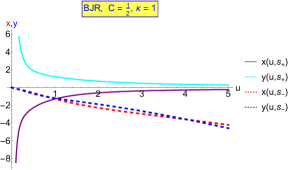
Figure 1: The projections to the transverse plane of the geodesics in BJR coordinates, unfolded to “time” $u$. The trajectories obtained by choosing $s_{+}$ or $s_{-}$ look substantially different.

However they are carried into each other by following the rule (IV.8), see fig.2.

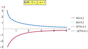
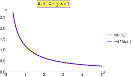
(i)                                                                (ii)

Figure 2: (i) Consistently with (IV.7a) and (IV.7b), changing the parameter $u_{+}\equiv u$ into $u_{-}\equiv u^{-1}$ and multiplying by appropriate $\pm$ signs as in (IV.8) carries the transverse components of a geodesic associated with $s_{+}$ into those associated with $s_{-}$. (ii) For null geodesics the vertical components $v(u_{\pm})$ match also, see (IV.7c) .

Similarly, solving (either numerically or by pulling back from BJR to B coordinates by (II.17)) the transverse equations (III.3) in Brinkmann coordinates yields differently looking geodesics, see fig.3. However combining with the inversion $U\to U^{-1}$ and changing signs appropriately yields identical geodesics, consistently with (IV.11), see fig.4.

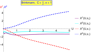
Figure 3: Pulling back to Brinkmann coordinates the transverse components of the BJR geodesics associated with $s_{+}$ or $s_{-}$ [or equivalently, the coefficients $\bm{\beta}$ of the isometries] are different.

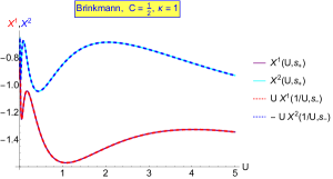
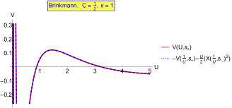
(i)                                                            (ii)

Figure 4: The transverse projections of the geodesics in Brinkmann coordinates are taken into each other under (IV.11).

The Killing vectors are $Y_{V}={\partial}_{V}$ and $Y_{\kappa}$ in (III.11), augmented with those 4 translation-boost type ones in eqns. (III.17) which can be calculated both numerically or analytically using Appendix B.

V.3 A Bianchi VII example: $C=\kappa$

For the value $C=\kappa$ which lies at the edge of the range (I.4), eqn (II.7) yields 4 solutions, $s=\hbox{$\textstyle\frac{1}{2}$}$  (double root) and $s=\hbox{$\textstyle\frac{1}{2}$}(1\pm\sqrt{1-4C^{2}}\big{)}\,.$ Although the latter two are real when $C=\kappa\leq 1/2$ they should nevertheless be discarded because of the Bianchi VII requirement $C=\kappa>1/2$ in (I.4) leaving us with just one (double) real solution, $s=\hbox{$\textstyle\frac{1}{2}$}$; (II.8) yields the auxiliary parameters. The Souriau matrix is,

$$\begin{array}[]{cll}S^{11}&=&\,\frac{2|\kappa|}{\sqrt{4\kappa^{2}-1}}\,\ln u+\frac{1}{4\kappa^{2}-1}\,\sin(\sqrt{4\kappa^{2}-1}\,\ln u)\,,\\[6.0pt] S^{12}=S^{21}&=&\frac{1}{4\kappa^{2}-1}\,\cos(\sqrt{4\kappa^{2}-1}\,\ln u)\,,\\[6.0pt] S^{22}&=&\frac{2|\kappa|}{\sqrt{4\kappa^{2}-1}}\,\ln u-\frac{1}{4\kappa^{2}-1}\,\sin(\sqrt{4\kappa^{2}-1}\,\ln u)\,.\end{array}$$ (V.10)

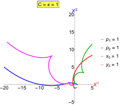
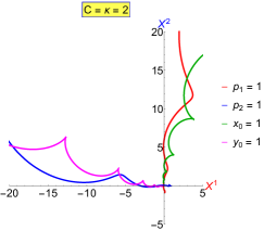
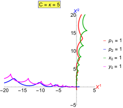
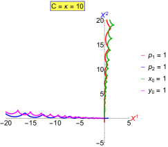
Figure 5: Transverse components of 4-parameter families of “translation-boost type” isometries/geodesics for Bianchi-VII-type Lukash waves. When $C=\kappa\to\infty$ they manifestly “flatten out.

Then (III.17) (resp. (III.3) - (III.4)) yield, for each fixed value of $C=\kappa~{}>~{}{\hbox{$\textstyle\frac{1}{2}$}}$, a 4-parameter family of Killing vectors (resp. geodesics), whose transverse components are plotted in fig.5. Unfolding them to “time” $U$ would indicate that starting from a small initial value $U_{0}>0$, they extend to $U\to\infty$.

To explain the curious “flattening”, we could argue intuitively that for increasingly high frequency $\kappa$ the wave has no “time” to push out the geodesic before pulling it back again. This can also be confirmed analytically. Letting $\kappa\to\infty$ the P matrix (II.19) resp. the Souriau matrix (V.10) become asymptotically linearly polarized (off-diagonal) and resp. diagonal. Inserting their asymptotic values into eqn (B.1) (B.3) (B.5) (B.8) of Appendix B yields the asymptotic behavior

$$Y_{1}\approx\sqrt{U}\,{\partial}_{2},\quad Y_{2}\approx-\sqrt{U}\,{\partial}_{1},\quad Y_{3}\approx(\sqrt{U}\,\ln u)\,{\partial}_{2},\quad Y_{4}\approx(-\sqrt{U}\,\ln u)\,{\partial}_{1}\,.$$ (V.11)

Equivalently, the transverse components of the geodesics are asymptotically

$$X^{1}\approx-\sqrt{U}(p_{y}\,\ln U+y_{0}),\qquad X^{2}\approx\sqrt{U}(p_{x}\,\ln U+x_{0})$$ (V.12)

consistently with fig.5.

VI Global Considerations

The Milne Region. In order to get an insight into the global structure, it may be helpful to consider first the flat limit when no wave is present, i.e., when $C=0$ in Brinkmann coordinates which is Minkowski spacetime, with $-\infty<U<\infty$, $-\infty<V<\infty$. If $U=0$ we have a null-hyperplane separating Minkowski spacetime in two halves, one half to its future, $U>0$, and one to its past $U<0$. If $C\neq 0$ $U=0$ then is singular and we can with no loss of generality restrict $U$ to positive values. Setting $U=u,\,{\bf X}=u{\bf x},\,V=v-\hbox{$\textstyle\frac{1}{2}$}{u}\,{\bf x}^{2}$ allows us to the metric in the form,

$$ds^{2}=2dUdV+d{\bf X}^{2}=2dudv+u^{2}d{\bf x}^{2},$$ (VI.1)

cf. (V.5c). The coordinate transformation is valid only if $U=u>0$ or $U=u<0$ and is singular on the null hyperplane $u=U=0$. The further coordinate change (valid only if $u>0,\,v<0$)

$$u=t\exp(-z)\,,\qquad v=-\hbox{$\textstyle\frac{1}{2}$}t\exp(z)$$ (VI.2)

transforms the metric to

$$ds^{2}=-dt^{2}+t^{2}\Bigl{\{}dz^{2}+e^{-2z}(dx^{2}+dy^{2})\Bigr{\}}\,.$$ (VI.3)

which is the Milne form of the flat Minkowski metric. Let us call this region II, since it is to the future of the region I which is defined as $u>0,\,v>0$.

Since the 3-metric in the braces is of constant negative curvature the spacetime metric is of Friedmann-Lemaître form with $t$ playing the role of cosmic time and $x,y,z$ being comoving coordinates. The 3-metric in braces in (VI.3) is that of the upper-half space model of three-dimensional hyperbolic space $H^{3}$, but as such is not global.

The isometry group of hyperbolic space is $\mathrm{SO}(3,1)$ and (VI.3) makes manifest the Bianchi VII subgroup, together with an additional $\mathrm{SO}(2)$, the so-called LRS action.

The Rindler Region. Having dealt with region II we now return to consideration of region I, that is $v>0$ . We replace (VI.2) by reversing the roles played by of $z$ and $t$,

$$u=\tilde{z}\,\exp({\tilde{t}})\,,\qquad v=\hbox{$\textstyle\frac{1}{2}$}\tilde{z}\,\exp(-\tilde{t})$$ (VI.4)

and find the Rindler form,

$$ds^{2}=d\tilde{z}^{2}+\tilde{z}^{2}\Bigl{\{}-d\tilde{t}^{2}+e^{2\tilde{t}}(dx^{2}+dy^{2})\Bigr{\}}\,.$$ (VI.5)

The metric in braces is Lorentzian and is that of one half of three-dimensional de Sitter spacetime $dS_{3}$. It has constant curvature. In terms of the Carter-Penrose diagram the metric is

$$2dudv=-(dx^{0})^{2}+(dx^{3})^{2}=-\tilde{z}^{2}d\tilde{t}^{2}+d\tilde{z}^{2}$$ (VI.6)

and is valid inside the so called right hand Rindler Wedge $x^{3}>|x^{0}|$. Since

$$x^{0}=\tilde{z}\sinh\tilde{t}\,,\qquad x^{3}=\tilde{z}\cosh\tilde{t}$$ (VI.7)

the timelike curves $\tilde{z}={\rm constant}>0$ are hyperbolae and the orbits of Lorentz boosts about the origin. As a consequence they may consider the world lines of Rindler observers having constant acceleration. The null line $\tilde{t}=\tilde{z}$ is their future horizon and the null line $\tilde{t}=-\tilde{z}$ their past horizon. This should be contrasted with the Milne region II. In that case

$$ds^{2}=2dudv=(dx^{0})^{2}-(dx^{3})^{2}=-dt^{2}+t^{2}dz^{2}$$ (VI.8)

whence

$$x^{0}=t\sinh z\,,\qquad x^{3}=t\cosh z\,.$$ (VI.9)

The curves $z={\rm constant}$ are timelike straight lines through the origin which may be considered the worldlines of Milne’s cosmological observers.

Now we turn to Lukash plane waves. The discussion closely parallels that for Minkowski spacetime given above but using the material developed earlier. We restrict the Lukash metric to positive $U$. Recall that in section II.2 we introduced the coordinates $t$ and $z$ as in (II.12) and cast the metric in Bianchi $VII_{h}$ form as in equations (II.14). This was valid for $u>0,\,v<0$. The orbits of the Bianchi $VII_{h}$ are spacelike. This is sufficient to cover the Milne type region. In order to cover the Rindler type region $u>0,\,v>0$ we cannot use (II.12) but rather introduce coordinates $\tilde{t},\tilde{z}$ by

$$u=\tilde{t}e^{-\frac{\tilde{z}}{2b}}\,,\quad v=\hbox{$\textstyle\frac{1}{2}$}\tilde{t}e^{\frac{\tilde{z}}{2b}}\qquad\text{\small in terms of which}\qquad 2dudv=d{\tilde{t}}^{2}-{\tilde{t}}^{2}\frac{d\tilde{z}^{2}}{4b^{2}}$$ (VI.10)

and so ${\partial}_{\tilde{t}}$ is spacelike and ${\partial}_{\tilde{z}}$ is timelike. Now (II.1) is replaced by

$$ds^{2}=(d\tilde{t})^{2}+g_{ij}(\tilde{t})\lambda^{i}\lambda^{j}\,,$$ (VI.11)

where the invariant one-forms depend on $\tilde{z},x,y$ and the 3-metric $g_{ij}(\tilde{t})$ now has Lorentzian signature $++-$ .

As remarked previously, the pp-wave metric is singular at $u=0$, and therefore we restrict our exploration to $u>0$. In fact, he singularity is of a type called “non-scalar” because no scalar polynomial formed from the Riemann tensor blows up. In fact for pp-waves all scalar polynomials formed from the Riemann tensor vanish identically.

The situation is illustrated by figure 1, p. 406 of Siklos81 and figure 1 on p. 256 of Siklos3 .

VII Conclusion

In this paper we have examined in detail the Lukash plane gravitational wave. Our aim has been to give a self-contained account of its geometry and global structure and to relate it to spatially homogeneous cosmological models.

pp waves admit a generic five dimensional isometry group which acts within the wave fronts BoPiRo ; exactsol ; LL ; Sou73 ; Carroll4GW ; Carrollvs .

The Lukash wave metric has (as do CPP waves) an additional $6$th isometry exactsol ; Carroll4GW ; CPP ; Conf4GW , given in eqn (III.11) (in Brinkmann) or in (III.19) in (BJR). The extra generator takes one out of the wave fronts and the metric becomes homogeneous.

This additional generator actually belongs to a three dimensional Bianchi $VII_{h}$ type subgroup which acts transitively on three dimensional orbits and leads to an intimate connection between gravitational waves and spatially homogeneous cosmological models and thence to the theory of Killing horizons. In BJR coordinates the Bianchi group ${G}_{3}$ consists of two transverse translations plus the VSR-type triple combination GibbonsVSR , cf. (III.18)- (III.19).

In section VI we provide a global picture of the spacetime. The gravitational wave emanates from a singular wave front and splits into two regions which we have dubbed of Milne type and of Rindler type, divided by a Killing horizon.

In the Milne region the orbits of the Bianchi group are spacelike and the spacetime resembles an anisotropic deformation of Milne’s cosmological model. In the Rindler region the orbits are timelike and the spacetime resembles an anisotropic deformation of the Rindler wedge. The involution (I.6) interchanges the singularity at $u=0$ with the conformal infinity at $u=\infty$ as observed in sects IV and VI and reserved for further investigations.

Appendix A: The Bianchi $VII_{h}$ type Group

Here we collect some relevant facts about the Bianchi group $VII_{h}$ exactsol ; EllisMacCallum ; MacCallum . The latter has a matrix representation

$$g(\lambda,\eta)={\left(\begin{array}[]{ccc}e^{i(1-ic)\lambda}&0&\eta\\ 0&1&\lambda\\ 0&0&1\\ \end{array}\right)}$$ (A.1)

where $\lambda\in\mathbb{R}$ and $\eta\in\mathbb{C}$. To obtain a real representation one sets $i={\left(\begin{array}[]{cr}0&-1\\ 1&0\\ \end{array}\right)}$ in the first column and replaces $\eta$ by ${\left(\begin{array}[]{c}\alpha\\ \beta\\ \end{array}\right)}$ with $\alpha,\beta\in\mathbb{R}$. One may verify that

$$g(\lambda_{1},\eta_{1})g(\lambda_{2},\eta_{2})=g(\lambda_{1}+\lambda_{2},e^{i(1-ic)\lambda_{1}}\eta_{2}+\eta_{1})\,.$$ (A.2)

Infinitesimally

$$g ={\left(\begin{array}[]{ccc}1&0&0\\ 0&1&0\\ 0&0&1\\ \end{array}\right)+\lambda\left(\begin{array}[]{ccc}i(1-ic)&0&0\\ 0&0&0\\ 0&0&0\\ \end{array}\right)+\eta\left(\begin{array}[]{ccc}0&0&1\\ 0&0&0\\ 0&0&0\\ \end{array}\right)+\dots}=1+\alpha{\bf e}_{1}+\beta{\bf e}_{2}+\lambda{\bf e}_{3}+\dots$$ (A.3j)

where

$${\bf e}_{1}={\left(\begin{array}[]{cccc}0&0&0&1\\ 0&0&0&0\\ 0&0&0&0\\ 0&0&0&0\end{array}\right)\,,\qquad{\bf e}_{2}=\left(\begin{array}[]{cccc}0&0&0&0\\ 0&0&0&1\\ 0&0&0&0\\ 0&0&0&0\end{array}\right)\,,\qquad{\bf e}_{3}=\left(\begin{array}[]{cccc}c&-1&0&0\\ 1&c&0&0\\ 0&0&0&1\\ 0&0&0&0\end{array}\right)\,.}$$ (A.4)

The ${\bf e}_{1},{\bf e}_{2},{\bf e}_{3}$ form a basis of the Lie algebra $\mathfrak{vii}_{h}$ with commutation relations

$$[{\bf e}_{3},{\bf e}_{1}]=c\,{\bf e}_{1}+{\bf e}_{2}\,,\qquad[{\bf e}_{3},{\bf e}_{2}]=c\,{\bf e}_{2}-{\bf e}_{1}\,.$$ (A.5)

Thus we get

$$g^{-1}dg={\bf e}_{1}\lambda^{1}+{\bf e}_{2}\lambda^{2}+e_{3}\lambda^{3}\,.$$ (A.6)

$\lambda^{i}$ is a basis of left-invariant one-forms given by

$$\lambda^{1} = e^{-c\gamma}(\cos\gamma d\alpha+\sin\gamma d\beta)$$

$$\lambda^{2} = e^{-c\gamma}(\cos\gamma d\beta-\sin\gamma d\alpha)$$ (A.7)

$$\lambda^{3} = d\gamma$$

and the non-trivial Maurer-Cartan relations are

$$d\lambda^{1}=-c\lambda^{3}\wedge\lambda^{1}+\lambda^{3}\wedge\lambda^{2}\,,\qquad d\lambda^{2}=-c\lambda^{3}\wedge\lambda^{2}-\lambda^{3}\wedge\lambda^{1}\,.$$ (A.8)

In terms of structure constants: if

$$[{\bf e}_{i},{\bf e}_{j}]=C_{i}\,^{k}\,{}_{j}{\bf e}_{k}$$ (A.9)

then $d\lambda^{k}=-\hbox{$\textstyle\frac{1}{2}$}C_{i}\,^{k}\,{}_{j}\lambda^{i}\wedge\lambda^{j}\,,$ where

$$C_{3}\,^{1}\,{}_{1}=-C_{1}\,^{1}\,{}_{3}=c\,, C_{3}\,^{2}\,{}_{1}=-C_{1}\,^{2}\,{}_{3}=1$$

$$C_{3}\,^{2}\,{}_{2}=-C_{2}\,^{2}\,{}_{3}=c\,, C_{3}\,^{1}\,{}_{2}=-C_{2}\,^{1}\,{}_{3}=-1\,.$$ (A.10)

The vector fields generating left actions on $VII_{h}$ are obtained by taking $\lambda_{1}$ and $\eta_{1}$ infinitesimal. From (A.2) we find $\delta\eta_{2}=\eta_{1}\,,\,\delta\lambda=\lambda_{1}+i(1-ic)\eta_{i}$ which correspond to:

$$R_{1}={\partial}_{\alpha}\,,\qquad R_{2}={\partial}_{\beta}\,,\qquad R_{3}={\partial}_{\lambda}+\alpha{\partial}_{\beta}-\beta{\partial}_{\alpha}+c(\alpha{\partial}_{\alpha}+\beta{\partial}_{\beta})\,,$$ (A.11)

whence

$$[R_{3},R_{1}]=-cR_{1}-R_{2}\,,\qquad[R_{3},R_{2}]=-cR_{2}+R_{1}\,.$$ (A.12)

In other words,

$$[R_{i},R_{j}]=-C_{i}\,^{k}\,{}_{j}R_{k}\,.$$ (A.13)

Cartan’s formula ${\mathcal{L}}_{V}\omega=d(i_{X}\omega)+i_{X}d\omega$ with $V=R_{i}$ and $\omega=\lambda^{j}$ shows that the one-forms $\lambda^{j}$ are left-invariant, ${\mathcal{L}}_{R_{i}}\lambda^{j}=0\,.$ From (A.10) we deduce that

$$C_{i}\,^{k}\,{}_{k}=(0,0,2c)$$ (A.14)

which confirms that the Bianchi $VII_{h}$ is not non-unimodular, that is, the adjoint representation is not volume-preserving, known in the cosmology literature as class B.

To make contact with (I.5) it is helpful to note that

$$\bigl{(}\lambda^{1}\bigr{)}^{2}+\bigl{(}\lambda^{2}\bigr{)}^{2} =e^{-2c\lambda}(d\alpha^{2}+d\beta^{2})$$ (A.15a)

$$\bigl{(}\lambda^{1}\bigr{)}^{2}-\bigl{(}\lambda^{2}\bigr{)}^{2} =e^{-2c\lambda}(\cos(2\lambda)(d\alpha^{2}-d\beta^{2})+2\sin(2\lambda)d\alpha d\beta)$$ (A.15b)

$$2\lambda^{1}\lambda^{2} =e^{-2c\lambda}(\cos(2\lambda)2d\beta d\alpha-\sin(2\lambda)(d\alpha^{2}-d\beta^{2}))\,$$ (A.15c)

so that

$$k(\lambda^{1})^{2}+k(\lambda^{2})^{2}+(\lambda^{1})^{2}-(\lambda^{2})^{2}=$$

$$\quad e^{-2c\lambda}\Bigr{\{}(k+\cos 2\lambda)d\alpha^{2}+2\sin 2\lambda d\alpha d\beta+(k-\cos 2\lambda)d\beta^{2}\Bigr{\}}\,.$$ (A.16)

Appendix B: “Translation-boost-type” isometries

In the Lukash case the $P$-matrix is known in terms of the Siklos’ parameters (II.7)-(II.8) and spelling out eqn (III.17) yields those 4 “translation-boost-type” isometries in Brinkmann coordinates,

• 2 “translations”

  $$Y_{1}=P_{11}\partial_{1}+P_{21}\partial_{2}-(P_{11}^{\prime}X^{1}+P_{21}^{\prime}X^{2})\partial_{V}\,,$$ (B.1)

  where

  $$P_{11} =\frac{U^{s}}{2}\left[e^{i\alpha}\Big{(}\cosh(\mu/2)U^{-i(\kappa-b)}-\sinh(\mu/2)U^{-i(\kappa+b)}\Big{)}+c.c.\right]\,$$ (B.2a)

  $$P_{21} =\frac{U^{s}}{2}\left[-ie^{i\alpha}\Big{(}\cosh(\mu/2)U^{-i(\kappa-b)}-\sinh(\mu/2)U^{-i(\kappa+b)}\Big{)}+c.c.\right]\,$$ (B.2b)

  and

  $$Y_{2}=P_{12}\partial_{1}+P_{22}\partial_{2}-(P_{12}^{\prime}X^{1}+P_{22}^{\prime}X^{2})\partial_{V}\,,$$ (B.3)

  where

  $$P_{12} =\frac{U^{s}}{2}\left[ie^{i\alpha}\Big{(}\cosh(\mu/2)U^{-i(\kappa-b)}+\sinh(\mu/2)U^{-i(\kappa+b)}\Big{)}+c.c.\right]\,$$ (B.4a)

  $$P_{22} =\frac{U^{s}}{2}\left[e^{i\alpha}\Big{(}\cosh(\mu/2)U^{-i(\kappa-b)}+\sinh(\mu/2)U^{-i(\kappa+b)}\Big{)}+c.c.\right]\,$$ (B.4b)

• These are completed with 2 “boosts”

  $$Y_{3}=(S^{11}P_{11}+S^{12}P_{12})\partial_{1}+(S^{11}P_{21}+S^{12}P_{22})\partial_{2}-(S^{1k}P_{jk})^{\prime}X^{j}\partial_{V}\,,$$ (B.5)

  whose $\partial_{1}$ resp. $\partial_{2}$ components are

  $$S^{11}P_{11}+S^{12}P_{12} = \frac{U^{1-s}}{2}\left[e^{i\alpha}U^{-i(\kappa-b)}\frac{\cosh(\mu/2)(1-2s+2i\kappa)}{(1-2s)(1-2s+2ib)}+c.c\right]\,,\qquad\qquad$$ (B.6)

  $$+ \frac{U^{1-s}}{2}\left[e^{i\alpha}U^{-i(\kappa+b)}\frac{\sinh(\mu/2)(1-2s+2i\kappa)}{(1-2s)(1-2s-2ib)}+c.c\right]\,,$$

  $$S^{11}P_{21}+S^{12}P_{22} = \frac{U^{1-s}}{2}\left[-ie^{i\alpha}U^{-i(\kappa-b)}\frac{\cosh(\mu/2)(1-2s+2i\kappa)}{(1-2s)(1-2s+2ib)}+c.c\right]\,,\qquad\qquad$$ (B.7)

  $$+ \frac{U^{1-s}}{2}\left[-ie^{i\alpha}U^{-i(\kappa+b)}\frac{\sinh(\mu/2)(1-2s+2i\kappa)}{(1-2s)(1-2s-2ib)}+c.c\right]\,.$$

  and by

  $$Y_{4}=(S^{21}P_{11}+S^{22}P_{12})\partial_{1}+(S^{21}P_{21}+S^{22}P_{22})\partial_{2}-(S^{2k}P_{jk})^{\prime}X^{j}\partial_{V}\,,$$ (B.8)

  whose $\partial_{1}$ resp. $\partial_{2}$ components are

  $$S^{21}P_{11}+S^{22}P_{12} = \frac{U^{1-s}}{2}\left[ie^{i\alpha}U^{-i(\kappa-b)}\frac{\cosh(\mu/2)(1-2s+2i\kappa)}{(1-2s)(1-2s+2ib)}+c.c\right]\,\qquad\qquad$$ (B.9)

  $$+ \frac{U^{1-s}}{2}\left[-ie^{i\alpha}U^{-i(\kappa+b)}\frac{\sinh(\mu/2)(1-2s+2i\kappa)}{(1-2s)(1-2s-2ib)}+c.c\right]\,,$$

  $$S^{21}P_{21}+S^{22}P_{22} = \frac{U^{1-s}}{2}\left[e^{i\alpha}U^{-i(\kappa-b)}\frac{\cosh(\mu/2)(1-2s+2i\kappa)}{(1-2s)(1-2s+2ib)}+c.c\right]\,\qquad\qquad$$ (B.10)

  $$+ \frac{U^{1-s}}{2}\left[-e^{i\alpha}U^{-i(\kappa+b)}\frac{\sinh(\mu/2)(1-2s+2i\kappa)}{(1-2s)(1-2s-2ib)}+c.c\right]\,.$$