SF-GRASS: Solver-Free Graph Spectral Sparsification

Abstract.

Recent spectral graph sparsification techniques have shown promising performance in accelerating many numerical and graph algorithms, such as iterative methods for solving large sparse matrices, spectral partitioning of undirected graphs, vectorless verification of power/thermal grids, representation learning of large graphs, etc. However, prior spectral graph sparsification methods rely on fast Laplacian matrix solvers that are usually challenging to implement in practice. This work, for the first time, introduces a solver-free approach (SF-GRASS) for spectral graph sparsification by leveraging emerging spectral graph coarsening and graph signal processing (GSP) techniques. We introduce a local spectral embedding scheme for efficiently identifying spectrally-critical edges that are key to preserving graph spectral properties, such as the first few Laplacian eigenvalues and eigenvectors. Since the key kernel functions in SF-GRASS can be efficiently implemented using sparse-matrix-vector-multiplications (SpMVs), the proposed spectral approach is simple to implement and inherently parallel friendly. Our extensive experimental results show that the proposed method can produce a hierarchy of high-quality spectral sparsifiers in nearly-linear time for a variety of real-world, large-scale graphs and circuit networks when compared with prior state-of-the-art spectral methods.

1. Introduction

Spectral methods are playing increasingly important roles in a wide variety of graph and numerical applications (teng2016scalable, ). Examples include scientific computing and numerical optimization (spielman2014sdd, ; kelner2014almost, ; feng2016spectral, ), graph partitioning and data clustering (lee2014multiway, ; peng2015partitioning, ), machine learning and data mining (kipf2016semi, ; deng2019graphzoom, ), as well as integrated circuit modeling, simulation and verifications (xueqian:tcad15, ; lengfei:tcad15, ; zhiqiang:dac17, ). In particular, latest theoretical breakthroughs in spectral graph theory have led to the development of nearly-linear time spectral graph sparsification (spielman2011spectral, ; feng2016spectral, ; Lee:2017, ; zhuo:dac18, ) and coarsening algorithms (loukas2018spectrally, ; loukas2019graph, ; zhao2018nearly, ; zhao:dac19, ). These techniques can efficiently produce much smaller graphs that well preserve the key spectral properties of the original graph (e.g., the first few eigenvalues and eigenvectors of the graph Laplacian), which in turn has led to much faster algorithms for solving partial differential equations (PDEs) and linear systems of equations (spielman2011spectral, ; peng2013phd, ; zhiqiang:iccad17, ), spectral clustering and graph partitioning (peng2015partitioning, ; lee2014multiway, ; zhuo:dac18, ; zhao:dac19, ), and dimensionality reduction and data visualization (zhao2018nearly, ).

However, prior spectral graph sparsification methods strongly rely on fast Laplacian matrix solvers that are usually challenging to implement in practice and inherently-difficult accelerate on parallel processors. For example, effective-resistance sampling-based spectral sparsification method (spielman2011graph, ) requires multiple Laplacian matrix solutions for computing each edge’s leverage score, while the latest spectral-perturbation based algorithm (feng2020grass, ) leverages a graph-theoretic algebraic multigrid (AMG) solver for computing dominant generalized eigenvectors key to estimating each edge’s spectral importance. As a result, the performance (scalability) of Laplacian matrix solver can become a dominating factor in existing spectral sparsification methods. However, after decades of extensive research studies by theoretical computer scientists, it is still not clear if there exist any practically-efficient (nearly-linear time) and robust Laplacian solvers for general large-scale real-world graphs.

This paper for the first time introduces a solver-free spectral graph sparsification framework (SF-GRASS) by leveraging emerging spectral graph coarsening (zhao:dac19, ) and graph signal processing techniques (shuman2013emerging, ). Our approach first coarsens the original graph into increasingly smaller graphs while preserving the key graph spectral properties. Since spectral graph coarsening (zhao:dac19, ) can be considered as a cascade of low-pass graph filters with decreasing bandwidths, spectrally-critical edges for different ranges of eigenvalues can be effectively identified on coarse-level graphs in a stratified manner. For example, considering a coarsest graph that has only a few (e.g. two) nodes, any graph signals smoothed (low-pass filtered) from random vectors can become good approximations of the Fiedler vector corresponding to the few smallest nontrivial Laplacian eigenvalues; when such vectors are leveraged for recovering spectrally-critical edges using spectral-perturbation based approach similar to the one introduced in (feng2016spectral, ), ultra-sparse spectral graph sparsifiers preserving the smallest few eigenvalues can be efficiently extracted; by iteratively mapping sparsifiers back to each finer level, a hierarchy of spectral sparsifiers with increasing sizes can be incrementally computed for preserving increasing eigenvalues. Our results show SF-GRASS outperforms prior state-of-the-art methods for spectral sparsification considering both efficiency and solution quality. The technical contribution of this work has been summarized as follows:

1. For the first time, we present a solver-free spectral graph sparsification framework (SF-GRASS) by leveraging emerging spectral graph coarsening (zhao:dac19, ) and graph signal processing techniques (shuman2013emerging, ). It can be implemented using simple sparse-matrix-vector multiplications and thus completely addresses the computational challenges in prior methods that strongly reply on efficient graph Laplacian solvers.

2. We introduce a multilevel spectral sparsification framework, which is motivated by the prior graph spectral perturbation analysis approach (feng2016spectral, ). Such a scalable framework allows constructing a hierarchy of spectrally-reduced and sparsified graphs in nearly-linear time, which can become key to accelerating many graph-based numerical computing tasks.

3. By comprehensively comparing with the state-of-the-art method through extensive experiments, we show that in various numerical and graph-related applications, such as solving sparse SDD matrices, and vectorless verification of power grids, SF-GRASS can always obtain high-quality solution while achieving dramatically improved runtime scalability.

The rest of this paper is organized as follows. Section 2 provides a brief introduction to spectral graph sparsification and coarsening problems. In Section 3, a solver-free, multilevel spectral graph sparsification framework is described in detail. Section 4 demonstrates extensive experiment results for a variety of real-world, large-scale matrix and graph problems, which is followed by the conclusion of this work in Section 5.

2. Background

2.1. Graph Laplacians and Quadratic Forms

Consider a weighted, undirected graph $\mathcal{G}=(\mathcal{V},\mathcal{E},\omega)$ with $\mathcal{|V|=N}$ and $\mathcal{|E|=M}$, where $\mathcal{V}$ denotes a set of vertices, $\mathcal{N}$ denotes the number of vertices, $\mathcal{E}$ denotes a set of edges, $\mathcal{M}$ denotes the number of edges, and $\omega$ denotes a weight function that assigns a positive weight to each edge. The adjacency matrix of graph $\mathcal{G}$ can be defined as follows:

(1) $$\mathbf{\mathcal{A}_{\mathcal{G}}}(p,q)=\begin{cases}\omega(p,q)&\text{ if }(p,q)\in\mathcal{E}\\ 0&\text{ if otherwise }.\end{cases}$$

The Laplacian matrix can be computed by $\mathcal{L_{G}}=\mathcal{D_{G}}-\mathcal{A_{G}}$, where $\mathcal{D_{G}}$ is an diagonal matrix with elements $\mathcal{D}_{\mathcal{G}}(p,p)=\sum\limits_{t\neq p}\omega(p,t)$. For any real vector $x\in{\mathbb{R}^{\mathcal{N}}}$, the Laplacian quadratic form of graph $\mathcal{G}$ is defined as: $\mathbf{{x^{\top}}\mathcal{L}_{\mathcal{G}}x}=\sum\limits_{\left({p,q}\right)\in E}{{\omega({p,q})}{{\left({x\left(p\right)-x\left(q\right)}\right)}^{2}}}$.

2.2. Spectral Graph Sparsification

Spectral sparsifier was first introduced by Spielman and Teng (spielman2011spectral, ), which is a strictly stronger notation than the cut sparsifier (benczur1996approximating, ; benczur2015randomized, ). The spectral sparsifier is a weighted subgraph such that the difference of quadratic forms calculated by original graph and the sparsifier is bounded by $(1\pm\epsilon)$, where $\epsilon$ is a constant factor. Given an undirected graph with $\mathcal{N}$ vertices and $\mathcal{M}$ edges, a nearly-linear time algorithm was introduced for building $(1\pm\epsilon)$ spectral sparsifiers with $O(\mathcal{N}\log\mathcal{N}/\epsilon^{2})$ edges in (spielman2011graph, ). Later, Batson, Spielman, and Srivastava (batson2012twice, ) proposed the algorithm for constructing the sparsifier within $O(\mathcal{N}/\epsilon^{2})$ edges. Recently, the state-of-the-art work is given by Lee and Sun (Lee:2017, ) that computes a $(1\pm\epsilon)$ sparsifier with $O(q\mathcal{N}/\epsilon)$ edges in nearly linear time $O\left(\frac{q\mathcal{M}\mathcal{N}^{5/q}}{\epsilon^{4+4/q}}\right)$, where $q$ is an integer greater than $10$.

Another metric for quantifying spectral similarity of two graphs has been proposed by Spielman and Teng (spielman2011graph, ): the subgraph $\mathcal{P}=(\mathcal{V},E)$ is a $\sigma-$spectral sparsifier of the original graph $\mathcal{G}$ if the following inequality holds for any $x\in{\mathbb{R}^{\mathcal{N}}}$

(2) $$\frac{1}{\sigma}{x^{\top}}\mathcal{L}_{\mathcal{G}}x\leq{x^{\top}}\mathcal{L}_{\mathcal{P}}x\leq\sigma{x^{\top}}\mathcal{L}_{\mathcal{G}}x,$$

where the relative condition number is defined as $\kappa(\mathcal{L}_{\mathcal{G}},\mathcal{L}_{\mathcal{P}})\leq\sigma^{2}$. It indicates that a smaller relative condition number corresponds to a higher spectral similarity.

2.3. Spectral Graph Coarsening

Graph coarsening (reduction) not only reduces the number of edges but also aggregates nodes to form smaller number of nodes for graph approximation. It was at heuristics level until Loukas, and Vandergheynst (loukas2018spectrally, ; loukas2019graph, ) developed a theoretical framework which guarantees that the spectral properties of coarsened graphs can approximate the original ones under some restricted circumstances.

3. SF-GRASS: Solver-Free Graph Spectral Sparsification

The proposed Solver-Free Graph Spectral Sparsification (SF-GRASS) framework is built upon a multilevel spectral graph coarsening scheme, which allows constructing multilevel spectral sparsifiers in nearly-linear time. Given an undirected graph $\mathcal{G}=\mathcal{G}_{0}$, a series of reduced graphs $\mathcal{G}_{1},\mathcal{G}_{2},...,\mathcal{G}_{l_{f}}$ will be generated through a spectral coarsening procedure with the corresponding node sizes denoted by $\mathcal{N}_{0},\mathcal{N}_{1},...,\mathcal{N}_{l_{f}}$, where $\mathcal{N}_{0}>\mathcal{N}_{1}>...>\mathcal{N}_{l_{f}}$. Once the the coarsened graphs are constructed, the spectral sparsifier $\mathcal{P}_{l}$ of the coarsened graph $\mathcal{G}_{l}$ at level $l$ will be extracted by the spectral perturbation approach introduced in (feng2016spectral, ), where $l=l_{f},l_{f-1},...,0$, and $\mathcal{P}_{0}=\mathcal{P}$ is defined as the spectral sparsifier for the original graph $\mathcal{G}$. For the sake of simplicity, all the symbols used in this paper are summarized in Table 1.

Table 1. Summary of symbols used in the paper ($l=0,1,...,{l_{f}},i=1,...,\mathcal{N}_{l}$).

symbols	description	symbols	description
$\mathcal{G}_{l}=(\mathcal{V}_{l},\mathcal{E}_{l})$	an undirected graph at level $l$	$\mathcal{P}_{l}=(V_{l},E_{l})$	the sparsifier of $\mathcal{G}_{l}$
$\mathcal{V}_{l}$	node set at level $l$	$\mathcal{V}_{l}$	node set at level $l$
$\mathcal{E}_{l}$	edge set of $\mathcal{G}_{l}$	${E}_{l}$	edge set of $\mathcal{P}_{l}$
${\omega_{l}(p,q)}$	edge weight of node $(p,q)$ for $\mathcal{G}_{l}$	$\omega_{l}(p,q)$	edge weight of node $(p,q)$ for $\mathcal{P}_{l}$
$\mathcal{N}_{l}=|\mathcal{V}_{l}|$	number of nodes	$\mathcal{N}_{l}$	number of nodes
$\mathcal{M}_{l}=|\mathcal{E}_{l}|$	number of edges in $\mathcal{G}_{l}$	${M}_{l}=|E_{l}|$	number of edges in $\mathcal{P}_{l}$
$\mathcal{L}_{\mathcal{G}_{l}}$	Laplacian of graph $\mathcal{G}_{l}$	$\mathcal{L}_{\mathcal{P}_{l}}$	Laplacian of graph $\mathcal{P}_{l}$
$\mathcal{A}_{\mathcal{G}_{l}}$	adjacency matrix of graph $\mathcal{G}_{l}$	$\mathcal{A}_{\mathcal{P}_{l}}$	adjacency matrix of graph $\mathcal{P}_{l}$
$\lambda_{l}^{(i)}$	eigenvalues of $\mathcal{L}_{\mathcal{G}_{l}}$	$\tilde{\lambda}_{l}^{(i)}$	eigenvalues of $\mathcal{L}_{\mathcal{P}_{l}}$
$u_{l}^{(i)}$	eigenvectors of $\mathcal{L}_{\mathcal{G}_{l}}$	$\tilde{u}_{l}^{(i)}$	eigenvectors of $\mathcal{L}_{\mathcal{P}_{l}}$
$S^{(i)}_{l-1}$	node aggregation set at level $l-1$ with respect to the single node $i$ at level $l$

3.1. Overview of Our Approach

Recent research in graph signal processing (GSP) (shuman2013emerging, ) shows that for undirected graphs the smaller eigenvalues and corresponding eigenvectors of its Laplacian are associated to the global structure (long-range distances) of the underlying graph, while the higher eigenvalues and corresponding eigenvectors encode the local structure of the graph. Since spectral sparsification aims to approximate the first few eigenvalues and eigenvectors of the original Laplacian with the minimum number of edges, it can be regarded as a low-pass filter on graphs for removing redundant edges. Spectral sparsification usually involves two steps: the first step is to generate a low-stretch spanning tree (LSST) from the original graph using star or petal decompositions (elkin2008lower, ; abraham2012, ); the next step is to identify and recover spectrally-critical off-tree edges into the LSST to drastically reduce the condition number, and thereby minimizing the spectral mismatch (feng2020grass, ). However, prior spectral sparsification methods (spielman2011graph, ; feng2016spectral, ) usually require solving linear systems of equations with Laplacian solvers, which can still be computationally challenging for large problems.

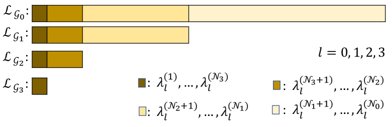
Figure 1. Eigenvalue distributions of $\mathcal{L}_{\mathcal{G}_{l}}$

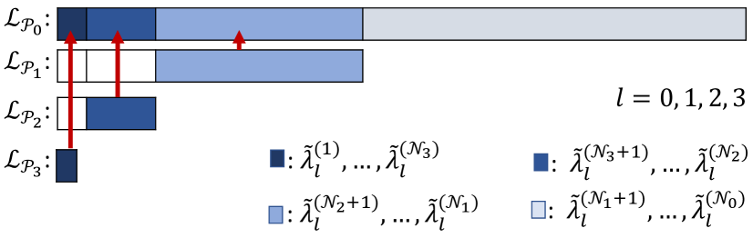
Figure 2. Eigenvalue distributions of $\mathcal{L}_{\mathcal{P}_{l}}$

In this work, we propose a solver-free, multilevel spectral sparsification scheme to generate a hierarchy of increasingly smaller spectral sparsifiers. As aforementioned, given an undirected graph $\mathcal{G}_{0}=\mathcal{G}$, a series of coarsened graphs $\mathcal{G}_{1},\mathcal{G}_{2},...,\mathcal{G}_{l_{f}}$ will be generated via the multilevel spectral graph coarsening scheme introduced in (zhao:dac19, ), where $\mathcal{G}_{l_{f}}$ denotes the coarsest graph. It can be shown that the Laplacian of $\mathcal{G}_{l}$ can well preserve the low eigenvalues and eigenvectors of the finer graphs $\mathcal{G}_{l-1}$, … , $\mathcal{G}_{1}$, $\mathcal{G}_{0}$ (loukas2018spectrally, ; loukas2019graph, ). For example, Figure 2 shows the eigenvalue distributions of the Laplacian matrices corresponding to four consecutive coarse-level graphs, implying that the eigenvalues $\left(\lambda_{l}^{1},...,\lambda_{l}^{\mathcal{N}_{3}}\right)$ of $\mathcal{L}_{\mathcal{G}_{3}}$ will approximately match the smallest eigenvalues of $\mathcal{L}_{\mathcal{G}_{2}}$, $\mathcal{L}_{\mathcal{G}_{1}}$ and $\mathcal{L}_{\mathcal{G}_{0}}$. In other words, $\mathcal{L}_{\mathcal{G}_{3}}$ will always approximately preserve the key spectral (structural) properties of $\mathcal{L}_{\mathcal{G}_{0}}$ after coarsening. Similarly, eigenvalues $\left(\lambda_{l}^{\mathcal{N}_{3}+1},...,\lambda_{l}^{\mathcal{N}_{2}}\right)$ of $\mathcal{L}_{\mathcal{G}_{2}}$ will approximately match the first few eigenvalues of $\mathcal{L}_{\mathcal{G}_{1}}$ and $\mathcal{L}_{\mathcal{G}_{0}}$. Compared to $\mathcal{G}_{3}$ and $\mathcal{G}_{2}$, $\mathcal{G}_{1}$ will retain more local information of $\mathcal{G}_{0}$ by approximately preserving the moderate to large eigenvalues of $\mathcal{L}_{\mathcal{G}_{0}}$. Consequently, spectral coarsening is creating a hierarchy of smaller graphs that can be considered as a cascade of low-pass graph filters with gradually decreasing bandwidths: the finest graph always retains the highest bandwidth, whereas the coarsest graph only retains the lowest bandwidth. The theoretical proofs for the multilevel spectral preservation via graph coarsening are provided in Section 3.3.

Once the series of reduced graphs have been obtained via spectral coarsening, we will be able to effectively exploit them for extracting a hierarchy of ultra-sparse spectral sparsifiers. In the following, we show detailed steps for constructing spectral sparsifiers $\mathcal{P}_{l}$ at each level $l=l_{f},...,1,0$, such that each $\mathcal{P}_{l}$ will be spectrally-similar to $\mathcal{G}_{l}$. Unlike the spectral coarsening step that starts at the finest-level (original) graph, SF-GRASS will start from the coarsest-level graph $\mathcal{G}_{l_{f}}$ and aims to approximate eigenvalues and eigenvectors (in an ascending order) through a stratified scheme: when $\mathcal{G}_{l_{f}}$ is sufficiently small, we can always efficiently extract the spectral sparsifier $\mathcal{P}_{l_{f}}$ for level ${l_{f}}$, leading to good approximation of the first few eigenvalues (eigenvectors); then we will map $\mathcal{P}_{l_{f}}$ to the finer level to facilitate the construction of the next-level sparsifier $\mathcal{P}_{l_{f}-1}$ so that higher eigenvalues (eigenvectors) can be approximated. The proposed approach SF-GRASS strives to incrementally construct a series of increasingly finer spectral sparsifiers, as shown in Figure 2. After iteratively applying the above procedure for all levels, the spectral sparsifier $\mathcal{P}_{0}$ for the original graph can be efficiently constructed to well preserve the key spectral properties of $\mathcal{G}_{0}$.

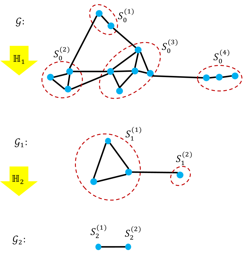
Figure 3. Graph spectral coarsening via local embedding

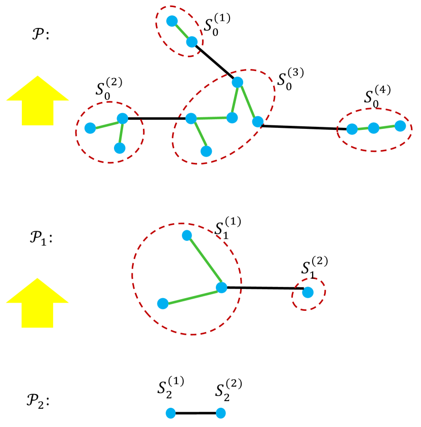
Figure 4. Sparsifier backward mapping

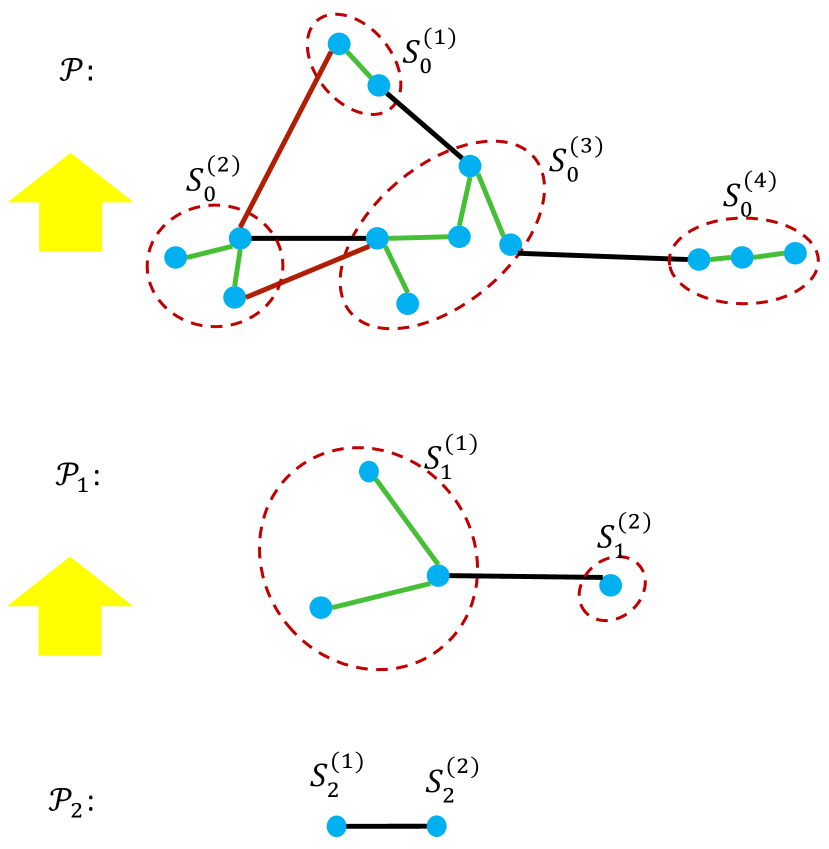
Figure 5. Spectrally-critical edge identification

3.2. Spectral Coarsening via Local Embedding

As shown in Figure 5, an induced subgraph $\mathcal{F}^{(i)}_{l-1}$ can be constructed with the node aggregation set $\mathcal{S}^{(i)}_{l-1}$ and the edge set $\mathcal{E}_{l-1}(\mathcal{S}^{(i)}_{l-1})$ that includes edges $(p,q)$ in $\mathcal{E}_{l-1}$ with both of the nodes p and q included in the set $\mathcal{S}^{(i)}_{l-1}$. The induced subgraphs are strongly-connected components in $\mathcal{G}_{l-1}$, which will be aggregated into a single node of the coarser graph. Next, we create a node-mapping matrix $\mathbb{H}_{l}$ that allows constructing $\mathcal{G}_{l}$ given the finer graph $\mathcal{G}_{l-1}$ with the following equation:

(3) $$\mathcal{L}_{\mathcal{G}_{l}}:=\mathbb{H}_{l}^{\mp}\mathcal{L}_{\mathcal{G}_{l-1}}\mathbb{H}_{l}^{+},\textbf{ and }x_{l}:=\mathbb{H}_{l}x_{l-1},~{}~{}\textbf{for}~{}l=1,2,...,l_{f},$$

where $\mathbb{H}_{l}\in\mathbb{R}^{\mathcal{N}_{l}\times\mathcal{N}_{l-1}}$, $x_{l}\in\mathbb{R}^{\mathcal{N}_{l}\times 1}$, and $\mathbb{H}_{l}^{\top},\mathbb{H}_{l}^{+},\mathbb{H}_{l}^{\mp}$ denote the transpose, pseudoinverse, and transposed pseudoinverse of $\mathbb{H}_{l}$, respectively. $\mathbb{H}_{l},\mathbb{H}_{l}^{+}$ can be created as follows (loukas2019graph, ):

(4) $$\mathbb{H}_{l}(i,p)=\begin{cases}\frac{1}{|\mathcal{S}^{(i)}_{l-1}|}&\text{ if node p}\in\mathcal{S}_{l-1}^{(i)}\\ 0&\text{ if otherwise }.\end{cases}$$

(5) $$\mathbb{H}^{+}_{l}(p,i)=\begin{cases}1&\text{ if node p}\in\mathcal{S}_{l-1}^{(i)}\\ 0&\text{ if otherwise. }\end{cases}$$

When creating a coarsening framework, the core task is to cluster the graph into aggregation sets so that we can define matrix $\mathbb{H}_{l}$. To preserve important spectral properties (e.g., the first few eigenvalues and eigenvectors of the graph Laplacian) on the coarsened graphs, one naive approach is to embed the original graph into a $K$-dimensional space using the first $K$ nontrivial Laplacian eigenvectors. Then, the nodes that are close to each other in the embedding space can be aggregated for forming a coarser graph. However, such a scheme requires calculating the Laplacian eigenvectors, which will be extremely expensive for large graphs.

To achieve good efficiency, SF-GRASS leverages a linear-time local spectral embedding scheme based on low-pass filtering of random graph signals (zhao:dac19, ; deng2019graphzoom, ). Let $X_{l}=[x_{l}^{(1)},x_{l}^{(2)},...,x_{l}^{(K)}]$, where $x_{l}^{(i)}\in\mathbb{R}^{\mathcal{N}_{l}\times 1}$ denote the test vectors computed by applying a few steps of Gaussian-Seidel relaxations for solving the linear system of equations $\mathcal{L}_{\mathcal{G}_{l}}x_{l}^{(i)}=0$ for i = 1, …, K with $K$ initial random vectors that are orthogonal to the all-one vector (livne2012lean, ). The above smoothing procedure can be regarded as a low-pass filtering process applied to $K$ random graph signals. The resultant $K$ smoothed test vectors will consist of linear combinations of the first few Laplacian eigenvectors, and thus can be subsequently leveraged for spectral graph embedding.

Since modern graph signal processing (GSP) based filtering functions are dominated by SpMV operations that are massively-parallel-friendly, the local spectral embedding scheme can be effectively accelerated on modern parallel computing platforms, such as CPUs, GPUs, and FPGAs (steinberger2017globally, ; hong2018efficient, ).

3.3. Spectral Similarity Between Coarse Graphs

After finding the $\mathbb{H}_{l}$, will Eq (2) still hold between $\mathcal{G}_{l}$ and $\mathcal{G}_{l-1}$? If yes, how does the smaller graph $\mathcal{G}_{l}$ spectrally preserve the finer graph $\mathcal{G}_{l-1}$? How will $\mathbb{H}_{l}$ affect the spectral properties of $\mathcal{G}_{l}$? For the above questions, we provide detailed explanation through the following comprehensive theoretical analysis. Let $\lambda_{l}^{(1)},\lambda_{l}^{(2)},..,\lambda_{l}^{(\mathcal{N}_{l})}$, and $u_{l}^{(1)},u_{l}^{(2)},...,u_{l}^{(\mathcal{N}_{l})}$ denote the non-decreasing eigenvalues and their corresponding eigenvectors for $\mathcal{L}_{\mathcal{G}_{l}}$. The restricted spectral similarity (loukas2019graph, ) is defined as follows

(6) $$\frac{1}{\sigma_{l-1}}\|x_{l-1}\|_{\mathcal{L}_{\mathcal{G}_{l-1}}}\leq\|x_{l}\|_{\mathcal{L}_{\mathcal{G}_{l}}}\leq\sigma_{l-1}\|x_{l-1}\|_{\mathcal{L}_{\mathcal{G}_{l-1}}},~{}\forall x_{l-1}\in U^{k}_{l-1},$$

where $U^{k}_{l-1}=\left[u_{l-1}^{(1)},u_{l-1}^{(2)},...,u_{l-1}^{(k)}\right]$ includes the first $k$ eigenvectors of $\mathcal{L}_{\mathcal{G}_{l-1}}$. The restricted spectral similarity can also be denoted as the $(U^{k}_{l-1},\sigma_{l-1})$-spectral similarity. If $\mathcal{L}_{\mathcal{G}_{l-1}}$ and $\mathcal{L}_{\mathcal{G}_{l}}$ are $(U^{k}_{l-1},\sigma_{l-1})$-similar, we have

(7) $$\gamma_{1}\lambda_{l-1}^{(i)}\leq\lambda_{l}^{(i)}\leq\gamma_{2}{\small{\frac{(1+\epsilon)^{2}}{1-\tau\epsilon^{2}}}}\lambda_{l-1}^{(i)}\;,\;\;i=1\;,\cdots\;,\;\mathcal{N}_{l}$$

where $\tau=\lambda^{(k)}_{l-1}/\lambda^{(2)}_{l-1},\epsilon=(\sigma_{l-1}^{2}-1)/(\sigma_{l-1}^{2}+1)$ and $\sigma_{l-1}\leq(\frac{1+\sqrt{\tau}}{1-\sqrt{\tau}})^{\frac{1}{2}}$. $\gamma_{1},\gamma_{2}$ will be the smallest and largest eigenvalues of $(\mathbb{H}_{l}\mathbb{H}_{l}^{\top})^{-1}$. Therefore, the spectral similarity between $\lambda_{l-1}^{(i)}$ and $\lambda_{l}^{(i)}$ can be controlled by $\sigma_{l-1}$. The canonical angles between the principal eigenspace of $\mathcal{L}_{\mathcal{G}_{l-1}}$ and $\mathcal{L}_{\mathcal{G}_{l}}$ are defined as follows:

(8) $$\Theta(U^{k}_{l-1},\mathbb{H}_{l}^{\top}U^{k}_{l})=\textbf{arccos}(U^{k\top}_{l-1}\mathbb{H}_{l}^{\top}U^{k}_{l}U^{k\top}_{l}\mathbb{H}_{l}U^{k}_{l-1})^{-\frac{1}{2}}.$$

Consequently, a smaller canonical angles implies a higher similarity between two eigenspaces.

3.4. Sparsifier Backward Mapping

We aim to iteratively find spectral sparsifiers for achieving desired spectral similarity or relative condition numbers $\kappa(\mathcal{L}_{\mathcal{G}},\mathcal{L}_{\mathcal{P}})=\sigma_{l}^{2}$, $l=l_{f}$,…,0. To this end, we will first extract an LSST, and subsequently, add extra off-tree edges to form the sparsifier at the coarsest level. Next, sparsifiers at finer levels can be obtained by iteratively mapping the coarser sparsifiers via the procedures illustrated in Figures 5 and 5, where $\mathcal{P}$, $\mathcal{P}_{1}$, $\mathcal{P}_{2}$ denote the sparsifiers of $\mathcal{G}$, $\mathcal{G}_{1}$, $\mathcal{G}_{2}$, respectively. $\mathcal{P}_{l}$ and $\mathcal{G}_{l}$ share the same aggregation sets $S_{l-1}^{(i)}$. $\mathcal{P}_{l}$ is the series of coarsened graphs for $\mathcal{P}$ where $l=1,2$. In the following, we describe how to map two types of edges in the proposed sparsifier backward mapping procedure:

• Inner-cluster Edges. We can conveniently locate all the inner-cluster nodes and edges within each aggregation set according to $\mathbb{H}_{l}$ and $\mathcal{G}_{l-1}$. Since each of the aggregation sets is a strongly-connected component, we can extract an LSST for each aggregation set (highlighted by the red dash line in Figure 5). Since each aggregation set size is pretty small, LSSTs can be well approximated using all-pairs shortest-path trees or maximum spanning trees (MSTs).

• Inter-cluster Edges. We could get all the inter-cluster edges between these aggregation sets in the graph $\mathcal{G}_{l-1}$ and only keep the edges with the largest weights in $\mathcal{P}_{l-1}$. As a result, all the aggregation sets will be connected through inter-cluster edges in $\mathcal{P}_{l-1}$, forming a good spectral sparsifier for $\mathcal{G}_{l-1}$ (as shown in Figure 5).

3.5. Spectrally-Critical Edges Identification

To further improve the spectral approximation in sparsifiers, additional spectrally-critical off-tree edges need to be identified and added into the latest sparsifiers. Specifically, $O(\frac{\mathcal{M}_{l}\log\log\mathcal{N}_{l}}{\sigma^{2}})$ spectrally-critical off-tree edges need to be added into LSSTs to obtain a $\sigma$-similar spectral sparsifier $\mathcal{P}_{l}$ for $\mathcal{G}_{l}$. Let $\tilde{u}_{l}^{(i)}$ denote the $i$-th eigenvector of $\mathcal{L}_{\mathcal{P}_{l}}$ corresponding to the $i$-th eigenvalue ${\tilde{\lambda}_{l}^{(i)}}$ that satisfies:

(9) $$\mathcal{L}_{\mathcal{P}_{l}}\tilde{u}_{l}^{(i)}=\tilde{\lambda}_{l}^{(i)}\tilde{u}_{l}^{(i)},$$

then we have the following eigenvalue perturbation analysis:

(10) $$\left({\mathcal{L}_{\mathcal{P}_{l}}+\delta\mathcal{L}_{\mathcal{P}_{l}}}\right)\left({{\tilde{u}_{l}^{(i)}}+\delta{\tilde{u}_{l}^{(i)}}}\right)=\left({{\tilde{\lambda}_{l}^{(i)}}+\delta{\tilde{\lambda}_{l}^{(i)}}}\right)\left({{\tilde{u}_{l}^{(i)}}+\delta{\tilde{u}_{l}^{(i)}}}\right),$$

where a perturbation $\delta\mathcal{L}_{\mathcal{P}_{l}}$ that includes a new edge connection is applied to $\mathcal{L}_{\mathcal{P}_{l}}$, resulting in perturbed eigenvalues and eigenvectors ${\tilde{\lambda}_{l}^{(i)}}+\delta{\tilde{\lambda}_{l}^{(i)}}$ and ${\tilde{u}_{l}^{(i)}}+\delta{\tilde{u}_{l}^{(i)}}$ for $i=1,...,\mathcal{N}_{l}$, respectively. Keeping only the first-order terms leads to:

(11) $${\mathcal{L}_{\mathcal{P}_{l}}}\delta{\tilde{u}_{l}^{(i)}}+{\delta\mathcal{L}_{\mathcal{P}_{l}}}{\tilde{u}_{l}^{(i)}}={{\tilde{\lambda}_{l}^{(i)}}{\delta{\tilde{u}_{l}^{(i)}}}+\delta{\tilde{\lambda}_{l}^{(i)}}}{{\tilde{u}_{l}^{(i)}}}.$$

Expressing $\delta\tilde{u}_{l}^{(i)}$ in terms of the original eigenvectors $\tilde{u}_{l}^{(j)}$ for $j=1,...,\mathcal{N}_{l}$ leads to:

(12) $${\delta{\tilde{u}_{l}^{(i)}}}=\sum\limits_{j=1}^{\mathcal{N}_{l}}{{\alpha_{j}}{\tilde{u}_{l}^{(j)}}}.$$

Substituting (12) into (11) leads to:

(13) $${\mathcal{L}_{\mathcal{P}_{l}}}\sum\limits_{j=1}^{\mathcal{N}_{l}}{{\alpha_{j}}{\tilde{u}_{l}^{(j)}}}+{\delta\mathcal{L}_{\mathcal{P}_{l}}}{\tilde{u}_{l}^{(i)}}={{\tilde{\lambda}_{l}^{(i)}}\sum\limits_{j=1}^{\mathcal{N}_{l}}{{\alpha_{j}}{\tilde{u}_{l}^{(j)}}}+\delta{\tilde{\lambda}_{l}^{(i)}}}{{\tilde{u}_{l}^{(i)}}}.$$

Multiplying ${\tilde{u}_{l}^{(i)\top}}$ to both sides of (13) results in:

(14) $$\begin{split}&{{\tilde{u}_{l}^{(i)\top}}}{\mathcal{L}_{\mathcal{P}_{l}}}\sum\limits_{j=1}^{\mathcal{N}_{l}}{\alpha_{j}}{\tilde{u}_{l}^{(j)}}+{\tilde{u}_{l}^{(i)\top}}\delta\mathcal{L}_{\mathcal{P}_{l}}\tilde{u}_{l}^{(i)}\\ &={{\tilde{\lambda}_{l}^{(i)}}{\tilde{u}_{l}^{(i)\top}}\sum\limits_{j=1}^{\mathcal{N}_{l}}{{\alpha_{j}}{\tilde{u}_{l}^{(j)}}}+\delta{\tilde{\lambda}_{l}^{(i)}}}{\tilde{u}_{l}^{(i)\top}}{\tilde{u}_{l}^{(i)}}.\end{split}$$

Since $\tilde{u}_{l}^{(i)}$ for $i=1,...,\mathcal{N}_{l}$ are unit-length, mutually-orthogonal eigenvectors, we have:

(15) $$\begin{split}&{\tilde{u}_{l}^{(i)\top}}{\mathcal{L}_{\mathcal{P}_{l}}}\sum\limits_{j=1}^{\mathcal{N}_{l}}{{\alpha_{j}}{\tilde{u}_{l}^{(j)}}}={\alpha_{i}}{\tilde{u}_{l}^{(i)\top}}{\mathcal{L}_{\mathcal{P}_{l}}}{{\tilde{u}}}_{l}^{(i)},\\ &{\tilde{\lambda}_{l}^{(i)}}{\tilde{u}_{l}^{(i)\top}}\sum\limits_{j=1}^{\mathcal{N}_{l}}{\alpha_{j}}{\tilde{u}_{l}^{(j)}}={\alpha_{i}}{\tilde{u}_{l}^{(i)\top}}{\tilde{\lambda}_{l}^{(i)}}{\tilde{u}_{l}^{(i)}}.\end{split}$$

Then the eigenvalue perturbation due to ${\delta\mathcal{L}_{\mathcal{P}_{l}}}$ is given by:

(16) $$\delta{\tilde{\lambda}_{l}^{(i)}}=\omega({p,q})\left({{{\tilde{u}_{l}^{(i)\top}}e_{p,q}}}\right)^{2}.$$

Therefore, if an edge $(p,q)$ has a large $\omega(p,q)\left({{{{\tilde{u}_{l}^{(i)\top}}}e_{p,q}}}\right)^{2}$ value, it is considered spectrally critical to $\tilde{\lambda}_{l}^{(i)}$. In other words, including this edge into the latest sparsifier will significantly perturb the Laplacian eigenvalue $\tilde{\lambda}_{l}^{(i)}$ and eigenvector $\tilde{u}_{l}^{(i)}$. Construct a subspace matrix for $K$-dimensional spectral graph embedding using the first $K$ Laplacian eigenvectors as follows:

(17) $$U=\left[\tilde{u}_{l}^{(1)},\tilde{u}_{l}^{(2)},...,\tilde{u}_{l}^{(K)}\right],$$

then the overall $K$-eigenvalue perturbation $\Delta_{K}$ becomes

(18) $$\Delta_{K}=\sum\limits_{i=1}^{{K}}\delta{\tilde{\lambda}_{l}^{(i)}}=\omega({p,q})\left(U^{\top}e_{p,q}\right)^{2},$$

which is similar to the effective-resistance edge sampling probability (spielman2011graph, ) computed by $P=\omega({p,q})R^{eff}_{p,q}$ when $K=\mathcal{N}_{l}$, considering the close connection between the spectral embedding distance $\left(U^{\top}e_{p,q}\right)^{2}$ and the effective resistance distance computed by

(19) $$R^{eff}_{p,q}=\left(U_{eff}^{\top}e_{p,q}\right)^{2},~{}~{}~{}\text{where~{}~{}~{}}U_{eff}=\left[\frac{\tilde{u}_{l}^{(1)}}{\sqrt{\tilde{\lambda}_{l}^{(i)}}},...,\frac{\tilde{u}_{l}^{(\mathcal{N}_{l})}}{\sqrt{\tilde{\lambda}_{l}^{(\mathcal{N}_{l})}}}\right].$$

Instead of computing exact Laplacian eigenvectors for identifying spectrally-critical edges, we will adopt the local spectral embedding approach described in Section 3.2 for approximately computing the spectral embedding distance $\left(U^{\top}e_{p,q}\right)^{2}$. Consequently, we can compute spectral criticalities for all candidate edges in linear time using only a few times of sparse-matrix-vector multiplications.

3.6. Algorithm Flow and Complexity

Algorithm 1 ${\mathcal{P}}$ = SF-GRASS(${\mathcal{G}}$, $\sigma$)

1:  $\mathcal{P}_{l}=\emptyset$ for $l=0,...,l_{f}$;

2:  [${\mathcal{G}_{1}},...,{\mathcal{G}_{l_{f}}};\mathbb{H}_{1},...,\mathbb{H}_{l_{f}}$] = Multilevel$\_$spectral$\_$graph$\_$reduction (${\mathcal{G}}$);

3:  ${\mathcal{P}_{l_{f}}}={\mathcal{G}_{l_{f}}}$; $l=l_{f}$

4:  while  $l\geq 1$ do

5:     for each node $i\in\mathcal{V}_{l}$ do

6:        Find the induced subgraph $\mathcal{F}_{l-1}^{(i)}$ formed by the nodes set $\mathcal{S}_{l-1}^{(i)}$ in $\mathcal{G}_{l-1}$ ;

7:        Extract the LSST $\mathcal{T}_{l-1}^{(i)}$ of $\mathcal{F}_{l-1}^{(i)}$ ;

8:        $\mathcal{P}_{l-1}=\mathcal{P}_{l-1}\cup\mathcal{T}_{l-1}^{(i)}$;

9:     end for

10:     for each edge ${(p,q)}\in\mathcal{}{E}_{l}$ do

11:         Node set $s_{p}=S_{l-1}^{(p)}$, node set $s_{q}=S_{l-1}^{(q)}$; Find the edge with maximum weight between $s_{p}$ and $s_{q}$, and add the edge into $\mathcal{P}_{l-1}$ ;

12:     end for

13:     Embed $\mathcal{G}_{l-1}$ to $K$-dimensional space $X_{l-1}=[x_{l-1}^{(1)},x_{l-1}^{(2)},...,x_{l-1}^{(K)}]$;

14:     For each subgraph edge $(p,q)\in(\mathcal{E}_{l-1}-E_{l-1})$, calculate the edge distortion $d(p,q)\propto{\omega_{l-1}(p,q)}\left(X^{\top}_{l-1}e_{p,q}\right)^{2}$;

15:     Include top few edges with large distortion into $\mathcal{P}_{l-1}$;

16:     $l=l-1$

17:  end while

18:  let ${\mathcal{P}}={\mathcal{P}_{0}}$ and return graph ${\mathcal{P}}$;

Algorithm 1 shows the algorithm flow for the proposed SF-GRASS framework. The complexity of spectral graph coarsening is $O(|\mathcal{E}_{l}|)$ for each level, the complexity of backward graph mapping procedure is $O(|\mathcal{E}_{l}|)$ for each level $l$, and the complexity of off-subgraph identification is $O(|\mathcal{E}_{l}|)$ for each level $l$. If the spectral coarsening step will produce $O(\log|\mathcal{V}|)$ graphs with a fixed coarsening ratio for two consecutive levels, the overall runtime complexity of SF-GRASS is nearly linear for an input graph $\mathcal{G}=(\mathcal{V},\mathcal{E},\omega)$.

4. Experimental results

The proposed spectral sparsification algorithm has been implemented in Matlab and $C$++. The test cases used in this paper have been selected from a great variety of matrices that have been used in circuit simulation, finite element analysis, machine learning, and data mining applications. If the original matrix is not a graph Laplacian, it will be converted into a graph Laplacian by setting each edge weight using the absolute value of each nonzero entry in the lower triangular matrix; if edge weights are not available in the original matrix file, a unit edge weight will be assigned to all edges. All of our experiments have been conducted using a single CPU core of a computing platform running 64-bit RHEW 7.2 with a $2.67$GHz 12-core CPU and $50$ GB memory. Several test cases have been tested in the experiments.

4.1. SF-GRASS for Spectral Graph Sparsification

Table 2. Comparison of spectral sparsification results between SF-GRASS and GRASS.

Test cases	$\mathcal{N}$	$\mathcal{M}$	GRASS			SF-GRASS
			$T_{grass}$	$\frac{|\mathcal{E}_{off}|}{\mathcal{N}}$	$\kappa(\mathcal{L}_{\mathcal{G}},\mathcal{L}_{\mathcal{P}})$	$T_{r}$	$T_{spar}$	$\frac{|\mathcal{E}_{off}|}{\mathcal{N}}$	$\kappa(\mathcal{L}_{\mathcal{G}},\mathcal{L}_{\mathcal{P}})$	$\kappa(\mathcal{L}_{\mathcal{G}},\mathcal{L}_{\mathcal{S}})$	$\frac{\kappa(\mathcal{L}_{\mathcal{G}},\mathcal{L}_{\mathcal{S}})}{\kappa(\mathcal{L}_{\mathcal{G}},\mathcal{L}_{\mathcal{P}})}$
fe$\_$4elt	$1.1E4$	$3.3E4$	$0.10s$	$21.6\%$	$50$	$0.01s$	$0.16s$	$19.3\%$	$51$	$6.36E4$	$1.25E3X$
fe$\_$ocean	$1.4E5$	$4.1E5$	$2.21s$	$9.0\%$	$271$	$1.37s$	$0.17s$	$9.7\%$	$276$	$2.16E6$	$7.82E3X$
Gmat$\_$airfoil	$4.3E4$	$1.2E4$	$0.03s$	$7.4\%$	$131$	$0.08s$	$0.06s$	$7.5\%$	$99$	$1.10E4$	$1.11E2X$
G2$\_$circuit	$1.5E5$	$2.9E5$	$1.24s$	$3.0\%$	$306$	$1.26s$	$0.12s$	$3.1\%$	$423$	$1.43E5$	$3.39E2X$
Gmat$\_$laplacian$\_0.25M$	$2.5E5$	$7.4E5$	$4.89s$	$10.0\%$	$238$	$2.47s$	$0.26s$	$10.0\%$	$357$	$6.31E6$	$1.77E4X$

Table 2 shows the spectral graph sparsification results on various graphs when comparing to the state-of-the-art sparsification tool GRASS (feng2016spectral, ; zhuo:dac18, ; feng2020grass, ), where $\mathcal{N}$ ($\mathcal{M}$) represents the number of nodes (edges) in the original graph; $T_{grass}$ denotes the the sparsifier construction time using GRASS; $T_{r}$ denotes the multilevel graph coarsening time; $T_{spar}$ denotes the multilevel sparsifier construction time by SF-GRASS; $|\mathcal{E}_{off}|$ denotes the number of off-tree edges added for forming the final sparsifier from the initial spanning-tree sparsifier. $\kappa(\mathcal{L}_{\mathcal{G}},\mathcal{L}_{\mathcal{P}})$ denotes the final relative condition number between the Laplacians of the original graph $\mathcal{G}$ and the sparsifier $\mathcal{P}$. $\kappa(\mathcal{L}_{\mathcal{G}},\mathcal{L}_{\mathcal{S}})$ denotes the relative condition number between the Laplacians of the original graph $\mathcal{G}$ and the initial spanning-tree sparsifier $\mathcal{S}$ generated by SF-GRASS. When the original graph is relatively small, the runtime of GRASS and SF-GRASS are comparable. However, SF-GRASS can become substantially faster when confronting greater graph sizes and densities since GRASS requires a Laplacian solver to compute dominant generalized eigenvectors while SF-GRASS does not.

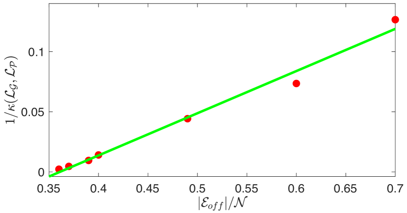
Figure 6. Condition number change with number of off-tree edges added for fe$\_$4elt graph

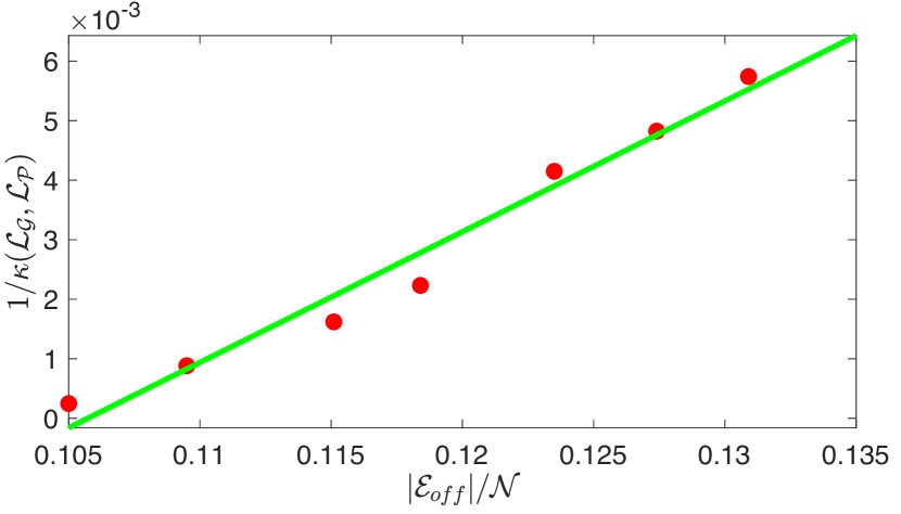
Figure 7. Condition number change with number of off-tree edges added for PPI graph

Figure 7 and Figure 7 show the changes of the relative condition numbers with increasing number of off-tree edges added to the initial spanning-tree sparsifier for PPI and fe$\_$4elt graphs. It can be observed that smaller condition number can be achieved with greater number of off-tree edges included, which indicates that very desired (flexible) tradeoffs between graph complexity and approximation quality can be obtained.

4.2. SF-GRASS for PCG Iterations

Table 3. Results of the PCG solver for SF-GRASS.

Test cases	$\mathcal{N}$	$\mathcal{M}$	directed solver	PCG for SF-GRASS				PCG for GRASS
				$T$	$\frac{|\mathcal{E}_{off}|}{\mathcal{N}}$	$iter$	$relres$	$T$	$\frac{|\mathcal{E}_{off}|}{\mathcal{N}}$	$iter$	$relres$
Thermal1	$2.5E4$	$7.2E4$	$1.12s$	$0.13s$	$2.7\%$	$3$	$5.6E-4$	$0.26s$	$2.6\%$	$7$	$4.5E-4$
Thermal2	$1.0E5$	$2.9E5$	$5.95s$	$0.79s$	$2.9\%$	$3$	$5.9E-4$	$3.31s$	$2.9\%$	$7$	$5.7E-4$
Thermal3	$2.0E5$	$5.9E5$	$19.42s$	$3.41s$	$3.2\%$	$4$	$1.8E-4$	$9.44s$	$2.9\%$	$8$	$6.3E-4$
Thermal4	$4.0E5$	$1.2E6$	$72.47s$	$8.01s$	$3.1\%$	$3$	$6.0E-4$	$63.52s$	$2.9\%$	$6$	$8.6E-4$
Thermal5	$9.0E5$	$2.6E6$	$974.87s$	$21.28s$	$3.1\%$	$3$	$6.2E-4$	$919.35s$	$3.0\%$	$6$	$8.2E-4$
Thermal6	$1.6E6$	$4.6E6$	$3637.79s$	$42.02s$	$3.1\%$	$3$	$6.1E-4$	$1695.92s$	$3.0\%$	$6$	$5.6E-4$
Thermal7	$2.0E6$	$5.9E6$	$2787.94s$	$69.62s$	$3.2\%$	$3$	$6.2E-4$	$7932.55s$	$3.0\%$	$6$	$6.2E-4$
Thermal8	$2.5E6$	$7.2E6$	$9341.48s$	$56.36s$	$3.2\%$	$3$	$6.1E-4$	$5476.88s$	$3.0\%$	$6$	$6.2E-4$

The spectral sparsifier generated by the proposed algorithm is leveraged as a preconditioner in a PCG solver for solving linear system equations $Ax=b$. The preconditioner matrix is factorized with Cholmod solver (cholmod, ). The right-hand-side (RHS) vector $b$ is generated randomly, while the solver is set to converge to an accuracy level $\|Ax-b\|/\|b\|<1E-3$ for all test cases. We compare the PCG solver using SF-GRASS with the direct method and the PCG solver using GRASS, as shown in Table 3. $T$ represents the total runtime for each solver, $iter$ represents the number of iterations, and $relres$ is the relative residue. It shows that SF-GRASS is the fastest among all three solvers, which can achieve up to $167X$ and $98X$ speedups when comparing to direct solver and PCG solver using GRASS, respectively. Also, SF-GRASS has achieved a faster convergence rate than GRASS.

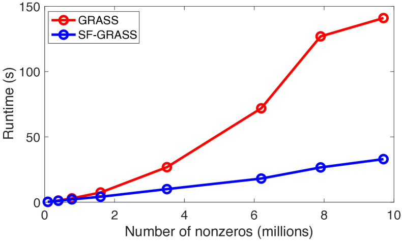
Figure 8. Runtime scalability comparison: GRASS vs SF-GRASS (3D meshes of different sizes)

Figure 8 shows the runtime scalability of GRASS and SF-GRASS on different sizes of 3D mesh graphs. It indicates that SF-GRASS scales linearly with the graph size, which is more scalable than GRASS, especially on larger and denser graphs, such as 3D mesh graphs.

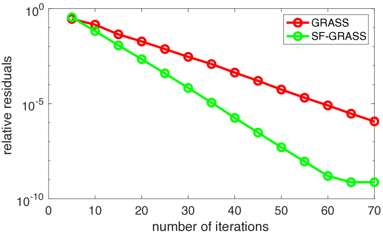
Figure 9. Convergence rate comparison for a 3D thermal grid: GRASS vs SF-GRASS

Figure 9 shows the convergence rate of PCG solver when using the sparsifiers generated by GRASS and SF-GRASS on a 3D thermal grid with $1.0E5$ nodes and $3.0E5$ edges. To generate the sparsifiers, we add ${0.018\mathcal{N}}$ off-tree edges to the sparsifiers for both SF-GRASS and GRASS settings. It shows that SF-GRASS has achieved a better convergence rate than GRASS.

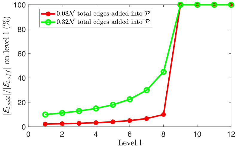
Figure 10. Edge sampling probabilities for each coarse-level graph of Thermal3, where total $0.08\mathcal{N}$ and $0.32\mathcal{N}$ number of edges are added into $\mathcal{P}$, respectively

Figure 10 shows the edge sampling probabilities on each coarse level graph of a 3D thermal mesh grid, where $0.08\mathcal{N}$ and $0.32\mathcal{N}$ off-tree edges have been added to the initial spanning-tree sparsifier $\mathcal{P}$ across all levels, respectively. $|\mathcal{E}_{l,add}|$ denotes the number of off-subgraph edges added on level $l$ graph, and $|\mathcal{E}_{l,off}|$ denotes the total off-subgraph edges on level $l$. As shown, the edges on coarser graphs have been assigned with higher sampling probabilities since they will have greater effective-resistances and thus be more important for retaining the original graph structural (spectral) properties.

4.3. SF-GRASS for Vectorless Verification

Table 4. Results of the proposed vectorless power grid integrity verification method.

	Power Grid Specs.			Single Level			Multilevel w/o Sparsifier				Multilevel w/ Sparsifer
$CKT$	$\mathcal{N}.\#$	$\mathcal{C}.\#$	${L}.\#$	$T_{chol}$	$T_{sol}$	$T_{lp}$	$T_{chol}$	$T_{sol}$	$T_{lp}$	$Err(\%)$	$T_{chol}$	$T_{sol}$	$T_{lp}$	$Err(\%)$	$\kappa$
$ibmpg3$	$8.5E5$	$9.0E4$	$2$	$11.91s$	$0.40s$	$1.63s$	$15.55s$	$0.51s$	$0.05s$	$1.76\%$	$1.70s$	$0.04s$	$0.03s$	$1.85\%$	$239$
$ibmpg4$	$1.0E6$	$1.0E5$	$2$	$14.97s$	$0.53s$	$1.67s$	$20.99s$	$0.73s$	$0.14s$	$2.71\%$	$1.68s$	$0.04s$	$0.10s$	$3.52\%$	$1136$
$ibmpg5$	$1.1E6$	$1.6E5$	$2$	$8.48s$	$0.27s$	$2.08s$	$12.58s$	$0.43s$	$0.22s$	$2.43\%$	$2.10s$	$0.05s$	$0.17s$	$2.52\%$	$218$
$ibmpg6$	$1.7E6$	$1.7E5$	$2$	$12.24s$	$0.36s$	$3.21s$	$17.76s$	$0.51s$	$0.20s$	$1.36\%$	$3.05s$	$0.07s$	$0.06s$	$3.83\%$	$248$
$thupg1$	$5.0E6$	$5.0E5$	$2$	$72.44s$	$2.07s$	$9.40s$	$290.36s$	$4.06s$	$28.31s$	$1.73\%$	$11.96s$	$0.25s$	$4.93s$	$3.31\%$	$464$
$thupg2$	$9.0E6$	$9.0E5$	$2$	$955.00s$	$4.53s$	$33.40s$	$1142.46s$	$6.59s$	$14.26s$	$4.20\%$	$52.75s$	$0.50s$	$9.90s$	$2.64\%$	$465$

We also evaluated SF-GRASS for vectorless power grid verifications using industrial power gird designs with different sizes (ibmpg, ), as shown in Table 4. The vectorless verification framework is adopted from (zhiqiang:dac17, ). “Single Level”, “Multilevel w/o Sparsifier”, and “Multilevel w/ Sparsifier” denote the verification methods using single level (direct), multilevel grids w/o sparsification and w/ sparsification using SF-GRASS, respectively. Note that we choose to apply sparsified power grid on each level generated by SF-GRASS during the verification process. $\mathcal{N}.\#$, $\mathcal{C}.\#$, ${L}.\#$ are the numbers of grid nodes, current sources, and hierarchical levels, respectively. $T_{chol}$, $T_{sol}$ and $T_{lp}$ denote the runtime for Cholesky factorizations, adjoint sensitivity calculation using matrix factors and the total LP solution time including all levels, respectively. $Err$ denotes the relative error of maximum voltage drop compared to the single-level method, and $\kappa$ denotes the relative condition number.

For all test cases, it is observed that matrix factorization, sensitivity calculation, and LP solving can be significantly accelerated using the SF-GRASS while maintaining excellent accuracy. The “Multilevel w/o Sparsifier” method is always the slowest due to the fast-growing matrix densities at coarse levels.

5. Conclusions

For the first time, we present a solver-free spectral graph sparsification approach (SF-GRASS) by leveraging emerging spectral graph coarsening and graph signal processing (GSP) techniques. Such a scalable framework allows constructing a hierarchy of spectrally-reduced and sparsified graphs in nearly-linear time, which can become key to accelerating many graph-based numerical computing tasks. The proposed spectral approach is simple to implement and inherently parallel friendly. Our extensive experimental results show that the proposed method can produce a hierarchy of high-quality spectral sparsifiers in nearly-linear time for a variety of real-world, large-scale graphs and circuit networks when compared with prior state-of-the-art spectral methods.

6. Acknowledgments

This work is supported in part by the National Science Foundation under Grants CCF-1350206 (CAREER), CCF-2021309 (SHF), and CCF-2011412 (SHF).

References

- [1] I. Abraham and O. Neiman. Using petal-decompositions to build a low stretch spanning tree. In Proceedings of the forty-fourth annual ACM symposium on Theory of computing (STOC), pages 395–406. ACM, 2012.
- [2] J. Batson, D. Spielman, and N. Srivastava. Twice-Ramanujan Sparsifiers. SIAM Journal on Computing, 41(6):1704–1721, 2012.
- [3] A. A. Benczúr and D. R. Karger. Approximating st minimum cuts in õ (n 2) time. In Proceedings of the twenty-eighth annual ACM symposium on Theory of computing (STOC), pages 47–55. ACM, 1996.
- [4] A. A. Benczúr and D. R. Karger. Randomized approximation schemes for cuts and flows in capacitated graphs. SIAM Journal on Computing, 44(2):290–319, 2015.
- [5] T. Davis. CHOLMOD: sparse supernodal Cholesky factorization and update/downdate. [Online]. Available: http://www.cise.ufl.edu/research/sparse/cholmod/, 2008.
- [6] C. Deng, Z. Zhao, Y. Wang, Z. Zhang, and Z. Feng. Graphzoom: A multi-level spectral approach for accurate and scalable graph embedding. International Conference on Learning Representations (ICLR), 2020.
- [7] M. Elkin, Y. Emek, D. A. Spielman, and S.-H. Teng. Lower-stretch spanning trees. SIAM Journal on Computing, 38(2):608–628, 2008.
- [8] Z. Feng. Spectral graph sparsification in nearly-linear time leveraging efficient spectral perturbation analysis. In Proceedings of the 53rd Annual Design Automation Conference, pages 1–6, 2016.
- [9] Z. Feng. Similarity-aware spectral sparsification by edge filtering. In Design Automation Conference (DAC), 2018 55nd ACM/EDAC/IEEE, pages 1–6. IEEE, 2018.
- [10] Z. Feng. Grass: Graph spectral sparsification leveraging scalable spectral perturbation analysis. IEEE Transactions on Computer-Aided Design of Integrated Circuits and Systems, 2020.
- [11] L. Han, X. Zhao, and Z. Feng. An Adaptive Graph Sparsification Approach to Scalable Harmonic Balance Analysis of Strongly Nonlinear Post-Layout RF Circuits. Computer-Aided Design of Integrated Circuits and Systems, IEEE Transactions on, 34(2):173–185, 2015.
- [12] C. Hong, A. Sukumaran-Rajam, B. Bandyopadhyay, J. Kim, S. E. Kurt, I. Nisa, S. Sabhlok, Ü. V. Çatalyürek, S. Parthasarathy, and P. Sadayappan. Efficient sparse-matrix multi-vector product on gpus. In Proceedings of the 27th International Symposium on High-Performance Parallel and Distributed Computing, pages 66–79. ACM, 2018.
- [13] J. A. Kelner, Y. T. Lee, L. Orecchia, and A. Sidford. An Almost-linear-time Algorithm for Approximate Max Flow in Undirected Graphs, and Its Multicommodity Generalizations. In Proceedings of the twenty-fifth annual ACM-SIAM symposium on Discrete algorithms, pages 217–226. SIAM, 2014.
- [14] T. N. Kipf and M. Welling. Semi-supervised classification with graph convolutional networks. arXiv e-print, arXiv:1609.02907, 2016.
- [15] J. R. Lee, S. O. Gharan, and L. Trevisan. Multiway spectral partitioning and higher-order cheeger inequalities. Journal of the ACM (JACM), 61(6):37, 2014.
- [16] Y. T. Lee and H. Sun. An SDP-based Algorithm for Linear-sized Spectral Sparsification. In Proceedings of the 49th Annual ACM SIGACT Symposium on Theory of Computing, STOC 2017, pages 678–687, New York, NY, USA, 2017. ACM.
- [17] O. Livne and A. Brandt. Lean algebraic multigrid (LAMG): Fast graph Laplacian linear solver. SIAM Journal on Scientific Computing, 34(4):B499–B522, 2012.
- [18] A. Loukas. Graph reduction with spectral and cut guarantees. Journal of Machine Learning Research, 20(116):1–42, 2019.
- [19] A. Loukas and P. Vandergheynst. Spectrally approximating large graphs with smaller graphs. In International Conference on Machine Learning, pages 3243–3252, 2018.
- [20] S. R. Nassif. IBM power grid benchmarks. [Online]. Available: http://dropzone.tamu.edu/ pli/PGBench/, 2008.
- [21] R. Peng. Algorithm Design Using Spectral Graph Theory. PhD thesis, Carnegie Mellon University, 2013.
- [22] R. Peng, H. Sun, and L. Zanetti. Partitioning well-clustered graphs: Spectral clustering works. In Proceedings of The 28th Conference on Learning Theory (COLT), pages 1423–1455, 2015.
- [23] D. I. Shuman, S. K. Narang, P. Frossard, A. Ortega, and P. Vandergheynst. The emerging field of signal processing on graphs: Extending high-dimensional data analysis to networks and other irregular domains. IEEE Signal Processing Magazine, 30(3):83–98, 2013.
- [24] D. Spielman and N. Srivastava. Graph sparsification by effective resistances. SIAM Journal on Computing, 40(6):1913–1926, 2011.
- [25] D. Spielman and S. Teng. Spectral sparsification of graphs. SIAM Journal on Computing, 40(4):981–1025, 2011.
- [26] D. Spielman and S. Teng. Nearly linear time algorithms for preconditioning and solving symmetric, diagonally dominant linear systems. SIAM Journal on Matrix Analysis and Applications, 35(3):835–885, 2014.
- [27] M. Steinberger, R. Zayer, and H.-P. Seidel. Globally homogeneous, locally adaptive sparse matrix-vector multiplication on the gpu. In Proceedings of the International Conference on Supercomputing, page 13. ACM, 2017.
- [28] S.-H. Teng. Scalable algorithms for data and network analysis. Foundations and Trends® in Theoretical Computer Science, 12(1–2):1–274, 2016.
- [29] X. Zhao, L. Han, and Z. Feng. A Performance-Guided Graph Sparsification Approach to Scalable and Robust SPICE-Accurate Integrated Circuit Simulations. Computer-Aided Design of Integrated Circuits and Systems, IEEE Transactions on, 34(10):1639–1651, 2015.
- [30] Z. Zhao and Z. Feng. A spectral graph sparsification approach to scalable vectorless power grid integrity verification. In Proceedings of the 54th Annual Design Automation Conference 2017, page 68. ACM, 2017.
- [31] Z. Zhao and Z. Feng. Effective-resistance preserving spectral reduction of graphs. In Proceedings of the 56th Annual Design Automation Conference (DAC) 2019, page 109. ACM, 2019.
- [32] Z. Zhao, Y. Wang, and Z. Feng. SAMG: Sparsified Graph Theoretic Algebraic Multigrid for Solving Large Symmetric Diagonally Dominant (SDD) Matrices. In Proceedings of the 36th International Conference on Computer-Aided Design (ICCAD). ACM, 2017.
- [33] Z. Zhao, Y. Wang, and Z. Feng. Nearly-linear time spectral graph reduction for scalable graph partitioning and data visualization. arXiv e-print, arXiv:1812.08942, 2018.