Bridging the Gap between Optimal Trajectory Planning and Safety-Critical Control with Applications to Autonomous Vehicles

Abstract

We address the problem of optimizing the performance of a dynamic system while satisfying hard safety constraints at all times. Implementing an optimal control solution is limited by the computational cost required to derive it in real time, especially when constraints become active, as well as the need to rely on simple linear dynamics, simple objective functions, and ignoring noise. The recently proposed Control Barrier Function (CBF) method may be used for safety-critical control at the expense of sub-optimal performance. In this paper, we develop a real-time control framework that combines optimal trajectories generated through optimal control with the computationally efficient CBF method providing safety guarantees. We use Hamiltonian analysis to obtain a tractable optimal solution for a linear or linearized system, then employ High Order CBFs (HOCBFs) and Control Lyapunov Functions (CLFs) to account for constraints with arbitrary relative degrees and to track the optimal state, respectively. We further show how to deal with noise in arbitrary relative degree systems. The proposed framework is then applied to the optimal traffic merging problem for Connected and Automated Vehicles (CAVs) where the objective is to jointly minimize the travel time and energy consumption of each CAV subject to speed, acceleration, and speed-dependent safety constraints. In addition, when considering more complex objective functions, nonlinear dynamics and passenger comfort requirements for which analytical optimal control solutions are unavailable, we adapt the HOCBF method to such problems. Simulation examples are included to compare the performance of the proposed framework to optimal solutions (when available) and to a baseline provided by human-driven vehicles with results showing significant improvements in all metrics.

1 INTRODUCTION

Optimizing a cost function associated with the operation of a dynamical system while also satisfying hard safety constraints at all times is a fundamental and challenging problem. The challenge is even greater when stabilizing some system state variables to desired values is an additional requirement. With the growing role of autonomy, the importance of these problems has also grown and one now frequently encounters them in the operation of autonomous vehicles in robotics and traffic networks. These applications provide the main motivation for the control framework presented in this paper.

Optimal control problems with safety-critical constraints can be solved through standard methods Bryson and Ho (1969), Ansari and Murphey (2016), with applications found in robotics and autonomous vehicles in traffic networks Chitour et al. (2012), Mita et al. (2001), Malikopoulos et al. (2018), Xiao and Cassandras (2019a). However, analytical solutions are only possible for simple system dynamics and constraints. Moreover, the computational complexity for deriving such solutions significantly increases as one or more constraints become active and it grows as a power function of the number of constraints. This fact limits the use of optimal control methods for autonomous systems when solutions need to be derived and executed on line. Additional factors which further limit the real-time use of these methods include the presence of noise in the dynamics, model inaccuracies, environmental perturbations, and communication delays in the information exchange among system components. Thus, there is a gap between optimal control solutions (which represent a lower bound for the optimal achievable cost) and the execution of controllers aiming to achieve such solutions under realistic operational conditions.

In order to bridge this gap and obtain real-time controls for safety-critical problems, Model Predictive Control (MPC) Garcia and Prett (1989), Mayne (2014), Bemporad et al. (2002) has been widely used to approximate optimal control solutions. Whether linear or nonlinear MPC methods are used, a time-discretized predictive model is needed and a receding horizon control problem is formulated and solved at all discretized receding time instants taking into account all safety constraints involved. Nonetheless, the computational cost significantly increases with the model nonlinearity and the time horizon over which a problem is solved.

An alternative approach which has the potential to avoid the drawbacks above is based on the use of Control Barrier Function (CBFs). Barrier functions are Lyapunov-like functions Wieland and Allgower (2007) whose use can be traced back to optimization theory Boyd and Vandenberghe (2004). More recently, they have been employed in verification and control, e.g., to prove set invariance Aubin (2009), Prajna et al. (2007), Wisniewski and Sloth (2013), and for multi-objective control Panagou et al. (2013). CBFs are extensions of barrier functions for control systems Ames et al. (2017) and have been recently generalized to consider arbitrary relative degree constraints in Nguyen and Sreenath (2016), Xiao and Belta (2019). It has also been shown that CBFs can be combined with Control Lyapunov Functions (CLFs) Sontag (1983), Freeman and Kokotovic (1996), Ames et al. (2012) to form constrained quadratic programs (QPs) Galloway et al. (2015) for nonlinear control systems that are affine in controls. The main advantages of CBF-based control compared to MPC lie in the fact that $(i)$ feasible state sets under CBF-based control possess a forward invariance guarantee property, $(ii)$ The QPs involved at every time step can be solved in real time, as long as each QP is feasible, and $(iii)$ the method is easier to adapt when handling nonlinear systems with complex constraints.

The contribution of this paper is to synthesize controllers that combine the optimal control and the CBF methods aiming for both optimality and guaranteed safety in real-time control. The key idea is to first generate trajectories by solving a tractable optimal control problem and then seek to track these trajectories using a controller which simultaneously ensures that all state and control constraints are satisfied at all times. This is accomplished in two steps. The first step is to solve a constrained optimal control problem. Given a set of initial conditions, it is usually possible to derive simple conditions under which it can be shown that no constraint becomes active. In this case, executing the unconstrained optimal control solution becomes a relatively simple tracking problem. Otherwise, we can still often derive an optimal control solution consisting of both unconstrained and constrained arcs. However, such derivations may not always be feasible in real time. Either way, using the best possible analytical solution within reasonable real-time computational constraints (possibly just the unconstrained solution), this step leads to a reference control $u_{ref}(t)$, $t\in[0,T]$. The second step is then to use High Order CBFs (HOCBFs) Xiao and Belta (2019) to account for constraints with arbitrary relative degrees, and define a sequence of QPs whose goal is to optimally track $u_{ref}(t)$ at each discrete time step over $[0,T]$. In this step, we can allow noise in the system dynamics and include nonlinearities which were ignored in the original optimal control solution. The resulting controller is termed Optimal control with Control Barrier Functions (OCBF). We will show that using an OCBF controller we can achieve near-optimal performance relative to the one under optimal control while guaranteeing constraint satisfaction under more general dynamics and the presence of disturbances that the original optimal control solution cannot capture.

The OCBF idea was used in our recent work Xiao et al. (2019b) to address the merging problem for Connected Automated Vehicles (CAVs) in traffic networks. This is one of the most challenging problems within a transportation system in terms of safety, congestion, and energy consumption, in addition to being a source of stress for many drivers Schrank et al. (2015), Tideman et al. (2007), Waard et al. (2009). More broadly, advances in transportation system technologies and the emergence of CAVs have the potential to drastically improve a transportation network’s performance by better assisting drivers in making decisions, ultimately reducing energy consumption, air pollution, congestion and accidents. Early efforts exploiting the benefit of CAVs were proposed in Levine and Athans (1966), Varaiya (1993). In terms of optimal trajectory planning, a number of centralized and decentralized merging control mechanisms have been proposed Milanes et al. (2012), Tideman et al. (2007), Raravi et al. (2007), Scarinci and Heydecker (2014). In the case of decentralized control, all computation is performed on board each vehicle and shared only with a small number of other vehicles which are affected by it. The objectives specified for optimal control problems may target the minimization of acceleration as in Rios-Torres and Malikopoulos (2017) or the maximization of passenger comfort (measured as the acceleration derivative or jerk) as in Ntousakis et al. (2016), Rathgeber et al. (2015). MPC techniques are employed as an alternative, primarily to account for additional constraints and to compensate for disturbances by re-evaluating optimal actions Cao et al. (2015), Mukai et al. (2017), Ntousakis et al. (2016). As an alternative to MPC, CBF methods were used in Xiao et al. (2019a) where a decentralized optimal control problem with explicit analytical solutions for each CAV was derived.

In this paper, we generalize the OCBF controller introduced in Xiao et al. (2019b) that only works for relative degree one constraints to allow constraints with relative degree greater than one and also allow for noise in the system dynamics. We consider optimal control problems with constraints of arbitrary relative degrees which are handled by using HOCBFs. We will show that by using HOCBFs we can incorporate complex objective functions, nonlinear dynamics, and comfort requirements which otherwise prohibit even unconstrained optimal control solutions from being derived. This also allows us to study the trade-off between travel time, energy consumption, and comfort. Extensive simulations have been conducted to demonstrate the effectiveness of the proposed framework for the traffic merging problem relative to other approaches.

The paper is structured as follows. In Section 2, we provide definitions and results on the HOCBF method. We formulate a general constrained optimal control problem and develop its OCBF solution in Sections 3 and 4, respectively. As an application of the OCBF framework, in Section 5 we present the traffic merging process model and formulate the optimal merging control problem including all safety, state and control constraints that must be satisfied at all times. In Section 6, the optimal solution for the merging problem is reviewed for the unconstrained as well as the constrained cases and the OCBF method is applied to it. We provide simulation examples and performance comparisons with human-driven vehicles in Section 7 and conclude with Section 8.

2 PRELIMINARIES

Consider an affine control system of the form

$$\dot{\bm{x}}=f(\bm{x})+g(\bm{x})\bm{u}$$ (1)

where $\bm{x}\in X\subset\mathbb{R}^{n}$, $f:\mathbb{R}^{n}\rightarrow\mathbb{R}^{n}$ and $g:\mathbb{R}^{n}\rightarrow\mathbb{R}^{n\times q}$ are globally Lipschitz, and $\bm{u}\in U\subset\mathbb{R}^{q}$ ($U$ denotes the control constraint set). Solutions $\bm{x}(t)$ of (1), starting at $\bm{x}(0)$, $t\geq 0$, are forward complete. The control constraint set $U$ is defined as (the inequality is interpreted componentwise, $\bm{u}_{min},\bm{u}_{max}\in\mathbb{R}^{q}$):

$$U:=\{\bm{u}\in\mathbb{R}^{q}:\bm{u}_{min}\leq\bm{u}\leq\bm{u}_{max}\}.$$ (2)

Definition 1

(Class $\mathcal{K}$ function Khalil (2002)) A continuous function $\alpha:[0,a)\rightarrow[0,\infty),a>0$ is said to belong to class $\mathcal{K}$ if it is strictly increasing and $\alpha(0)=0$.

Definition 2

A set $C\subset\mathbb{R}^{n}$ is forward invariant for system (1) if its solutions starting at any $\bm{x}(0)\in C$ satisfy $\bm{x}(t)\in C,\forall t\geq 0$.

Definition 3

(Relative degree) The relative degree of a (sufficiently many times) differentiable function $b:\mathbb{R}^{n}\rightarrow\mathbb{R}$ with respect to system (1) is the number of times it is differentiated along the dynamics (1) until the control $\bm{u}$ explicitly shows in the corresponding derivative.

In this paper, the function $b$ is used to define a constraint $b(\bm{x})\geq 0$. Therefore, we will also refer to the relative degree of $b$ as the relative degree of the constraint. For a constraint $b(\bm{x})\geq 0$ with relative degree $m$, $b:\mathbb{R}^{n}\rightarrow\mathbb{R}$, and $\psi_{0}(\bm{x}):=b(\bm{x})$, we define a sequence of functions $\psi_{i}:\mathbb{R}^{n}\rightarrow\mathbb{R},i\in\{1,\dots,m\}$:

$$\psi_{i}(\bm{x}):=\dot{\psi}_{i-1}(\bm{x})+\alpha_{i}(\psi_{i-1}(\bm{x})),\;\;\;i\in\{1,\dots,m\},$$ (3)

where $\alpha_{i}(\cdot),i\in\{1,\dots,m\}$ denotes a $(m-i)^{th}$ order differentiable class $\mathcal{K}$ function. We further define a sequence of sets $C_{i},i\in\{1,\dots,m\}$ associated with (3) in the form:

$$C_{i}:=\{\bm{x}\in\mathbb{R}^{n}:\psi_{i-1}(\bm{x})\geq 0\},\;\;\;i\in\{1,\dots,m\}.$$ (4)

Definition 4

(High Order Control Barrier Function (HOCBF) Xiao and Belta (2019)) Let $C_{1},\dots,C_{m}$ be defined by (4) and $\psi_{1}(\bm{x}),\dots,\psi_{m}(\bm{x})$ be defined by (3). A function $b:\mathbb{R}^{n}\rightarrow\mathbb{R}$ is a high order control barrier function (HOCBF) of relative degree $m$ for system (1) if there exist $(m-i)^{th}$ order differentiable class $\mathcal{K}$ functions $\alpha_{i},i\in\{1,\dots,m-1\}$ and a class $\mathcal{K}$ function $\alpha_{m}$ such that

$$\sup_{\bm{u}\in U}[L_{f}^{m}b(\bm{x})\!+\!L_{g}L_{f}^{m-1}b(\bm{x})\bm{u}\!+\!S(b(\bm{x}))\!+\!\alpha_{m}(\psi_{m-1}(\bm{x}))]\geq 0$$ (5)

for all $\bm{x}\in C_{1}\cap,\dots,\cap C_{m}$. In (5), $L_{f}^{m}$ ($L_{g}$) denotes Lie derivatives along $f$ ($g$) $m$ (one) times, and $S(\cdot)$ denotes the remaining Lie derivatives along $f$ with degree less than or equal to $m-1$.

The HOCBF constraints in (5) may sometimes conflict with the control constraints in (2), which can limit the existence of feasible solutions for the optimal control problem that we will formulate later. In order to minimize this effect, the penalty method Xiao and Belta (2019) replaces $\alpha_{i}(\psi_{i-1}(\bm{x}))$ by $p_{i}\cdot\alpha_{i}(\psi_{i-1}(\bm{x})),\forall i\in\{1,\dots,m\}$, where $p_{i}>0$ is a multiplicative penalty factor which can be tuned appropriately.

Theorem 1

(Xiao and Belta (2019)) Given a HOCBF $b(\bm{x})$ from Def. 4 with the associated sets $C_{1},\dots,C_{m}$ defined by (4), if $\bm{x}(0)\in C_{1}\cap,\dots,\cap C_{m}$, then any Lipschitz continuous controller $\bm{u}(t)\in U$ that satisfies (5), $\forall t\geq 0$ renders $C_{1}\cap,\dots,\cap C_{m}$ forward invariant for system (1).

The HOCBF is a general form of the relative degree one CBF Ames et al. (2017), Glotfelter et al. (2017) (i.e., setting $m=1$ reduces the HOCBF to the common CBF form in Ames et al. (2017), Glotfelter et al. (2017)). The exponential CBF Nguyen and Sreenath (2016) is a special case of the HOCBF.

Definition 5

(Control Lyapunov function (CLF) Ames et al. (2012)) A continuously differentiable function $V:\mathbb{R}^{n}\rightarrow\mathbb{R}$ is a globally and exponentially stabilizing control Lyapunov function (CLF) for system (1) if there exist constants $c_{1}>0,c_{2}>0,c_{3}>0$ such that

$$c_{1}||\bm{x}||^{2}\leq V(\bm{x})\leq c_{2}||\bm{x}||^{2}$$ (6)

$$\inf_{u\in U}[L_{f}V(\bm{x})+L_{g}V(\bm{x})\bm{u}+c_{3}V(\bm{x})]\leq 0.$$ (7)

for $\forall\bm{x}\in\mathbb{R}^{n}$.

Theorem 2

(Ames et al. (2012)) Given an exponentially stabilizing CLF $V$ as in Def. 5, any Lipschitz continuous controller $\bm{u}(t)\in U$ that satisfies (7), $\forall t\geq 0$ exponentially stabilizes system (1) to the origin.

Note that (7) can be relaxed by replacing $0$ by a relaxation variable $\delta\geq 0$ at its right-hand side which can be subsequently minimized Ames et al. (2012).

Many existing works Ames et al. (2017),Lindemann and Dimarogonas (2019),Nguyen and Sreenath (2016) combine CBFs for systems with relative degree one with quadratic costs to form optimization problems. Time is discretized and an optimization problem with constraints given by the CBFs (inequalities of the form (5)) is solved at each time step. If convergence to a state is desired, then a CLF constraint of the form (7) is added. Note that these constraints are linear in control since the state value is fixed at the beginning of the interval, therefore, each optimization problem is a quadratic program (QP). The optimal control obtained by solving each QP is applied at the current time step and held constant for the whole interval. The state is updated using dynamics (1), and the procedure is repeated. Replacing CBFs by HOCBFs allows us to handle constraints with arbitrary relative degree Xiao and Belta (2019).

3 PROBLEM FORMULATION AND APPROACH

$\mathbf{Objective}$: (Cost minimization) Consider an optimal control problem for system (1) with the cost defined as:

$$J=\int_{t_{0}}^{t_{f}}\left[\beta+\mathcal{C}(\bm{x},\bm{u},t)\right]dt,$$ (8)

where $t_{0},t_{f}$ denote the initial and final times, respectively, and $\mathcal{C}:\mathbb{R}^{n}\times\mathbb{R}^{q}\times[t_{0},t_{f}]\rightarrow\mathbb{R}^{+}$ is a cost function. The parameter $\beta\geq 0$ is used to capture a trade-off between the minimization of the time interval $(t_{f}-t_{0})$ and the operational cost $\mathcal{C}(\bm{x},\bm{u},t)$. The terminal time $t_{f}$ is constrained as follows:

Terminal state constraint: The state of system (1) is constrained to reach a point $\bar{\bm{X}}\in{X}$, i.e.,

$$\bm{x}(t_{f})=\bar{\bm{X}},$$ (9)

Note that $t_{f}$ is generally free (unspecified).

Constraint 1 (Safety constraints): Let $S_{o}$ denote an index set for a set of safety constraints. System (1) should always satisfy

$$b_{j}(\bm{x}(t))\geq 0,\text{ \ }\forall t\in[t_{0},t_{f}].$$ (10)

where each $b_{j}:\mathbb{R}^{n}\rightarrow\mathbb{R},j\in S_{o}$ is continuously differentiable.

Constraint 2 (Control constraints): These are provided by the control constraint set in (2).

Constraint 3 (State constraints): System (1) should always satisfy the state constraints (componentwise):

$$\bm{x}_{\min}\leq\bm{x}(t)\leq\bm{x}_{\max},\forall t\in[t_{0},t_{f}]$$ (11)

where $\bm{x}_{\min}\in\mathbb{R}^{n}$ and $\bm{x}_{\max}\in\mathbb{R}^{n}$. Note that we distinguish the state constraints from the safety constraints in (10) since the latter are viewed as hard, while the former usually capture system capability limitations that can be relaxed to improve the problem feasibility; for example, in traffic networks vehicles are constrained by upper and lower speed limits.

Problem 1

Find a control policy for system (1) such that the cost (8) is minimized, constraints (10),(11) and (2) are strictly satisfied, and deviations $||\bm{x}(t_{f})-\bar{\bm{X}}||^{2}$ from the terminal state constraint (9) are minimized.

The cost in (8) can be properly normalized by defining $\beta:=\frac{\alpha\sup_{\bm{x}\in X,\bm{u}\in U,\tau\in[t_{0},t_{f}]}\mathcal{C}(\bm{x},\bm{u},\tau)}{(1-\alpha)}$ where $\alpha\in[0,1)$ and then multiplying (8) by $\frac{\alpha}{\beta}$. Thus, we construct a convex combination as follows:

$$\begin{aligned} J=\int_{t_{0}}^{t_{f}}\left(\alpha+\frac{(1-\alpha)\mathcal{C}(\bm{x},\bm{u},t)}{\sup_{\bm{x}\in X,\bm{u}\in U,\tau\in[t_{0},t_{f}]}\mathcal{C}(\bm{x},\bm{u},\tau)}\right)dt\end{aligned}.$$ (12)

If $\alpha=1$, then we solve (8) as a minimum time problem. The normalized cost (12) facilitates a trade-off analysis between the two metrics. However, we will use the simpler cost expression (8) throughout this paper. Thus, we can take $\beta\geq 0$ as a weight factor that can be adjusted to penalize time relative to the cost $\mathcal{C}(\bm{x},\bm{u},t)$ in (8).

Approach: Step 1: We use Hamiltonian analysis to obtain an optimal control $\bm{u}^{\ast}(t)$ and optimal state $\bm{x}^{\ast}(t)$, $t\in[t_{0},{t}_{f}]$ for the cost (8) and system (1), under the terminal state constraint (9), the safety constraints (10), and the control and state constraints (2), (11). In order to get an analytical optimal solution, we may linearize or simplify the dynamics (1).

Step 2: There are usually unmodelled dynamics and measurement noise in (1). Thus, we consider a modified version of system (1) to denote the real dynamics:

$$\dot{\bm{x}}=f(\bm{x})+g(\bm{x})\bm{u}+\bm{w},$$ (13)

where $\bm{w}\in\mathbb{R}^{n}$ denotes a vector of random processes in an appropriate probability space intended to capture disturbances for which a precise model is generally unknown. We consider $\bm{x}$ as a measured state which includes the effects of such unmodelled dynamics and measurement noise and which can be used in what follows. Allowing for the noisy dynamics (13), we set $\bm{u}_{ref}(t)=\bm{u}^{\ast}(t)$ (more generally, $\bm{u}_{ref}(t)=h(\bm{u}^{\ast}(t),\bm{x}^{\ast}(t),\bm{x}(t)),h:\mathbb{R}^{q}\times\mathbb{R}^{n}\times\mathbb{R}^{n}\rightarrow\mathbb{R}^{q}$) and use the HOCBF method to track the optimal control as a reference, i.e.,

$$\min_{\bm{u}(t)}\int_{t_{0}}^{t_{f}}||\bm{u}(t)-\bm{u}_{ref}(t)||^{2}dt$$ (14)

subject to $(i)$ the HOCBF constraints (5) corresponding to the safety constraints (10), $(ii)$ the state constraints (11), and $(iii)$ the control constraints (2). In order to better track the optimal state $\bm{x}^{\ast}(t)$ and minimize the deviation $||\bm{x}(t_{f})-\bar{\bm{X}}||^{2}$ from the terminal state constraint, we define a CLF $V(\bm{x}-\bm{x}^{\ast})$. Thus, the cost (14) is also subject to the corresponding CLF constraint (7). The resulting problem can then be solved by the approach described at the end of Sec. 2.

4 FROM PLANNING TO EXECUTION

In this section, we describe how to solve Problem 1 combining optimality with safety guarantees.

4.1 Optimal Trajectory Planning

Let us consider a properly linearized version of (13) without the noise $\bm{w}$:

$$\dot{\bm{x}}=A\bm{x}+B\bm{u},$$ (15)

where $\bm{x}=(x_{1},\dots,x_{n}),\bm{u}=(u_{1},\dots,u_{q}),A\in\mathbb{R}^{n\times n},B\in\mathbb{R}^{n\times q}$.

Let $\bm{\lambda}(t)$ be the costate vector corresponding to the state $\bm{x}$ in (15) and $\bm{b}(\bm{x})$ denote the vector obtained by concatenating all $b_{j}(\bm{x}),j\in S_{o}$. The Hamiltonian with the state constraints, control constraints and safety constraints adjoined (omitting time arguments for simplicity) is

$$H(\bm{x},\bm{\lambda},\bm{u})=\mathcal{C}(\bm{x},\bm{u},t)+\bm{\lambda}^{T}(A\bm{x}+B\bm{u})+\bm{\mu}_{a}^{T}(\bm{u}-\bm{u}_{\max})$$ (16)

$$+\bm{\mu}_{b}^{T}(\bm{u}_{\min}-\bm{u})+\bm{\mu}_{c}^{T}(\bm{x}-\bm{x}_{\max})+\bm{\mu}_{d}^{T}(\bm{x}_{\min}-\bm{x})$$

$$-\bm{\mu}_{e}^{T}\bm{b}(\bm{x})+\beta$$

The components of the Lagrange multiplier vectors $\bm{\mu}_{a},\bm{\mu}_{b},\bm{\mu}_{c},\bm{\mu}_{d},\bm{\mu}_{e}$ are positive when the constraints are active and become 0 when the constraints are strict.

First, we assume all the constraints (2), (10), (11) are not active in the time interval $[t_{0},t_{f}]$. The Hamiltonian (16) then reduces to

$$H(\bm{x},\bm{\lambda},\bm{u})=\mathcal{C}(\bm{x},\bm{u},t)+\bm{\lambda}^{T}(A\bm{x}+B\bm{u})+\beta$$ (17)

Observing that the terminal constraints (9) $\bm{\psi}:=\bm{x}-\bar{\bm{X}}=0$ are not explicit functions of time, the transversality condition Bryson and Ho (1969) is

$$\left.H(\bm{x}(t),\bm{\lambda}(t),\bm{u}(t))\right|_{t=t_{f}}=0$$ (18)

with $\bm{\lambda}(t_{f})=[(\bm{\nu}^{T}\frac{\partial\bm{\psi}}{\partial\bm{x}})^{T}]_{t=t_{f}}$ as the costate boundary condition, where $\bm{\nu}$ denotes a vector of Lagrange multipliers. The Euler-Lagrange equations become:

$$\dot{\bm{\lambda}}=-\frac{\partial H}{\partial\bm{x}}=-\frac{\partial C(\bm{x},\bm{u},t)}{\partial\bm{x}}-A^{T}\bm{\lambda},$$ (19)

and the necessary condition for optimality is

$$\frac{\partial H}{\partial\bm{u}}=\frac{\partial C(\bm{x},\bm{u},t)}{\partial\bm{u}}+B^{T}\bm{\lambda}=0.$$ (20)

With (17)-(20), the initial state of system (13), and the terminal constraint $\bm{x}(t_{f})=\bar{\bm{X}}$, we can derive an unconstrained optimal state trajectory $\bm{x}^{\ast}(t)$ and optimal control $\bm{u}^{\ast}(t)$, $t\in[t_{0},t_{f}]$, for Problem 1.

When one or more constraints in (2), (10), (11) become active in the time interval $[t_{0},t_{f}]$, we use the interior point analysis Bryson and Ho (1969) to determine the conditions that must hold on a constrained arc entry point and exit point (if one exists prior to $t_{f}$). We can then determine the optimal entry and exit points, as well as the constrained optimal control $\bm{u}^{\ast}(t)$ and optimal state trajectory $\bm{x}^{\ast}(t)$, $t\in[t_{0},t_{f}]$. Depending on the computational complexity involved in deriving the complete constrained optimal solution, we can specify a planned reference control $\bm{u}_{ref}(t)$ and state trajectory $\bm{x}_{ref}(t)$, $t\in[t_{0},t_{f}]$. For example, we may just plan for a safety-constrained solution and omit the state and control constraints (2), (11), or even plan for only the unconstrained optimal solution to simplify the trajectory planning process.

4.2 Safety-Critical Optimal Control with HOCBFs

We now introduce a method that tracks the planned optimal control and state trajectory while guaranteeing the satisfaction of all constraints (2), (10), (11) in Problem 1.

As detailed in Sec. 4.1, we use $\bm{u}^{\ast}(t)$ and $\bm{x}^{\ast}(t)$, $t\in[t_{0},t_{f}]$, to denote the optimal control and state trajectory derived under no active constraints or with some (or all) of the constraints active, depending on the associated computational complexity considered acceptable in a particular setting. We can then reformulate (8) as the following optimization problem:

$$\min_{\bm{u}(t)}\int_{t_{0}}^{t_{f}}||\bm{u}(t)-\bm{u}_{ref}(t)||^{2}dt$$ (21)

subject to (2), (10), (11), where

$$\bm{u}_{ref}(t)=F_{U}(\bm{u}^{\ast}(t),\bm{x}^{\ast}(t),\bm{x}(t))$$ (22)

is a specific function of the optimal control and state trajectory, as well as the actual state under noise $\bm{w}$ from (13). A typical choice for $F_{U}(\bm{u}^{\ast}(t),\bm{x}^{\ast}(t),\bm{x}(t))$ is

$$\bm{u}_{ref}(t)=e^{\sum_{j=1}^{n}\frac{x_{j}^{\ast}(t)-x_{j}(t)}{\sigma_{j}}}\bm{u}^{\ast}(t),$$ (23)

where $x_{j}(t),$ $j\in\{1,\dots,n\}$ denote the observed state variables under noise $\bm{w}$ from (13), $x_{j}^{\ast}(t),$ $j\in\{1,\dots,n\},$ $u_{i}^{\ast}(t),$ $i\in\{1,\dots,q\}$ denote the optimal state and control from the last subsection, and $\sigma_{j}>0,$ $j\in\{1,\dots,n\}$ are weight parameters. In (23), the sign of the term $x_{j}^{\ast}(t)-x_{j}(t)$ depends on whether $x_{j}(t)$ is increasing with $u_{i}(t)$. In particular, when $x_{j}(t)>x_{j}^{\ast}(t),$ for all $j\in\{1,\dots,n\}$, we have $u_{i}(t)<u_{i}^{\ast}(t)$ and the state errors can be automatically eliminated. If $x_{j}(t)<x_{j}^{\ast}(t),$ for all $j\in\{1,\dots,n\}$, the state errors can similarly be automatically eliminated. However, when $x_{j}(t)>x_{j}^{\ast}(t)$ and $x_{j+1}(t)<x_{j+1}^{\ast}(t)$, we may wish to enforce $u_{i}(t)<u_{i}^{\ast}(t),i\in\{1,\dots,q\}$. Thus, it is desirable that $\sigma_{j}<\sigma_{j+1}$ (similarly, when $x_{j}(t)<x_{j}^{\ast}(t)$ and $x_{j+1}(t)>x_{j+1}^{\ast}(t)$). In summary, we select $\sigma_{j}>0,$ $j\in\{1,\dots,n\}$ such that $\sigma_{j}<\sigma_{j+1},$ $j\in\{1,\dots,n-1\}$.

Alternative forms of (22) include

$$\bm{u}_{ref}(t)=\sum_{j\in\{1,\dots,n\}}\frac{x_{j}^{\ast}(t)}{x_{j}(t)}\bm{u}^{\ast}(t)$$ (24)

and the state feedback tracking control approach from Khalil (2002):

$$\bm{u}_{ref}(t)=\bm{u}^{\ast}(t)+\sum_{j=1}^{n}k_{j}(x_{j}^{\ast}(t)-x_{j}(t)),$$ (25)

where $k_{j}>0,\in\{1,\dots,n\}$. Clearly, there are several possible choices for the form of $\bm{u}_{ref}(t)$ which may depend on the specific application of interest.

We emphasize that the cost (21) is subject to all the constraints (2), (10), (11). We use HOCBFs to implement these constraints, as well as CLFs to better track the optimal state $\bm{x}^{\ast}(t)$, as shown in the following subsections.

4.2.1 Optimal State Tracking

First, we aim to track the optimal state $\bm{x}^{\ast}(t)$ obtained in Sec. 4.1 using CLFs. We can always find a state variable $x_{k},$ $k\in\{1,\dots,n\}$ in $\bm{x}$ that has relative degree one (assume $x_{k}$ is the output) with respect to system (13). This is because we only take the Lie derivative of the Lyapunov function once in the CLF constraint (7). Then, we define a controller aiming to drive $x_{k}(t)$ to $x_{ref}(t)$ where $x_{ref}(t)$ is of the form

$$x_{ref}(t)=F_{X}(\bm{x}^{\ast}(t),\bm{x}(t))$$ (26)

A typical choice analogous to (23) is

$$x_{ref}(t)=e^{\sum_{j\in\{1,\dots,n\}\setminus k}\frac{x_{j}^{\ast}(t)-x_{j}(t)}{\sigma_{j}}}x_{k}^{\ast}(t)$$ (27)

where $\sigma_{j}>0,$ $j\in\{1,\dots,n\}\setminus k$ and $\{1,\dots,n\}\setminus k$ denotes excluding $k$ from the set $\{1,\dots,n\}$. An alternative form analogous to (24) is

$$x_{ref}(t)=\sum_{j\in\{1,\dots,n\}\setminus k}\frac{x_{j}^{\ast}(t)}{x_{j}(t)}x_{k}^{\ast}(t)$$ (28)

where $x_{j}^{\ast}(t),$ $j\in\{1,\dots,n\}\setminus k$ are the (unconstrained or constrained) optimal state trajectories from the Section 4.1. In (28), if $x_{j}(t)>x_{j}^{\ast}(t)$, then $x_{ref}(t)<x_{k}^{\ast}(t)$, thus automatically reducing (or eliminating) the tracking error. Note that while $x_{ref}(t)$ in (28) depends heavily on the exact value of $x_{j}(t)$, an advantage of (27) is that it allows $x_{ref}(t)$ to depend only on the error. Clearly, we can define different tracking forms instead of (28) and (27) depending on the specific characteristics of an application.

Using a specific selected form of $x_{ref}(t)$, we can now proceed as in Def. 5 and define an output $y_{k}(t):=x_{k}(t)-x_{ref}(t)$ for the state variable $x_{k}$ which has relative degree one. Accordingly, we define a CLF $V(y_{k}(t))=y_{k}^{2}(t)$ with $c_{1}=c_{2}=1,c_{3}=\epsilon>0$ as in Def. 5. Then, any control input $\bm{u}(t)$ should satisfy, for all $t\in[t_{0},t_{f}]$,

$$L_{f}V(y_{k}(t))+L_{g}V(y_{k}(t))\bm{u}(t)+\epsilon V(y_{k}(t))\leq\delta_{k}(t)$$ (29)

where $\delta_{k}(t)$ is a relaxation variable (to be minimized as explained in the sequel) enabling the treatment of the requirement $x_{k}(t)=x_{ref}(t)$ as a soft constraint. Note that we may also identify other state variables with relative degree one and define multiple CLFs to better track the optimal state. Note that (29) does not include any (unknown) noise term. Also note that selecting a larger $\epsilon$ can improve the state convergence rate Ames et al. (2012).

4.2.2 Safety Constraints and State Limitations

Next, we use HOCBFs to map the safety constraints (10) and state limitations (11) from the state $\bm{x}(t)$ to the control input $\bm{u}(t)$. Let $b_{j}(\bm{x}),$ $j\in S_{o}$, be the HOCBF corresponding to the $j$th safety constraint. In addition, let $b_{i,\max}(\bm{x})=x_{i,\max}-x_{i}$ and $b_{i,\min}(\bm{x})=x_{i}-x_{i,\min},$ $i\in\{1,\dots,n\},$ be the HOCBFs for all state limitations, where $\bm{x}_{\max}=(x_{1,\max},\dots,x_{n,\max}),$ $\bm{x}_{\min}=(x_{1,\min},\dots,x_{n,\min})$. The relative degrees of $b_{i,\max}(\bm{x}),$ $b_{i,\min}(\bm{x}),$ $i\in\{1,\dots,n\}$ are $m_{i}$, and the relative degrees of $b_{j}(\bm{x}),$ $j\in S_{o}$ are $m_{j}$. Therefore, in Definition 4, we choose HOCBFs with $m=m_{i}$ or $m_{j}$, including the penalty factors $p_{i,\min}>0,p_{i,\max}>0,p_{i,safe}>0$ (see discussion after Definition 4) for all the class $\mathcal{K}$ functions. Following (5), any control input $u_{i}(t)$ should satisfy

$$L_{f}^{m_{j}}b_{j}(\bm{x})\!+\!L_{g}L_{f}^{m_{j}-1}b_{j}(\bm{x})\bm{u}\!+\!S(b_{j}(\bm{x}))\!+\!p_{i,safe}\alpha_{m_{j}}(\psi_{m_{j}-1}(\bm{x}))\geq 0,j\in S_{o},$$ (30)

$$L_{f}^{m_{i}}b_{i,\max}(\bm{x})\!+\!L_{g}L_{f}^{m_{i}-1}b_{i,\max}(\bm{x})\bm{u}\!+\!S(b_{i,\max}(\bm{x}))\!+\!p_{i,\max}\alpha_{m_{i}}(\psi_{m_{i}-1}(\bm{x}))\geq 0,$$ (31a)

$$L_{f}^{m_{i}}b_{i,\min}(\bm{x})\!+\!L_{g}L_{f}^{m_{i}-1}b_{i,\min}(\bm{x})\bm{u}\!+\!S(b_{i,\min}(\bm{x}))\!+\!p_{i,\min}\alpha_{m_{i}}(\psi_{m_{i}-1}(\bm{x}))\geq 0,$$ (31b)

for all $t\in[t_{0},t_{f}],$ $i\in\{1,\dots,n\}$. Note that $\bm{u}\in U$ in (2) are already constraints on the control inputs, hence, we do not need to use HOCBFs for them.

4.2.3 Joint Optimal and HOCBF (OCBF) Controller

Using the HOCBFs and CLFs introduced in the last two subsections, we can reformulate objective (21) in the form:

$$\int_{t_{0}}^{t_{f}}\!\left(\beta\delta_{k}^{2}(t)\!+||\bm{u}(t)-\bm{u}_{ref}(t)||^{2}\right)dt,$$ (32)

subject to (13), (29), (30), (31), and (2), the initial conditions $\bm{x}(t_{0})$, and given $t_{0}$. Thus, we have combined the HOCBF method and the optimal control solution by using (22) to link the optimal state and control to $\bm{u}_{ref}(t)$, and using (26) in the CLF $(x(t)-x_{ref}(t))^{2}$ to combine with (14). We refer to the resulting control $\bm{u}(t)$ in (32) as the OCBF control.

Finally, we partition the continuous time interval $[t_{0},t_{f}]$ into equal time intervals $\{[t_{0}+\omega\Delta t,t_{0}+(\omega+1)\Delta t)\},$ $\omega=0,1,2,\dots$. In each interval $[t_{0}+\omega\Delta t,t_{0}+(\omega+1)\Delta t)$, we assume the control is constant and find a solution to the optimization problem in (32) using the CLF $y_{k}=(x_{k}(t)-x_{ref}(t))^{2}$ and associated relaxation variable $\delta_{k}(t)$. Specifically, at $t=t_{0}+\omega\Delta t$ ($\omega=0,1,2,\dots$), we solve

$$\underset{t=t_{0}+\omega\Delta t}{\mathbf{QP:}}(\bm{u}^{\star}(t),\delta_{k}^{\star}(t))=\mathop{\arg\min}_{\bm{u}(t),\delta_{k}(t)}\left[\beta\delta_{k}^{2}(t)\!+||\bm{u}(t)-\bm{u}_{ref}(t)||^{2}\right]$$ (33)

subject to

$$A_{\text{clf}}[\bm{u}(t),\delta_{k}(t)]^{T}\leq b_{\text{clf}}$$ (34)

$$A_{\text{cbf\_lim}}[\bm{u}(t),\delta_{k}(t)]^{T}\leq b_{\text{cbf\_lim}}$$ (35)

$$A_{\text{cbf\_safe}}[\bm{u}(t),\delta_{k}(t)]^{T}\leq b_{\text{cbf\_safe}}$$ (36)

The constraint parameters $A_{\text{clf}},$ $b_{\text{clf}}$ pertain to the reference state tracking CLF constraint (29):

$$A_{\text{clf}} =[L_{g}V(y_{k}(t)),\qquad-1],$$ (37)

$$b_{\text{clf}} =-L_{f}V(y_{k}(t))-\epsilon V(y_{k}(t)).$$

On the other hand, the constraint parameters $A_{\text{cbf\_lim}},$ $b_{\text{cbf\_lim}}$ capture the state HOCBF constraints (31) and the control bounds (2):

$$A_{\text{cbf\_lim}} =\left[\begin{array}[]{cc}-L_{g}L_{f}^{m_{i}-1}b_{i,\max}(\bm{x}(t)),&0\\ -L_{g}L_{f}^{m_{i}-1}b_{i,\min}(\bm{x}(t)),&0\\ 1,&0\\ -1,&0\end{array}\right],$$ (38)

$$b_{\text{cbf\_lim}} =\left[\begin{array}[]{c}L_{f}^{m_{i}}b_{i,\max}(\bm{x})+S(b_{i,\max}(\bm{x}))+p_{i,\max}\alpha_{m_{i}}(\psi_{m_{i}-1}(\bm{x}))\\ L_{f}^{m_{i}}b_{i,\min}(\bm{x})+S(b_{i,\min}(\bm{x}))+p_{i,\min}\alpha_{m_{i}}(\psi_{m_{i}-1}(\bm{x}))\\ \bm{u}_{max}\\ -\bm{u}_{min}\end{array}\right].$$

for all $i\in\{1,\dots,n\}$. Finally, the constraint parameters $A_{\text{cbf\_safe}},$ $b_{\text{cbf\_safe}}$ capture the safety HOCBF constraints (30), for all $j\in S_{o}$:

$$A_{\text{cbf\_safe}} =\!\left[\begin{array}[]{cc}-L_{g}L_{f}^{m_{j}-1}b_{j}(\bm{x}),&0\end{array}\right],$$ (39)

$$b_{\text{cbf\_safe}} =\!\begin{array}[]{c}L_{f}^{m_{j}}b_{j}(\bm{x})+S(b_{j}(\bm{x}))+p_{j,safe}\alpha_{m_{j}}(\psi_{m_{j}-1}(\bm{x})).\end{array}$$

From a computational complexity point of view, it normally takes a fraction of a second (see explicit results in Sec. 7) to solve (33) in MATLAB, rendering the OCBF controller very efficient for real-time implementation. After solving each (33) we obtain an optimal OCBF control $\bm{u}^{\star}(t)$, not to be confused with a solution of the original optimal control problem (8). We then update (13) and apply it to all $t\in[t_{0}+\omega\Delta t,t_{0}+(\omega+1)\Delta t)$.

Remark 1

If we can find conditions such that the constraints are not active, then we can simply track the unconstrained optimal control and state. This simplifies the implementation of the optimal trajectory planning without considering constraints, i.e., we can directly apply $\bm{u}_{ref}$ in (22) as the control input of system (13) instead of solving (33). The feasibility of QP (33) can be improved through smaller $p_{i,\min},p_{i,\max},p_{j,safe}$ at the expense of possibly shrinking the initial feasible set Xiao and Belta (2019).

4.3 Constraint Violation Due to Noise

The presence of noise in the dynamics (13) will generally result in the violation of the constraints (11) or (10), which prevents the HOCBF method from satisfying the forward invariance property Xiao and Belta (2019). Therefore, we seek to minimize the time during which such a constraint is violated.

4.3.1 Relative Degree One Constraints

Suppose that a constraint $b(\bm{x}(t))\geq 0$ (one of the constraints in (11),(10)) has relative degree one for system (13). Let us first assume that $\bm{w}$ in (13) is bounded by $|\bm{w}|\leq\bm{W}$, where $W>\bm{0}$ (componentwise). Then, the following modified CBF constraint Lindemann and Dimarogonas (2019) can guarantee that $b(\bm{x}(t))\geq 0$ is always satisfied under $|\bm{w}|\leq\bm{W}$:

$$L_{f}b(\bm{x}(t))+L_{g}b(\bm{x}(t))\bm{u}(t)+\alpha(b(\bm{x}(t)))-\left|\frac{db(\bm{x}(t))}{d\bm{x}}\right|\bm{W}\geq 0.$$ (40)

The HOCBF constraint (5) with $m=1$ is equivalent to $L_{f}b(\bm{x}(t))+L_{g}b(\bm{x}(t))\bm{u}(t)+\alpha(b(\bm{x}(t)))+\frac{db(\bm{x}(t))}{d\bm{x}}\bm{w}\geq 0$ if we take the derivative of $b(\bm{x}(t))$ along the noisy dynamics (13). Thus, the satisfaction of (40) implies the satisfaction of this constraint. Note that the modified CBF constraint (40) is conservative since it always considers the (deterministic) noise bound $\bm{W}$.

Next, suppose a bound $\bm{W}$ is unknown, in which case we can proceed as follows. Assume the constraint is violated at time $t_{1}\in[t_{0},t_{f}]$ due to noise, i.e., we have $b(\bm{x}(t_{1}))<0$. We need to ensure that $b(\bm{x}(t))$ is strictly increasing after time $t_{1}$, i.e., $\dot{b}(\bm{x}(t))\geq c(t)$, where $c(t)$ is positive and is desired to take the largest possible value maintaining the feasibility of the QP (33), i.e., we wish to maximize $c(t)$ at each time step (alternatively, we can set $c(t)=c>0$ as a positive constant). Using Lie derivatives, we evaluate the change in $b(\bm{x}(t))$ along the flow defined by the system state vector. Then, any control $\bm{u}(t)$ must satisfy

$$L_{f}b(\bm{x}(t))+L_{g}b(\bm{x}(t))\bm{u}(t)\geq c(t)$$ (41)

since we wish to maximize $c(t)$ so that $b(\bm{x}(t))$ is strictly increasing even if the system is subject to the worst possible noise case. For this reason, in what follows we assume that the random process $\bm{w}(t)$ in (13) is characterized by a probability density function with finite support and we incorporate the maximization of $c(t)$ into the cost (32) as follows:

$$\min_{\bm{u}(t),\delta_{k}(t),c(t)}\int_{t_{0}}^{t_{f}}\!\left(\beta\delta_{k}^{2}(t)\!+\!||\bm{u}-\bm{u}_{ref}||^{2}-Kc(t)\right)dt,$$ (42)

where $K>0$ is a large scalar weight parameter.

Note that several constraints may be violated at the same time. Starting from $t_{1}$, we apply the constraint (41) to the HOCBF optimizer instead of the HOCBF constraint (5), and $b(\bm{x}(t))$ will be positive again in finite time since it is strictly increasing. When $b(\bm{x}(t))$ becomes positive again at $t_{2}\in[t_{1},t_{f}]$, we can once again apply the HOCBF constraint (5).

4.3.2 High Relative Degree Constraints

If a constraint $b(\bm{x}(t))\geq 0$ is such that $b:\mathbb{R}^{n}\rightarrow\mathbb{R}$ has relative degree $m>1$ for (13), we can no longer find a modified CBF constraint as in (40) that guarantees $b(\bm{x}(t))\geq 0$ under noise $\bm{w}$. This is because we need to know the bounds of the derivatives of $\bm{w}$ as $b(\bm{x}(t))$ will be differentiated $m$ times. In other words, we need to recursively drive $b^{(i)}(\bm{x}(t))=\frac{d^{i}b(\bm{x}(t))}{dt^{i}}$ to be positive from $i=m$ to $i=1$ after it is violated at some time $t\in[t_{0},t_{f}]$. Therefore, we need knowledge of the positive degree of $b(\bm{x}(t))$ at $t$ which is defined as follows.

Definition 6

(Positive degree) The positive degree $\rho(t)$ of a relative degree $m$ function $b:\mathbb{R}^{n}\rightarrow\mathbb{R}$ at time $t$ is defined as:

$$\rho(t)\!:=\!\left\{\begin{array}[c]{lll}\mathop{\min}\limits_{i\in\{0,\ldots,m\!-\!1\}:b^{(i)}(\bm{x}(t))>0}i,&\text{if }\exists i\in\{0,\ldots,m\!-\!1\}&\\ m&otherwise&\end{array}\right.$$ (43)

If $b^{(i)}(\bm{x}(t))\leq 0,$  for all $i\in\{0,\dots,m-1\}$, $\bm{u}(t)$ shows up in $b^{(m)}(\bm{x}(t))$ since the function $b$ has relative degree $m$ for system (13). Therefore, we may choose a proper control input $\bm{u}(t)$ such that $b^{(m)}(\bm{x}(t))>0$, and, in this case, $\rho(t)=m$. The positive degree of $b(\bm{x}(t))$ at time $t$ is 0 if $b(\bm{x}(t))>0$.

Letting $\psi_{0}(\bm{x},t):=b(\bm{x}(t))$, we can construct a sequence of functions $\psi_{i}:\mathbb{R}^{n}\rightarrow\mathbb{R},\forall i\in\{1,\dots,m\}$ similar to (3):

$$\psi_{i}(\bm{x}):= \left\{\begin{array}[]{lll}\dot{\psi}_{i-1},\text{ if }i<\rho(t),\\ \dot{\psi}_{i-1}(\bm{x})-\varepsilon,\text{ if }i=\rho(t),\\ \dot{\psi}_{i-1}(\bm{x})+\alpha_{i}(\psi_{i-1}(\bm{x})),\text{ otherwise}.\end{array}\right.$$ (44)

where $\alpha_{i}(\cdot),i\in\{1,\dots,m\}$, denote class $\mathcal{K}$ functions of their argument and $\varepsilon>0$ is a constant. We may choose $\varepsilon\geq\left|\frac{d\psi_{i-1}(\bm{x})}{d\bm{x}}\right|\bm{W}$ if $\bm{w}$ is bounded as in (40).

We can then define a sequence of sets $C_{i}$ similar to (4) associated with the $\psi_{i-1}(\bm{x}),i\in\{1,\dots,m\}$ functions in (44). We replace the definitions of $\psi_{i-1}(\bm{x}),C_{i},$ $i\in\{1,\dots,m\}$ in Def. 4 to define $b(\bm{x})$ to be a HOCBF.

If $\rho(t)=m$, then $\psi_{m}(\bm{x}(t))=\dot{\psi}_{m-1}(\bm{x}(t))-\varepsilon\geq 0$, which is equivalent to the HOCBF constraint (5). The control $\bm{u}$ that satisfies $\dot{\psi}_{m-1}(\bm{x}(t))\geq\varepsilon>0$ will drive $\psi_{m-1}(\bm{x}(t))>0$ in finite time. Otherwise, since $\psi_{\rho(t)}(\bm{x}(t))>0$ according to Def. 6, we can always choose proper class $\mathcal{K}$ functions $\alpha_{i}(\cdot),i\in\{\rho(t)+1,\dots,m\}$ such that $\psi_{i}(\bm{x})\geq 0$, i.e., we can construct a non-empty set $C_{\rho(t)+1}\cap\dots\cap C_{m}$ Xiao and Belta (2019). By Theorem 1, the set $C_{\rho(t)+1}\cap\dots\cap C_{m}$ is forward invariant if the HOCBF constraint (5) is satisfied. In other words, $\psi_{\rho(t)}(\bm{x}(t))\geq 0$ is guaranteed. Since $\psi_{\rho(t)}(\bm{x}(t))=\dot{\psi}_{\rho(t)-1}(\bm{x}(t))-\varepsilon$, then $\dot{\psi}_{\rho(t)-1}(\bm{x}(t))\geq\varepsilon>0$. The function $\psi_{\rho(t)-1}(\bm{x}(t))$ will become positive in finite time, and the positive degree of $b(\bm{x}(t))$ will decrease by one. Proceeding recursively at most $m$ times, eventually the positive degree of $b(\bm{x}(t))$ will be 0, i.e., the original constraint $b(\bm{x}(t))>0$ is satisfied in finite time. The time needed for the constraint $b(\bm{x}(t))>0$ to be satisfied depends on the magnitude of $\varepsilon$.

5 TRAFFIC MERGING PROBLEM

In the rest of the paper, we apply the OCBF framework developed thus far to the traffic merging problem where the goal is to optimally control CAVs approaching a merging point while guaranteeing safety constraints at all times.

The merging problem arises when traffic must be joined from two different roads, usually associated with a main lane and a merging lane as shown in Fig.1. We consider the case where all traffic consists of CAVs randomly arriving at the two lanes joined at the Merging Point (MP) $M$ where a collison may occur. The segment from the origin $O$ or $O^{\prime}$ to the MP $M$ has a length $L$ for both lanes, and is called the Control Zone (CZ). We assume that CAVs do not overtake each other in the CZ. A coordinator is associated with the MP whose function is to maintain a First-In-First-Out (FIFO) queue of CAVs based on their arrival time at the CZ and enable real-time communication with the CAVs that are in the CZ as well as the last one leaving the CZ. The FIFO assumption imposed so that CAVs cross the MP in their order of arrival is made for simplicity and often to ensure fairness, but can be relaxed through dynamic resequencing schemes, e.g., as described in Xiao and Cassandras (2020). Let $S(t)$ be the set of FIFO-ordered indices of all CAVs located in the CZ at time $t$ along with the CAV (whose index is 0 as shown in Fig. 1) that has just left the CZ. Let $N(t)$ be the cardinality of $S(t)$. Thus, if a CAV arrives at time $t$ it is assigned the index $N(t)$. All CAV indices in $S(t)$ decrease by one when a CAV passes over the MP and the vehicle whose index is $-1$ is dropped.

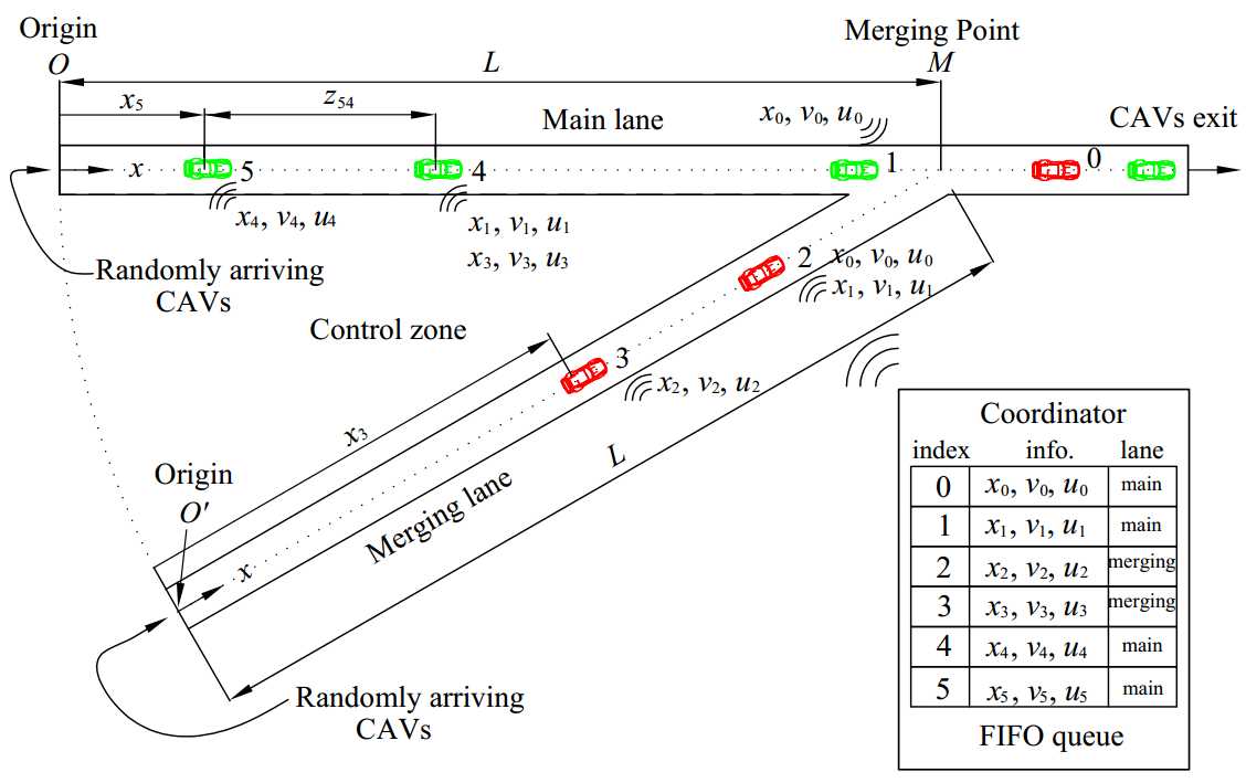
Figure 1: The merging problem

We review next the optimal merging control problem as presented in Xiao and Cassandras (2019b) so as to apply the OCBF framework to it. The vehicle dynamics for each CAV $i\in S(t)$ along the lane to which it belongs take the form

$$\left[\begin{array}[c]{c}\dot{x}_{i}(t)\\ \dot{v}_{i}(t)\end{array}\right]=\left[\begin{array}[c]{c}v_{i}(t)\\ u_{i}(t)\end{array}\right]$$ (45)

where $x_{i}(t)$ denotes the distance to the origin $O$ ($O^{\prime}$) along the main (merging) lane if the vehicle $i$ is located in the main (merging) lane, $v_{i}(t)$ denotes the velocity, and $u_{i}(t)$ denotes the control input (acceleration). We consider two objectives for each CAV subject to three constraints, as detailed next.

Objective 1 (Minimizing travel time): Let $t_{i}^{0}$ and $t_{i}^{M}$ denote the time that CAV $i\in S(t)$ arrives at the origin $O$ or $O^{\prime}$ and the MP $M$, respectively. We wish to minimize the travel time $t_{i}^{M}-t_{i}^{0}$ for CAV $i$.

Objective 2 (Minimizing energy consumption): We also wish to minimize energy consumption for each CAV $i\in S(t)$ expressed as

$$J_{i}(u_{i}(t))=\int_{t_{i}^{0}}^{t_{i}^{M}}C(u_{i}(t))dt,$$ (46)

where $C(\cdot)$ is a strictly increasing function of its argument.

Constraint 1 (Safety constraints): Let $i_{p}$ denote the index of the CAV which physically immediately precedes $i$ in the CZ (if one is present). We require that the distance $z_{i,i_{p}}(t):=x_{i_{p}}(t)-x_{i}(t)$ be constrained by the speed $v_{i}(t)$ of CAV $i\in S(t)$ so that

$$z_{i,i_{p}}(t)\geq\varphi v_{i}(t)+\delta_{0},\text{ \ }\forall t\in[t_{i}^{0},t_{i}^{M}],$$ (47)

where $\varphi$ denotes the reaction time (as a rule, $\varphi=1.8$ is used, e.g., Vogel (2003)). If we define $z_{i,i_{p}}$ to be the distance from the center of CAV $i$ to the center of CAV $i_{p}$, then $\delta_{0}$ is a constant determined by the length of these two CAVs (generally dependent on $i$ and $i_{p}$ but taken to be a constant over all CAVs for simplicity).

Constraint 2 (Safe merging): There should be enough safe space at the MP $M$ for a merging CAV to cut in, i.e.,

$$z_{1,0}(t_{1}^{M})\geq\varphi v_{1}(t_{1}^{M})+\delta_{0}.$$ (48)

Constraint 3 (Vehicle limitations): Finally, there are constraints on the speed and acceleration for each $i\in S(t)$, i.e.,

$$v_{\min}\leq v_{i}(t)\leq v_{\max},\forall t\in[t_{i}^{0},t_{i}^{M}],$$ (49)

$$u_{\min}\leq u_{i}(t)\leq u_{\max},\forall t\in[t_{i}^{0},t_{i}^{M}],$$

where $v_{\max}>0$ and $v_{\min}\geq 0$ denote the maximum and minimum speed allowed in the CZ, while $u_{\min}<0$ and $u_{\max}>0$ denote the minimum and maximum control input, respectively.

The common way to minimize energy consumption is by minimizing the control input effort $u_{i}^{2}(t)$. By normalizing travel time and $u_{i}^{2}(t)$, and using $\alpha\in[0,1]$, we construct a convex combination as in (12):

$$\begin{aligned} J_{i}(u_{i}(t))=\int_{t_{i}^{0}}^{t_{i}^{M}}\left(\alpha+\frac{(1-\alpha)\frac{1}{2}u_{i}^{2}(t)}{\frac{1}{2}\max\{u_{\max}^{2},u_{\min}^{2}\}}\right)dt\end{aligned}.$$ (50)

If $\alpha=1$, then we solve (50) as a minimum time problem. Otherwise, by defining $\beta:=\frac{\alpha\max\{u_{\max}^{2},u_{\min}^{2}\}}{2(1-\alpha)}$ and multiplying the last equation by $\frac{\beta}{\alpha}$, we have:

$$J_{i}(u_{i}(t)):=\beta(t_{i}^{M}-t_{i}^{0})+\int_{t_{i}^{0}}^{t_{i}^{M}}\frac{1}{2}u_{i}^{2}(t)dt,$$ (51)

where $\beta\geq 0$ is a weight factor that can be adjusted to penalize travel time relative to the energy cost. Note that all the constraints in the merging problem are with relative degree one.

Similar to (13), we will also include the possibility of system model uncertainties, errors due to signal transmission, as well as computation errors by adding two noise terms in (45) to get

$$\left[\begin{array}[c]{c}\dot{x}_{i}(t)\\ \dot{v}_{i}(t)\end{array}\right]=\left[\begin{array}[c]{c}v_{i}(t)+w_{i,1}(t)\\ u_{i}(t)+w_{i,2}(t)\end{array}\right]$$ (52)

where $w_{i,1}(t),w_{i,2}(t)$ denote two random processes defined in an appropriate probability space.

6 MERGING PROBLEM ANALYSIS

In this section, we first review the decentralized optimal control (OC) solution derived in Xiao and Cassandras (2019b) for those CAVs whose constraints in (47)-(49) will not become active in the CZ. This is to ensure that these solutions are indeed computationally efficient. When one or more constraints becomes active, we use the CBF method to account for these constraints and take the unconstrained optimal solution as reference. When more complex objective functions, nonlinear dynamics, and comfort are involved, we adapt the CBF method to such problems. In addition, we show how we can deal with the constraint violation problem due to perturbations, such as the noise in (52) and other unknown random events.

We need to distinguish between the following two cases: $(i)$ $i_{p}=i-1$, i.e., $i_{p}$ is the CAV immediately preceding $i$ in the FIFO queue (such as CAV 3 or 5 in Fig. 1), and $(ii)$ $i_{p}<i-1$ (such as CAV 2 or 4 in Fig. 1), which implies CAV $i-1$ is in a different lane from $i$. We can solve the merging problem for all $i\in S(t)$ in a decentralized way, in the sense that CAV $i$ can solve it using only its own local information (position, velocity and acceleration) along with that of its “neighbor” CAVs $i-1$ and $i_{p}$. Observe that if $i_{p}=i-1$, then (48) is a redundant constraint. Otherwise, we need to consider (47) and (48) independently.

Let $\bm{x}_{i}(t):=(x_{i}(t),v_{i}(t))$ be the state vector and $\bm{\lambda}_{i}(t):=(\lambda_{i}^{x}(t),\lambda_{i}^{v}(t))$ be the costate vector (for simplicity, in the sequel we omit explicit time dependence when no ambiguity arises). The Hamiltonian for the merging problem with the state, control, and safety constraints adjoined is

$$H_{i}(\bm{x}_{i},\bm{\lambda}_{i},u_{i})= \beta+\frac{1}{2}u_{i}^{2}\!+\!\lambda_{i}^{x}v_{i}+\lambda_{i}^{v}u_{i}+\mu_{i}^{a}(u_{i}\!-\!u_{max})$$ (53)

$$+\mu_{i}^{b}(u_{min}-u_{i})+\mu_{i}^{c}(v_{i}-v_{max})$$

$$+\mu_{i}^{d}(v_{min}-v_{i})+\mu_{i}^{e}(x_{i}+\varphi v_{i}+\delta_{0}-x_{i_{p}})$$

The Lagrange multipliers $\mu_{i}^{a},\mu_{i}^{b},\mu_{i}^{c},\mu_{i}^{d},\mu_{i}^{e}$ are positive when the constraints are active and become 0 when the constraints are strict. Note that when the safety constraint (47) becomes active, the expression above involves $x_{i_{p}}(t)$ in the last term. When $i=1$, the optimal trajectory is obtained without this term, since (47) is inactive over all $[t_{1}^{0},t_{1}^{M}]$. Thus, once the solution for $i=1$ is obtained, $x_{1}^{\ast}$ is a given function of time and available to $i=2$. Based on this information, the optimal trajectory of $i=2$ is obtained. Similarly, all subsequent optimal trajectories for $i>2$ can be recursively obtained based on $x_{i_{p}}^{\ast}(t)$.

6.1 CAVs with Unconstrained Optimal Control

Assuming that (47) and (49) remain inactive over $[t_{i}^{0},t_{i}^{M}]$, and the safe merging constraint (48) is not violated at $t_{i}^{M}$, we can obtain the unconstrained optimal solution as shown in Xiao and Cassandras (2019b):

$$u_{i}^{\ast}(t)=a_{i}t+b_{i}$$ (54)

$$v_{i}^{\ast}(t)=\frac{1}{2}a_{i}t^{2}+b_{i}t+c_{i}$$ (55)

$$x_{i}^{\ast}(t)=\frac{1}{6}a_{i}t^{3}+\frac{1}{2}b_{i}t^{2}+c_{i}t+d_{i}$$ (56)

where $a_{i}$, $b_{i}$, $c_{i}$ and $d_{i}$ are integration constants obtained by solving the following five nonlinear algebraic equations:

$$\frac{1}{2}a_{i}\cdot(t_{i}^{0})^{2}+b_{i}t_{i}^{0}+c_{i}=v_{i}^{0},$$ (57)

$$\frac{1}{6}a_{i}\cdot(t_{i}^{0})^{3}+\frac{1}{2}b_{i}\cdot(t_{i}^{0})^{2}+c_{i}t_{i}^{0}+d_{i}=0,$$

$$\frac{1}{6}a_{i}\cdot(t_{i}^{M})^{3}+\frac{1}{2}b_{i}\cdot(t_{i}^{M})^{2}+c_{i}t_{i}^{M}+d_{i}=L,$$

$$a_{i}t_{i}^{M}+b_{i}=0,$$

$$\beta+\frac{1}{2}a_{i}^{2}\cdot(t_{i}^{M})^{2}+a_{i}b_{i}t_{i}^{M}+a_{i}c_{i}=0.$$

Since we aim for the solution to the optimal merging problem to be obtained on-board each CAV, it is essential that the computational cost of solving these five algebraic equations for the integration constants in (54)-(56) be minimal. If MATLAB is used, it takes less than 1 second to solve these equations (Intel(R) Core(TM) i7-8700 CPU @ 3.2GHz 3.2GHz). On the other hand, when the constraints (47), (48), (49) become active, a complete OC solution can still be obtained Xiao and Cassandras (2019b), Malikopoulos et al. (2018), but the computation time varies between 3 and 30 seconds depending on whether $i_{p}$ is also safety-constrained or not. This motivates the derivation of conditions such that these constraints do not become active in the CZ.

The following assumption requires that if two CAVs arrive too close to each other, then the first one maintains its optimal terminal speed past the MP until the second one crosses it as well. This is to ensure that the first vehicle does not suddenly decelerate and cause the safety constraint to be violated during the last segment of its optimal trajectory.

Assumption 1

For a given constant $\zeta=\frac{v_{i}^{*}(t_{i}^{M})}{v_{i-1}^{*}(t_{i-1}^{M})}\varphi+\frac{\delta_{0}}{v_{i-1}^{*}(t_{i-1}^{M})}$, any CAV $i-1\in S(t)$ such that $t_{i}^{M}-t_{i-1}^{M}<\zeta$ maintains a constant speed $v_{i-1}(t)=v_{i-1}^{\ast}(t_{i-1}^{M})$ for all $t\in[t_{i-1}^{M},t_{i}^{M}]$.

Based on this mild assumption, the following theorems from Xiao and Cassandras (2019a) ensure that the constraints (47), (48), (49) are satisfied. The first identfies simple to check conditions such that the safety constraint (47) will not become active within the CZ and the second identifies conditions such that the safe merging constraint (48) will not be violated at $t_{i}^{M}$.

Theorem 3

Xiao and Cassandras (2019a) Under Assumption 1, if $\exists\varepsilon\in(0,1]$ such that $\varepsilon v_{i}^{0}\leq v_{i_{p}}^{0}$ and $t_{i}^{0}-t_{i_{p}}^{0}\geq\frac{\varphi}{\varepsilon}+\frac{\delta_{0}}{\varepsilon v_{i}^{0}}+\frac{3L(1-\varepsilon)}{v_{i_{p}}^{0}+2v_{i_{p}}^{*}(t_{i_{p}}^{M})}$, then, under optimal control (54) for both $i$ and $i_{p}$, $z_{i,i_{p}}(t_{i}^{M})\geq\varphi v_{i}(t_{i}^{M})+\delta_{0}$. Moreover, if $\exists t_{p}\in[t_{i}^{0},t_{i_{p}}^{M})$ solved by $v_{i}(t_{p})+\varphi u_{i}(t_{p})-v_{i_{p}}^{*}(t_{p})=0$ such that the safety constraint (47) is satisfied at $t_{p}$, then $z_{i,i_{p}}(t)>\varphi v_{i}(t)+\delta_{0},\forall t\in[t_{i}^{0},t_{i}^{M}]$.

Theorem 4

Xiao and Cassandras (2019a) Let $i-1>i_{p}$. Under Assumption 1, if $\exists\varepsilon\in(0,1]$ such that $\varepsilon v_{i}^{0}\leq v_{i-1}^{0}$ and $t_{i}^{0}-t_{i-1}^{0}\geq\frac{\varphi}{\varepsilon}+\frac{\delta_{0}}{\varepsilon v_{i}^{0}}+\frac{3L(1-\varepsilon)}{v_{i-1}^{0}+2v_{i-1}^{*}(t_{i-1}^{M})}$, then, under optimal control (54) for both $i$ and $i-1$, the safe merging constraint (48) is satisfied.

Finally, the next result provides conditions such that the speed constraint in (49) will be satisfied within the CZ:

Theorem 5

Xiao and Cassandras (2019a) If $v_{i}^{0}\leq v_{0},\forall i\in S(t)$ for $v_{0}\in[v_{\min},v_{\max})$, $\beta>0$ and under optimal control (54), then for any $L\leq L_{\max}$, the speed limitations in (49) are satisfied $\forall t\in[t_{i}^{0},t_{i}^{M}],\forall i\in S(t)$. Where

$$L_{\max}=\sqrt{\frac{8v_{\max}^{4}-6v_{\max}^{2}v_{0}^{2}-2v_{\max}v_{0}^{3}}{9\beta}}$$

Note that all conditions in Theorems 3-5 are based on the initial conditions $v_{i}^{0},t_{i}^{0}$ of CAV $i\in S(t)$ and information from other CAVs ahead of $i$. Although the conditions in Theorem. 5 pertain to all CAVs, it can also be easily applied to each individual CAV $i\in S(t)$. The case of control constraints being active is addressed in the following remark.

Remark 2

If the conditions in Theorems 3-5 are satisfied for CAV $i\in S(t)$, but the control constraint in (49) is initially violated at $u_{max}$ (since we have that $a_{i}<0$ $(\beta\neq 0)$ and $u_{i}(t_{i}^{M})=0$ when $i$ is under unconstrained OC (54) Xiao and Cassandras (2019b)), then the safety constraint (47), the safe merging constraint (48) and the speed constraint in (49) are all satisifed when we first apply $u_{max}$ starting at $t_{i}^{0}$ followed by an unconstrained OC. This is obvious since the $u_{max}$-constrained OC has lower speed compared with the unconstrained OC (54). The derivation of the unconstrained OC after the $u_{max}$-constrained arc is easy and time efficient (similar to (54)).

Once we confirm that a CAV $i\in S(t)$ meets all conditions in Theorems 3-5 (the control constraint violation case is discussed in Remark 2 and also viewed as an unconstrained OC), we can directly apply the unconstrained control (54) to CAV $i$. Considering the noisy dynamics (52), we wish to find a controller that tracks both the optimal speed (55) and position (56) since the safety constraint (47) and the safe merging constraint (48) both depend on the speed and position. We use the position and speed exponential feedback control forms in (23)-(25).

Extensive simulation results (see Xiao and Cassandras (2019a)) have shown that the ratio of CAVs that satisfy the conditions in Theorems 3-5 is large under normal (not exceedingly high) traffic conditions. Still, when these conditions are not satisfied for some CAV $i\in S(t)$, we can use the OCBF method to account for these constraints as shown in the sequel.

6.2 OCBF for the Merging Problem

Suppose that an unconstrained OC solution is available for the objective (51), obtained through (54)-(56). Our goal here is to determine a controller for those CAVs that do not satisfy the conditions in Theorems 3-5. This is achieved by combining the unconstrained OC solution with a CBF-based controller leading to an OCBF controller whose goal is to track the former as closely as possible.

First, we aim to track the optimal speed $v_{i}^{\ast}(t)$ obtained through (54)-(56). In particular, we define a controller aiming to drive $v_{i}(t)$ to $v_{ref}(t)$ using the form (28) or (27). Using either form of $v_{ref}(t)$, we can now proceed as in (29) and define an output $y_{i}(t):=v_{i}(t)-v_{ref}(t)$ and a CLF $V(y_{i}(t))=y_{i}^{2}(t)$. The control should satisfy the CLF constraint (29).

Second, we deal with the safety and vehicle limitation constraints (Constraints 1,3) using HOCBFs to map them from the state $\bm{x}_{i}(t)$ to the control input $u_{i}(t)$. In particular, define CBFs $b_{i,q}(\bm{x}_{i}(t)),$ $q\in\{1,2,3\}$ where $b_{i,1}(\bm{x}_{i}(t))=v_{max}-v_{i}(t),$ $b_{i,2}(\bm{x}_{i}(t))=v_{i}(t)-v_{min},$ $b_{i,3}(\bm{x}_{i}(t))=z_{i,i_{p}}(t)-\varphi v_{i}(t)-\delta_{0}$. The relative degree of each $b_{i,q},$ $q\in\{1,2,3\}$ is 1. Therefore, in Definition 4, we choose a HOCBF with $m=1$. Any control should satisfy the HOCBF constraints (30) and (31). Note that $u_{i}(t)\in[u_{\min},u_{\max}]$ is already a constraint on the control input, hence, we do not need to use a HOCBF for it.

Finally, the safe merging constraint (48) ensures that there are no collisions when CAVs from different lanes arrive at the merging point $M$. It is only imposed at $t_{1}^{M}$ and does not apply to all $t\in[t_{i}^{0},t_{i}^{M})$. For example, vehicles 4 and 3 in Fig. 1 are not constrained before they arrive at the merging point $M$, but have to satisfy (48) at $M$. In order to use a HOCBF approach, we need a version of (48) that is continuous in time when $i-1>i_{p}$. Vehicles $i$ and $i-1$ both arrive randomly at $O$ or $O^{\prime}$, and the minimum distance along the lane $z_{i,i-1}(t_{i}^{0})$ between vehicle $i$ and $i-1$ is 0, i.e., these two CAVs are allowed to arrive at the origin $O$ or $O^{\prime}$ at the same time. The coordinator FIFO queue preserves the arrival order of $i$ and $i-1$ at $O$ or $O^{\prime}$ at the merging point $M$. When vehicles $i$ and $i-1$ arrive at $M$, they will merge into the same lane. Therefore, the distance between $i$ and $i-1$ must be greater than or equal to $\varphi v_{i}(t_{i}^{M})+\delta_{0}$, which is in the form of (48). However, we have considerable freedom in choosing the reaction time $\varphi$ from (48) for vehicle $i$ ($i-1>i_{p}$)  for all $t\in(t_{i}^{0},t_{i}^{M})$. In the following, we provide a definition for the allowed variation of $\varphi$:

Definition 7

The reaction time $\varphi$ for vehicle $i$ ($i-1>i_{p}$) is a strictly increasing function $\Phi:\mathbb{R}\rightarrow\mathbb{R}$ that satisfies the initial condition $\Phi(x_{i}(t_{i}^{0}))=-\frac{\delta_{0}}{v_{i}^{0}}$ and final condition $\Phi(x_{i}(t_{i}^{M}))=\varphi$.

As an example, in Fig. 1 where $x_{i}(t_{i}^{0})=0$ and $x_{i}(t_{i}^{M})=L$, we have $\Phi(x_{i}(t))=\frac{\varphi x_{i}(t)}{L}$ if $\delta_{0}=0$. The lower bound of the distance from (48) becomes greater as vehicle $i$ approaches the merging point $M$ such that there is adequate space for the vehicle in the merging lane to join the main lane. Therefore, a continuous version of the constraint from (48) on $i$ for $i-1>i_{p}$ in the control zone is:

$$z_{i,i-1}(t)\geq\Phi(x_{i}(t))v_{i}(t)+\delta_{0},\text{ \ \ }\forall t\in[t_{i}^{0},t_{i}^{M}].$$ (58)

The relative degree of (58) is 1. To enforce safe merging, we employ a HOCBF that is similar to the ones used for safety (30).

6.2.1 OCBF controller

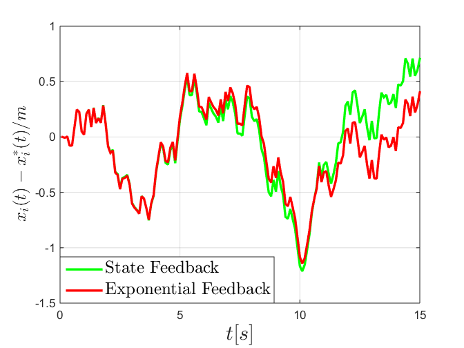
(a) Tracking position error comparison.

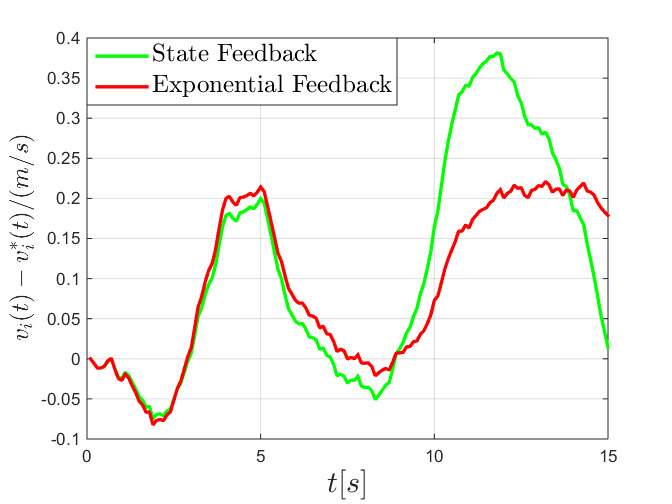
(b) Tracking speed error comparison.

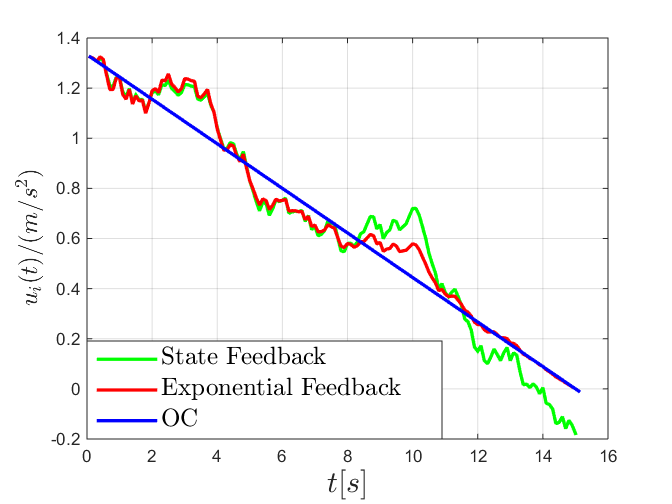
(c) Control profile comparison.

Figure 2: Tracking performance comparison with vehicle noise between the state feedback control (25) and the exponential feedback control (23) with vehicle limitations (49).

Along the lines of Sec. 4.2, we now seek a control input $u_{i}(t)$ in the HOCBF method which tracks the unconstrained optimal control $u_{i}^{\ast}(t)$ through a HOCBF controller aiming to drive $u_{i}(t)$ to $u_{ref}(t)$ defined by (24) or (23).

Following the OCBF approach in Sec. 4.2, we apply (32) and consider the objective function:

$$J_{i}(u_{i}(t),\delta_{i}(t))\!=\!\int_{t_{i}^{0}}^{t_{i}^{M}}\!\left(\beta\delta_{i}^{2}(t)\!+\!\frac{1}{2}(u_{i}(t)\!-\!u_{ref}(t))^{2}\right)dt,$$ (59)

subject to (52), the corresponding HOCBF constraints as (30), (31), and the CLF constraint (29), the initial and terminal conditions $x_{i}(t_{i}^{0})=0$, $x_{i}(t_{i}^{M})=L$, and given $t_{i}^{0},v_{i}(t_{i}^{0})$. Thus, we have combined the HOCBF method and the OC solution by using (24) or (23) to link the optimal position and acceleration to $u_{ref}(t)$, and use (28) or (27) in the CLF $(v_{i}(t)-v_{ref}(t))^{2}$ to combine with (59). The resulting optimal $u_{i}(t)$ in (59) is the OCBF control.

As in (33), we partition the continuous time interval $[t_{i}^{0},t_{i}^{M}]$ into equal time intervals $\{[t_{i}^{0}+k\Delta t,t_{i}^{0}+(k+1)\Delta t)\},$ $k=0,1,2,\dots$ In each interval $[t_{i}^{0}+k\Delta t,t_{i}^{0}+(k+1)\Delta t)$, we assume the control is constant and find a solution to the optimization problem (59). Specifically, at $t=t_{i}^{0}+k\Delta t$ ($k=0,1,2,\dots$), we solve

$$\underset{t=t_{i}^{0}+k\Delta t}{\mathbf{QP:}}\bm{u}_{i}^{\star}(t)=\mathop{\arg\min}_{\bm{u}_{i}(t)}\frac{1}{2}\bm{u}_{i}(t)^{T}H\bm{u}_{i}(t)+F^{T}\bm{u}_{i}(t)$$ (60)

$${\small\bm{u}_{i}(t)=\left[\begin{array}[c]{c}u_{i}(t)\\ \delta_{i}(t)\end{array}\right],}\text{ \ }{\small H=\left[\begin{array}[c]{cc}1&0\\ 0&\beta\end{array}\right],}\text{ \ }{\small F=\left[\begin{array}[c]{c}-u_{ref}(t)\\ 0\end{array}\right]}$$

subject to the constraints as (34)-(36) as they pertain to the merging problem. After solving (60) and get an optimal control ${u}_{i}^{\star}(t)$, we update (52) for all $t\in(t_{i}^{0}+k\Delta t,t_{i}^{0}+(k+1)\Delta t)$. As shown in Sec. 7, the use of only (28) or (27), yields an OCBF control which is Lipschitz continuous, whereas using both state and control trackings improves performance.

7 SIMULATION RESULTS

All controllers in this section have been implemented using MATLAB and we have used the Vissim microscopic multi-model traffic flow simulation tool as a baseline for the purpose of making comparisons between our controllers and human-driven vehicles adopting standard car-following models used in Vissim. We used quadprog for solving QPs of the form (59) or (66) and ode45 to integrate the vehicle dynamics.

Referring to Fig. 1, CAVs arrive according to Poisson processes with arrival rates that we allow to vary in our simulation examples. The initial speed $v_{i}(t_{i}^{0})$ is also randomly generated with uniform distribution in $[15m/s,20m/s]$ at the origins $O$ and $O^{\prime}$, respectively. The parameters for (59) or (66) and (52) are: $L=400m,\varphi=1.8s,$ $\delta_{0}=0m,u_{max}=3.924m/s^{2},$ $u_{min}=-3.924m/s^{2},$ $v_{max}=30m/s,v_{min}=0m/s,$ $\beta=1,$ $\epsilon=10,$ $\Delta t=0.1s,$ $c=1$, and we consider uniformly distributed noise processes (in [-2, 2] for $w_{i,1}(t)$ and in [-0.2, 0.2] for $w_{i,2}(t)$) for all simulations. The value of $\Delta t$ is chosen as small as possible, depending on computational resources available, in order to address the inter-sampling effect on the HOCBFs and maintain a guaranteed satisfaction of all constraints.

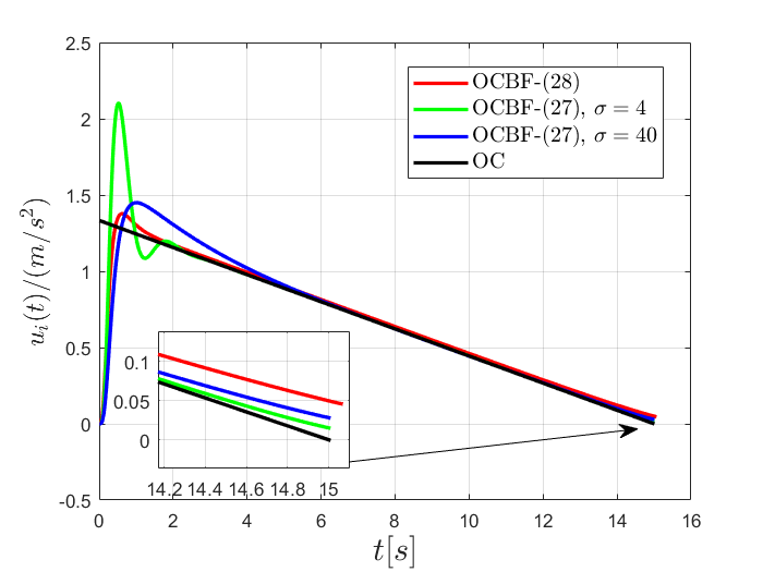
(a) Controls with only speed tracking (28) or (27).

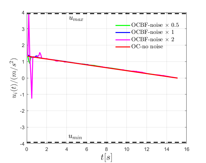
(b) Controls with both (28) and (24) under different noise levels.

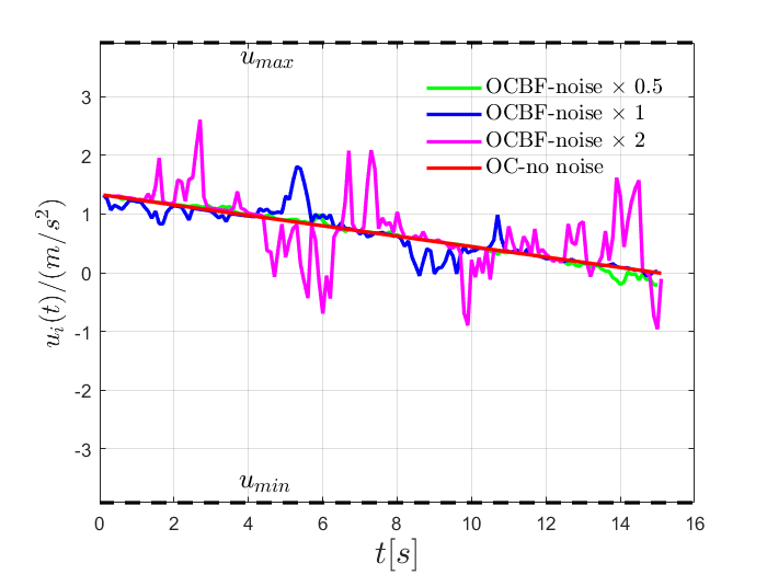
(c) Controls with (27) and (23), $\sigma\!=\!40$ under different noise levels.

Figure 3: OCBF implementation examples under different tracking equations and noise levels with vehicle limitations (49).

1. Position and speed feedback tracking implementation example. First, we provide a simple example of the tracking control implementation for a single vehicle which considers (59) as the objective function and employs the unconstrained optimal control (54). Although we do not consider the vehicle noise, there is still discretization ($\Delta t=0.1s$) error in the implementation. The initial parameters are $t_{i}^{0}=0s$, $v_{i}^{0}=20m/s$, $\alpha=0.26$. We first consider the comparison between exponential feedback control (23) and directly applied unconstrained control (54), as shown in terms of average tracking errors in Table 1. We can see that the feedback control (23) can significantly improve both average tracking errors. The tracking errors decrease as $\sigma_{1},\sigma_{2}$ decrease, consistent with the argument after (23) that we wish to make $\sigma_{1}<\sigma_{2}$, as shown from the 3rd and 5th columns in Table 1.

Table 1: Average tracking error comparison without vehicle noise

Items	$u^{*}(t)$ (54)	Feedback control (23)
$\sigma_{1},\sigma_{2}$		4, 12	6, 16	12, 4
$\frac{1}{2}u_{i}^{2}(t)$	4.4000	4.4396	4.4366	4.4318
Pos. err.	-0.1678	-0.0280	-0.0452	-0.0577
Spd. err.	-0.0333	-0.0037	-0.0059	-0.0095

Then, under the same randomly generated noise $w_{i,1}(t)\in[2m/s,-2m/s]$ and $w_{i,2}(t)\in[-0.1m/s^{2},0.1m/s^{2}]$, we compare the tracking performance between the state feedback control (25) ($k_{1}=0.25,k_{2}=0.1$) and the exponential feedback control (23) ($\sigma_{1}=4,\sigma_{2}=10$, the same coefficients as in (25)), as shown in Fig. 2(a)-2(c). We can see that the exponential feedback control (23) can perform almost the same when the control $u_{i}^{\ast}(t)$ is large and outperforms the state feedback control (25) as the optimal control become smaller. The control input in the exponential feedback control input (23) varies less than the state feedback control (25), as shown in Fig. 2(c).

2. OCBF implementation example. Next, we provide a simple example of the OCBF controller implementation for a single vehicle which considers (59) as the objective function. The initial parameters are the same as the last example. If we only apply (28) or (27), set $u_{ref}(t)=0$ and assume no noise, then we obtain the control profiles shown in Fig. 3(a). The speed reference form (27) tends to achieve a closer track of the OC control (black curve) compared to the form (28) at the expense of larger over-shot; as a result, performnace is worse as shown in Table 2 (values in red are the best).

If we apply both (28) and (24) without noise, we obtain the control profiles shown in where the OCBF controller’s performance is virtually indistinguishable from that of the OC control, as shown in Table 2.

With noise added (based on a uniform distribution in [-2, 2] for $w_{i,1}(t)$ and in [-0.2, 0.2] for $w_{i,2}(t)$), we show the control profiles under different noise levels in Fig. 3(b) with (28) and (24); and in Fig. 3(c) with (27) and (23). Constraints 1-3 may be temporarily violated but will be forced to be satisfied again in finite time through constraint (41). The speed and control tracking forms (28) and (24) perform better than (27) and (23) as noise increases.

Table 2: Objective function comparison without noise

Items	OC	OCBF
Track		(28)	(27)	(27)	(28), (24)
$\sigma$			4	40
time (s)	15.01	15.07	15.01	15.01	15.01
$\frac{1}{2}u_{i}^{2}(t)$	4.44	4.41	4.6962	4.66	4.44
objective	33.33	33.43	33.52	33.50	33.34

3. Comparison of OC control from Xiao and Cassandras (2019b), CBF control from Xiao et al. (2019a), and OCBF control in this paper. Consider the merging problem with the simple objective function (51) for which we can easily get unconstrained optimal solutions. Then, we employ the CBF method and the OCBF technique (with (28) and (24)) introduced in Sec. 6.2. Simulation results under four different trade-off parameters are shown in Table 3. We can see that the OCBF method achieves comparable results to OC, even in the presence of noise.

The computation time in MATLAB with the OCBF method for each $i$ at each step is less than 0.01s (Intel(R) Core(TM) i7-8700 CPU @ 3.2GHz$\times 2$), while the OC method takes between $1s$ and $30s$ for each CAV, depending on whether the constraints are active or not.

Table 3: Comparison (data in average) of OC, CBF and OCBF (with noise)

Method	$\alpha$	Noi.	Time($s$)	$\frac{1}{2}u_{i}^{2}(t)$	Obj.
CBF	N/A	no	14.6978	26.9178	N/A
OC	$0.01$	no	$\bm{25.4291}$	$\bm{0.1725}$	$\bm{2.1288}$
OCBF		no	25.6879	1.0582	3.0256
		yes	25.7494	2.2373	4.1976
OC	$0.25$	no	$\bm{17.0472}$	$\bm{4.9069}$	$\bm{36.4909}$
OCBF		no	17.1176	5.5569	37.1139
		yes	17.1396	6.8959	38.1605
OC	$0.40$	no	$\bm{15.1713}$	$\bm{10.6508}$	$\bm{53.1120}$
OCBF		no	15.2286	11.3629	53.7157
		yes	15.2527	12.7671	54.6325
OC	$0.60$	no	$\bm{13.1035}$	$\bm{24.4079}$	$\bm{70.2922}$
OCBF		no	13.1560	25.2468	70.8720
		yes	13.1692	26.6534	71.4938

We also show in Fig. 4 how the travel time and energy consumption vary as the weight factor $\alpha$ in (50) changes. The significance of Fig. 4 is to show how well the OCBF can match the optimal performance obtained through OC. Examples of the barrier function profiles for the safety constraint (47) under known and unknown noise bound $\bm{W}$ are shown in Fig. 5. If $\bm{W}$ is known, the safety constraint (47) is guaranteed with some conservativeness; Otherwise, the safety constraint (47) is satisfied most of the time without conservativeness.

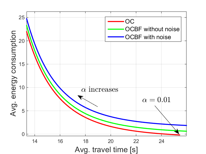
Figure 4: Travel time and energy consumption as the factor $\alpha$ changes.

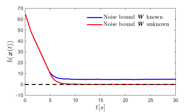
Figure 5: Barrier function $b(\bm{x})$ under noise $w_{i,1}(t)\in[-4,4]m/s,w_{i,2}(t)\in[-0.4,0.4]m/s^{2}$. $b(\bm{x})\geq 0$ denotes the satisfaction of the safety constraint (47).

4. Comparison of CBF control from Xiao et al. (2019a), CBF control with objective (61) in this paper, and human-driven vehicles through Vissim. This simulation refers to A for the case that the objective function is too complex to get explicit optimal solutions. We consider the objective function (61) which is too complex to allow the derivation of an OC solution. Thus, we solve (61) through the sequence of QPs (66) and select a value $\beta=0.2$ in (66) through trial and error to best match the performance in Vissim. We vary the relative traffic arrival rates of the main and merging lane and show our results in Tables 4, 5, 6.

In Tables 4 and 5, note that both CBF methods outperform human-driven vehicles modeled though Vissim. We also observe that the CBF method developed in this paper using (61) is vastly superior to that of Xiao et al. (2019a) in the energy component with little loss in travel time performance. We also note that without any control (as in Vissim), the main lane vehicles have priority over the merging lane and the merging lane vehicles may even stop before the merging point. Thus, there is heavy congestion in the merging lane when the ratio between the main lane and merging lane arrival rates is 1:3.

We observe in Table 6 that the energy consumption of vehicles in Vissim is significantly lower compared to the CBF methods. This is due to the fact that the merging lane vehicles frequently stop before the merging point $M$, thus having low speeds when passing over $M$. In order to achieve a fair comparison, we consider a longer time horizon over which we measure fuel consumption and travel time. This is accomplished by extending the trip of each vehicle for an additional length $L$ beyond the merging point $M$, as shown in Table 7. As expected, the overall energy performance under CBF control is now significantly better (by about 37%) than that of human-driven vehicles.

Table 4: Main lane arrival rate : Merging lane arrival rate = 1:1

Items	CBF-(51)	CBF-(61)	Vissim
Ave. time($s$)	$\bm{14.6978}$	18.1549	25.0813
Main time($s$)	$\bm{14.7000}$	18.1717	17.9935
Merg. time($s$)	$\bm{14.6956}$	18.1378	32.3267
Ave. fuel($mL$)	57.9532	$\bm{30.9813}$	36.9954
Main fuel($mL$)	57.7028	$\bm{30.8856}$	42.6925
Merg. fuel($mL$)	58.2092	$\bm{31.0791}$	31.1717

Table 5: Main lane arrival rate : Merging lane arrival rate = 3:1

Items	CBF-(51)	CBF-(61)	Vissim
Ave. time($s$)	$\bm{14.6578}$	18.1189	23.9300
Main time($s$)	$\bm{14.6794}$	18.1413	18.3476
Merg. time($s$)	$\bm{14.6074}$	18.0667	36.9556
Ave. fuel($mL$)	60.2624	$\bm{31.9754}$	39.8587
Main fuel($mL$)	61.0934	$\bm{32.7556}$	42.8554
Merg. fuel($mL$)	58.3235	$\bm{30.1549}$	32.8666

Table 6: Main lane arrival rate : Merging lane arrival rate = 1:3

Items	CBF-(51)	CBF-(61)	Vissim
Ave. time($s$)	$\bm{14.6000}$	18.0093	29.2035
Main time($s$)	$\bm{14.7133}$	18.1133	17.8667
Merg. time($s$)	$\bm{14.5761}$	17.9873	31.5986
Ave. fuel($mL$)	61.1607	33.4848	$\bm{30.5212}$
Main fuel($mL$)	57.3805	$\bm{30.9263}$	46.5004
Merg. fuel($mL$)	61.9593	34.0253	$\bm{27.1454}$

Table 7: Rate = 1:3, adding a lane of length $L$ after the merging point.

Items	CBF-(51)	CBF-(61)	Vissim
Ave. time($s$)	$\bm{28.7975}$	36.3076	50.9987
Main time($s$)	$\bm{28.9857}$	36.3786	38.8643
Merg. time($s$)	$\bm{28.7569}$	36.2923	53.6123
Ave. fuel($mL$)	88.2784	$\bm{51.6414}$	81.6633
Main fuel($mL$)	86.6246	$\bm{48.7578}$	77.8110
Merg. fuel($mL$)	88.6347	$\bm{52.2625}$	82.4930

8 CONCLUSIONS

We have developed a real-time framework that combines optimal trajectories generated through optimal control with the computationally efficient HOCBF method providing safety guarantees. This allows us to deal with cases where the optimal control solution becomes computationally costly, as well as to handle the presence of noise in the system dynamics by exploiting the ability of HOCBFs to add some robustness to an optimal controller. We applied the proposed framework to the traffic merging problem for connected and automated vehicles with results showing significant improvement in performance compared with human driven vehicles. An ongoing research challenge is imparting adaptivity to HOCBF-based controllers with respect to a changing environment. Regarding autonomous vehicles (CAVs) in a traffic network, ongoing work is aimed at integrating them with non-CAVs.

Appendix A Complex Objectives, Dynamics and Comfort

As shown in Xiao et al. (2019a), the HOCBF method allows us to deal with nonlinear systems and to consider more complex objective functions than (51). In particular, we consider:

$$\min_{u_{i}(t)}\beta(t_{i}^{M}-t_{i}^{0})+\int_{t_{i}^{0}}^{t_{i}^{M}}f_{v}(t)dt,$$ (61)

where $f_{v}(t)$ represents a more detailed realistic energy model replacing the simple expression $u_{i}^{2}(t)$ commonly used as a surrogate energy function. As an example, we have adopted in Xiao et al. (2019a) the following energy model from Kamal et al. (2013), which describes fuel consumed per second as

$$f_{v}(t) =f_{cruise}(t)+f_{accel}(t),$$ (62)

$$f_{cruise}(t) =\omega_{0}+\omega_{1}v_{i}(t)+\omega_{2}v_{i}^{2}(t)+\omega_{3}v_{i}^{3}(t),$$

$$f_{accel}(t) =(r_{0}+r_{1}v_{i}(t)+r_{2}v_{i}^{2}(t))u_{i}(t).$$

where $\omega_{0}$, $\omega_{1}$, $\omega_{2}$, $\omega_{3}$, $r_{0}$, $r_{1}$ and $r_{2}$ are positive coefficients (typical values are reported in Kamal et al. (2013)). It is assumed that during braking, i.e., $u_{i}(t)<0$, no fuel is consumed. Note that (61) is hard to solve through an OC analysis as in the previous section. However, in the HOCBF approach this can be handled numerically.

As for the dynamics of CAVs, the HOCBF method can easily handle nonlinear dynamics instead of just the linear form in (45). Thus, we use the vehicle dynamics Khalil (2002):

$$\underbrace{\left[\begin{array}[c]{c}\dot{x}_{i}(t)\\ \dot{v}_{i}(t)\end{array}\right]}_{\dot{\bm{x}}_{i}(t)}=\underbrace{\left[\begin{array}[c]{c}v_{i}(t)\\ -\frac{1}{m_{i}}F_{r}(v_{i}(t))\end{array}\right]}_{f(\bm{x}_{i}(t))}+\underbrace{\left[\begin{array}[c]{c}0\\ \frac{1}{m_{i}}\end{array}\right]}_{g(\bm{x}_{i}(t))}u_{i}(t),$$ (63)

where $m_{i}$ denotes the mass of CAV $i$, and $v_{i}(t)$ is its velocity. $F_{r}(v_{i}(t))$ denotes the resistance force, which is normally expressed Khalil (2002) as:

$$F_{r}(v_{i}(t))=k_{0}sgn(v_{i}(t))+k_{1}v_{i}(t)+k_{2}v_{i}^{2}(t),$$ (64)

where $k_{0}>0,k_{1}>0$ and $k_{2}>0$ are scalars determined empirically, and $sgn$ is the signum function. The first term in $F_{r}(v_{i}(t))$ denotes the Coulomb friction force, the second term denotes the viscous friction force and the last term denotes the aerodynamic drag.

In the HOCBF method, we do not explicitly optimize the travel time shown in (61). Instead, we use a CLF to drive $v_{i}(t)$ to a desired speed such that the travel time is optimized. In Xiao et al. (2019a), we define an output $y_{i}(t):=v_{i}(t)-v_{max}$ and choose a CLF $V(y_{i}(t))=y_{i}^{2}(t)$. Any control input $u_{i}(t)$ should satisfy, for all $t\in[t_{i}^{0},t_{i}^{M}]$,

$$L_{f}V(y_{i}(t))+L_{g}V(y_{i}(t))u_{i}(t)+\epsilon V(y_{i}(t))\leq\delta_{i}(t)$$ (65)

where $\epsilon>0$ and $\delta_{i}(t)$ is a relaxation variable that makes the requirement $v_{i}(t)=v_{max}$ to be treated as a soft constraint. Thus, we seek to achieve Objective 1 indirectly and consider Objective 2 directly, replacing (61) by

$$\min_{u_{i}(t),\delta_{i}(t)}\int_{t_{i}^{0}}^{t_{i}^{M}}\left(f_{v}(t)+\beta\delta_{i}^{2}(t)\right)dt$$ (66)

subject to the same constraints as in (59) and dynamics (63). We use the QP-based method as introduced in the last subsection to solve (66). Thus, all CAVs can safely pass over the merging point $M$ while minimizing $J_{i}(u_{i}(t),\delta_{i}(t))$ within each time interval, hence jointly minimizing the energy consumption captured by $f_{v}(t)$ and travel time (indirectly) through the minimization of $\delta_{i}^{2}$. By adjusting the weight $\beta$ in (66), we can trade off between these two objectives.

When comfort is also concerned in the objective, i.e., we also want to minimize the jerk of each CAV $i$, we can directly incorporate the jerk into (66). Noting that $f_{v}(t)$ in (66) is linear in $u_{i}(t)$, we wish to formulate a Linear Program (LP) instead of a QP since the LP tends to be around 30% more computationally efficient than the QP, as shown in Xiao et al. (2019a). Including the comfort requirement, we have

$$\min_{u_{i}(t),\delta_{i}(t)}\int_{t_{i}^{0}}^{t_{i}^{M}}f_{v}(t)\!+\!\beta_{1}\delta_{i}(t)\!+\!\beta_{2}\left|\frac{u_{i}(t)\!-\!u_{i}^{\ast}(t\!-\!k\Delta t)}{\Delta t}\right|dt$$ (67)

where $u_{i}^{\ast}(t-k\Delta t)$ denotes the optimal control from the last time interval (initially set to 0 at $t_{i}^{0}$), and is known. The parameters $\beta_{1}>0,$ $\beta_{2}>0$ trade off fuel consumption, travel time, and comfort. The LP (67) is subject to the same constraints as the QP (66).

References

- Ames et al. (2012) Ames, A.D., Galloway, K., Grizzle, J.W., 2012. Control lyapunov functions and hybrid zero dynamics, in: Proc. of 51rd IEEE Conference on Decision and Control, pp. 6837–6842.
- Ames et al. (2017) Ames, A.D., Xu, X., Grizzle, J.W., Tabuada, P., 2017. Control barrier function based quadratic programs for safety critical systems. IEEE Transactions on Automatic Control 62, 3861–3876.
- Ansari and Murphey (2016) Ansari, A.R., Murphey, T.D., 2016. Sequential action control: Closed-form optimal control for nonlinear and nonsmooth systems. IEEE Transactions on Robotics 32, 1196–1214.
- Aubin (2009) Aubin, J.P., 2009. Viability theory. Springer.
- Bemporad et al. (2002) Bemporad, A., Borrelli, F., Morari, M., 2002. Model predictive control based on linear programming, the explicit solution. IEEE transactions on automatic control 47, 1974–1985.
- Boyd and Vandenberghe (2004) Boyd, S.P., Vandenberghe, L., 2004. Convex optimization. Cambridge university press, New York.
- Bryson and Ho (1969) Bryson, Ho, 1969. Applied Optimal Control. Ginn Blaisdell, Waltham, MA.
- Cao et al. (2015) Cao, W., Mukai, M., Kawabe, T., 2015. Cooperative vehicle path generation during merging using model predictive control with real-time optimization. Control Engineering Practice 34, 98–105.
- Chitour et al. (2012) Chitour, Y., Jean, F., Mason, P., 2012. Optimal control models of goal-oriented human locomotion. SIAM Journal on Control and Optimization 50, 147–170.
- Freeman and Kokotovic (1996) Freeman, R.A., Kokotovic, P.V., 1996. Robust Nonlinear Control Design. Birkhauser.
- Galloway et al. (2015) Galloway, K., Sreenath, K., Ames, A.D., Grizzle, J., 2015. Torque saturation in bipedal robotic walking through control lyapunov function based quadratic programs. IEEE Access 50, 323–332.
- Garcia and Prett (1989) Garcia, C.E., Prett, D.M., 1989. Model predictive control: theory and practice. Automatica 25, 335–348.
- Glotfelter et al. (2017) Glotfelter, P., Cortes, J., Egerstedt, M., 2017. Nonsmooth barrier functions with applications to multi-robot systems. IEEE control systems letters 1, 310–315.
- Kamal et al. (2013) Kamal, M., Mukai, M., Murata, J., Kawabe, T., 2013. Model predictive control of vehicles on urban roads for improved fuel economy. IEEE Transactions on Control Systems Technology 21, 831–841.
- Khalil (2002) Khalil, H.K., 2002. Nonlinear Systems. Prentice Hall, third edition.
- Levine and Athans (1966) Levine, W., Athans, M., 1966. On the optimal error regulation of a string of moving vehicles. IEEE Transactions on Automatic Control 11, 355–361.
- Lindemann and Dimarogonas (2019) Lindemann, L., Dimarogonas, D.V., 2019. Control barrier functions for multi-agent systems under conflicting local signal temporal logic tasks. IEEE Control Systems Letters 3, 757–762.
- Malikopoulos et al. (2018) Malikopoulos, A.A., Cassandras, C.G., Zhang, Y.J., 2018. A decentralized energy-optimal control framework for connected and automated vehicles at signal-free intersections. Automatica 2018, 244–256.
- Mayne (2014) Mayne, D., 2014. Model predictive control: Recent developments and future promise. Automatica 50, 2967–2986.
- Milanes et al. (2012) Milanes, V., Godoy, J., Villagra, J., Perez, J., 2012. Automated on-ramp merging system for congested traffic situations. IEEE Transactions on Intelligent Transportation Systems 12, 500–508.
- Mita et al. (2001) Mita, T., Nam, T.K., Hyon, S.H., 2001. Analytical time optimal control solution for a 2-link free flying acrobots, in: Proc. of IEEE International Conference on Robotics and Automation, pp. 2741–2746.
- Mukai et al. (2017) Mukai, M., Natori, H., Fujita, M., 2017. Model predictive control with a mixed integer programming for merging path generation on motor way, in: Proc. IEEE Conference on Control Technology and Applications, pp. 2214–2219, Mauna Lani.
- Nguyen and Sreenath (2016) Nguyen, Q., Sreenath, K., 2016. Exponential control barrier functions for enforcing high relative-degree safety-critical constraints, in: Proc. of the American Control Conference, pp. 322–328.
- Ntousakis et al. (2016) Ntousakis, I.A., Nikolos, I.K., Papageorgiou, M., 2016. Optimal vehicle trajectory planning in the context of cooperative merging on highways. Transportation Research Part C 71, 464–488.
- Panagou et al. (2013) Panagou, D., Stipanovic, D.M., Voulgaris, P.G., 2013. Multi-objective control for multi-agent systems using lyapunov-like barrier functions, in: Proc. of 52nd IEEE Conference on Decision and Control, Florence, Italy. pp. 1478–1483.
- Prajna et al. (2007) Prajna, S., Jadbabaie, A., Pappas, G.J., 2007. A framework for worst-case and stochastic safety verification using barrier certificates. IEEE Transactions on Automatic Control 52, 1415–1428.
- Raravi et al. (2007) Raravi, G., Shingde, V., Ramamritham, K., Bharadia, J., 2007. Merge algorithms for intelligent vehicles. In: Sampath, P., Ramesh, S. (Eds.), Next Generation Design and Verification Methodologies for Distributed Embedded Control Systems. Springer, Waltham, MA.
- Rathgeber et al. (2015) Rathgeber, C., Winkler, F., Kang, X., Muller, S., 2015. Optimal trajectories for highly automated driving. International Journal of Mechanical, Aerospace, Industrial, Mechatronic and Manufacturing Engineering 9, 946–952.
- Rios-Torres and Malikopoulos (2017) Rios-Torres, J., Malikopoulos, A., 2017. Automated and cooperative vehicle merging at highway on-ramps. IEEE Transactions on Intelligent Transportation Systems 18, 780–789.
- Scarinci and Heydecker (2014) Scarinci, R., Heydecker, B., 2014. Control concepts for facilitating motorway on-ramp merging using intelligent vehicles. Transport Reviews 34, 775–797.
- Schrank et al. (2015) Schrank, B., Eisele, B., Lomax, T., Bak, J., 2015. The 2015 urban mobility scorecard. Texas A&M Transportation Institute. URL: http://mobility.tamu.edu.
- Sontag (1983) Sontag, E., 1983. A lyapunov-like stabilization of asymptotic controllability. SIAM Journal of Control and Optimization 21, 462–471.
- Tideman et al. (2007) Tideman, M., van der Voort, M., van Arem, B., Tillema, F., 2007. A review of lateral driver support systems, in: Proc. IEEE Intelligent Transportation Systems Conference, pp. 992–999, Seatle.
- Varaiya (1993) Varaiya, P., 1993. Smart cars on smart roads: problems of control. IEEE Transactions on Automatic Control 38, 195–207.
- Vogel (2003) Vogel, K., 2003. A comparison of headway and time to collision as safety indicators. Accident Analysis & Prevention 35, 427–433.
- Waard et al. (2009) Waard, D.D., Dijksterhuis, C., Broohuis, K.A., 2009. Merging into heavy motorway traffic by young and elderly drivers. Accident Analysis and Prevention 41, 588–597.
- Wieland and Allgower (2007) Wieland, P., Allgower, F., 2007. Constructive safety using control barrier functions, in: Proc. of 7th IFAC Symposium on Nonlinear Control System.
- Wisniewski and Sloth (2013) Wisniewski, R., Sloth, C., 2013. Converse barrier certificate theorem, in: Proc. of 52nd IEEE Conference on Decision and Control, Florence, Italy. pp. 4713–4718.
- Xiao and Belta (2019) Xiao, W., Belta, C., 2019. Control barrier functions for systems with high relative degree, in: Proc. of 58th IEEE Conference on Decision and Control, Nice, France. pp. 474–479.
- Xiao et al. (2019a) Xiao, W., Belta, C., Cassandras, C.G., 2019a. Decentralized merging control in traffic networks: A control barrier function approach, in: Proc. ACM/IEEE International Conference on Cyber-Physical Systems, Montreal, Canada. pp. 270–279.