Nonlinear system synchronization to sum signals of multiple chaotic systems

Abstract

Coupling of chaotic oscillators has evidenced conditions where synchronization is possible, therefore a nonlinear system can be driven to a particular state through input from a similar oscillator. Here we expand this concept of control of the state of a nonlinear system by showing that it is possible to induce it to follow a linear superposition of signals from multiple equivalent systems, using only partial information from them, through one- or more variable-signal. Moreover, we show that the larger the number of trajectories added to the input signal, the better the convergence of the system trajectory to the sum input.

I Introduction

Nonlinear systems, such as Lorenz Lorenz (1963), Rössler Rössler (1976), or Gauthier-Bienfang Gauthier and Bienfang (1996) systems, have been numerically shown to converge to a particular solution by adding into the system information on a particular trajectory, either through substitution of variables Pecora and Carroll (1990) for the synchronization of chaotic oscillators, or by adding a linear term Gauthier and Bienfang (1996) to the original system. Here we show that it is possible to lead a nonlinear system to a new defined trajectory by driving it with a linear combination of signals generated from N independent equivalent systems. Moreover, the system trajectory better mimics that of the sum signal when the number of added trajectories increases.

In order to investigate this behavior of synchronization of a nonlinear system with a sum signal obtained from two or more drives, we prepare $N$ similar systems with slightly mismatched parameters, oscillating independently from one another. Each drive $\textbf{X}_{n}$ is a particular solution of the free-running system equation

$$\mathbf{\dot{X}}_{n}=\mathbf{F}\left(\mathbf{X}_{n}\right),$$ (1)

where $\mathbf{X}_{n}^{T}=(x_{n},y_{n},z_{n})$ and $\mathbf{F}$ is the vector field describing the flux of the system. Information from the drives trajectories is sent to the nonlinear receiving oscillator by way of a sum signal, as described by the modified equation,

$$\mathbf{\dot{X}}=\mathbf{F}\left(\mathbf{X}\right)+\mathbf{K}\sum_{n=1}^{N}c_{n}\left(\mathbf{X}_{n}-\mathbf{X}\right),$$ (2)

where $\mathbf{X}$ represents the receiving oscillator in $\mathbf{\Re^{3}}$, with $\mathbf{X}^{T}=(x,y,z)$. $\mathbf{K}$ is a $m\times m$ matrix allowing for the coupling of the $\mathbf{X}$ components and $c_{n}$ represents the strength of the coupling for each solution, $\mathbf{X}_{n}$. Here we numerically show that

$$\mathbf{X}\longrightarrow\mathbf{X_{s}}=\dfrac{\sum_{n=1}^{N}c_{n}\mathbf{X}_{n}}{\sum_{n=1}^{N}c_{n}},$$ (3)

i.e., for large values of $N$ and positive $c_{n}$, the trajectories of the chaotic response oscillator $\mathbf{X}$ converge to $\mathbf{X_{s}}$, with $\mathbf{X_{s}}^{T}=(x_{s},y_{s},z_{s})$.

To demonstrate statement (3) we generated solutions $\mathbf{X}_{n}$ $(n=1,2,3,...)$ of Eq. (1) starting from arbitrary initial conditions for each solution and allowing small mismatches between drives, i.e., the parameters defining $\mathbf{F}$ may be slightly modified (by a few percent) in order to check for the robustness of the technique. The generated drive solutions are then linearly combined and introduced in Eq.(2). We establish which variables are coupled through the choice of $\mathbf{K}$ components. We applied this technique to a few nonlinear systems such as Lorenz, Rössler, and Gauthier-Bienfang systems. The results are discussed below.

II Results

We present here in some detail our syncronization technique applied to a Gauthier-Bienfang system. The flow $\mathbf{F}$ in equations (1) and (2) takes the form

$$\mathbf{F}=\begin{bmatrix}x_{n}-g[x_{n}-y_{n}]\\ g[x_{n}-y_{n}]-z_{n}\\ y_{n}-Cz_{n}\end{bmatrix},$$ (4)

where $g[\chi]=\chi/B+D\left[\exp(\alpha\chi)-\exp(-\alpha\chi)\right]$, and $\alpha$, $A$, $B$, $C$, and $D$ are positive constants in $\mathbf{\Re}$ [3]. We initially analyzed the system with two drives, with $\mathbf{X}_{1}$ and $\mathbf{X}_{2}$ their respective trajectories, solutions of equation (1). For the sake of simplicity we consider $c_{1}=c_{2}=1.0$. We solved numerically equation (2) for the particular flow $\mathbf{F}$ described in eq. (4), using $K_{11}=K_{22}=1.0$, and $K_{ij}=0$, for all the other components.

To analyze the synchronization, the components $(x,y,z)$ of the response solution are compared to each variable $(x_{n},y_{n},z_{n})$, with $n=1,2$, of the individual drive oscillators (see Figures 1-3).

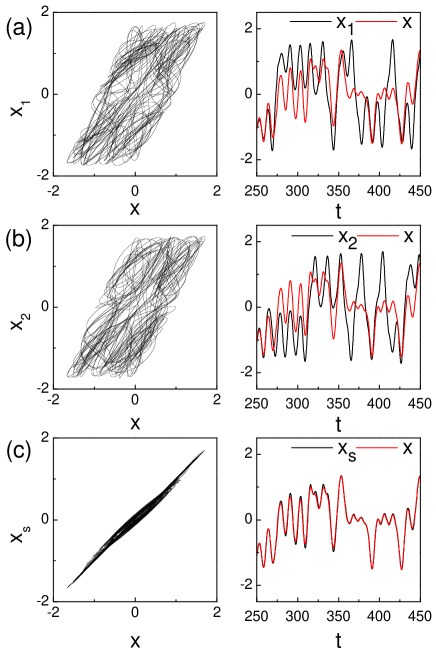
Figure 1: Output of the Gauthier-Bienfang nonlinear system with addition of a linear combination of 2-solution coupling. (a) $x_{1}\times x$; (b) $x_{2}\times x$; (c) $x_{s}=\frac{(x_{1}+x_{2})}{2}\times x$. Left: synchronization analysis; Right: temporal series.

We show in Figure 1(a,b) the graphs $x\times x_{1}$ and $x\times x_{2}$, as well as the temporal series for $x$, $x_{1}$ and $x_{2}$. Clearly, the system does not synchronize with any of the two individual components, with both phase and amplitude uncorrelated. These comparative trajectories and temporal series are shown in Figure 1(c) for the component $x_{s}=(x_{1}+x_{2})/2$ of the sum of the two drive variables $x_{1}$ and $x_{2}$. The component $x$ of the response oscillator synchronizes with the component $x_{s}$ of the weighted linear sum signal.

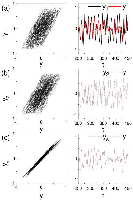
Figure 2: Output of the Gauthier-Bienfang nonlinear system with addition of a linear combination of 2-solution coupling. (a) $y_{1}\times y$; (b) $y_{2}\times y$; (c) $y_{s}=\frac{(y_{1}+y_{2})}{2}\times y$. Left: synchronization analysis; Right: temporal series.

Figures 2 and 3 exhibit graphs $y\times y_{n}$ and $z\times z_{n}$ for $n=1,2$ and temporal series for the components of the drive and receiving systems. The strong synchronization between $\bf{X}$ and $\bf{X_{s}}$ is displayed in all the components synchronization curves, $\bf{X}\times\bf{X_{s}}$, as well as in the temporal series $\bf{X}(t)$ and $\bf{X_{s}}(t)$. Comparing the solution variables $\mathbf{X}_{n}(t)$ $(n=1,2)$ to those of the oscillator, $\bf{X}(t)$, we do not observe any regular relation of phase between the solution and individual variables (Figs. 1-3 (a,b)), but only with the sum of the solutions used to define $\bf{X_{s}}$(Figs. 1-3 (c)).

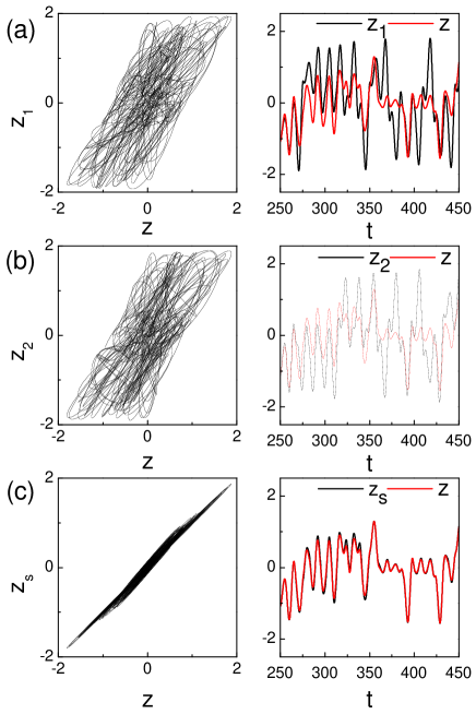
Figure 3: Output of the Gauthier-Bienfang nonlinear system with addition of a linear combination of 2-solution coupling. (a) $z_{1}\times z$; (b) $z_{2}\times z$; (c) $z_{s}=\frac{(z_{1}+z_{2})}{2}\times z$. Left: synchronization analysis; Right: temporal series.

We have investigated the behaviour of the solution of equation (2) as a function of the number $N$ of solutions of Eq.(1) composing $\bf{X}_{s}$. For simplification purposes we consider $c_{n}=c$ $(n=1,2,....N)$. We define the vector $\bf{X}_{\bot}=(\bf{X}_{s}-\bf{X})$ and show in Figure 4 the behavior of the distance $|\bf{X}_{\bot}|$ mod as a function of the coupling coefficient $c$, that evidences the convergence to synchronization for a large number of added solutions. Figure 4(a) exhibits $|\mathbf{X}_{\bot}|_{max}$, the maximum value of $|\mathbf{X}_{\bot}|$ in the temporal series, which is more sensitive to local instability, and Figure 4(b) displays $|\mathbf{X}_{\bot}|_{rms}$, the average value of $|\mathbf{X}_{\bot}|$ in the temporal series, as a measure of the global stability of solution $\bf{X}$. A monotonic convergence of $|\mathbf{X}_{\bot}|$ to zero is observed as the number of solutions added into $\bf{X}_{s}$ is increased.

The decreasing of both $|\mathbf{X}_{\bot}|_{max}$ and $|\mathbf{X}_{\bot}|_{rms}$ as $N$ increases confirms the behaviour observed in the graphs $\frac{1}{2}(\mathbf{X}_{1}+\mathbf{X}_{2})\times\bf{X}$ of Figs 1-3(c) in the case of two solutions only: the convergence of $\bf{X}$ toward $\bf{X_{s}}$ improves as the number of solutions in $\bf{X_{s}}$ increases. We have likewise applied this technique to Lorenz and Rössler systems. Both also converge to the solution-sum, yet Rössler shows a slower convergence for the $z$-variable with the number of solutions.

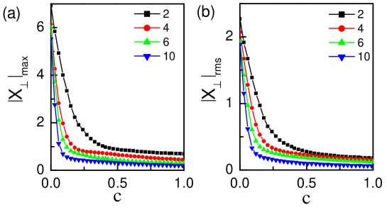
Figure 4: Measure of the convergence of the oscillator trajectory to a sum signal. (a) $|\mathbf{X}_{\bot}|_{max}$ and (b) $|\mathbf{X}_{\bot}|_{rms}$, for the sum of: 2 (black squares), 4 (red circles), 6 (green up triangle), and 10 (blue down triangle) solutions.

III Conclusion

We showed that is possible to create a state of coherence in a classical, chaotic system. The non-linear system oscillates, following trajectories that are not a simple solution of the system equations but a linear combination of solutions. The increased sensitivity of nonlinear systems to a high number of solutions, even when only a partial information is transmitted through one or few variables, gives an insight into processes where a large number of inputs determine a single output, as occurs in complex networks such as neural systems.