Asymptotic Performance of Box-RLS Decoders under Imperfect CSI with Optimized Resource Allocation

Abstract

This paper considers the problem of symbol detection in massive multiple-input multiple-output (MIMO) wireless communication systems. We consider hard-thresholding preceded by two variants of the regularized least squares (RLS) decoder; namely the unconstrained RLS and the RLS with box constraint. For all schemes, we focus on the evaluation of the mean squared error (MSE) and the symbol error probability (SEP) for $M$-ary pulse amplitude modulation ($M$-PAM) symbols transmitted over a massive MIMO system when the channel is estimated using linear minimum mean squared error (LMMSE) estimator. Under such circumstances, the channel estimation error is Gaussian which allows for the use of the convex Gaussian min-max theorem (CGMT) to derive asymptotic approximations for the MSE and SEP when the system dimensions and the coherence duration grow large with the same pace. The obtained expressions are then leveraged to derive the optimal power distribution between pilot and data under a total transmit energy constraint. In addition, we derive an asymptotic approximation of the goodput for all schemes which is then used to jointly optimize the number of training symbols and their associated power. Numerical results are presented to support the accuracy of the theoretical results.

I Introduction

The use of multiple-input multiple-output (MIMO) systems has been recognized as an efficient technology to meet the ever-increasing demand in spectral efficiency. It is indeed known since the early works of Telatar [2] and Foshini [3] that the mutual information scales with the minimum of the number of transmit and receive antennas. In practice, however, the spectral efficiency of a wireless link depends not only on how many antennas are deployed at the transmit and receive sides but also on the channel estimation accuracy, the detection procedure as well as the distribution of the power resources, all of which have a direct bearing on the end-to-end signal-to-noise-ratio. At the receiver side, accurate channel estimation and symbol detection are crucial to reap the gains promised by the additional degrees of freedom offered by MIMO systems. Channel estimation is performed by allocating a training period during which the transmitter sends known pilot symbols to the receiver for it to acquire an estimate of the channel state information (CSI). During the data transmission phase, this estimate is leveraged by the receiver to equalize the channel and recover the data symbols. It is worth mentioning that it is important for the success of the data recovery step to acquire accurate channel estimates because otherwise the error in the channel estimation would propagate to the symbol recovery, crippling the overall performance even under state-of-the-art detection strategies. Resource allocation in terms of power and time is also an essential part of the design of wireless systems. Increasing the duration of the transmitted pilot sequence would lead to enhanced channel estimation quality but at the cost of spectral efficiency losses since less time is spent to transmit useful data. Moreover, as the total power allocated to data and training transmission is fixed, we cannot increase the power allocated to data without affecting the channel accuracy estimation and vice versa.

The problem of finding optimal power allocation between pilot and data has received a lot of attention over the last decades. It has been applied to different contexts with the aim of realizing various communication objectives. In [4], [5] and [6], the authors proposed power designs that optimizes bounds on the average channel capacity. A different line of research works in [7, 8, 9, 10] considered the post-equalization signal to interference and noise ratio as a target metric to determine the optimal power allocation. Depending on the application at hand, different other metrics such as the bit error rate (BER) [11, 12], the symbol error rate (SER) [13], mean squared error (MSE)-related indexes [14, 15], max-min fairness utilities [16] or bounds on the received signal-to-noise ratio [17] have been used in several existing papers. Of interest in these works are a wide range of contexts including classical MIMO systems [4], mutli-carrier systems [18, 19, 20, 21, 22, 23], amplify-and-forward relaying [11], cognitive radio systems [24] and very recently massive MIMO systems in both single-cell [25] and multi-user multi-cell settings [16, 26, 27, 14, 28].

Most of the aforementioned works, despite looking at the power allocation problem from different angles, present the common denominator of relying on linear receivers and optimizing some related performance metrics. To achieve optimal performance, it is well known that non-linear detectors are required, but they are often not implemented as they require a prohibitively high computation complexity. In this work, we consider optimization of the power allocation of a non-linear decoder coined Box-RLS decoder, the idea behind which has been proposed in [29, 30] and earlier in [31]. As explained in [31], this decoder is rooted in the formulation of the maximum-likelihood (ML) problem. At the one hand, the ML decoder is known to be NP-hard since its solution is constrained to belong to a finite discrete set, at the other hand, the Least Square (LS) decoder or its regularized version referred to as Regularized Least Squares (RLS) decoder [32] are linear detectors, obtained by solving the unconstrained ML problem. The Box-RLS decoder falls between the ML and the RLS decoders in that the solution is constrained to lie within a closed convex-set. As a consequence, unlike the RLS decoder, the solution of the Box-RLS cannot be expressed in closed-form but is numerically computed using standard convex-optimization tools. Both the RLS and Box-RLS decoders are more computationally efficient than the ML decoder. Besides they are also shown to outperform many heuristic algorithms such as zero-forcing (ZF), successive interference cancellation and decision-feedback, [29, 30, 31]. Performance analysis of the Box-RLS has been carried out in [29], [30] but these studies assume unrealistic scenarios in which the channel is perfectly known and do not address the problem of power allocation. To fill this gap, this work addresses the problem of finding optimal power allocation between pilots and data for RLS and Box-RLS under a fixed total power constraint and when the channel is estimated using the linear minimum mean square error estimator (LMMSE). Particularly, we derive sharp characterization of the MSE and symbol error probability (SEP) for the RLS and Box-RLS decoders under $M$-ary pulse amplitude modulation ($M$-PAM) when assuming that the symbol is recovered by hard-thresholding the output of RLS and Box-RLS decoders. Our analysis, based on the assumption that the MIMO channel and the noise are independent and follow standard Gaussian distributions, builds upon the CGMT framework put forth in [33, 34, 35]. As compared to previous works dealing with the use of CGMT in high-dimensional regression problems, our consideration of imperfect CSI poses technical challenges towards assessing the performance of the Box-RLS. Particularly, contrary to previous studies, the application of the CGMT in the asymptotic regime leads to a non-convex optimization problem; the uniqueness of its solution which is an important step in the analysis becomes thus extremely challenging. This required us to develop new techniques to break these difficulties, which while being accommodated to this specific scenario, may be of independent interest. We refer the interested reader to Appendix B devoted to the detailed proofs of our main results.

To summarize, the main contributions of this work can be listed as follows:

1. We derive sharp characterizations of the MSE, SEP and goodput expressions for the RLS, LS and Box-RLS under imperfect CSI. Our expressions shed light on interesting relationships between MSE and SEP for $M$-PAM modulation and under imperfect CSI.

2. We determine the optimal power allocation between training and data symbols when SEP or MSE are used as target criteria.

3. We optimize the power and the number of pilot symbols to maximize the goodput for all studied decoders.

To the best of our knowledge, none of the above was previously derived for the $M$-PAM case in the presence of imperfect CSI.

I-A Paper Organization

This paper is organized as follows. The system model is presented in Section II. In Section III, we discuss channel estimation, the properties of the estimator and the channel estimation error, as well as symbol estimation. The MSE/SEP of symbol estimation is derived in Section IV by applying the CGMT. These expressions are then validated through an assortment of numerical results and leveraged to find optimal power strategies in Section V. The key ingredient of the analysis which is the CGMT is reviewed in Appendix A. The proofs for the derived MSE and SEP are presented in Appendix B and Appendix C for the Boxed RLS and un-boxed RLS, respectively.

I-B Notations

Scalars are denoted by lower-case letters (e.g., $\alpha$), column vectors are represented by boldface lowercase letters (e.g., ${\bf x}$), whereas matrices are denoted by boldface upper-case letters (e.g., ${\bf X}$). The notations $(\cdot)^{T}$ and $(\cdot)^{-1}$ denote the transpose and inversion operators, respectively. The $j$-th element of vector ${\bf x}$ will be denoted by ${x}_{j}$. The symbol ${\bf I}_{N}$ is used to represent the identity matrix of dimension $N\times N$. We use the standard notation $\mathbb{P}[\cdot]$ and $\mathbb{E}[\cdot]$ to denote probability and expectation. We write $X\thicksim p_{X}$ to denote that a random variable $X$ has a probability density function (pdf) $p_{X}$. In particular, $G\thicksim\mathcal{N}(\mu,\sigma^{2})$ implies that $G$ has a Gaussian (normal) distribution of mean $\mu$ and variance $\sigma^{2}$. $p(x)=\frac{1}{\sqrt{2\pi}}e^{\frac{-x^{2}}{2}}$ and $Q(x)=\frac{1}{\sqrt{2\pi}}\int_{x}^{\infty}e^{-t^{2}/2}{\rm{d}}t$ denote the pdf of a standard normal distribution and its associated $Q$-function respectively. Finally, $\|\cdot\|$ indicates the Euclidean norm (i.e., the $\ell_{2}$-norm) of a vector and $\|\cdot\|_{\infty}$ represents its $\ell_{\infty}$-norm.

TABLE I: Summary of Main Variables

Symbol	Meaning
$T_{\tiny{p}}$	number of pilot symbols
$T_{d}$	number of data symbols
$T$	total number of symbols
$M$	size of the PAM signal
$\mathcal{E}$	average power of non-normalized $M$-PAM signal
$\rho_{p}$	average training power
$\rho_{d}$	average data power
$\rho$	average received power per receive antenna
$\rho_{\text{eff}}$	effective SNR
$\alpha$	data power ratio
$K$	Number of transmit (Tx) antennas
$N$	Number of receive (Rx) antennas
$\delta$	ratio of Rx to Tx antennas $N/K$
$\lambda$	regularization coefficient
$t$	box-constraint threshold
${\bf H}$	channel matrix
$\widehat{{\bf H}}$	estimated channel matrix
$\Delta$	channel estimation error matrix
$\sigma_{{\Delta}}^{2}$	variance of error matrix
$\sigma_{{\hat{H}}}^{2}$	variance of estimated channel matrix
${\bf X}_{p}$	pilot symbols matrix
${\bf x}_{0}$	transmitted data symbol vector
$\widehat{{\bf x}}$	estimated data symbol vector
${\bf y}$	received data symbol vector
${\bf z}$	noise vector

II System Model

We consider a flat block-fading massive MIMO system with $K$ transmitter antennas and $N$ receiver antennas. The transmission consists of $T$ symbols that occur in a time interval within which the channel is assumed to be static. A number $T_{p}$ pilot symbols (for channel estimation) occupy the first part of the transmission interval with power, $\rho_{p}$. The remaining part is devoted for transmitting $T_{d}=T-T_{p}$ data symbols with power, $\rho_{{d}}$. Figure 1 illustrates the system model. It implies from conservation of time and energy that:

$$\rho_{p}T_{p}+\rho_{{d}}T_{d}=\rho T,$$ (1)

where $\rho$ is the expected average power. Alternatively, we have $\rho_{d}T_{d}=\alpha\rho T$, where $\alpha\in(0,1)$ is the ratio of the power allocated to the data so that

$$\rho_{p}T_{p}=(1-\alpha)\rho T.$$ (2)

The received signal model for the data transmission phase is given by

$${\bf y}=\sqrt{\frac{\rho_{d}}{K}}{\bf H}{\bf x}_{0}+{\bf z},$$ (3)

where ${\bf y}\in\mathbb{R}^{N}$ is the received data symbol vector, ${\bf x}_{0}\in\mathbb{R}^{K}$ is the transmitted data symbol vector, ${\bf H}\in\mathbb{R}^{N\times K}$ is a channel matrix with i.i.d. Gaussian elements $h_{ij}\thicksim\mathcal{N}\left(0,1\right)$, and ${\bf z}\in\mathbb{R}^{N}$ stands for the additive Gaussian noise at the receiver with i.i.d. elements of mean $0$ and variance 1. It is assumed that ${\bf x}_{0}$ has i.i.d. $M$-PAM symbols normalized to have unit variance ($\mathbb{E}[{\bf x}_{0}{\bf x}_{0}^{T}]={\bf I}_{K}$), such that each transmit antenna sends a data symbol $x_{0,j}$ that takes values (with equal probability $1/M$) in the set:

$$x_{0,j}\in\mathcal{C}:=\bigg{\{}\pm\frac{1}{\sqrt{\mathcal{E}}},\pm\frac{3}{\sqrt{\mathcal{E}}},\cdots,\pm\frac{(M-1)}{\sqrt{\mathcal{E}}}\bigg{\}},j=1,2,\cdots,K,$$ (4)

where $\mathcal{E}=\frac{M^{2}-1}{3}$ is the average power of the non-normalized $M$-PAM signal, $M=2^{b}$ being the modulation order and $b$ the number of bits carried by each symbol.

As the channel matrix ${\bf H}$ is unknown to the receiver, a training phase during which the transmitter sends $T_{{p}}\geq K$ pilot symbols is dedicated. The received signals corresponding to this phase can be modeled as

$${\bf Y}_{p}=\sqrt{\frac{\rho_{p}}{K}}{\bf H}{\bf X}_{p}+{\bf Z}_{p},$$ (5)

where ${\bf Y}_{p}\in\mathbb{R}^{N\times T_{p}}$ is the received signal matrix, ${\bf X}_{p}\in\mathbb{R}^{K\times T_{p}}$ is the matrix of transmitted pilot symbols, and ${\bf Z}_{p}\in\mathbb{R}^{N\times T_{p}}$ stands for the additive Gaussian noise with $\mathbb{E}[{\bf Z}_{{p}}{\bf Z}_{{p}}^{T}]=T_{{p}}{\bf I}_{N}$.

For the reader convenience, we summarize in Table I the notation symbols of the parameters used in this paper.

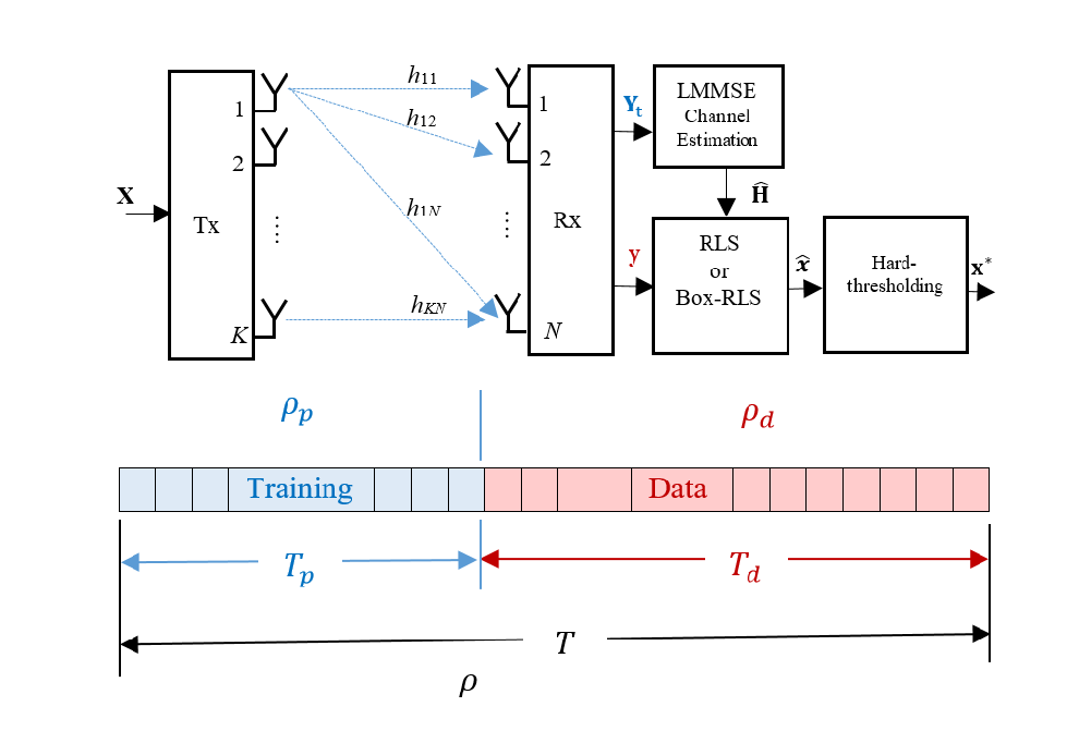
Figure 1: Massive MIMO system with training-based transmission.

III MIMO Symbols Detection under LMMSE Channel Estimation

III-A LMMSE Channel Estimation

Based on the knowledge of ${\bf Y}_{p}$ from (5), the LMMSE channel estimate is given by [36]

$$\widehat{{\bf H}} =\sqrt{\frac{K}{\rho_{p}}}{\bf Y}_{p}{\bf X}_{{p}}^{T}\left(\frac{K}{\rho_{p}}{\bf I}_{K}+{\bf X}_{{p}}{\bf X}_{{p}}^{T}\right)^{-1},$$

$$={\bf H}-\hbox{\boldmath$\Delta$},$$ (6)

where $\Delta$ is the zero-mean channel estimation error matrix, which is independent of $\widehat{{\bf H}}$, as per the orthogonality principle of the LMMSE estimation [4], [36]. For MIMO channels with i.i.d. entries, it has been proved that the optimal ${\bf X}_{p}$ that minimizes the estimation mean squared error under a total power constraint satifies [4]

$${\bf X}_{p}{\bf X}_{{p}}^{T}=T_{p}{\bf I}_{K}.$$ (7)

For the above condition to hold, the number of training symbols should be greater than or equal to $K$. Moreover, under (7), the channel estimate $\widehat{{\bf H}}$ has i.i.d. zero-mean Gaussian entries with mean $0$ and variance $\sigma_{{\hat{H}}}^{2}=1-\sigma_{{\Delta}}^{2}$ [4], with

$$\sigma_{{\Delta}}^{2}=\frac{1}{1+\frac{\rho_{p}}{K}T_{p}},$$ (8)

being the variance of each element in $\Delta$. It appears from (8) that channel estimation error decreases with the pilot energy given by $\rho_{p}T_{p}$.

III-B Symbol Detection under Imperfect Channel Estimation

With the channel estimate $\widehat{{\bf H}}$ at hand, the receiver can proceed to the recovery of the transmitted symbols. The optimal decoder which minimizes the probability of error is the maximum likelihood (ML) decoder under perfect channel knowledge which is given by:

$$\widehat{{\bf x}}_{\text{\tiny{ML}}}=\underset{{{\bf x}\in\mathcal{C}^{{K}}}}{\operatorname*{arg\,min}}\big{\|}{\bf y}-\sqrt{\frac{\rho_{d}}{K}}{\bf H}{\bf x}\big{\|}^{2}.$$ (9)

As can be seen, the ML decoder involves a combinatorial optimization problem. It presents thus a prohibitively high computational complexity, especially when the system dimensions become large as envisioned by current communication systems. To overcome this issue, suboptimal strategies that require less computational complexity are in general used. They often proceed in two steps. First, a real-valued approximation of the transmitted symbol is obtained. This estimate is then hard-thresholded in a second step to produce the final estimate. In this work, the focus is on the regularized least squares (RLS) and the Box-regularized least squares (Box-RLS) decoders.

The RLS decoder is based on regularizing the cost in (9) and relaxing the finite-alphabet constraint, thus leading to:

$$\widehat{{\bf x}} =\operatorname*{arg\,min}_{{\bf x}\in\mathbb{R}^{{K}}}\|{\bf y}-\sqrt{\frac{\rho_{d}}{K}}\widehat{{\bf H}}{\bf x}\|^{2}+\lambda\rho_{d}\|{\bf x}\|^{2},$$ (10a)

$$=({\bf A}^{T}{\bf A}+{\lambda}\rho_{d}{\bf I}_{K})^{-1}{\bf A}^{T}{\bf y},$$ (10b)

$${x}_{j}^{*} =\operatorname*{arg\,min}_{s\in\mathcal{C}}\bigg{|}\frac{\widehat{x}_{j}}{B}-s\bigg{|},j=1,2,\cdots,K,$$ (10c)

where $\lambda\geq 0$ is the regularization coefficient, ${\bf A}=\sqrt{\frac{\rho_{d}}{K}}\widehat{{\bf H}}$ and $B$ is a normalization constant, the value of which will be suggested from our analysis so as to remove the bias of the decoder [37] . Note that the optimization in (10c) simply selects the symbol value $s$ that is closest to the solution $\frac{\widehat{x}_{j}}{B}$ among a total of $M$ possible choices. As can be seen from (10b), the elements of the solution $\widehat{{\bf x}}$ may take large values in high-noise conditions or poor channel estimation scenarios. This motivates the Box-RLS decoder [38, 31, 39] given by

$$\widehat{{\bf x}} =\operatorname*{arg\,min}_{\|{\bf x}\|_{\infty}\leq t}\|{\bf y}-\sqrt{\frac{\rho_{d}}{K}}\widehat{{\bf H}}{\bf x}\|^{2}+\lambda\rho_{d}\|{\bf x}\|^{2},$$ (11a)

$${x}_{j}^{*}=\operatorname*{arg\,min}_{s\in\mathcal{C}}\bigg{|}\frac{\widehat{x}_{j}}{B}-s\bigg{|},j=1,2,\cdots,K,$$ (11b)

which is based on relaxing the finite-alphabet constraint to the convex constraint ${\bf x}\in[-t,t]^{K}$, where $t$ is a fixed threshold that can be optimally tailored according to the propagation scenario.

III-C Performance Metrics

This work considers the performance evaluation of the RLS and the Box-RLS decoders in terms of three different performance metrics, which are:

Mean Squared Error: A natural and heavily used measure of performance is the reconstruction mean squared error (MSE), which measures the deviation of $\widehat{{\bf x}}$ from the true signal ${\bf x}_{0}$. This assesses the performance of the first step of the decoding algorithms. Formally, the MSE is defined as

$${\rm{MSE}}:=\frac{1}{K}\|\widehat{{\bf x}}-{\bf x}_{0}\|^{2}.$$ (12)

Symbol Error Probability: The symbol error rate (SER) characterizes the performance of the detection process and is defined as:

$${\rm{SER}}:=\frac{1}{K}\sum_{j=1}^{K}{\bf 1}_{\{{x}^{*}_{j}\neq x_{0,j}\}},$$ (13)

where ${\bf 1}_{\{\cdot\}}$ indicates the indicator function.
In relation to the SER is the symbol error probability (SEP) which is defined as the expectation of the SER averaged over the noise, the channel and the constellation. Formally, the symbol error probability denoted by ${\rm SEP}$ is given by:

$${\rm SEP}:=\mathbb{E}[{\rm SER}]=\frac{1}{K}\sum_{j=1}^{K}\mathbb{P}\left[{x}^{*}_{j}\neq x_{0,j}\right].$$ (14)

Goodput: The goodput is a performance measure that accounts for the amount of useful data transmitted, divided by the time it takes to successfully transmit it. The amount of data considered excludes protocol overhead bits as well as retransmitted data packets [40]. In our context, it can be defined as

$$G:=\left(\frac{T-T_{p}}{T}\right)\left(1-{\rm SEP}\right).$$ (15)

Goodput and throughput are connected performance parameters in that the throughput can be obtained by simply dividing the goodput by the data transmission rate.

IV Analysis of the Mean Squared Error (MSE) and Symbol-Error Probability (SEP)

In this section, we derive asymptotic expressions of the MSE and SEP for the RLS and Box-RLS decoders. Particularly, we show that these metrics can be approximated by deterministic quantities that involve the power and time devoted for data and training transmissions. Our analysis builds upon the CGMT framework. For the RLS decoder, the same results could have been obtained using tools from random matrix theory as the decoder possesses a closed-form expression. However, since the use of the CGMT framework is more adapted to the Box-RLS decoder that cannot be expressed in closed-form, we rely in this work on the CGMT framework for both decoders for the sake of a unified presentation.

Prior to stating our main results, we shall introduce the following assumptions which describe the considered growth rate regime:

IV-A Technical Assumptions

Assumption 1.

We consider the asymptotic regime in which the system dimensions $K$ and $N$ grow simultaneously to infinity at a fixed ratio

$$\delta:=\frac{N}{K}\in(0,\infty).$$

Assumption 2.

We assume a fixed normalized coherence interval

$$\tau:=\frac{T}{K}\in(1,\infty).$$

and that the pilot and data symbols grow proportionally with $K$, where:

$$\tau_{{p}}:=\frac{T_{{p}}}{K}\in[1,\infty),$$

and

$$\tau_{{d}}:=\frac{T_{{d}}}{K},$$

are fixed and denote the normalized number of pilot and data symbols, respectively.

In the sequel, we leverage the statistical distribution of the channel and the channel estimate as well as the asymptotic regime specified in Assumption 1 and 2 to provide asymptotic approximations of the MSE and SEP for RLS and Box-RLS. We use the standard notation ${\rm{plim}}_{n\to\infty}\ X_{n}=X$ to denote that a sequence of random variables $X_{n}$ converges in probability towards a constant $X$.

IV-B MSE and SEP Analysis for RLS

We provide herein asymptotic approximations of the MSE and SEP for RLS under imperfect channel state information. The derived closed form expressions are given in Theorem 1, and Theorem 2 while the proof is given in Appendix C.

Theorem 1.

(MSE for RLS): Fix $\lambda>0$, $\delta>0$, and let $\widehat{{\bf x}}$ be a minimizer of the RLS problem in (10a). Define

$$\Upsilon(\lambda,\delta)=\frac{-(\delta-\frac{\lambda}{\sigma_{{\hat{H}}}^{2}}-1)+\sqrt{(\delta-\frac{\lambda}{\sigma_{{\hat{H}}}^{2}}-1)^{2}+4\frac{\lambda}{\sigma_{{\hat{H}}}^{2}}\delta}}{2\delta},$$

and

$$\theta_{\star}=\sqrt{\frac{\rho_{d}\sigma_{{\hat{H}}}^{2}\left(\frac{\Upsilon(\lambda,\delta)}{1+\Upsilon(\lambda,\delta)}\right)^{2}+\rho_{d}\sigma_{{\Delta}}^{2}+1}{\delta-\frac{1}{(1+\Upsilon(\lambda,\delta))^{2}}}}.$$

Then, under Assumption 1 and Assumption 2, it holds:

$$\underset{K\to\infty}{{\rm{plim}}}{\rm{MSE}}=\frac{1}{\rho_{d}\sigma_{{\hat{H}}}^{2}}\biggl{(}\delta\theta_{\star}^{2}-\rho_{d}\sigma_{{\Delta}}^{2}-1\biggr{)},$$ (16)

Proof.

The proof of Theorem 1 is given in Appendix C. ∎

It is worth mentioning that the above formula is not restricted to ${\bf x}_{0}$ belonging to $M$-PAM constellation and is valid for ${\bf x}_{0}$ from any distribution provided that ${\bf x}_{0}$ is normalized to have unit-variance. However, assuming that ${\bf x}_{0}$ is drawn from $M$-PAM constellations, the SEP can be approximated as:

Theorem 2.

(SEP of RLS): Under the same setting of Theorem 1, the SEP under $M$-PAM modulation of the RLS decoder employing the normalization constant

$$B=\frac{\sigma_{{\hat{H}}}^{2}\frac{\beta_{\star}}{\theta_{\star}}}{\sigma_{{\hat{H}}}^{2}\frac{\beta_{\star}}{\theta_{\star}}+2\lambda},$$

with $\beta_{\star}=\frac{2\lambda\theta_{\star}}{\sigma_{{\hat{H}}}^{2}\Upsilon(\lambda,\delta)}$, converges to:

$$\underset{K\to\infty}{{\rm{plim}}}{\rm{SEP}}=\widetilde{\rm{SEP}}_{\rm RLS},$$ (17)

where

$$\widetilde{\rm{SEP}}_{\rm RLS}=2\bigg{(}1-\frac{1}{M}\bigg{)}Q\biggl{(}\frac{\sqrt{\rho_{{d}}\sigma_{{\hat{H}}}^{2}}}{\sqrt{\mathcal{E}}\theta_{\star}}\biggr{)}.$$ (18)

where $\theta_{\star}$ is defined in Theorem 1.

Proof.

A sketch of the proof is provided in Appendix C. ∎

Before proceeding further, we validate the approximations provided in Theorem 16 and Theorem 2. To this end, we report in Figure 2 and 3 the MSE and SEP for the RLS decoder when $K=400,\delta=1.2,T_{p}=456,T=1000$, $\alpha=0.5$ and $M=2$ (corresponding to Binary Phase Shift Keying (BPSK) modulation), as a function of the average power $\rho$. As seen, the simulation results, averaged over 500 realizations of the channel, show a perfect agreement with the theoretical results.

Figure 2: MSE performance of both RLS and Box-RLS decoders.

Figure 3: Symbol error probability of both RLS and Box-RLS decoders.

Corollary 1.

(Optimal regularization coefficient for RLS in MSE and SEP senses): Let $\lambda_{\star}$ denote the optimal regularization coefficient that minimizes the limit in (16) or in (17). Then,

$$\lambda_{\star}=\frac{1}{\rho_{d}}+\sigma_{{\Delta}}^{2}.$$ (19)

Proof.

Note that in both (16) and (17), the regularization coefficient $\lambda$ appears through $\theta_{\star}$ only. Then, $\lambda_{\star}={\operatorname*{arg\,min}}_{\lambda\geq 0}\theta_{\star}$. Taking the derivative of $\theta_{\star}$ with respect to $\lambda$, setting it to zero and solving completes the proof of the corollary. ∎

Remark 1.

It is worth mentioning that the optimal regularization coefficient in (19) minimizes both the MSE and SEP. Moreover, it can be written in terms of the so called effective SNR of the system [4] as $\lambda_{\star}=\frac{\sigma_{{\hat{H}}}^{2}}{\rho_{\text{eff}}}$, where

$$\rho_{\text{eff}}:=\frac{\rho_{d}\sigma_{{\hat{H}}}^{2}}{1+\rho_{d}\sigma_{{\Delta}}^{2}}.$$ (20)

Remark 2.

In Appendix H, we show that the RLS detector with optimal regularization coefficient is equivalent to the LMMSE detector. The later is known by definition to minimize the MSE, but it turns out according to Corollary 1 that it also minimizes the asymptotic SEP among all other choices of $\lambda$. In the perfect CSI case, $\sigma_{{\Delta}}^{2}=0$, hence the optimal regularization coefficient becomes ${\lambda}_{\star}=\frac{1}{\rho_{d}}$ which is clearly equivalent to the LMMSE decoder. This shows that in both perfect and imperfect settings, the RLS with optimal regularization coefficient turns out to be the LMMSE detector. Such a finding is appealing due to the fundamental importance of the LMMSE decoder in many applications.

IV-C MSE and SEP Analysis for Box-RLS

In this subsection, we study the asymptotic performance of the Box-RLS decoder in terms of the MSE and SEP. We first present the MSE results in the following theorem.

Theorem 3.

(MSE of Box-RLS): Fix $\lambda>0$, $\delta>0$, and let $\widehat{{\bf x}}$ be a minimizer of the Box-RLS problem in (11a). Let $\beta_{\star}$ and $\theta_{\star}$ be the unique solutions in $\beta$ and $\theta$ to the following max-min problem:

$$\sup_{\beta>0}\min_{\theta\geq 0} \ D(\theta,\beta):=\frac{\beta\delta\theta}{2}+\frac{\beta}{2\theta}(1+\rho_{{d}})-\frac{\beta^{2}}{4}+\frac{1}{M}\sum_{i=\pm 1,\pm 3,\cdots,\pm(M-1)}\Psi(\theta,\beta;i),$$ (21)

with

$$\Psi(\theta,\beta;i):= t\big{(}c_{i}Q(-\ell_{i})+d_{i}Q(\mu_{i})\big{)}-\beta\sqrt{\rho_{{d}}\sigma_{\hat{{H}}}^{2}}t\big{(}p(\ell_{i})+p(\mu_{i})\big{)}$$

$$- \frac{\beta^{2}}{{2\rho_{{d}}\sigma_{\hat{{H}}}^{2}\frac{\beta}{\theta}}+4\lambda\rho_{{d}}}\int_{\ell_{i}}^{\mu_{i}}\bigg{(}\frac{\rho_{{d}}\sigma_{\hat{{H}}}^{2}i}{\sqrt{\mathcal{E}\theta}}+\sqrt{\rho_{{d}}\sigma_{\hat{{H}}}^{2}}h\bigg{)}^{2}p(h){\rm{d}}h,$$ (22)

where $\ell_{i}=-t(\frac{\sqrt{\rho_{{d}}\sigma_{\hat{{H}}}^{2}}}{\theta}+\frac{2\lambda\rho_{d}}{\sqrt{\rho_{{d}}\sigma_{\hat{{H}}}^{2}}\beta})-\frac{\sqrt{\rho_{{d}}\sigma_{\hat{{H}}}^{2}}i}{\theta\sqrt{\mathcal{E}}}$, $\mu_{i}=t(\frac{\sqrt{\rho_{{d}}\sigma_{\hat{{H}}}^{2}}}{\theta}+\frac{2\lambda\rho_{d}}{\sqrt{\rho_{{d}}\sigma_{\hat{{H}}}^{2}}\beta})-\frac{\sqrt{\rho_{{d}}\sigma_{\hat{{H}}}^{2}}i}{\theta\sqrt{\mathcal{E}}}$, $c_{i}=\frac{-\beta\sqrt{\rho_{{d}}\sigma_{\hat{{H}}}^{2}}}{2}\ell_{i}+\frac{\beta{\rho_{{d}}\sigma_{\hat{{H}}}^{2}}i}{2\theta\sqrt{\mathcal{E}}}$, and $d_{i}=\frac{\beta\sqrt{\rho_{{d}}\sigma_{\hat{{H}}}^{2}}}{2}\mu_{i}-\frac{\beta{\rho_{{d}}\sigma_{\hat{{H}}}^{2}}i}{2\theta\sqrt{\mathcal{E}}}$. Then, under Assumption 1 and Assumption 2, it holds:

$$\underset{K\to\infty}{{\rm{plim}}}{\rm{MSE}}=\frac{1}{\rho_{d}\sigma_{{\hat{H}}}^{2}}\biggl{(}\delta\theta_{\star}^{2}-\rho_{d}\sigma_{{\Delta}}^{2}-1\biggr{)},$$ (23)

Proof.

The proof of this theorem is deferred to Appendix B. ∎

Remark 3.

It is worth mentioning that contrary to previous works based on the framework of the CGMT, the optimization problem in (21) which resulted from the asymptotic analysis is not convex-concave in the variables $\theta$ and $\beta$. Indeed, it is concave in $\beta$ but not convex in $\theta$. This poses a major challenge to prove the uniqueness of the solutions in $\theta$ of (21), which is a crucial step that is required to ensure convergence results. The reader can refer to Appendix B for more details of the technical arguments developed to show the uniqueness of the solutions of (21).

Remark 4.

If the optimal values $\theta_{\star}$ and $\beta_{\star}$ are strictly positive, then they satisfy the following first-order stationarity conditions:

$$\frac{\partial D(\theta,\beta)}{\partial\theta}=0,$$

$$\frac{\partial D(\theta,\beta)}{\partial\beta}=0.$$

which can be exploited in practice to facilitate their numerical evaluation.

The following theorem provides the asymptotic expression of the SEP for the Box-RLS decoder.

Theorem 4.

(SEP for Box-RLS): Under the same settings of Theorem 3, assuming that the Box-RLS decoder uses a normalization constant given by $B=\frac{\sigma_{\hat{{H}}}^{2}\frac{\beta_{\star}}{\theta_{\star}}}{\sigma_{\hat{{H}}}^{2}\frac{\beta_{\star}}{\theta_{\star}}+2\lambda}$ where $\beta_{\star}$ is the solution to (21) in $\beta$, and that $t\notin\left\{\frac{Bi}{\sqrt{\mathcal{E}}},i=1,3\cdots,M-1\right\}$, it holds that:

$$\underset{K\to\infty}{{\rm{plim}}}{\rm SEP}=\widetilde{{\rm SEP}}_{\text{\tiny Box-RLS}},$$

where $\widetilde{\rm{SEP}}_{\text{\tiny Box-RLS}}$ is given in (24).

$$\widetilde{\rm SEP}_{\text{\tiny Box-RLS}} =\frac{4}{M}\sum_{i=1,3,\dots,M-3}{\bf 1}_{\{\frac{t}{B}\geq\frac{i+1}{\sqrt{\mathcal{E}}}\}}Q\left(\frac{\sqrt{\rho_{{d}}\sigma_{\hat{{H}}}^{2}}}{\sqrt{\mathcal{E}}\theta_{\star}}\right)+\frac{2}{M}\sum_{i=1,3,\cdots,M-3}\left\{{\bf 1}_{\{\frac{i-1}{\sqrt{\mathcal{E}}}\leq\frac{t}{B}\leq\frac{i+1}{\sqrt{\mathcal{E}}}\}}Q\left(\frac{\sqrt{\rho_{{d}}\sigma_{\hat{{H}}}^{2}}}{\sqrt{\mathcal{E}}\theta_{\star}}\right)+{\bf 1}_{\{\frac{t}{B}\leq\frac{i-1}{\sqrt{\mathcal{E}}}\}}\right\}$$ (24)

$$+\frac{2}{M}{\bf 1}_{\{\frac{t}{B}\geq\frac{M-2}{\sqrt{\mathcal{E}}}\}}Q\left(\frac{\sqrt{\rho_{{d}}\sigma_{\hat{{H}}}^{2}}}{\sqrt{\mathcal{E}}\theta_{\star}}\right)+\frac{2}{M}{\bf 1}_{\{\frac{t}{B}\leq\frac{M-2}{\sqrt{\mathcal{E}}}\}}.$$

 

If $t\geq\frac{M-1}{\sqrt{\mathcal{E}}}$, then $\widetilde{\rm SEP}_{\text{\tiny Box-RLS}}$ is simplified to:

$$\widetilde{{\rm SEP}}_{\text{\tiny Box-RLS}}=2\left(1-\frac{1}{M}\right)Q\biggl{(}\frac{\sqrt{\rho_{d}\sigma_{{\hat{H}}}^{2}}}{\sqrt{\mathcal{E}}\theta_{\star}}\biggr{)}.$$ (25)

Proof.

The proof of Theorem 4 is also based on the CGMT framework and is given in Appendix B. ∎

Remark 5.

Figure 2 and Figure 3 reveal a perfect match between the analytical expressions of MSE and SEP given by Theorem 3 and Theorem 4 and the numerical simulations. It also shows that the Box-RLS outperforms the ordinary RLS. Figure 2 also suggests that as $M$ increases, the performance of the Box-RLS approaches that of the un-boxed RLS. This is because in this figure $t=\frac{M-1}{\sqrt{\mathcal{E}}}$ and as such as $M\to\infty$, the box-constraint $[-t,t]$ tends to $(-\infty,\infty)$ which is the whole real line $\mathbb{R}$, thereby reducing the Box-RLS to the RLS.

Remark 6.

It should be noted that when $t\geq\frac{M-1}{\sqrt{\mathcal{E}}}$, the MSE and SEP expressions take the same form as in the RLS case, with the single difference that $\theta_{\star}$ and $\beta_{\star}$ do not admit a closed-form expression. Moreover, as for the RLS, the optimal regularization coefficient for Box-RLS is given by $\lambda_{\star}={\operatorname*{arg\,min}}_{\lambda\geq 0}\theta_{\star}$, since $\lambda$ appears in the expressions for the MSE and SEP only through $\theta_{\star}$. However, in contrast to the RLS, the optimal regularization coefficient cannot be obtained in closed-form, but could be retrieved by invoking any bisection algorithm. Moreover, as opposed to the RLS, its value depends on $M$.

Remark 7.

Figure 4 plots the optimal regularization coefficient computed using a bisection algorithm as a function of $\rho_{d}$ for RLS and Box-RLS for different values of $M$. As a first observation, we note that the optimal regularization coefficient for Box-RLS becomes zero starting from moderate values of $\rho_{d}$. Moreover, the Box-RLS needs less regularization, due to its achieved improvement over the RLS. On the other hand, in low SNR regions corresponding to low $\rho_{d}$ values, the optimal regularization coefficient for both RLS and Box-RLS are higher than $\frac{1}{\rho_{{d}}}$ which coincides with the optimal regularization coefficient in the perfect CSI case. This can be explained by the fact, under imperfect CSI cases, more regularization is needed in low SNR regions, because of the degradation caused by channel estimation errors.

Figure 4: Optimal regularization coefficient $\lambda_{\star}$ as a function of the data power. We used $\delta=1.2,K=400,\alpha=0.5,T_{p}=400$, and $T=1000$.

Remark 8.

Similar to the regularization coefficient, we can set the threshold $t$ to the optimal value that minimizes the MSE and SEP expressions, that is $t_{\star}=\operatorname*{arg\,min}_{t>0}\theta_{\star}$. Figure 5 shows the optimal box-threshold as a function of $\rho_{d}$ when the regularization coefficient is already optimized as well. As can be seen, for practical SNR regions, the optimal threshold coincides with $\frac{M-1}{\sqrt{\mathcal{E}}}$, which is the maximum value of ${\bf x}_{0}$. For this reason, we will use in the subsequent simulations this value for the threshold $t$.

Figure 5: The optimal normalized box-threshold $\sqrt{\mathcal{E}}t_{\star}$ as a function the data power. We used $\delta=1.2,K=400,T_{p}=400,\alpha=0.5$, and $T=1000$.

V Optimal Data Power Allocation and Optimal Training Duration Allocation

In this section, we leverage the asymptotic expressions of the MSE and SEP derived thus far for the RLS and Box-RLS to determine the optimal power distribution between the training and data symbols. Particularly, we show that for all considered decoders, the optimal allocation schemes boils down to maximizing the effective SNR of the system $\rho_{\rm eff}$ defined in (20). Additionally, we derive for each decoder the asymptotic expression of the goodput and derive the optimal fraction of power allocated to the pilot transmission as well as the training duration. (i.e. $(\tau_{{p}},\alpha)$ that maximizes the goodput). In this respect, we illustrate that, while the optimal power allocation remains to be the one that maximizes the effective SNR, the optimal number of training symbols coincides with the number of transmitting antennas $K$, which is also the minimum number of training symbols that needs to be employed to satisfy orthogonality between pilot sequences.

V-A Simplifying the Decoders’ Expressions

V-A1 LS decoder

To begin with, we consider first the LS decoder for which $\lambda=0$ and $\delta>1$. Hence, from (16), $\Upsilon(0,\delta)=0$, and as such:

$$\theta_{\star}=\sqrt{\frac{\rho_{{d}}\sigma_{{\Delta}}^{2}+1}{\delta-1}},$$

The MSE limit in (16) reduces thus to

$$\widetilde{\rm{MSE}}_{\text{\tiny{LS}}}:=\underset{K\to\infty}{{\rm{plim}}}{\rm{MSE}}_{\text{\tiny{LS}}}= \frac{\delta(\rho_{{d}}\sigma_{{\Delta}}^{2}+1)}{(\delta-1)\rho_{{d}}\sigma_{{\hat{H}}}^{2}}-\frac{\rho_{{d}}\sigma_{{\Delta}}^{2}+1}{\rho_{{d}}\sigma_{{\hat{H}}}^{2}}$$

$$= \frac{\delta}{(\delta-1)\rho_{\text{eff}}}-\frac{1}{\rho_{\text{eff}}}$$

$$= \frac{1}{(\delta-1)\rho_{\text{eff}}},$$ (26)

where $\rho_{\text{eff}}$ is the effective SNR defined in (20). The result in (V-A1) recovers the well-known formula of the MSE of LS with the difference being that $\rho_{d}$ which stands for the SNR in the perfect CSI case is replaced by $\rho_{\text{eff}}$. Similarly, for $\delta>1$, and from (17), the SEP of the LS decoder can also be expressed in terms of $\rho_{\text{eff}}$ as follows

$$\underset{K\to\infty}{{\rm{plim}}}{\rm{SEP}}_{\text{\tiny{LS}}} =2\bigg{(}1-\frac{1}{M}\bigg{)}Q\bigg{(}\sqrt{\frac{(\delta-1)}{\mathcal{E}}\rho_{\text{eff}}}\bigg{)}$$

$$=2\bigg{(}1-\frac{1}{M}\bigg{)}Q\bigg{(}\sqrt{\frac{1}{\mathcal{E}\cdot\widetilde{\text{ MSE}}_{\text{\tiny{LS}}}}}\bigg{)}.$$ (27)

Again, the first equation in (V-A1) parallels the well-known result for the LS and BPSK signaling but under perfect CSI [41], (in which case the BER converges in probability to ${\text{BER}}_{LS}=Q(\sqrt{(\delta-1)\rho_{{d}}})$) in that it takes the same form with $\rho_{\text{eff}}$ replacing $\rho_{{d}}$. Hence, our result generalizes [41] to encompass $M$-PAM modulation and imperfect CSI scenarios.

V-A2 RLS decoder

We proceed now with the RLS decoder. The MSE expression in (16) can also be written in terms of $\rho_{\text{eff}}$ as

$$\widetilde{\rm{MSE}}_{\text{\tiny{RLS}}}:=\underset{K\to\infty}{{\rm{plim}}}{\rm{MSE}}_{\text{\tiny{RLS}}}=\frac{\delta\theta_{\star}^{2}}{\rho_{{d}}\sigma_{{\hat{H}}}^{2}}-\frac{1}{\rho_{\text{eff}}},$$ (28)

from which it follows that $\frac{\rho_{{d}}\sigma_{{\hat{H}}}^{2}}{\theta_{\star}^{2}}=\frac{\delta}{\widetilde{\rm{MSE}}_{\text{\tiny{RLS}}}+\frac{1}{\rho_{\text{eff}}}}$. This yields the following interesting relationship between the MSE and SEP for the RLS decoder.

$$\widetilde{\rm SEP}_{\text{\tiny RLS}}:=\underset{K\to\infty}{{\rm{plim}}}{\rm{SEP}}_{\text{\tiny{RLS}}} =2\bigg{(}1-\frac{1}{M}\bigg{)}Q\bigg{(}\sqrt{\frac{\delta}{\mathcal{E}\cdot(\widetilde{\rm{MSE}}_{\text{\tiny{RLS}}}+\frac{1}{\rho_{\text{eff}}})}}\bigg{)}.$$ (29)

Such an expression holds for any $\lambda>0$, and not necessarily $\lambda_{\star}$. But when $\lambda=\lambda_{\star}$, with $\lambda_{\star}=\frac{\sigma_{{\hat{H}}}^{2}}{\rho_{\text{eff}}}$, we obtain after some algebraic manipulations the following expression for the MSE:

$$\underset{K\to\infty}{{\rm{plim}}}{\rm{MSE}}_{\text{\tiny{RLS}}} =\frac{1}{2}\bigg{(}-\frac{1}{\rho_{\text{eff}}}+(1-\delta)+\sqrt{\frac{1}{\rho_{\text{eff}}^{2}}+\frac{2(1+\delta)}{\rho_{\text{eff}}}+(1-\delta)^{2}}\bigg{)}$$

$$=\frac{1}{2}\bigg{(}-(\delta-1+\frac{1}{\rho_{\text{eff}}})+\sqrt{(\delta-1+\frac{1}{\rho_{\text{eff}}})^{2}+\frac{4}{\rho_{\text{eff}}}}\bigg{)}.$$ (30)

Note that in the perfect CSI case for which the optimal regularization coefficient is $\frac{1}{\rho_{{d}}}$, the right-hand side of (V-A2) is exactly the minimum mean squared error estimator (MMSE) (see[42, Theorem 8]), where $\rho_{\text{eff}}$ is replaced by ${\rho_{{d}}}$.

V-A3 Box-RLS decoder

In a similar way, for the Box-RLS decoder, we have the same asymptotic relationships between MSE and SEP:

$$\widetilde{\rm{MSE}}_{\text{\tiny{Box-RLS}}}:=\underset{K\to\infty}{{\rm{plim}}}{\rm{MSE}}_{\text{\tiny{Box-RLS}}}=\frac{\delta\theta_{\star}^{2}}{\rho_{{d}}\sigma_{{\hat{H}}}^{2}}-\frac{1}{\rho_{\text{eff}}},$$ (31)

and, for $t\geq\frac{M-1}{\sqrt{\mathcal{E}}}$:

$$\widetilde{\rm SEP}_{\text{\tiny{Box-RLS}}} :=\underset{K\to\infty}{{\rm{plim}}}{\rm{SEP}}_{\text{\tiny{Box-RLS}}}$$

$$=2\bigg{(}1-\frac{1}{M}\bigg{)}Q\bigg{(}\sqrt{\frac{\delta}{\mathcal{E}\cdot(\widetilde{\rm{MSE}}_{\text{\tiny{Box-RLS}}}+\frac{1}{\rho_{\text{eff}}})}}\bigg{)},$$ (32)

which again reveals that minimizing the MSE is equivalent to minimizing the SEP.

V-B Optimal Power Allocation in MSE and SEP Sense

For the RLS decoder, we prove in Appendix E that both $\widetilde{\rm{MSE}}_{\text{\tiny{RLS}}}$, and $\widetilde{\rm{SEP}}_{\text{\tiny{RLS}}}$ are monotonically increasing functions in $\frac{1}{\rho_{\text{eff}}}$. Hence, minimizing the MSE or SEP is equivalent to maximizing $\rho_{\text{eff}}$. This can be easily seen to be the case of the LS decoder. However, for the Box-RLS decoder, such a statement could not be checked analytically as $\theta_{\star}$ does not possess a closed-form expressions. However, based on extensive simulations, we conjecture that both $\widetilde{\rm{MSE}}_{\text{\tiny{Box-RLS}}}$ and $\widetilde{\rm{SEP}}_{\text{\tiny{Box-RLS}}}$ increase with $\frac{1}{\rho_{\text{eff}}}$. All these considerations suggest that the optimal power allocation is the one that maximizes $\rho_{\text{eff}}$ over $\alpha$, i.e.,

$$\alpha_{\star}=\operatorname*{arg\,max}_{0<\alpha<1}\rho_{\text{eff}}.$$ (33)

Recall that $\rho_{\text{eff}}=\frac{\rho_{d}\sigma_{{\hat{H}}}^{2}}{1+\rho_{d}\sigma_{{\Delta}}^{2}}$. Substituting the expressions for $\sigma_{{\hat{H}}}^{2}$ and $\sigma_{{\Delta}}^{2}$ gives

$$\rho_{\text{eff}}=\frac{\tau_{p}\rho_{p}\rho_{d}}{(1+\rho_{d})+\tau_{p}\rho_{p}}.$$ (34)

Further, upon using $\rho_{p}=\frac{(1-\alpha)\rho\tau}{\tau_{{p}}}$, and $\rho_{d}=\frac{\alpha\rho\tau}{\tau_{{d}}}$, the effective SNR becomes

$$\rho_{\text{eff}} =\frac{\rho\tau}{\tau_{d}-1}\cdot\frac{\alpha(1-\alpha)}{-\alpha+\frac{1+\rho\tau}{\rho\tau(1-\frac{1}{\tau_{d}})}}.$$

With this expression at hand, we determine in the following Theorem the optimal power allocation that maximizes the effective SNR:

Theorem 5.

(Optimal Power Allocation): The optimal power allocation $\alpha_{\star}$ that maximizes the effective SNR in a training-based system is given by

$$\alpha_{\star}=\begin{cases}\vartheta-\sqrt{\vartheta(\vartheta-1)},&\text{if $\tau_{d}>1$,}\\ \frac{1}{2},&\text{if $\tau_{d}=1$,}\\ \vartheta+\sqrt{\vartheta(\vartheta-1)}&\text{if $\tau_{d}<1$,}\end{cases}$$ (35)

where $\vartheta=\frac{1+\rho\tau}{\rho\tau(1-\frac{1}{\tau_{d}})}$.

Proof.

The proof of this theorem is given in Appendix F. ∎

It is worth mentioning that the use of this power allocation has already been proposed in the early work of [4] as the one that maximizes a lower bound on the capacity. Interestingly, we retrieve the same power allocation scheme which we prove to be optimum in the MSE/SEP sense for RLS and LS decoders and conjecture that it is also optimum for the Box-RLS decoder.

Remark 9.

• At high SNR ($\rho\gg 1$), $\vartheta\approx\frac{\tau_{{d}}}{\tau_{{d}}-1}$, then $\alpha_{\star}\approx\frac{\sqrt{\tau_{{d}}}}{1+\sqrt{\tau_{{d}}}}$.

• At low SNR ($\rho\ll 1$), $\vartheta\approx\frac{\tau_{{d}}}{\rho\tau(\tau_{{d}}-1)}$, and $\alpha_{\star}\approx\frac{1}{2}$. This means that, at low SNR, half of the transmit energy should be devoted to training and the other half to data transmission.

Remark 10 (Numerical Illustration).

The asymptotic predictions of the MSE and the SEP are plotted as functions of the data power ratio $\alpha$ in Figure 6 and Figure 7 when $\delta=2,K=256,T=1000,T_{{p}}=256,M=2$ and $\rho=15$ dB. As can be seen, the optimal power allocation, $\alpha_{\star}$, is the same in the MSE and SEP sense for the different decoders considered here, namely LS, RLS and Box-RLS. The same conclusion has been found for other settings confirming the conjecture that for Box-RLS, the optimal power allocation is obtained by maximizing the effective SNR.

Figure 6: MSE as a function of the data power ratio $\alpha$.

Figure 7: SEP as a function of the data power ratio $\alpha$.

V-C Joint Optimization of Power Allocation and Training Duration in the Goodput Sense

We now consider the goodput metric for the joint optimization of the power allocation and the training duration. From its definition in (15), its asymptotic value can be written as:

$$\underset{K\to\infty}{{\rm{plim}}}G=\bigg{(}1-\frac{\tau_{p}}{\tau}\bigg{)}\big{(}1-\underset{K\to\infty}{{\rm{plim}}}{\rm{SEP}}\big{)},$$ (36)

where the limit in the right hand side is given by (17) for RLS, and by (24) for Box-RLS. The above expression can be used to find the optimal pair $(\tau_{{p}}^{\star},\alpha_{\star})$ that maximizes the goodput limit in (36). The result is summarized below.

Proposition 1.

(Joint optimization in goodput sense): The optimal pair $(\tau_{{p}}^{\star},\alpha_{\star})$ that maximizes the goodput limit in (36) is given by: $\tau_{{p}}^{\star}=1$ (or $T_{{p}}^{\star}=K$), and $\alpha_{\star}$ is the same as in (35) for all $\rho$ and $\tau$ (or $T$).

Proof.

The proof of this proposition is given in Appendix G. ∎

Remark 11.

A major outcome of the above result is that the optimal number of training symbols that maximizes the goodput is given by the minimum number of the required training symbols that is the number of transmit antennas, $K$. This result differs from the finding of [4] in which it has been proven that in case of equal distribution of power between training and data, the optimal number of training symbols may be larger than the number of transmit antennas.

VI Conclusions

Based on the CGMT framework, this work carries out a large-system performance analysis of the regularized least squares (RLS) and box-regularized least squares (Box-RLS) decoders used to recover signals from $M$-ary constellations when the channel matrix is estimated using the LMMSE and is modeled by i.i.d. real Gaussian entries. Although our analysis relies on asymptotic growth assumptions, numerical results demonstrated the accuracy of the theoretical predictions even for limited system dimensions. Compared to previous related works, the main feature of the present work is our consideration of imperfect CSI, which allowed us to derive the optimal power allocation between training and data. However, considering imperfect CSI, posed several technical challenges and brought us to develop novel technical tools to establish convergence results. We believe that these results can be leveraged in the future to further facilitate carrying out rigorous analysis based on the use of the CGMT framework.

Appendix A Gaussian Min-max Theorem

The key ingredient of the analysis is the Convex Gaussian Min-max Theorem (CGMT), a concrete formulation for it can be found in [33]. The CGMT is a tool that allows analyzing the behavior of solutions of stochastic optimization problems that can be cast into the following form:

$$\Phi({\bf G}):=\underset{{\bf w}\in\mathcal{S}_{w}}{\operatorname{\min}}\ \underset{{\bf u}\in\mathcal{S}_{u}}{\operatorname{\max}}\ {\bf u}^{T}{\bf G}{\bf w}+\psi({\bf w},{\bf u}),\\$$ (37)

where ${\bf G}\in\mathbb{R}^{N\times K}$ with i.i.d. standard normal entries, $\mathcal{S}_{w}$ and $\mathcal{S}_{u}$ are sets of $\mathbb{R}^{K}$ and $\mathbb{R}^{N}$ and $\psi:\mathbb{R}^{K}\times\mathbb{R}^{N}\to\mathbb{R}$ is continuous convex-concave function on $\mathcal{S}_{w}\times\mathcal{S}_{u}$. Problem (37) is referred to as Primary Problem (PO) and its analysis is in general not tractable. The CGMT associates with it an Auxiliary Optimization (AO) problem given by

$$\phi({\bf g},{\bf s}):=\underset{{\bf w}\in\mathcal{S}_{w}}{\operatorname{\min}}\ \underset{{\bf u}\in\mathcal{S}_{u}}{\operatorname{\max}}\ \|{\bf w}\|{\bf g}^{T}{\bf u}-\|{\bf u}\|{\bf s}^{T}{\bf w}+\psi({\bf w},{\bf u}),$$ (38)

where ${\bf g}\in\mathbb{R}^{N}$, and ${\bf s}\in\mathbb{R}^{K}$ have i.i.d. standard Gaussian entries. The initial formulation of the CGMT establishes that the (AO) has the same asymptotic behavior as the (PO) in the regime in which $N$ and $K$ grow simultaneously with the same pace under the condition that the sets $\mathcal{S}_{{w}}$ and $\mathcal{S}_{{u}}$ are convex and compacts. Particularly, if for some $\nu\in\mathbb{R}$, the optimal cost of the (AO) concentrates around $\nu$ in the sense that

$$\mathbb{P}\left[\left|\phi({\bf g},{\bf s})-\nu\right|\right]\to 0,$$

then the optimal cost of the PO concentrates also around $\nu$, satisfying similarly:

$$\mathbb{P}\left[\left|\Phi({\bf G})-\nu\right|\right]\to 0.$$

Recently in [43], the compactness of $\mathcal{S}_{{u}}$ is shown to be possibly relaxed provided that the order of the min-max in (38) can be inverted, that is $\phi({\bf g},{\bf s})$ is also given by:

$$\phi({\bf g},{\bf s}):=\max_{{\bf u}\in\mathcal{S}_{u}}\min_{{\bf w}\in\mathcal{S}_{w}}\|{\bf w}\|{\bf g}^{T}{\bf u}-\|{\bf u}\|{\bf s}^{T}{\bf w}+\psi({\bf w},{\bf u}).$$ (39)

More formally, we have the following result:

Theorem 6 (CGMT [33]).

Let $\mathcal{S}$ be any arbitrary open subset of $\mathcal{S}_{w}$, and $\mathcal{S}^{c}=\mathcal{S}_{w}\setminus\mathcal{S}$. Denote $\phi_{\mathcal{S}^{c}}({\bf g},{\bf s})$ the optimal cost of the optimization in (38), when the minimization over ${\bf w}$ is constrained over ${\bf w}\in\mathcal{S}^{c}$. Assume that $\mathcal{S}_{u}$ is convex while $\mathcal{S}_{w}$ is convex and compact. Assume also that (39) holds true. Consider the regime $K,N\to\infty$ such that $\frac{N}{K}\to\delta$, which will be denoted by $K\to\infty$. Suppose that there exist constants $\bar{\phi}$ and $\eta>0$ such that in the limit as $K\rightarrow+\infty$ it holds with probability approaching one: (i) $\phi({\bf g},{\bf s})\leq\bar{\phi}+\eta$, and, (ii) $\phi_{\mathcal{S}^{c}}({\bf g},{\bf s})\geq\bar{\phi}+2\eta$. Let ${\bf w}_{\Phi}$ and ${\bf w}_{\phi}$ denote respectively the solutions in ${\bf w}$ to the (PO) and the (AO). Then, $\lim_{K\rightarrow\infty}\mathbb{P}[{\bf w}_{\phi}\in\mathcal{S}]=1$, and $\lim_{K\rightarrow\infty}\mathbb{P}[{\bf w}_{\Phi}\in\mathcal{S}]=1.$

Remark 12.

It is worth mentioning that the result in Theorem 6 goes beyond the asymptotic equivalence between the costs of the (AO) and the (PO) to the localization of the (PO) and (AO) solutions. More specifically, one can easily see that conditions $(i)$ and $(ii)$ in Theorem 6 imply that the solution of the (AO) lies in the set $\mathcal{S}$ with probability approaching $1$. Theorem 6 allows us to carry over this property to the solution of the (PO), that is ${\bf w}_{\Phi}$ is in $\mathcal{S}$ with probability approaching $1$.

Remark 13.

To satisfy $(i)$ and $(ii)$ in Theorem 6, one can prove that $\phi({\bf g},{\bf s})$ converges to $\overline{\phi}$ while $\phi_{\mathcal{S}^{c}}({\bf g},{\bf s})$ is lower-bounded by a quantity that converges to $\overline{\phi}_{\mathcal{S}^{c}}$ with

$$\overline{\phi}_{\mathcal{S}^{c}}>\overline{\phi}.$$ (40)

In practice, it is usually the case that $\overline{\phi}$ and $\overline{\phi}_{\mathcal{S}^{c}}$ represent optimal costs of the same optimization problem but with the solution of the latter being constrained to be away from the optimal solution of the former. Under this setting, showing that the optimization problem whose optimal cost is $\overline{\phi}$ admits a unique solution directly implies (40).

Appendix B Proofs of Box-RLS

In this appendix we prove Theorem 3 and Theorem 4. For simplicity, we will divide the steps of the proof into subsections.

B-A Identifying the (PO) and the (AO)

For convenience, we consider the error vector ${\bf w}:={\bf x}-{\bf x}_{0}$, and also the box set:

$$\mathcal{B}=\bigg{\{}{\bf w}\in\mathbb{R}^{K}|-t-x_{{0,j}}\leq w_{j}\leq t-x_{{0,j}},j\in\{1,2,\cdots,K\}\bigg{\}},$$ (41)

With this notation, the problem in (11a) can be reformulated as

$$\widehat{{\bf w}}=\text{arg}\ \underset{{\bf w}\in\mathcal{B}}{\operatorname{\min}}\ \biggl{\|}\sqrt{\frac{\rho_{{d}}}{K}}\widehat{{\bf H}}{\bf w}-\sqrt{\frac{\rho_{{d}}}{K}}\hbox{\boldmath$\Delta$}{\bf x}_{0}-{\bf z}\biggr{\|}^{2}+\rho_{{d}}\lambda\|{\bf x}_{0}+{\bf w}\|^{2}.$$ (42)

To bring the problem in (42) to the form of (37) required by the CGMT, we express the loss function of (42) in its dual form through the Fenchel’s conjugate

$$\ \left\|\sqrt{\frac{\rho_{{d}}}{K}}\widehat{{\bf H}}{\bf w}-\sqrt{\frac{\rho_{{d}}}{K}}\hbox{\boldmath$\Delta$}{\bf x}_{0}-{\bf z}\right\|^{2}=\max_{{\bf u}}{\bf u}^{T}\left(\sqrt{\frac{\rho_{{d}}}{K}}\widehat{{\bf H}}{\bf w}-\sqrt{\frac{\rho_{{d}}}{K}}\hbox{\boldmath$\Delta$}{\bf x}_{0}-{\bf z}\right)-\frac{\|{\bf u}\|^{2}}{4}.$$

Hence, the problem in (42) is equivalent to the following:

$$\underset{{\bf w}\in\mathcal{B}}{\operatorname{\min}}\ \underset{{\bf u}}{\operatorname{\max}} \ {\bf u}^{T}\sqrt{\frac{\rho_{{d}}}{K}}\widehat{{\bf H}}{\bf w}-{\bf u}^{T}\sqrt{\frac{\rho_{{d}}}{K}}\hbox{\boldmath$\Delta$}{\bf x}_{0}-{\bf u}^{T}{\bf z}-\frac{\|{\bf u}\|^{2}}{4}+\rho_{{d}}\lambda\|{\bf x}_{0}+{\bf w}\|^{2},$$ (43)

To reach the desired PO form, we introduce the variables ${\bf v}=\begin{bmatrix}\sigma_{{\hat{H}}}\sqrt{\rho_{{d}}}{\bf w}\\[3.00003pt] -\sigma_{{\Delta}}\sqrt{\rho_{{d}}}{{\bf x}}_{0}\\[3.00003pt] \end{bmatrix}$ $\in\mathbb{R}^{2K}$, ${\bf G}=\begin{bmatrix}\widetilde{{\bf H}}&\widetilde{\hbox{\boldmath$\Delta$}}\\[3.00003pt] \end{bmatrix}$ $\in\mathbb{R}^{N\times 2K}$ and ${\bf C}=\begin{bmatrix}\frac{1}{\sigma_{{\hat{H}}}}{\bf I}_{K}&\frac{-1}{\sigma_{{\Delta}}}{\bf I}_{K}\\[3.00003pt] \end{bmatrix}$ $\in\mathbb{R}^{K\times 2K}$, where $\widetilde{{\bf H}}$ and $\widetilde{\hbox{\boldmath$\Delta$}}$ are $N\times K$ independent matrices with i.i.d. standard normal entries. Now, using these variables, and after normalization by $1/K$, the above problem can be written as:

$${\Phi}:= \frac{1}{\sqrt{K}}\underset{{\bf v}\in\mathcal{D}}{\operatorname{\min}}\ \underset{{\bf u}}{\operatorname{\max}}\ \frac{1}{K}{\bf u}^{T}{\bf G}{\bf v}-\frac{1}{\sqrt{K}}{\bf u}^{T}{\bf z}-\frac{\|{\bf u}\|^{2}}{4\sqrt{K}}+\frac{\lambda}{\sqrt{K}}\|{\bf C}{\bf v}\|^{2},$$ (44)

where $\mathcal{D}=\{{\bf v}^{T}\in\mathbb{R}^{1\times 2K},\ \ {\bf v}=[\sigma_{{\hat{H}}}\sqrt{\rho_{{d}}}{{\bf w}}^{T}\quad-\sigma_{{\Delta}}\sqrt{\rho_{{d}}}{{{\bf x}}_{0}}^{T}]^{T}|{{\bf w}}\in\mathcal{B}\}$. We note that (44) is in the form of the (PO) and associate with it the following (AO)

$$\phi:=\frac{1}{\sqrt{K}} \underset{{\bf v}\in\mathcal{D}}{\operatorname{\min}}\ \underset{{\bf u}}{\operatorname{\max}}\ \|{\bf v}\|\frac{1}{K}{\bf g}^{T}{\bf u}-\frac{1}{K}\|{\bf u}\|{\bf q}^{T}{\bf v}-\frac{1}{\sqrt{K}}{\bf u}^{T}{\bf z}-\frac{1}{4\sqrt{K}}\|{\bf u}\|^{2}+\frac{1}{\sqrt{K}}\lambda\|{\bf C}{\bf v}\|^{2},$$ (45)

where ${\bf q}\in\mathbb{R}^{2K}$ and ${\bf g}\in\mathbb{R}^{N}$ are independent standard normal vectors. Note that for the moment, we relate the (PO) to the unbounded (AO) as $\mathcal{S}_{u}=\mathbb{R}^{N}$ is not compact. In the sequel, we check that (39) holds true, which gives support to considering the unbounded (AO) according to Theorem 6.

B-B Scalarizing the (AO)

The next step is to simplify the (AO) as it appears in (45) into an optimization problem involving only scalar variables. Since the vectors ${\bf g}$ and ${\bf z}$ are independent and have i.i.d. Gaussian entries, then, $\|{\bf v}\|{\bf g}-\sqrt{K}{\bf z}$ has i.i.d. entries $\mathcal{N}(0,\|{\bf v}\|^{2}+K)$. Hence, for our purposes and using some abuse of notation so that ${\bf g}$ continues to denote a vector with i.i.d. standard normal entries, the corresponding terms in (45) can be combined as $\sqrt{\|{\bf v}\|^{2}+K}{\bf g}^{T}{\bf u}$, instead. Therefore, (45) is equivalent to

$$\phi= \ \underset{{\bf v}\in\mathcal{D}}{\operatorname{\min}}\ \underset{{\bf u}}{\operatorname{\max}}\ \frac{{\bf g}^{T}{\bf u}}{K}\sqrt{\frac{1}{K}\|{\bf v}\|^{2}+1}-\frac{1}{K\sqrt{K}}\|{\bf u}\|{\bf q}^{T}{\bf v}-\frac{1}{4{K}}\|{\bf u}\|^{2}+\frac{1}{{K}}\lambda\|{\bf C}{\bf v}\|^{2}.$$ (46)

Expressing the above problem in terms of the original ${\bf w}$ variable:

$$\phi\!=\!\underset{{{\bf w}}\in\mathcal{B}}{\operatorname{\min}}\ \underset{{\bf u}}{\operatorname{\max}} \ \frac{{\bf g}^{T}{\bf u}}{K}\sqrt{\sigma_{{\hat{H}}}^{2}\rho_{{d}}\frac{1}{K}\|{{\bf w}}\|^{2}+\sigma_{{\Delta}}^{2}\rho_{{d}}\frac{1}{K}\|{{\bf x}}_{0}\|^{2}+1}-\frac{1}{4{K}}\|{\bf u}\|^{2}\$$

$$-\!\frac{\|{\bf u}\|}{K\sqrt{K}}\sqrt{\rho_{{d}}}(\sigma_{{\hat{H}}}{{\bf w}}^{T}{{\bf q}^{\bm{1}}}-\sigma_{{\Delta}}{{\bf x}}_{0}^{T}{{\bf q}^{\bm{2}}})+\frac{1}{{K}}\lambda\rho_{{d}}\|{{\bf x}}_{0}+{{\bf w}}\|^{2},$$ (47)

where ${\bf q}^{\bm{1}},{\bf q}^{\bm{2}}\in\mathbb{R}^{K}$ are independent standard normal vectors.

Fixing the norm of $\frac{{\bf u}}{\sqrt{K}}$ to ${\beta}:=\frac{\|{\bf u}\|}{\sqrt{K}}$, it is easy to see that its optimal direction should be aligned with ${\bf g}$. Working with ${\bf x}$ instead of ${\bf w}$ results into the following optimization problem:

$$\phi=\min_{\begin{subarray}{c}-t\leq x_{j}\leq t\\ j=1,\dots,K\end{subarray}}\max_{\beta>0} \ \beta\frac{\|{\bf g}\|}{\sqrt{K}}\sqrt{\frac{\rho_{{d}}}{K}(\sigma_{{\hat{H}}}^{2}\|{{\bf x}}\|^{2}-2\sigma_{\hat{H}}^{2}{\bf x}_{0}^{T}{\bf x}+\|{\bf x}_{0}\|^{2})+1}-\frac{\beta^{2}}{4}$$

$$-\beta\sqrt{\rho_{d}}\sigma_{\hat{H}}\frac{1}{K}{\bf x}^{T}{\bf q}^{\bf 1}+\frac{1}{K}\beta\sqrt{\rho_{d}}{\bf x}_{0}^{T}\tilde{\bf h}+\lambda\rho_{d}\frac{1}{K}\|{\bf x}\|^{2},$$ (48)

where $\tilde{\bf h}=\sigma_{\hat{H}}{\bf q}^{\bf 1}+\sigma_{\Delta}{\bf q}^{\bf 2}$. At this point, it is worth mentioning that (48) is convex in ${\bf x}$ and concave in $\beta$. Based on this, we can prove that (39) holds true. Indeed using [44, Cor. 37.3.2], we can flip the order of $\min_{\bf x}\max_{\beta}$. Now, consider the following problem:

$$\max_{\beta}\max_{\begin{subarray}{c}\tilde{\bf u}\\ \|\tilde{\bf u}\|=1\end{subarray}}\min_{\begin{subarray}{c}-t\leq x_{j}\leq t\\ j=1,\dots,K\end{subarray}} \ \beta{{\bf g}^{T}\tilde{\bf u}}\sqrt{\frac{\rho_{{d}}}{K}(\sigma_{{\hat{H}}}^{2}\|{{\bf x}}\|^{2}-2\sigma_{\hat{H}}^{2}{\bf x}_{0}^{T}{\bf x}+\|{\bf x}_{0}\|^{2})+1}-\frac{\beta^{2}}{4}$$

$$-\beta\sqrt{\rho_{d}}\sigma_{\hat{H}}\frac{1}{K}{\bf x}^{T}{\bf q}^{\bf 1}+\frac{1}{K}\beta\sqrt{\rho_{d}}{\bf x}_{0}^{T}\tilde{\bf h}+\lambda\rho_{d}\frac{1}{K}\|{\bf x}\|^{2}.$$ (49)

Then, based on [45, Lemma 8] and setting ${\bf u}=\sqrt{K}\beta\tilde{\bf u}$ we can prove that (49) is the same as (48) in which the order of the min-max is inverted. This completes the proof of (39), which as aforementioned, allows us to extend the scope of the CGMT for optimization problems in which the variable ${\bf u}$ is constrained to lie in a non-compact set.

Now, getting back to the optimization problem in (48) and flipping the order of $\min_{\bf x}\max_{\beta}$ results into the following optimization problem:

$$\phi=\max_{\beta>0}\min_{\begin{subarray}{c}-t\leq x_{j}\leq t\\ j=1,\dots,K\end{subarray}}$$

$$\hat{\mathcal{H}}(\beta,{\bf x}):= \beta\frac{\|{\bf g}\|}{\sqrt{K}}\sqrt{\frac{\rho_{{d}}}{K}(\sigma_{{\hat{H}}}^{2}\|{{\bf x}}\|^{2}-2\sigma_{\hat{H}}^{2}{\bf x}_{0}^{T}{\bf x}+\|{\bf x}_{0}\|^{2})+1}-\frac{\beta^{2}}{4}$$

$$-\beta\sqrt{\rho_{d}}\sigma_{\hat{H}}\frac{1}{K}{\bf x}^{T}{\bf q}^{\bf 1}+\beta\frac{1}{K}\sqrt{\rho_{d}}{\bf x}_{0}^{T}\tilde{\bf h}+\lambda\rho_{d}\frac{1}{K}\|{\bf x}\|^{2}.$$ (50)

Prior to proceeding further, we shall first check that the optimization over $\beta$ of the above problem is not achieved in the limit $\beta\to 0$ and more specifically, there exists $\tilde{\delta}>0$ such that taking the supremum over $\beta>\tilde{\delta}$ instead of $\beta>0$ would almost surely not change the optimal cost of (50). Towards this goal, first note that

$$\left|\min_{\begin{subarray}{c}-t\leq x_{j}\leq t\\ j=1,\dots,K\end{subarray}}\hat{\mathcal{H}}(\beta,{\bf x})\right|\leq\left|\beta\frac{\|{\bf g}\|}{\sqrt{K}}-\frac{\beta^{2}}{4}+\beta\left|\frac{1}{K}\sqrt{\rho_{{d}}}{\bf x}_{0}^{T}\tilde{\bf h}\right|\right|,$$

and the function $\beta\mapsto\beta\left(\frac{\|{\bf g}\|}{\sqrt{K}}+\frac{1}{K}\sqrt{\rho_{{d}}}\left|{\bf x}_{0}^{T}\tilde{\bf h}\right|\right)-\frac{\beta^{2}}{4}$ is increasing and positive for all $\beta\in\left[0,2\left(\frac{\|{\bf g}\|}{\sqrt{K}}+\frac{1}{K}\sqrt{\rho_{{d}}}\left|{\bf x}_{0}^{T}\tilde{\bf h}\right|\right)\right]$. As $2\left(\frac{\|{\bf g}\|}{\sqrt{K}}+\frac{1}{K}\sqrt{\rho_{{d}}}\left|{\bf x}_{0}^{T}\tilde{\bf h}\right|\right)$ converges in probability to $2\sqrt{\delta}$, with probability approaching one, for all $\tilde{\delta}\in(0,\sqrt{\delta})$, and all $\beta\in(0,\tilde{\delta})$,

$$\left|\min_{\begin{subarray}{c}-t\leq x_{j}\leq t\\ j=1,\dots,K\end{subarray}}\hat{\mathcal{H}}(\beta,{\bf x})\right|\leq 4\tilde{\delta}\sqrt{\delta}.$$ (51)

To conclude it suffices to prove that there exists a $\beta_{0}$ such that with probability approaching one,

$$\min_{\begin{subarray}{c}-t\leq x_{j}\leq t\\ j=1,\dots,K\end{subarray}}\hat{\mathcal{H}}(\beta_{0},{\bf x})>\Theta,$$ (52)

where $\Theta$ is a some positive constant. Indeed, if (52) is satisfied then almost surely,

$$\sup_{\beta>0}\min_{\begin{subarray}{c}-t\leq x_{j}\leq t\\ j=1,\dots,K\end{subarray}}\hat{\mathcal{H}}(\beta_{0},{\bf x})>\Theta.$$

Setting $\tilde{\delta}=\min(\frac{\Theta}{4\sqrt{\delta}},\sqrt{\delta})$ in (51), we conclude thus that the supremum over $\beta$ could not be attained in the interval $[0,\tilde{\delta}]$. To keep the flow of the proof, (52) is proved in Appendix D. With this result at hand, we are now ready to proceed to the optimization of the (AO). Let $\chi=\frac{\rho_{d}}{K}\left(\sigma_{\hat{H}}^{2}\|{\bf x}\|^{2}-2\sigma_{\hat{H}}^{2}{\bf x}_{0}^{T}{\bf x}+\|{\bf x}\|_{0}^{2}\right)+1$. To make the above optimization problem separable, we express the term in the square root in a variational form using the identity: $\sqrt{\chi}=\underset{r>0}{\operatorname{\min}}\ \frac{1}{2r}+\frac{r\chi}{2}$. Note that at optimum, $r_{\star}=\frac{1}{\sqrt{\chi}}$. Using the fact that $\chi\geq 1$ and as such bigger than any small positive constant, we also have

$$\sqrt{\chi}=\min_{0<r\leq C^{\prime}}\frac{1}{2r}+\frac{r\chi}{2}.$$

where $C^{\prime}$ is any constant greater than $1$. Similarly, as $\chi$ is almost surely bounded by some constant, we can also argue that:

$$\sqrt{\chi}=\min_{\epsilon^{\prime}<r\leq C^{\prime}}\frac{1}{2r}+\frac{r\chi}{2}.$$

where $\epsilon^{\prime}$ is a sufficiently small positive constant. Using this relation, the optimization problem (49) becomes

$$\phi=\underset{{\beta}\geq 0}{\operatorname{\max}}\ \underset{\epsilon^{\prime}<r\leq C^{\prime}}{\operatorname{\min}} \ {\beta}\biggl{(}\frac{\|{\bf g}\|}{2r\sqrt{K}}+\frac{r\|{\bf g}\|}{2\sqrt{K}}+\frac{\rho_{{d}}r\|{\bf g}\|\|{{\bf x}}_{0}\|^{2}}{2\sqrt{K}K}+\sqrt{\rho_{{d}}}\frac{1}{K}\tilde{{\bf h}}^{T}{{\bf x}}_{0}\biggr{)}$$

$$+\frac{1}{K}\sum_{j=1}^{K}\biggl{[}\underset{-t\leq x_{j}\leq t}{\operatorname{\min}}\ \biggl{(}\frac{{\beta}\sigma_{{\hat{H}}}^{2}\rho_{{d}}r\|{\bf g}\|}{2\sqrt{K}}+{\lambda}\rho_{{d}}\biggr{)}x_{j}^{2}-{\beta}\biggl{(}\frac{\rho_{{d}}\sigma_{{\hat{H}}}^{2}r\|{\bf g}\|}{\sqrt{K}}{x}_{0,j}+\sqrt{\rho_{{d}}}\sigma_{{\hat{H}}}q^{1}_{j}\biggr{)}{x}_{j}\biggr{]}-\frac{{\beta}^{2}}{4}.$$ (53)

For ease of notation, define $\tilde{\theta}:=\frac{r\|{\bf g}\|}{\sqrt{K}}$. As $\frac{1}{\sqrt{K}}\|{\bf g}\|$ is almost surely bounded above and below, the variable $\tilde{\theta}$ is almost surely bounded above by a constant $C$ which we shall assume as large as needed and also bounded below by some positive constant $\epsilon$ . Introducing this notation leads to:

$$\phi=\ \underset{\beta>0}{\operatorname{\max}}\ \underset{\epsilon\leq\tilde{\theta}\leq C}{\operatorname{\min}} \ \frac{\beta\|{\bf g}\|^{2}}{2\tilde{\theta}K}+\frac{\beta\tilde{\theta}}{2}-\frac{\beta^{2}}{4}+\frac{\beta\tilde{\theta}\rho_{{d}}\|{{\bf x}}_{0}\|^{2}}{2K}+\sqrt{\rho_{{d}}}\beta\frac{1}{K}{{\bf x}}_{0}^{T}\tilde{{\bf h}}$$

$$+\frac{1}{K}\sum_{j=1}^{K}\biggl{[}\underset{-t\leq{x}_{j}\leq t}{\operatorname{\min}}\ \biggl{(}\frac{\beta\tilde{\theta}\rho_{{d}}\sigma_{{\hat{H}}}^{2}}{2}+\lambda\rho_{{d}}\biggr{)}x_{j}^{2}-\beta\biggl{(}\rho_{{d}}\sigma_{{\hat{H}}}^{2}{x}_{0,j}\tilde{\theta}+\sqrt{\rho_{{d}}}\sigma_{{\hat{H}}}q^{1}_{j}\biggr{)}{x}_{j}\biggr{]}.$$ (54)

For $\beta>0$, the optimal solution in the variables ${x}_{j}$, $j=1,\dots,K$ of (B-B) is given by:

$$\tilde{x}_{j}=\begin{cases}-t,\ \text{if}\ q^{1}_{j}<x_{0}^{-}(\tilde{\theta},\beta,x_{0,j}),\\ t,\ \text{if}\ q^{1}_{j}>x_{0}^{+}(\tilde{\theta},\beta,x_{0,j}),\\ \frac{\beta\biggl{(}{\rho_{{d}}\sigma_{{\hat{H}}}^{2}}x_{0,j}\tilde{\theta}+\sqrt{\rho_{{d}}}\sigma_{{\hat{H}}}q^{1}_{j}\biggr{)}}{\rho_{{d}}\sigma_{{\hat{H}}}^{2}\beta\tilde{\theta}+2\lambda\rho_{{d}}},\ \text{otherwise},\end{cases}$$ (55)

where

$$x_{0}^{-}(\tilde{\theta},\beta,x_{0,j}) =-t\biggl{(}\tilde{\theta}\sqrt{\rho_{{d}}}\sigma_{{\hat{H}}}+\frac{2\lambda\rho_{{d}}}{\beta\sqrt{\rho_{{d}}}\sigma_{{\hat{H}}}}\biggr{)}-\sqrt{\rho_{{d}}}\sigma_{{\hat{H}}}x_{0,j}\tilde{\theta},$$ (56)

$$x_{0}^{+}(\tilde{\theta},\beta,x_{0,j}) =t\biggl{(}\tilde{\theta}\sqrt{\rho_{{d}}}\sigma_{{\hat{H}}}+\frac{2\lambda\rho_{{d}}}{\sqrt{\rho_{{d}}}\sigma_{{\hat{H}}}\beta}\biggr{)}-\sqrt{\rho_{{d}}}\sigma_{{\hat{H}}}x_{0,j}\tilde{\theta}.$$ (57)

To simplify notation, define $\xi=\sqrt{\rho_{{d}}}\sigma_{{\hat{H}}}$, then $x_{0}^{-}(\tilde{\theta},\beta,x_{0,j})=-t\bigl{(}{\xi}\tilde{\theta}+\frac{2\lambda\rho_{{d}}}{\xi\beta}\bigr{)}-{\xi}x_{0,j}\tilde{\theta}$, and $x_{0}^{+}(\tilde{\theta},\beta,x_{0,j})=t\bigl{(}{\xi}\tilde{\theta}+\frac{2\lambda\rho_{{d}}}{\xi\beta}\bigr{)}-{\xi}x_{0,j}\tilde{\theta}$. With these notations at hand, the above optimization problem reduces to the following SO

$$\ \underset{\beta>0}{\operatorname{\max}}\ \underset{\epsilon<\tilde{\theta}<C}{\operatorname{\min}}\widetilde{D}(\tilde{\theta},\beta,{\bf g},{\bf q}^{\bm{1}}):=\frac{\beta\|{\bf g}\|^{2}}{2\tilde{\theta}K}+\frac{\beta\tilde{\theta}}{2}-\frac{\beta^{2}}{4}+\frac{\beta\tilde{\theta}\rho_{{d}}\|{{\bf x}}_{0}\|^{2}}{2K}+\sqrt{\rho_{{d}}}\beta\frac{1}{K}\tilde{{\bf h}}^{T}{{\bf x}}_{0}+\frac{1}{K}\sum_{j=1}^{K}v(\tilde{\theta},\beta;q^{1}_{j}),$$ (58)

where

$$v(\tilde{\theta},\beta;q^{1}_{j})=\begin{cases}t\bigl{(}\tilde{c}_{j}+\beta\xi q^{1}_{j}\bigr{)},\ \text{if}\ q^{1}_{j}<x_{0}^{-}(\tilde{\theta},\beta,x_{0,j}),\\ t\bigl{(}\tilde{d}_{j}-\beta\xi q^{1}_{j}\bigr{)},\ \text{if}\ q^{1}_{j}>x_{0}^{+}(\tilde{\theta},\beta,x_{0,j}),\\ -\frac{\beta^{2}\bigl{(}\xi^{2}x_{0,j}\tilde{\theta}+\xi q^{1}_{j}\bigr{)}^{2}}{2\xi^{2}\beta\tilde{\theta}+4\lambda\rho_{{d}}},\ \text{otherwise},\end{cases}$$ (59)

where $\tilde{c}_{j}=\frac{-\beta\xi}{2}x_{0}^{-}(\tilde{\theta},\beta,x_{0,j})+\frac{\beta\tilde{\theta}\xi^{2}}{2}x_{0,j}$, and $\tilde{d}_{j}=\frac{\beta\xi}{2}x_{0}^{+}(\tilde{\theta},\beta,x_{0,j})-\frac{\beta\tilde{\theta}\xi^{2}}{2}x_{0,j}$.

B-C Asymptotic analysis of the SO problem

After simplifying the (AO) as in (58), we are now in a position to analyze its limiting behavior. Using the Weak Law of Large Numbers (WLLN) , $\frac{1}{K}\|{\bf g}\|^{2}\overset{P}{\longrightarrow}\frac{N}{K}:=\delta$, $\frac{1}{K}{{\bf x}}_{0}^{T}\tilde{{\bf h}}\overset{P}{\longrightarrow}0$, and $\frac{1}{K}\|{{\bf x}}_{0}\|^{2}\overset{P}{\longrightarrow}1$.

To analyze the behavior of the summand, recall that each $x_{0,j}$ takes values $\pm 1/\sqrt{\mathcal{E}},\pm 3/\sqrt{\mathcal{E}},...,\pm(M-1)/\sqrt{\mathcal{E}}$ with equal probability $1/M$. Let $i=\pm 1,\pm 3,...,\pm(M-1)$ and denote by $\ell_{i}=-t(\xi\tilde{\theta}+\frac{2\lambda\rho_{d}}{\xi\beta})-\frac{\xi i\tilde{\theta}}{\sqrt{\mathcal{E}}}$, $\mu_{i}=t(\xi\tilde{\theta}+\frac{2\lambda\rho_{d}}{\xi\beta})-\frac{\xi i\tilde{\theta}}{\sqrt{\mathcal{E}}}$, $c_{i}=\frac{-\beta\xi}{2}\ell_{i}+\frac{\beta\xi^{2}i\tilde{\theta}}{2\sqrt{\mathcal{E}}}$, and $d_{i}=\frac{\beta\xi}{2}\mu_{i}-\frac{\beta\xi^{2}\tilde{\theta}i}{2\sqrt{\mathcal{E}}}$.
Hence, it can be shown that for all $\tilde{\theta}>0$ and $\beta>0$,

$$\frac{1}{K}\sum_{j=1}^{K}v(\tilde{\theta},\beta;q^{1}_{j})\overset{P}{\longrightarrow}Y(\tilde{\theta},\beta),$$

where

$$Y(\tilde{\theta},\beta):=\frac{1}{M}\sum_{i=\pm 1,\pm 3,\cdots,\pm(M-1)}\tilde{Y}(\tilde{\theta},\beta,i),$$ (60)

with

$$\tilde{Y}(\theta,\beta,i) :=\mathbb{E}_{h\thicksim\mathcal{N}(0,1)}[v(\tilde{\theta},\beta;h,\ell_{i},\mu_{i})]$$

$$=-\frac{\beta^{2}}{{2\xi^{2}\beta\tilde{\theta}}+4\lambda\rho_{{d}}}\int_{\ell_{i}}^{\mu_{i}}\bigg{(}\frac{\xi^{2}i\tilde{\theta}}{\sqrt{\mathcal{E}}}+\xi h\bigg{)}^{2}p(h){\rm{d}}h+\int_{-\infty}^{\ell_{i}}t(c_{i}+\beta\xi h)p(h){\rm{d}}h+\int_{\mu_{i}}^{\infty}t(d_{i}-\beta\xi h)p(h){\rm{d}}h$$

$$= \ t\big{(}c_{i}Q(-\ell_{i})+d_{i}Q(\mu_{i})\big{)}-\beta\xi t\big{(}p(\ell_{i})+p(\mu_{i})\big{)}-\frac{\beta^{2}}{{2\xi^{2}\beta\tilde{\theta}}+4\lambda\rho_{{d}}}\int_{\ell_{i}}^{\mu_{i}}\bigg{(}\frac{\xi^{2}i\tilde{\theta}}{\sqrt{\mathcal{E}}}+\xi h\bigg{)}^{2}p(h)\text{d}h$$

$$=\ t\big{(}c_{i}Q(-\ell_{i})+d_{i}Q(\mu_{i})\big{)}-\beta\xi t\big{(}p(\ell_{i})+p(\mu_{i})\big{)}-\frac{\beta^{2}}{{2\xi^{2}\beta}\tilde{\theta}+4\lambda\rho_{{d}}}\bigg{(}\bigg{(}\xi^{2}+\frac{\xi^{4}i^{2}\tilde{\theta}^{2}}{\mathcal{E}}\bigg{)}\big{(}Q(\ell_{i})-Q(\mu_{i})\big{)}$$

$$+ \xi\big{(}\xi\ell_{i}+\frac{2\xi^{2}i\tilde{\theta}}{\sqrt{\mathcal{E}}}\big{)}p(\ell_{i})-\xi\big{(}\xi\mu_{i}+\frac{2\xi^{2}i\tilde{\theta}}{\sqrt{\mathcal{E}}}\big{)}p(\mu_{i})\bigg{)}.$$ (61)

For a given $\beta$, consider the sequence of functions

$$\varphi_{K}:\tilde{\theta}\mapsto\frac{1}{K}\sum_{j=1}^{K}v(\tilde{\theta},\beta;q^{1}_{j}).$$

We can easily see that this sequence of functions is concave in $\tilde{\theta}$ since it has been derived by taking the infimum of linear functions in $\tilde{\theta}$ (cf. (B-B)). Hence, $\tilde{\theta}\mapsto Y(\theta,\beta)$ is concave in $\tilde{\theta}$. Since the convergence of concave functions is uniform over compact sets [46, Theorem.II.1], $\tilde{\theta}\mapsto\varphi_{K}(\tilde{\theta})$ converges uniformly to $\tilde{\theta}\mapsto Y(\tilde{\theta},\beta)$. Moreover, it is easy to prove that $\tilde{\theta}\mapsto\frac{\beta\|{\bf g}\|^{2}}{2\tilde{\theta}K}+\frac{\beta\tilde{\theta}}{2}+\frac{\beta\tilde{\theta}\rho_{{d}}\|{\bf x}_{0}\|^{2}}{2K}$ converges uniformly to $\tilde{\theta}\mapsto\frac{\beta\delta}{2\tilde{\theta}}+\frac{\beta\tilde{\theta}}{2}+\frac{\beta\tilde{\theta}\rho_{{d}}}{2}$ on the compact set $[\epsilon,C]$. Combining both results yields that $\tilde{\theta}\mapsto\widetilde{D}(\tilde{\theta},\beta,{\bf g},{\bf q}^{\bf 1})$ converges uniformly to $\tilde{\theta}\mapsto\overline{D}(\theta,\beta)$, where

$$\overline{D}(\tilde{\theta},\beta):=\frac{\beta\delta}{2\tilde{\theta}}-\frac{\beta^{2}}{4}+\frac{\beta\tilde{\theta}}{2}+\frac{\beta\tilde{\theta}\rho_{{d}}}{2}+Y(\tilde{\theta},\beta).$$

As a consequence,

$$\underset{\epsilon<\tilde{\theta}<C}{\operatorname{\min}}\widetilde{D}(\tilde{\theta},\beta,{\bf g},{\bf q}^{\bf 1})\to\underset{\epsilon<\tilde{\theta}<C}{\operatorname{\min}}\overline{D}(\tilde{\theta},\beta).$$

We need now to prove that the supremum over $\beta$ converges to the supremum of the right-hand side of the above equation. To this end, note that the function $\beta\mapsto\underset{\epsilon<\tilde{\theta}<C}{\operatorname{\min}}\widetilde{D}(\tilde{\theta},\beta,{\bf g},{\bf q}^{\bf 1})$ is concave and converges pointwise to $\beta\mapsto\underset{\epsilon<\tilde{\theta}<C}{\operatorname{\min}}\overline{D}(\tilde{\theta},\beta)$. Moreover, it is easy to check that $\lim_{\beta\to\infty}\underset{\epsilon<\tilde{\theta}<C}{\operatorname{\min}}\overline{D}(\tilde{\theta},\beta)=-\infty$. Using Lemma 10 in [33], we conclude that:

$$\phi=\sup_{\beta\geq 0}\underset{\epsilon<\tilde{\theta}<C}{\operatorname{\min}}\widetilde{D}(\tilde{\theta},\beta,{\bf g},{\bf q}^{\bf 1})\overset{P}{\longrightarrow}\overline{\phi}:=\sup_{\beta\geq 0}\underset{\epsilon<\tilde{\theta}<C}{\operatorname{\min}}\overline{D}(\tilde{\theta},\beta).$$ (62)

B-D Proof of the uniqueness of $(\tilde{\theta}_{\star},\beta_{\star})$ solving $\sup_{\beta\geq 0}\min_{\epsilon<\tilde{\theta}<C}\overline{D}(\tilde{\theta},\beta)$

Based on the above convergence, it follows from the CGMT that the optimal cost of the (PO) converges to the asymptotic limit of the (AO) which is given by $\sup_{\beta>0}\min_{\epsilon\leq\tilde{\theta}<C}\overline{D}(\tilde{\theta},\beta)$. However, our interest does not directly concern the characterization of the asymptotic limit of the (PO) but that of functionals of the vector ${\bf w}={\bf x}-{\bf x}_{0}$ that can be linked to some important metrics like MSE or SEP. As explained in Remark 13, proving that the max-min problem in (62) admits a unique solution $(\beta_{\star},\tilde{\theta}_{\star})$ would allow us to transfer any property of the solution of the (AO) to that of the (PO). Unfortunately, the objective in the max-min problem (62) is not convex in $\tilde{\theta}$, and hence the same approach pursued in [33] could not be used here. A new approach to handle this problem is thus proposed. To begin with, we notice that since $\beta\mapsto-\frac{\beta^{2}}{4}$ is strictly concave, $\beta\mapsto\underset{\epsilon<\tilde{\theta}<C}{\operatorname{\min}}\overline{D}(\tilde{\theta},\beta)$ is strictly concave in $\beta$. It thus has a unique maximum as it satisfies $\lim_{\beta\to\infty}\underset{\epsilon<\tilde{\theta}<C}{\operatorname{\min}}\overline{D}(\tilde{\theta},\beta)=-\infty$. Denote by $\beta_{\star}$ such a maximum. Let us prove that there exists a unique $\theta_{\star}$ that minimizes function $h$ defined as $h:\tilde{\theta}\mapsto\overline{D}(\tilde{\theta},\beta_{\star})$. The proof of this result will be carried out into the following steps:

1. First, we prove that the minimum should be in the interior domain of $(\epsilon,C)$ for $C$ sufficiently large and $\epsilon$ sufficiently small.

2. Next, we establish that $Y(\tilde{\theta},\beta_{\star})$ satisfies:

   $$\left|\tilde{\theta}\frac{\partial^{3}Y(\tilde{\theta},\beta_{\star})}{\partial\tilde{\theta}^{3}}\right|<3\left|\frac{\partial^{2}Y(\tilde{\theta},\beta_{\star})}{\partial\tilde{\theta}^{2}}\right|.$$ (63)

3. Starting from the observation that $\tilde{\theta}_{\star}$ is in the interior domain of the optimization set and based on the previously established results, we prove that $h$ admits a unique minimum.

We start by establishing the first statement. It is obvious that the optimum could not be reached when $\tilde{\theta}$ is in the vicinity of zero since $\lim_{\tilde{\theta}\to 0^{+}}\overline{D}(\tilde{\theta},\beta_{\star})=\infty$. Similarly, to prove that the minimum is not reached when $\tilde{\theta}$ grows to infinity, it suffices to check that $\lim_{\tilde{\theta}\to\infty}\overline{D}(\tilde{\theta},\beta_{\star})=\infty$. Simple calculations lead to:

$$Y(\tilde{\theta},\beta_{\star})\underset{\tilde{\theta}\to\infty}{\sim}-\frac{\beta\xi^{2}(M-1)^{2}}{M\mathcal{E}}\tilde{\theta} =-\frac{3\beta_{\star}\xi^{2}(M-1)^{2}}{M(M^{2}-1)}\tilde{\theta}$$

$$=-\frac{3\beta_{\star}\rho_{{d}}\sigma_{{\hat{H}}^{2}}(M-1)}{M(M+1)}\tilde{\theta}.$$

Using this approximation, we thus have:

$$\overline{D}(\tilde{\theta},\beta_{\star})\underset{\tilde{\theta}\to\infty}{\sim}\tilde{\theta}\beta_{\star}\left(-\frac{3\rho_{{d}}\sigma_{{\hat{H}}}^{2}(M-1)}{M(M+1)}+\frac{1}{2}+\frac{\rho_{{d}}}{2}\right).$$

It is easy to check that for $M\geq 2$, $\frac{3(M-1)}{M(M+1)}\leq\frac{1}{2}$. As $\sigma_{{\hat{H}}}^{2}<1$, we thus have $\lim_{\theta\to\infty}\overline{D}(\tilde{\theta},\beta_{\star})=\infty$.

To prove (63), we need to compute the first three derivatives of the function $\tilde{\theta}\mapsto Y(\tilde{\theta},\beta_{\star})$. After simple calculations, we can establish that:

$$\frac{\partial Y(\tilde{\theta},\beta_{\star})}{\partial\tilde{\theta}}=\frac{1}{M} \sum_{\begin{subarray}{c}i=\pm 1,\cdots,\\ \pm(M-1)\end{subarray}}\Big{[}\int_{\ell_{i}}^{\mu_{i}}2\beta_{\star}^{3}\xi^{2}\left(\frac{\frac{\xi^{2}i\tilde{\theta}}{\sqrt{\mathcal{E}}}+\xi h}{2\xi^{2}\beta_{\star}\tilde{\theta}+4\lambda\rho_{{d}}}\right)^{2}p(h)dh$$

$$-\frac{2\beta_{\star}^{2}\xi^{2}i}{\sqrt{\mathcal{E}}}\int_{\ell_{i}}^{\mu_{i}}\left(\frac{\frac{\xi^{2}i\tilde{\theta}}{\sqrt{\mathcal{E}}}+\xi h}{2\xi^{2}\beta_{\star}\tilde{\theta}+4\lambda\rho_{{d}}}\right)p(h)dh+\int_{-\infty}^{\ell_{i}}t^{2}\beta_{\star}\frac{\xi^{2}}{2}p(h)dh+\int_{\mu_{i}}^{\infty}t^{2}\beta_{\star}\frac{\xi^{2}}{2}p(h)dh\Big{]}.$$ (64)

Based on this expression, we compute the second and third derivatives of $Y(\tilde{\theta},\beta_{\star})$ as:

$$\frac{\partial^{2}Y(\tilde{\theta},\beta_{\star})}{\partial\tilde{\theta}^{2}}=-2\beta_{\star}^{2}\frac{1}{M}\!\!\!\sum_{\begin{subarray}{c}i=\pm 1,\cdots,\\ ,\pm(M-1)\end{subarray}}\!\!\!\int_{\ell_{i}}^{\mu_{i}}\frac{(4\lambda\rho_{{d}}\frac{\xi^{2}i}{\sqrt{\mathcal{E}}}-2\xi^{3}\beta_{\star}h)^{2}}{(2\xi^{2}\beta_{\star}\tilde{\theta}+4\lambda\rho_{{d}})^{3}}p(h)dh,$$ (65)

$$\frac{\partial^{3}Y(\tilde{\theta},\beta_{\star})}{\partial\tilde{\theta}^{3}}=6\beta_{\star}^{2}\frac{1}{M}\!\!\!\sum_{\begin{subarray}{c}i=\pm 1,,\cdots,\\ \pm(M-1)\end{subarray}}\!\!\!\int_{\ell_{i}}^{\mu_{i}}\frac{2\xi^{2}\beta_{\star}(4\lambda\rho_{{d}}\frac{\xi^{2}i}{\sqrt{\mathcal{E}}}-2\xi^{3}\beta_{\star}h)^{2}}{(2\xi^{2}\beta_{\star}\tilde{\theta}+4\lambda\rho_{{d}})^{4}}p(h)dh.$$ (66)

Leveraging (65) and (66), it is easy to check that:

$$\tilde{\theta}\frac{\partial^{3}Y(\tilde{\theta},\beta_{\star})}{\partial\tilde{\theta}^{3}}=-3\frac{\partial^{2}Y(\tilde{\theta},\beta_{\star})}{\partial\tilde{\theta}^{2}}-24\beta_{\star}^{2}\frac{1}{M}\!\!\!\sum_{\begin{subarray}{c}i=\pm 1,\\ \cdots,\pm(M-1)\end{subarray}}\!\!\!\int_{\ell_{i}}^{\mu_{i}}\frac{4\lambda\rho_{{d}}(4\lambda\rho_{{d}}\frac{\xi^{2}i}{\sqrt{\mathcal{E}}}-2\xi^{3}\beta_{\star}h)^{2}}{(2\xi^{2}\beta_{\star}\tilde{\theta}+4\lambda\rho_{{d}})^{4}}p(h)dh,$$

from which we deduce that

$$\left|\tilde{\theta}\frac{\partial^{3}Y(\tilde{\theta},\beta_{\star})}{\partial\tilde{\theta}^{3}}\right|<3\left|\frac{\partial^{2}Y(\tilde{\theta},\beta_{\star})}{\partial\tilde{\theta}^{2}}\right|.$$

With this result at hand, we are now ready to prove that function $h$ admits a unique minimum. We already proved that any minimum should lie in the interior domain of $(\epsilon,C)$. Assume that there exists two minimizers of $h$ which we denote by $\tilde{\theta}_{\star,1}$ and $\tilde{\theta}_{\star,2}$ such that $\tilde{\theta}_{\star,1}<\tilde{\theta}_{\star,2}$. The first order and second order conditions imply that:

$$\frac{{\rm{d}}h}{{\rm{d}}\tilde{\theta}}\Big{|}_{\tilde{\theta}=\tilde{\theta}_{\star,i}}=0\ \ \textnormal{and}\ \ \ \frac{{\rm{d}}^{2}h}{{\rm{d}}\tilde{\theta}^{2}}\Big{|}_{\tilde{\theta}=\tilde{\theta}_{\star,i}}\geq 0,\ \ i=1,2.$$ (67)

Hence, there exists $\tilde{\theta}_{3}\in(\tilde{\theta}_{\star,1},\tilde{\theta}_{\star,2})$ such that

$$\frac{{\rm{d}}^{2}h}{{\rm{d}}\tilde{\theta}^{2}}\Big{|}_{\tilde{\theta}=\tilde{\theta}_{3}}=0.$$ (68)

We will prove that this will lead to contradiction unless $\tilde{\theta}_{\star,1}=\tilde{\theta}_{\star,2}$. To this end, first we notice that:

$$\frac{{\rm{d}}^{2}h}{{\rm{d}}\tilde{\theta}^{2}}=-\beta_{\star}\delta\tilde{\theta}^{-3}+\frac{\partial^{2}Y(\tilde{\theta},\beta_{\star})}{\partial\tilde{\theta}^{2}}.$$

Hence, from (67) and (68) we obtain the following relations

$$\beta_{\star}\tilde{\delta}+\tilde{\theta}_{\star,1}^{3}\frac{\partial^{2}Y(\tilde{\theta},\beta_{\star})}{\partial\tilde{\theta}^{2}}\Big{|}_{\tilde{\theta}=\tilde{\theta}_{\star,1}}\geq 0,$$ (69)

$$\beta_{\star}\tilde{\delta}+\tilde{\theta}_{\star,2}^{3}\frac{\partial^{2}Y(\tilde{\theta},\beta_{\star})}{\partial\tilde{\theta}^{2}}\Big{|}_{\tilde{\theta}=\tilde{\theta}_{\star,2}}\geq 0,$$ (70)

$$\beta_{\star}\tilde{\delta}+\tilde{\theta}_{\star,3}^{3}\frac{\partial^{2}Y(\tilde{\theta},\beta_{\star})}{\partial\tilde{\theta}^{2}}\Big{|}_{\tilde{\theta}=\tilde{\theta}_{\star,3}}=0.$$ (71)

Consider function $k:\tilde{\theta}\mapsto\beta\tilde{\delta}+\tilde{\theta}^{3}\frac{\partial^{2}Y(\tilde{\theta},\beta_{\star})}{\partial\tilde{\theta}^{2}}$. The derivative of $k$ with respect to $\tilde{\theta}$ is given by:

$$k^{\prime}(\tilde{\theta})=\tilde{\theta}^{2}\left(3\frac{\partial^{2}Y(\tilde{\theta},\beta_{\star})}{\partial\tilde{\theta}^{2}}+\tilde{\theta}\frac{\partial^{3}Y(\tilde{\theta},\beta_{\star})}{\partial\tilde{\theta}^{3}}\right).$$

From (63), $k^{\prime}(\tilde{\theta})<0$ and as such $k$ is decreasing. Hence, the relations (69), (70) and (71) could not simultaneously hold. Hence, $\tilde{\theta}_{\star,1}=\tilde{\theta}_{\star,2}$, and as a consequence $h$ admits a unique minimizer which we denote by $\tilde{\theta}_{\star}$. Now, since for any $\beta>0$, $\tilde{\theta}\mapsto\overline{D}(\tilde{\theta},\beta)$ goes to infinity when $\tilde{\theta}$ approaches zero or grows to infinity, we thus have:

$$\min_{\epsilon\leq\tilde{\theta}\leq C}\overline{D}(\tilde{\theta},\beta)=\inf_{\tilde{\theta}\geq 0}\overline{D}(\tilde{\theta},\beta),\ \ \forall\ \ \beta>0.$$ (72)

The above relation holds for all $\beta>0$. We already proved in Section B that the optimal solution in $\beta$ is almost surely away from zero. Thus,

$$\sup_{\beta>0}\min_{\epsilon\leq\tilde{\theta}\leq C}\overline{D}(\tilde{\theta},\beta)=\sup_{\beta>0}\inf_{\tilde{\theta}>0}\overline{D}(\tilde{\theta},\beta).$$ (73)

B-E Asymptotic behavior of metrics depending on the solution of the (PO)

So far, we proved that the PO cost converges to the asymptotic cost of the (AO). We prove now that the uniqueness of the minimizer $\tilde{\theta}_{\star}$ allows us to carry over this convergence to metrics depending on the solution of the (PO). The recipe is as follows. Let $\eta>0$ and define

$$\mathcal{S}_{\eta}=\left\{{\bf v}\ |\ {\bf v}\in\mathcal{D},\ \textnormal{and}\ \frac{1}{K}\|{\bf v}\|^{2}\in\left(\frac{\delta}{\tilde{\theta}_{\star}^{2}}-1-\eta,\frac{\delta}{\tilde{\theta_{\star}}^{2}}-1+\eta\right)\right\}.$$

Considerthe “perturbed” version of the (AO) in (45) as follows:

$${\phi}_{\eta}:=\frac{1}{\sqrt{K}}\min_{{\bf v}\notin\mathcal{S}_{\eta}} \max_{{\bf u}}\frac{1}{K}\|{\bf v}\|{\bf g}^{T}{\bf u}-\frac{1}{K}\|{\bf u}\|{\bf q}^{T}{\bf v}-\frac{1}{\sqrt{K}}{\bf u}^{T}{\bf z}-\frac{1}{4\sqrt{K}}\|{\bf u}\|^{2}+\frac{1}{\sqrt{K}}\lambda\|{\bf Cv}\|^{2}.$$ (74)

Following the same analysis carried out previously, we lower bound $\phi_{\eta}$ by

$$\phi_{\eta}\geq\max_{\beta\geq 0}\min_{\begin{subarray}{c}\epsilon\leq\tilde{\theta}\leq C\\ \left|\frac{\|{\bf g}\|^{2}}{\tilde{\theta}^{2}K}-\frac{\delta}{\tilde{\theta}_{\star}^{2}}\right|>\eta\end{subarray}}\widetilde{D}(\tilde{\theta},\beta,{\bf g},{\bf q}^{\bf 1}).$$

It is easy to note that if $\tilde{\theta}$ in $\left(\epsilon,C\right)$ is such that $\left|\frac{\|{\bf g}\|^{2}}{K\tilde{\theta}^{2}}-\frac{{\delta}}{\tilde{\theta}_{\star}^{2}}\right|>\eta$ then

$$\left|\tilde{\theta}-\tilde{\theta}_{\star}\frac{\|{\bf g}\|}{\sqrt{K}\sqrt{\delta}}\right|\geq\frac{\eta\tilde{\theta}^{2}\tilde{\theta}_{\star}^{2}}{\sqrt{\delta}\left(\tilde{\theta}_{\star}\frac{\|{\bf g}\|}{\sqrt{K}}+\tilde{\theta}\sqrt{\delta}\right)}\geq\frac{\eta\epsilon^{2}\tilde{\theta}_{\star}^{2}}{\sqrt{\delta}\left(C\sqrt{\delta}+\tilde{\theta}_{\star}\frac{\|{\bf g}\|}{\sqrt{K}}\right)},$$

or also

$$\left|\tilde{\theta}_{\star}-\tilde{\theta}\right|>\frac{\eta\epsilon\tilde{\theta}_{\star}}{\frac{1}{\epsilon}+\frac{\sqrt{\delta}}{\tilde{\theta}_{\star}}}-\tilde{\theta}\left|1-\frac{\|{\bf g}\|}{\sqrt{K}\sqrt{\delta}}\right|.$$

Since $\left|1-\frac{\|{\bf g}\|}{\sqrt{K}\sqrt{\delta}}\right|$ converges to zero almost surely, there exists $\tilde{\eta}>0$ such that with probability approaching $1$,

$$\epsilon\leq\tilde{\theta}\leq C\ \text{and}\ \left|\frac{\|{\bf g}\|^{2}}{K\tilde{\theta}^{2}}-\frac{\delta}{\tilde{\theta}_{\star}^{2}}\right|\geq\eta\ \Longrightarrow\ \left|\tilde{\theta}-\tilde{\theta}_{\star}\right|\geq\tilde{\eta}.$$

Hence, with probability approaching $1$,

$$\phi_{\eta}\geq\sup_{\beta\geq 0}\min_{\begin{subarray}{c}\epsilon\leq\tilde{\theta}\leq C\\ \left|\tilde{\theta}-\tilde{\theta}_{\star}\right|\geq\tilde{\eta}\end{subarray}}\widetilde{D}(\tilde{\theta},\beta,{\bf g},{\bf q}^{\bf 1}).$$

Following the same asymptotic analysis as in Section C, we can prove similarly that

$$\sup_{\beta\geq 0}\min_{\begin{subarray}{c}\epsilon\leq\tilde{\theta}\leq C\\ \left|\tilde{\theta}-\tilde{\theta}_{\star}\right|\geq\tilde{\eta}\end{subarray}}\widetilde{D}(\tilde{\theta},\beta,{\bf g},{\bf q}^{\bf 1})\overset{P}{\longrightarrow}\overline{\phi}_{\eta}:=\sup_{\beta\geq 0}\inf_{\begin{subarray}{c}\tilde{\theta}\geq 0\\ \left|\tilde{\theta}-\tilde{\theta}_{\star}\right|\geq\tilde{\eta}\end{subarray}}\overline{D}(\tilde{\theta},\beta).$$

Clearly,

$$\overline{\phi}_{\eta}\geq\inf_{\begin{subarray}{c}\tilde{\theta}\geq 0\\ \left|\tilde{\theta}-\tilde{\theta}_{\star}\right|\geq\tilde{\eta}\end{subarray}}\overline{D}(\tilde{\theta},\beta_{\star}).$$

As $\tilde{\theta}_{\star}$ is the unique minimizer of $\inf_{\tilde{\theta}\geq 0}\overline{D}(\tilde{\theta},\beta_{\star})$,

$$\overline{\phi}_{\eta}>\overline{\phi}.$$

Based on the CGMT in Theorem 6 and recalling Remark 13, we thus have:

$$\lim_{K\to\infty}\mathbb{P}\left[{\bf v}_{\rm PO}\in\mathcal{S}_{\eta}\right]=1,$$ (75)

where ${\bf v}_{\rm PO}$ is the solution in ${\bf v}$ of the (PO) in (44), or equivalently:

$$\frac{1}{K}\|{\bf v}_{\rm PO}\|^{2}\overset{P}{\longrightarrow}\frac{\delta}{\tilde{\theta}_{\star}^{2}}-1=\delta\theta_{\star}^{2}-1,$$

where $\theta_{\star}=\frac{1}{\tilde{\theta}_{\star}}$.

B-F Convergence of Lipschitz functions of the estimated vector $\widehat{\bf x}$

The objective here is to study the asymptotic behavior of Lipschitz functions of the solution to the PO which we denote by $\hat{\bf x}$. As will be seen in the next section, such a result is fundamental for the asymptotic analysis of the symbol error rate and can be of independent interest to analyze any other performance metric. Let $\beta_{\star}$ and $\tilde{\theta}_{\star}$ be the unique solutions of the optimization problem $\sup_{\beta>0}\inf_{\tilde{\theta}>0}\overline{D}(\tilde{\theta},\beta)$. Recall that ${\bf x}_{0}$ represents the transmitted vector, whose elements are drawn with equal probability from the $M$-PAM constellation.

Lemma 1.

For $j=1,\cdots,K$, and for fixed $\tilde{\theta}$ and $\beta$, define $\kappa_{j}(.;\tilde{\theta},\beta,x_{0,j}):\mathbb{R}\to\mathbb{R}$ as:

$$\kappa_{j}(x;\tilde{\theta},\beta,x_{0,j})=\left\{\begin{array}[]{l}-t,\ \ \textnormal{if}\ \ x<x_{0}^{-}(\tilde{\theta},\beta,x_{0,j})\\ t,\ \ \textnormal{if}\ \ x>x_{0}^{+}(\tilde{\theta},\beta,x_{0,j})\\ \frac{\beta\left(\rho_{{d}}\sigma_{\hat{H}}^{2}x_{0,j}\tilde{\theta}+\sqrt{\rho_{{d}}}\sigma_{\hat{{H}}}x\right)}{\rho_{{d}}\sigma_{\hat{{H}}}^{2}\beta\tilde{\theta}+2\lambda\rho_{{d}}},\ \ \textnormal{otherwise},\end{array}\right.$$

where $x_{0}^{-}(\tilde{\theta},\beta,x_{0,j})$ and $x_{0}^{+}(\tilde{\theta},\beta,x_{0,j})$ are given by (56) and (57). Let $\widehat{\bf x}$ be the solution of the (PO). Then for all for all Lipschitz functions $\psi:\mathbb{R}\to\mathbb{R}$ with Lipschitz constant $L$, it holds:

$$\frac{1}{K}\sum_{i=1}^{K}\psi(\widehat{x}_{i})-\frac{1}{K}\sum_{j=1}^{K}\mathbb{E}\left[\psi(\kappa_{j}(q_{j};\tilde{\theta}_{\star},\beta_{\star},x_{0,j}))\right]\overset{P}{\longrightarrow}0,$$ (76)

where $q_{1},\cdots,q_{K}$ are independent and identically distributed standard Gaussian random variables and $(\beta_{\star},\tilde{\theta}_{\star})$ is the unique solution to the optimization problem $\sup_{\beta\geq 0}\inf_{\tilde{\theta}\geq 0}\overline{D}(\tilde{\theta},\beta)$.

Proof.

To avoid heavy notations, we will remove $x_{0,j}$ from the notations of $\kappa_{j}(\tilde{\theta},\beta,x_{0,j})$ and that of $x_{0}^{-}(\tilde{\theta},\beta,x_{0,j})$ and $x_{0}^{+}(\tilde{\theta},\beta,x_{0,j})$ as it will not play any role in the proof. To prove (76), we consider the set:

$$\mathcal{S}_{\epsilon}=\left\{{\bf x}\ \ |\ \ \left|\frac{1}{K}\sum_{i=1}^{K}\psi(x_{i})-\frac{1}{K}\sum_{j=1}^{K}\mathbb{E}\left[\psi(\kappa_{j}(q_{j};\tilde{\theta}_{\star},\beta_{\star}))\right]\right|<\epsilon\right\}.$$

Then, in view of the CGMT, for (76) to hold true, it suffices to show that with probability approaching 1,

$$\max_{\beta>0}\min_{\begin{subarray}{c}-t<x_{j}<t\\ j=1,\cdots,K\\ {\bf x}\notin\mathcal{S}_{\epsilon}\end{subarray}}\hat{\mathcal{H}}(\beta,{\bf x})\geq\overline{\phi},$$ (77)

where we recall that $\hat{\mathcal{H}}(\beta,{\bf x})$ is the objective of the optimization problem in (49). Noting that

$$\max_{\beta>0}\min_{\begin{subarray}{c}-t<x_{j}<t\\ j=1,\cdots,K\\ {\bf x}\notin\mathcal{S}_{\epsilon}\end{subarray}}\hat{\mathcal{H}}(\beta,{\bf x})\geq\min_{\begin{subarray}{c}-t<x_{j}<t\\ j=1,\cdots,K\\ {\bf x}\notin\mathcal{S}_{\epsilon}\end{subarray}}\hat{\mathcal{H}}(\beta_{\star},{\bf x}),$$

the proof of (77) boils down to proving that

$$\min_{\begin{subarray}{c}-t<x_{j}<t\\ j=1,\cdots,K\\ {\bf x}\notin\mathcal{S}_{\epsilon}\end{subarray}}\hat{\mathcal{H}}(\beta_{\star},{\bf x})>\overline{\phi}.$$ (78)

A key step towards showing (78) is to analyze the asymptotic behavior of the following optimization problem:

$$\min_{\begin{subarray}{c}-t<x_{j}<t\\ j=1,\cdots,K\end{subarray}}\hat{\mathcal{H}}(\beta_{\star},{\bf x}).$$ (79)

Particularly, the following statements will be shown in the sequel:

• The following convergence holds true:

  $$\min_{\begin{subarray}{c}-t<x_{j}<t\\ j=1,\cdots,K\end{subarray}}\hat{\mathcal{H}}(\beta_{\star},{\bf x})\overset{P}{\longrightarrow}\overline{\phi}=\sup_{\beta\geq 0}\min_{\tilde{\theta}\geq 0}\overline{D}(\tilde{\theta},\beta)$$ (80)

• Let $\hat{\tilde{{\bf x}}}=\left[\hat{\tilde{x}}_{1},\cdots,\hat{\tilde{x}}_{K}\right]^{T}$ be the solution to the optimization problem in (79). Then, it holds with probability approaching 1,

  $$\forall\ {\bf x}\in[-t,t]^{K}\backslash\mathcal{S}_{\epsilon},\ \ \frac{1}{\sqrt{K}}\|{\bf x}-\hat{\tilde{{\bf x}}}\|\geq\frac{\epsilon}{2L}.\ \$$ (81)

• For any ${\bf x}=\left[x_{1},\cdots,x_{K}\right]^{T}\in\left[-t,t\right]^{K}$, there exists a constant $\overline{C}$ such that:

  $$\hat{\mathcal{H}}(\beta_{\star},{\bf x})\geq\hat{\mathcal{H}}(\beta_{\star},\hat{\tilde{{\bf x}}})+\frac{\overline{C}}{2K}\|{\bf x}-\hat{\tilde{{\bf x}}}\|^{2}.$$ (82)

Prior to proving the above statements, let us see how they lead to the desired inequality (78). Putting together (80) and (82) shows that for any $\ell>0$, with probability approaching $1$,

$$\hat{\mathcal{H}}(\beta_{\star},{\bf x})\geq\overline{\phi}-\ell+\frac{\overline{C}}{2K}\|{\bf x}-\hat{\tilde{{\bf x}}}\|^{2}.$$ (83)

From (81), we have for any ${\bf x}\in[-t,t]^{K}\backslash\mathcal{S}_{\epsilon}$,

$$\frac{1}{K}\|{\bf x}-\hat{\tilde{{\bf x}}}\|^{2}\geq\frac{\epsilon^{2}}{4L}.$$ (84)

Now, setting $\ell=\frac{\overline{C}\epsilon^{2}}{16L}$ in (83), and using (84) we get:

$$\hat{\mathcal{H}}(\beta_{\star},{\bf x})\geq\overline{\phi}+\frac{\overline{C}\epsilon^{2}}{16L}.$$

The above inequality holds for any ${\bf x}\in[-t,t]^{K}\backslash\mathcal{S}_{\epsilon}$ hence,

$$\min_{\begin{subarray}{c}-t<x_{j}<t\\ j=1,\cdots,K\\ {\bf x}\notin\mathcal{S}_{\epsilon}\end{subarray}}\hat{\mathcal{H}}(\beta_{\star},{\bf x})\geq\overline{\phi}+\frac{\overline{C}\epsilon^{2}}{16L}>\overline{\phi},$$

thus proving (78).

Proof of (80) Following the same calculations used in the analysis of the (AO), we can prove that for sufficiently small $\epsilon$ and large constant $C$, with probability approaching $1$,

$$\!\!\min_{\begin{subarray}{c}-t\leq x_{j}\leq t\\ j=1,\cdots,K\end{subarray}}\hat{\mathcal{H}}(\beta_{\star},{\bf x}) \!\!=\!\!\min_{\epsilon\leq\tilde{\theta}\leq C}\widetilde{D}(\tilde{\theta},\beta_{\star},{\bf g},{\bf q}^{\bf 1}).$$ (85)

Based on similar asymptotic analysis to that carried out in Section B, we can prove that $\tilde{\theta}\mapsto\widetilde{D}(\tilde{\theta},\beta_{\star},{\bf g},{\bf q}^{\bf 1})$ converges uniformly to $\tilde{\theta}\mapsto\overline{D}(\tilde{\theta},\beta_{\star})$ and hence,

$$\min_{\begin{subarray}{c}-t\leq x_{j}\leq t\\ j=1,\cdots,K\end{subarray}}\hat{\mathcal{H}}(\beta_{\star},{\bf x})\overset{P}{\longrightarrow}\overline{\phi}=\min_{\epsilon\leq\tilde{\theta}\leq C}\overline{D}(\tilde{\theta},\beta_{\star}).$$ (86)

Proof of (81) Let $\hat{\tilde{\theta}}\in\left\{\operatorname*{arg\,min}_{\epsilon\leq\tilde{\theta}\leq C}\widetilde{D}(\tilde{\theta},\beta_{\star},{\bf g},{\bf q}^{\bf 1})\right\}$. In view of (55), for $j=1,\cdots,K$, $\left\{\hat{\tilde{x}}_{j}=\kappa_{j}(q_{j}^{1},\hat{\tilde{\theta}},\beta_{\star})\right\}$ is a solution to (79). On the other hand, as the minimum of $\tilde{\theta}\mapsto\overline{D}(\tilde{\theta},\beta_{\star})$ is unique, we conclude that $\hat{\tilde{\theta}}$ converges in probability to $\tilde{\theta}_{\star}$. From this convergence, we argue that

$$\max_{1\leq j\leq K}\left|\kappa_{j}(q_{j}^{1},\hat{\tilde{\theta}},\beta_{\star})-\kappa_{j}(q_{j}^{1},\tilde{\theta}_{\star},\beta_{\star})\right|\overset{P}{\longrightarrow}0.$$ (87)

Prior to showing (87), let us explain how it leads to (81). Indeed from the Lipschitz assumption it holds that:

$$\max_{1\leq j\leq K}\left|\psi(\kappa_{j}(q_{j}^{1},\hat{\tilde{\theta}},\beta_{\star}))-\psi(\kappa_{j}(q_{j}^{1},\tilde{\theta}_{\star},\beta_{\star}))\right|\overset{P}{\longrightarrow}0.$$ (88)

Moreover, from the law of large numbers,

$$\frac{1}{K}\sum_{j=1}^{K}\psi(\kappa_{j}(q_{j}^{1},\tilde{\theta}_{\star},\beta_{\star}))-\mathbb{E}\frac{1}{K}\sum_{j=1}^{K}\psi(\kappa_{j}(q_{j}^{1},\tilde{\theta}_{\star},\beta_{\star}))\overset{P}{\longrightarrow}0,$$

which combined with (88) yields:

$$\frac{1}{K}\sum_{j=1}^{K}\psi(\kappa_{j}(q_{j}^{1},\hat{\tilde{\theta}},\beta_{\star}))-\mathbb{E}\frac{1}{K}\sum_{j=1}^{K}\psi(\kappa_{j}(q_{j}^{1},\tilde{\theta}_{\star},\beta_{\star}))\overset{P}{\longrightarrow}0.$$

Hence, for $\epsilon>0$, with probability approaching one,

$$\left|\frac{1}{K}\sum_{j=1}^{K}\psi(\kappa_{j}(q_{j}^{1},\hat{\tilde{\theta}},\beta_{\star}))-\mathbb{E}\frac{1}{K}\sum_{j=1}^{K}\psi(\kappa_{j}(q_{j}^{1},\tilde{\theta}_{\star},\beta_{\star}))\right|\leq\epsilon.$$

By definition of the set $\mathcal{S}_{\epsilon}$ and the triangle inequality, it holds with probability approaching 1 that for all ${\bf x}\in[-t,t]^{K}\backslash\mathcal{S}_{\epsilon}$

$$\left|\frac{1}{K}\sum_{j=1}^{K}\psi(x_{i})-\frac{1}{K}\sum_{j=1}^{K}\psi(\hat{\tilde{x}}_{j}))\right|\geq\frac{\epsilon}{2}.$$

Then, based on the Lipshitz property of $\psi$, it holds that:

$$\left\|{\bf x}-\hat{\tilde{\bf x}}\right\|\geq\frac{\epsilon}{2L},$$

which shows (81).

Now, to prove (87), note that since $\hat{\tilde{\theta}}\overset{P}{\longrightarrow}\tilde{\theta}_{\star}$, for any $\eta>0$, with probability approaching one,

$$-\eta\leq\hat{\tilde{\theta}}-\tilde{\theta}_{\star}\leq\eta,$$ (89)

from which we deduce that:

$$\max_{1\leq j\leq K}\left|x_{0}^{+}(\hat{\tilde{\theta}},\beta_{\star})-x_{0}^{+}(\tilde{\theta}_{\star},\beta_{\star})\right|\leq\overline{C}\eta,$$

where $\overline{C}=\sqrt{\rho_{{d}}}\sigma_{\hat{{H}}}(\max_{1\leq j\leq K}|x_{0,j}|+t)$ and similarly,

$$\left|x_{0}^{-}(\hat{\tilde{\theta}},\beta_{\star})-x_{0}^{-}(\tilde{\theta}_{\star},\beta_{\star})\right|\leq\overline{C}\eta.$$

Using the fact that $x_{0}^{-}(\tilde{\theta}_{\star},\beta_{\star})<x_{0}^{+}(\tilde{\theta}_{\star},\beta_{\star})$, and choosing $\eta$ sufficiently small, we conclude that if for some $j=1,\cdots,K$, $q_{j}^{1}\leq x_{0}^{-}(\tilde{\theta}_{\star},\beta_{\star})$, then $q_{j}^{1}\leq x_{0}^{+}(\tilde{\hat{\theta}},\beta_{\star})$, and similarly, if $q_{j}^{1}\geq x_{0}^{+}(\tilde{\theta}_{\star},\beta_{\star})$, then $q_{j}^{1}\geq x_{0}^{-}(\tilde{\hat{\theta}},\beta_{\star})$. As a consequence,

$$\max_{1\leq j\leq K}\left|\kappa_{j}(q_{j}^{1},\hat{\tilde{\theta}},\beta_{\star},)-\kappa_{j}(q_{j}^{1},\tilde{\theta}_{\star},\beta_{\star})\right|$$

$$\leq\left|t+\frac{\beta_{\star}(\rho_{{d}}\sigma_{\hat{{H}}}^{2}x_{0,j}\hat{\tilde{\theta}}+\sqrt{\rho_{{d}}}\sigma_{\hat{{H}}}q_{j}^{1})}{\rho_{{d}}\sigma_{\hat{{H}}}^{2}\beta_{\star}\hat{\tilde{\theta}}+2\lambda\rho_{{d}}}\right|{\bf 1}_{\{x_{0}^{-}(\hat{\tilde{\theta}},\beta_{\star})\leq q_{j}^{1}\leq x_{0}^{-}(\theta_{\star},\beta_{\star})\}}$$

$$+\left|t+\frac{\beta_{\star}(\rho_{{d}}\sigma_{\hat{{H}}}^{2}x_{0,j}{\tilde{\theta}_{\star}}+\sqrt{\rho_{{d}}}\sigma_{\hat{{H}}}q_{j}^{1})}{\rho_{{d}}\sigma_{\hat{{H}}}^{2}\beta_{\star}{\tilde{\theta}}_{\star}+2\lambda\rho_{{d}}}\right|{\bf 1}_{\{x_{0}^{-}({\tilde{\theta}}_{\star},\beta_{\star})\leq q_{j}^{1}\leq x_{0}^{-}(\hat{\tilde{\theta}},\beta_{\star})\}}$$

$$+\left|t-\frac{\beta_{\star}(\rho_{{d}}\sigma_{\hat{{H}}}^{2}x_{0,j}\hat{\tilde{\theta}}+\sqrt{\rho_{{d}}}\sigma_{\hat{{H}}}q_{j}^{1})}{\rho_{{d}}\sigma_{\hat{{H}}}^{2}\beta_{\star}\hat{\tilde{\theta}}+2\lambda\rho_{{d}}}\right|{\bf 1}_{\{x_{0}^{+}(\tilde{\theta}_{\star},\beta_{\star})\leq q_{j}^{1}\leq x_{0}^{+}(\hat{\tilde{\theta}},\beta_{\star})\}}$$

$$+\left|t-\frac{\beta_{\star}(\rho_{{d}}\sigma_{\hat{{H}}}^{2}x_{0,j}\tilde{\theta}_{\star}+\sqrt{\rho_{{d}}}\sigma_{\hat{{H}}}q_{j}^{1})}{\rho_{{d}}\sigma_{\hat{{H}}}^{2}\beta_{\star}\tilde{\theta}_{\star}+2\lambda\rho_{{d}}}\right|{\bf 1}_{\{x_{0}^{+}(\hat{\tilde{\theta}},\beta_{\star})\leq q_{j}^{1}\leq x_{0}^{+}(\tilde{\theta}_{\star},\beta_{\star})\}}$$

$$+\left|\frac{\beta_{\star}(\rho_{{d}}\sigma_{\hat{{H}}}^{2}x_{0,j}{\tilde{\theta}_{\star}}+\sqrt{\rho_{{d}}}\sigma_{\hat{{H}}}q_{j}^{1})}{\rho_{{d}}\sigma_{\hat{{H}}}^{2}\beta_{\star}{\tilde{\theta}}_{\star}+2\lambda\rho_{{d}}}-\frac{\beta_{\star}(\rho_{{d}}\sigma_{\hat{{H}}}^{2}x_{0,j}\hat{\tilde{\theta}}+\sqrt{\rho_{{d}}}\sigma_{\hat{{H}}}q_{j}^{1})}{\rho_{{d}}\sigma_{\hat{{H}}}^{2}\beta_{\star}\hat{\tilde{\theta}}+2\lambda\rho_{{d}}}\right|{\bf 1}_{\{\max(x_{0}^{-}(\tilde{\theta}_{\star},\beta_{\star}),x_{0}^{-}(\hat{\tilde{\theta}},\beta_{\star}))\leq q_{j}^{1}\leq\min\left(x_{0}^{+}(\hat{\tilde{\theta}},\beta_{\star}),x_{0}^{+}(\tilde{\theta}_{\star},\beta_{\star})\right)\}}.$$ (90)

Each term of the right-hand side of (90) can be bounded by a linear function of $\eta$ using (89), thereby proving (87).

Proof of (82) It can be checked that ${\bf x}\mapsto\hat{\mathcal{H}}(\beta_{\star},{\bf x})$ is strongly convex, and its Hessian satisfies $\nabla^{2}\hat{\mathcal{H}}(\beta_{\star},{\bf x})\succeq\frac{2\lambda}{K}\rho_{{d}}{\bf I}_{K}$. Hence, for any ${\bf x}\in[-t,t]^{K}$,

$$\hat{\mathcal{H}}(\beta_{\star},{\bf x})\geq\hat{\mathcal{H}}(\beta_{\star},\hat{\tilde{{\bf x}}})+\frac{2\lambda}{K}\rho_{{d}}\left\|{\bf x}-\hat{\tilde{{\bf x}}}\right\|^{2}.$$

∎

B-G From Lipschitz to the indicator function of solutions to the (PO)

Lemma 2.

Let $\hat{\bf x}$ be the solution to the (PO). Let $c\in\mathbb{R}$ such that $c\notin\left\{-t,t\right\}$. Then,

$$\frac{1}{K}\sum_{j=1}^{K}{\bf 1}_{\{{\hat{x}_{j}}\leq c\}}-\frac{1}{K}\sum_{j=1}^{K}\mathbb{P}\left[{\kappa_{j}(q,\tilde{\theta}_{\star},\beta_{\star},x_{0,j})}\leq c\right]\overset{P}{\longrightarrow}0,$$

where $q$ is assumed to be drawn from a standard normal distribution.

Proof.

Similar to the proof of Lemma 76, for $j=1,\cdots,K$, to easy notations, we shall remove $x_{0,j}$ from the notation $\kappa_{j}(q,\tilde{\theta}_{\star},\beta_{\star},x_{0,j})$. Let $\eta>0$, and consider the following functions parametrized by $\eta$,

$$\overline{\psi}_{\eta}(\alpha):=\left\{\begin{array}[]{ll}1,&\alpha\leq c\\ 1-\frac{1}{\eta}(\alpha-c),&c\leq\alpha\leq c+\eta\\ 0,&\alpha\geq c+\eta,\end{array}\right.$$

and

$$\underline{\psi}_{\eta}(\alpha):=\left\{\begin{array}[]{ll}1,&\alpha\leq c-\eta\\ -\frac{1}{\eta}(\alpha-c),&c-\eta\leq\alpha\leq c\\ 0,&\alpha\geq c.\end{array}\right.$$

Both functions are Lipschitz with Lipschitz constant $\frac{1}{\eta}$. Moreover, for any $\alpha$,

$$\underline{\psi}_{\eta}(\alpha)\leq{\bf 1}_{\{{\alpha\leq c\}}}\leq\overline{\psi}_{\eta}(\alpha).$$

Define also function $\tilde{\psi}_{\eta}(\alpha)=\overline{\psi}_{\eta}(\alpha)-\underline{\psi}_{\eta}(\alpha)$. Then it is easy to see that:

$$\tilde{\psi}_{\eta}(\alpha)\leq{\bf 1}_{\{c-\eta\leq\alpha\leq c+\eta\}}.$$ (91)

Hence,

$$\frac{1}{K}\sum_{j=1}^{K}\underline{\psi}_{\eta}(\hat{x}_{j})\leq\frac{1}{K}\sum_{j=1}^{K}{\bf 1}_{\{{\hat{x}_{j}\leq c\}}}\leq\frac{1}{K}\sum_{j=1}^{K}\overline{\psi}_{\eta}(\hat{x}_{j}),$$ (92)

and

$$\frac{1}{K}\sum_{j=1}^{K}\mathbb{E}\left[\underline{\psi}_{\eta}(\kappa_{j}(q,\tilde{\theta}_{\star},\beta_{\star}))\right]\leq\frac{1}{K}\sum_{j=1}^{K}\mathbb{P}\left[\kappa_{j}(q,\tilde{\theta}_{\star},\beta_{\star})\leq c\right]$$

$$\leq\frac{1}{K}\sum_{j=1}^{K}\mathbb{E}\left[\overline{\psi}_{\eta}(\kappa_{j}(q,\tilde{\theta}_{\star},\beta_{\star}))\right].$$ (93)

Using (92) and (93), it follows that:

$$\frac{1}{K}\sum_{j=1}^{K}\underline{\psi}_{\eta}(\hat{x}_{j})-\frac{1}{K}\sum_{j=1}^{K}\mathbb{E}\left[\overline{\psi}_{\eta}(\kappa_{j}(q,\tilde{\theta}_{\star},\beta_{\star}))\right]$$

$$\leq\frac{1}{K}\sum_{j=1}^{K}{\bf 1}_{\{{\hat{x}_{j}\leq c\}}}-\frac{1}{K}\sum_{j=1}^{K}\mathbb{P}\left[\kappa_{j}(q,\tilde{\theta}_{\star},\beta_{\star})\leq c\right]$$

$$\leq\frac{1}{K}\sum_{j=1}^{K}\overline{\psi}_{\eta}(\hat{x}_{j})-\frac{1}{K}\sum_{j=1}^{K}\mathbb{E}\left[\overline{\psi}_{\eta}(\kappa_{j}(q,\tilde{\theta}_{\star},\beta_{\star}))\right].$$ (94)

From Lemma 76, for $\epsilon>0$, with probability approaching one:

$$\left|\frac{1}{K}\underline{\psi}_{\eta}(\hat{x}_{j})-\frac{1}{K}\sum_{j=1}^{K}\mathbb{E}\left[\underline{\psi}_{\eta}(\kappa_{j}(q,\tilde{\theta}_{\star},\beta_{\star}))\right]\right|\leq\epsilon,$$ (95)

and

$$\left|\frac{1}{K}\overline{\psi}_{\eta}(\hat{x}_{j})-\frac{1}{K}\sum_{j=1}^{K}\mathbb{E}\left[\overline{\psi}_{\eta}(\kappa_{j}(q,\tilde{\theta}_{\star},\beta_{\star}))\right]\right|\leq\epsilon.$$ (96)

Hence,

$$-\epsilon-\frac{1}{K}\sum_{j=1}^{K}\mathbb{E}\left[\tilde{\psi}_{\eta}(\kappa_{j}(q,\tilde{\theta}_{\star},\beta_{\star}))\right]$$

$$\leq\frac{1}{K}\sum_{j=1}^{K}{\bf 1}_{\{{\hat{x}_{j}\leq c\}}}-\frac{1}{K}\sum_{j=1}^{K}\mathbb{P}\left[\kappa_{j}(q,\tilde{\theta}_{\star},\beta_{\star})\leq c\right]$$

$$\leq\epsilon+\frac{1}{K}\sum_{j=1}^{K}\mathbb{E}\left[\tilde{\psi}_{\eta}(\kappa_{j}(q,\tilde{\theta}_{\star},\beta_{\star}))\right].$$ (97)

From (91),

$$\lim_{\eta\to 0}\frac{1}{K}\sum_{j=1}^{K}\mathbb{E}\left[\tilde{\psi}_{\eta}(\kappa_{j}(q,\tilde{\theta}_{\star},\beta_{\star}))\right]$$

$$\leq\lim_{\eta\to 0}\max_{1\leq j\leq K}\mathbb{P}\left[c-\eta\leq\kappa_{j}(q,\tilde{\theta}_{\star},\beta_{\star})\leq c+\eta\right].$$

As $c\notin\left\{-t,t\right\}$, the right-hand side of the above inequality converges to zero. Hence, there exists $\eta_{0}$ such that for all $\eta\leq\eta_{0}$,

$$\frac{1}{K}\sum_{j=1}^{K}\mathbb{E}\left[\tilde{\psi}_{\eta}(\kappa_{j}(q,\tilde{\theta}_{\star},\beta_{\star}))\right]\leq\epsilon.$$ (98)

Combining (97) and (98), we get the desired result, that is that for $\epsilon>0$, with probability approaching $1$,

$$\left|\frac{1}{K}\sum_{j=1}^{K}{\bf 1}_{\{{\hat{x}_{j}\leq c\}}}-\frac{1}{K}\sum_{j=1}^{K}\mathbb{P}\left[\kappa_{j}(q,\tilde{\theta}_{\star},\beta_{\star})\leq c\right]\right|\leq 2\epsilon.$$

∎

Corollary 2.

Consider the setting of Lemma 2. We thus have:

$$\frac{1}{K}\sum_{j=1}^{K}\mathbb{P}\left[\hat{x}_{j}\leq c\right]-\frac{1}{K}\sum_{j=1}^{K}\mathbb{P}\left[\kappa_{j}(q,\tilde{\theta}_{\star},\beta_{\star},x_{0,j})\leq c\right]\to 0.$$

Proof.

The proof follows straightforwardly by applying the dominated convergence theorem. ∎

B-H Applying the CGMT: MSE of Box-RLS

Let $\widehat{\bf x}$ be the solution of (11a). Recall that the MSE is given by:

$${\rm MSE}=\frac{1}{K}\|\widehat{\bf x}-{\bf x}_{0}\|^{2},$$

which can be also written as:

$${\rm MSE} =\frac{1}{\rho_{d}\sigma_{{\hat{H}}}^{2}}\left(\frac{1}{K}\|{\bf v}\|^{2}-\frac{\rho_{d}}{K}\sigma_{{\Delta}}^{2}\|{\bf x}_{0}\|^{2}\right).$$

As $\frac{1}{K}\|{\bf v}\|^{2}\overset{P}{\longrightarrow}\delta\theta_{\star}^{2}-1$, and $\frac{1}{K}\|{\bf x}_{0}\|^{2}\overset{P}{\longrightarrow}1$, we thus have:

$${\rm MSE}\overset{P}{\longrightarrow}\frac{1}{\rho_{d}\sigma_{{\hat{H}}}^{2}}\left(\delta\theta_{\star}^{2}-1-{\rho_{d}}\sigma_{{\Delta}}^{2}\right).$$

B-I Applying the CGMT: SEP for Box-RLS

In this subsection, we study the limiting behavior of the SEP defined in (14). For $j=1,\cdots,K$, consider the output of the (PO) problem which denoted by $\hat{\bf x}$ . Recall the expression of the SEP

$${\rm SEP}=\frac{1}{K}\sum_{j=1}^{K}\mathbb{P}\left[\hat{s}\neq x_{0,j},\text{with}\ \ \hat{s}=\operatorname*{arg\,min}_{s\in\mathcal{C}}|\frac{\hat{x}_{j}}{B}-s|\right].$$

In PAM-constellations, we distinguish inner symbols when ${x}_{0,j}$ belongs to $\frac{1}{\sqrt{\mathcal{E}}}\{\pm 1,\pm 3,\cdots,\pm(M-3)\}$ from edge symbols when ${x}_{0,j}=\pm\frac{M-1}{\sqrt{\mathcal{E}}}$. Let us consider first the case where ${x}_{0,j}$ is a certain inner symbol. In this case, there is an error if and only if $|\frac{\hat{x}_{j}}{B}-x_{0,j}|>\frac{1}{\sqrt{\mathcal{E}}}$, where $B=\frac{\xi^{2}\beta_{\star}\tilde{\theta}_{\star}}{\xi^{2}{\beta_{\star}}\tilde{\theta}_{\star}+2\lambda\rho_{{d}}}$. Similarly, considering the edge points $x_{0,j}=\pm\frac{M-1}{\sqrt{\mathcal{E}}}$, we deduce that there is an error if $\frac{\hat{x}_{j}}{B}-x_{0,j}>\frac{1}{\sqrt{\mathcal{E}}}$ when $x_{0,j}=\frac{M-1}{\sqrt{\mathcal{E}}}$ and if $\frac{\hat{x}_{j}}{B}-x_{0,j}<-\frac{1}{\sqrt{\mathcal{E}}}$ when $x_{0,j}=-\frac{M-1}{\sqrt{\mathcal{E}}}$. The SEP thus becomes:

$${\rm SEP} =\frac{1}{K}\sum_{j=1}^{K}\frac{1}{M}\sum_{\begin{subarray}{c}i=\pm 1,\pm 3,\\ \cdots,\pm(M-2)\end{subarray}}\mathbb{P}\left[\left|\frac{\hat{x}_{j}}{B}-{x}_{0,j}\right|>\frac{1}{\sqrt{\mathcal{E}}}\ |x_{0,j}=\frac{i}{\sqrt{\mathcal{E}}}\right]$$

$$+\frac{1}{K}\sum_{j=1}^{K}\frac{1}{M}\mathbb{P}\left[\frac{\hat{x}_{j}}{B}-{x}_{0,j}<-\frac{1}{\sqrt{\mathcal{E}}}\ |\ x_{0,j}=\frac{M-1}{\sqrt{\mathcal{E}}}\right]$$

$$+\frac{1}{K}\sum_{j=1}^{K}\frac{1}{M}\mathbb{P}\left[\frac{\hat{x}_{j}}{B}-{x}_{0,j}>\frac{1}{\sqrt{\mathcal{E}}}\ |\ x_{0,j}=-\frac{M-1}{\sqrt{\mathcal{E}}}\right].$$

Based on Corollary 2, we have

$${\rm SEP}-\widetilde{{\rm SEP}}\to 0,$$

where $\widetilde{{\rm SEP}}$ follows after some tedious but straightforward calculations and is given in (99).

$$\widetilde{\rm SEP} =\frac{4}{M}\sum_{i=1,3,\dots,M-3}{\bf 1}_{\{\frac{t}{B}\geq\frac{i+1}{\sqrt{\mathcal{E}}}\}}Q\left(\frac{\xi\tilde{\theta}_{\star}}{\sqrt{\mathcal{E}}}\right)+\frac{2}{M}\sum_{i=1,3,\cdots,M-3}\left\{{\bf 1}_{\{\frac{i-1}{\sqrt{\mathcal{E}}}\leq\frac{t}{B}\leq\frac{i+1}{\sqrt{\mathcal{E}}}\}}Q\left(\frac{\xi\tilde{\theta}_{\star}}{\sqrt{\mathcal{E}}}\right)+{\bf 1}_{\{\frac{t}{B}\leq\frac{i-1}{\sqrt{\mathcal{E}}}\}}\right\}$$ (99)

$$+\frac{2}{M}{\bf 1}_{\{\frac{t}{B}\geq\frac{M-2}{\sqrt{\mathcal{E}}}\}}Q\left(\frac{\xi\tilde{\theta}_{\star}}{\sqrt{\mathcal{E}}}\right)+\frac{2}{M}{\bf 1}_{\{\frac{t}{B}\leq\frac{M-2}{\sqrt{\mathcal{E}}}\}}.$$

 

Appendix C Un-Boxed RLS Proofs

The analysis of the Un-Boxed RLS scheme is similar to the analysis of the Box-RLS. Below we provide a brief sketch of the proof. Following the same analysis as before, we identify the same (PO) and (AO) with the single difference that the constraints on $\left\{x_{j}\right\}_{j=1}^{K}$ are now removed. Particularly, the (AO) associated with the RLS writes as:

$$\phi= \ \underset{\beta>0}{\operatorname{\max}}\ \underset{0\leq\tilde{\theta}\leq C}{\operatorname{\min}}\ \frac{\beta\|{\bf g}\|^{2}}{2\tilde{\theta}K}+\frac{\beta\tilde{\theta}}{2}-\frac{\beta^{2}}{4}+\frac{\beta\tilde{\theta}\rho_{{d}}\|{{\bf x}}_{0}\|^{2}}{2K}+\sqrt{\rho_{{d}}}\beta\frac{1}{K}{{\bf x}}_{0}^{T}\tilde{{\bf h}}$$

$$+\frac{1}{K}\sum_{j=1}^{K}\biggl{[}\underset{x_{j}\in\mathbb{R}}{\operatorname{\min}}\ \biggl{(}\frac{\beta\tilde{\theta}\rho_{{d}}\sigma_{{\hat{H}}}^{2}}{2}+\lambda\rho_{{d}}\biggr{)}x_{j}^{2}-\beta\biggl{(}\rho_{{d}}\sigma_{{\hat{H}}}^{2}{x}_{0,j}\tilde{\theta}+\sqrt{\rho_{{d}}}\sigma_{{\hat{H}}}q^{1}_{j}\biggr{)}{x}_{j}\biggr{]}.$$ (100)

which is similar to (B-B) with the difference that the optimization over $x_{j}$ is on the whole real axis. Optimizing over the variables $x_{j},j=1,\cdots,K$, we thus obtain:

$$\phi =\ \underset{\beta>0}{\operatorname{\max}}\ \underset{0\leq\tilde{\theta}\leq C}{\operatorname{\min}}\ \frac{\beta\|{\bf g}\|^{2}}{2\tilde{\theta}K}+\frac{\beta\tilde{\theta}}{2}-\frac{\beta^{2}}{4}+\frac{\beta\tilde{\theta}\rho_{{d}}\|{{\bf x}}_{0}\|^{2}}{2K}+\sqrt{\rho_{{d}}}\beta\frac{1}{K}{{\bf x}}_{0}^{T}\tilde{{\bf h}}-\frac{1}{K}\sum_{j=1}^{K}\frac{\beta^{2}(\xi^{2}x_{0,j}\tilde{\theta}+\xi q_{j}^{1})^{2}}{2\xi^{2}\beta\tilde{\theta}+4\lambda\rho_{{d}}}.$$ (101)

Using the same approach as that in the Box-RLS, we can prove that $\phi$ converges to:

$$\phi\overset{P}{\rightarrow}\overline{\phi}:=\sup_{\beta>0}\inf_{\tilde{\theta}>0}\ \ \frac{\beta\delta}{2\tilde{\theta}}+\frac{\beta\tilde{\theta}}{2}-\frac{\beta^{2}}{4}+\frac{\beta\tilde{\theta}\rho_{{d}}}{2}-\frac{\beta^{2}\xi^{2}\tilde{\theta}^{2}+\xi^{2}}{2\xi^{2}\beta\tilde{\theta}+4\lambda\rho_{{d}}}.$$ (102)

Using the change of variable $\theta=\frac{1}{\tilde{\theta}}$, this brings us to solve the following max-min problem:

$$\overline{\phi}=\sup_{\beta>0}\inf_{\theta>0}\beta\theta\frac{\delta}{2}+\frac{\beta}{2\theta}(1+\rho_{{d}})-\frac{\beta^{2}}{4}-\frac{\beta^{2}\sigma_{\hat{{H}}}^{2}}{\frac{2\beta\sigma_{{H}}^{2}}{\theta}+4\lambda}(1+\frac{\rho_{{d}}\sigma_{\hat{{H}}}^{2}}{\theta^{2}}),$$

for which we prove that there exists a unique solution $(\theta_{\star},\beta_{\star})$. As a matter of fact, writing the first order optimality conditions, we obtain:

$$\delta\beta-\frac{\beta}{\theta^{2}}-\frac{\rho_{{d}}\sigma_{{\Delta}}^{2}\beta}{\theta^{2}}-\frac{\beta\sigma_{{\hat{H}}}^{2}(\beta^{2}\sigma_{{\hat{H}}}^{2}+4\rho_{{d}}\lambda^{2})}{(\beta\sigma_{{\hat{H}}}^{2}+2\lambda\theta)^{2}}=0,$$ (103a)

$$\delta\theta+\frac{1}{\theta}-\beta+\frac{\rho_{{d}}\sigma_{{\Delta}}^{2}}{\theta}-\frac{\sigma_{{\hat{H}}}^{2}\theta(\beta^{2}\sigma_{{\hat{H}}}^{2}+4\lambda\theta\beta-4\rho_{{d}}\lambda^{2})}{(\beta\sigma_{{\hat{H}}}^{2}+2\lambda\theta)^{2}}=0.$$ (103b)

Combining the two equations together $\big{(}\frac{1}{\beta}$ (103a) $+\frac{1}{\theta}$ (103b)$\big{)}$, gives

$$\delta-\frac{\beta}{2\theta}-\frac{\beta\sigma_{{\hat{H}}}^{2}}{\beta\sigma_{{\hat{H}}}^{2}+2\lambda\theta}=0,$$ (104)

which is equivalent to a second order polynomial in $\theta$, the solution of which is given by:

$$\theta=\frac{1}{2\lambda^{\prime}}\Upsilon(\lambda^{\prime},\delta)\beta,$$ (105)

where, $\Upsilon(\lambda^{\prime},\delta)=\frac{-(\delta-\lambda^{\prime}-1)+\sqrt{(\delta-\lambda^{\prime}-1)^{2}+4\lambda^{\prime}\delta}}{2\delta}$, and $\lambda^{\prime}=\frac{\lambda}{\sigma_{{\hat{H}}}^{2}}$. Substituting (105) into (103) and after some algebraic manipulations, the unique solution $(\theta_{\star},\beta_{\star})$ of the system is

$$\theta_{\star}=\sqrt{\frac{\rho_{{d}}\sigma_{{\hat{H}}}^{2}\kappa^{2}+\rho_{{d}}\sigma_{{\Delta}}^{2}+1}{\delta-(1-\kappa)^{2}}},$$ (106a)

$$\beta_{\star}=2\biggl{(}(\delta-\lambda^{\prime}-1)+\delta\Upsilon(\lambda^{\prime},\delta)\biggr{)}\theta_{\star},$$ (106b)

where $\kappa=\frac{\Upsilon(\lambda^{\prime},\delta)}{1+\Upsilon(\lambda^{\prime},\delta)}$. Substituting $\kappa$ back gives the same expression as $\theta_{\star}$ in Theorem 1. Similar to the Box-RLS case, we can obtain the same MSE and SEP expressions as before. The only difference is that $\theta_{\star}$ and $\beta_{\star}$ are now given by the closed form expressions in (106a) and (106b) respectively.

Appendix D Proof of (52)

To begin with, we perform the change of variable ${\bf s}=\sigma_{\hat{H}}{\bf x}-{\bf x}_{0}$. Function $\hat{\mathcal{H}}({\beta},{\bf x})$ can be lower-bounded as:

$$\hat{\mathcal{H}}({\beta},{\bf x})\geq {\beta}\frac{\|{\bf g}\|}{\sqrt{K}}\sqrt{\rho_{d}}-\frac{\tilde{\beta}^{2}}{4}-\tilde{\beta}\sqrt{\rho_{d}}\frac{{\bf s}^{T}{\bf q}^{\bf 1}}{K}-{\beta}\sqrt{\rho_{d}}\frac{{\bf x}_{0}^{T}{\bf q}^{\bf 1}}{K}+{\beta}\sqrt{\rho_{{d}}}\frac{1}{K}{\bf x}_{0}^{T}\tilde{\bf h}+\frac{\lambda\rho_{d}}{\sigma_{\hat{H}}^{2}}\frac{1}{K}\left(\|{\bf s}\|^{2}+\|{\bf x}_{0}\|^{2}+2{\bf s}^{T}{\bf x}_{0}\right).$$

Denote by $\kappa$ the norm of $\frac{1}{\sqrt{K}}\|{\bf s}\|$. Minimizing the lower-bound over ${\bf s}$, we obtain:

$$\hat{\mathcal{H}}({\beta},{\bf x})\geq\min_{\kappa\geq 0} \tilde{\beta}\frac{\|{\bf g}\|}{\sqrt{K}}\sqrt{\rho_{{d}}}-\frac{{\beta}^{2}}{4}-{\beta}\sqrt{\rho_{d}}\frac{{\bf x}_{0}^{T}{\bf q}^{\bf 1}}{K}+\tilde{\beta}\sqrt{\rho_{d}}\frac{1}{K}{\bf x}_{0}^{T}\tilde{\bf h}$$

$$+\frac{\lambda\rho_{{d}}}{\sigma_{\hat{{H}}}^{2}}\kappa^{2}+\frac{\lambda\rho_{{d}}}{\sigma_{\hat{H}}^{2}}\|{\bf x}_{0}\|^{2}-\kappa\left\|\tilde{\beta}\sqrt{\rho_{d}}\frac{1}{\sqrt{K}}{\bf q}^{\bf 1}-2\frac{\lambda\rho_{{d}}}{\sqrt{K}\sigma_{\hat{{H}}}^{2}}{\bf x}_{0}\right\|$$

$$={{\beta}}\frac{\|{\bf g}\|}{\sqrt{K}}\sqrt{\rho_{{d}}}-\frac{{\beta}^{2}}{4}-{\beta}\sqrt{\rho_{{d}}}\frac{{\bf x}_{0}^{T}{\bf q}^{\bf 1}}{K}+{\beta}\sqrt{\rho_{{d}}}\frac{1}{K}{\bf x}_{0}^{T}\tilde{\bf h}+\frac{\lambda\rho_{{d}}}{\sigma_{\hat{{H}}}^{2}}\|{\bf x}_{0}\|^{2}-\frac{\sigma_{\hat{{H}}}^{2}}{4\lambda\rho_{{d}}K}\|2\frac{\lambda\rho_{{d}}}{\sigma_{\hat{{H}}}^{2}}{\bf x}_{0}-{\beta}\sqrt{\rho_{{d}}}{\bf q}^{\bf 1}\|^{2}.$$

In the asymptotic regime with $K$ and $N$ tending to infinity, and taking ${\beta}$ as fixed, the right-hand side of the above equation converges to:

$${\beta}\sqrt{\rho_{d}}\sqrt{\delta}-\frac{{\beta^{2}}}{4}-{\beta}^{2}\frac{\sigma_{\hat{{H}}}^{2}}{4\lambda},$$

which simplifies to $\frac{\rho_{{d}}\delta}{1+\frac{\sigma_{\hat{{H}}}^{2}}{4\lambda}}$ when ${\beta}$ is replaced by ${\beta}_{0}:=\frac{2\sqrt{\rho_{{d}}}\sqrt{\delta}}{1+\frac{\sigma_{\hat{{H}}}^{2}}{4\lambda}}$. We thus obtain almost surely

$$\hat{\mathcal{H}}({\beta}_{0},{\bf x})\geq\frac{1}{2}\frac{\rho_{{d}}\delta}{1+\frac{\sigma_{\hat{{H}}}^{2}}{4\lambda}},$$

and as such, almost surely,

$$\min_{\begin{subarray}{c}-t\leq x_{j}\leq t\\ j=1,\cdots,K\end{subarray}}\hat{\mathcal{H}}({\beta}_{0},{\bf x})\geq\frac{1}{2}\frac{\rho_{{d}}\delta}{1+\frac{\sigma_{\hat{{H}}}^{2}}{4\lambda}}.$$

Setting $\Theta=\frac{1}{2}\frac{\rho_{{d}}\delta}{1+\frac{\sigma_{\hat{{H}}}^{2}}{4\lambda}}$ ends up the proof of (52).

Appendix E Monotonicity of the MSE and SEP of the RLS decoder

We showed that for the LS case, optimizing the power allocation in MSE sense is equivalent to optimizing the SEP and it boils down to maximizing $\rho_{\text{eff}}$.

In this appendix, we will show that this holds also true for the RLS decoder that employs optimal regularization coefficient. Towards this goal, we proceed with the following change of variables $J=\frac{1}{\rho_{\text{eff}}},c_{1}=2(1+\delta)$, and $c_{2}=(1-\delta)^{2}$. Then, the MSE and SEP write as:

$$\widetilde{\rm{MSE}}_{\text{\tiny{RLS}}} =\frac{1}{2}\bigg{(}-J+(1-\delta)+\sqrt{J^{2}+c_{1}J+c_{2}}\bigg{)},$$ (107)

$$\widetilde{\rm{SEP}}_{\text{\tiny{RLS}}} =2\left(1-\frac{1}{M}\right)Q\left(\sqrt{\frac{\delta}{\mathcal{E}\left(\frac{1}{2}\bigg{(}J+(1-\delta)+\sqrt{J^{2}+c_{1}J+c_{2}}\bigg{)}\right)}}\right).$$ (108)

It appears from (107) and (108) that to minimize the MSE or the SEP, it suffices to minimize for all $i\in\left\{0,1\right\}$, function $\mathcal{F}_{i}(J)=(-1)^{i}J+\sqrt{J^{2}+c_{1}J+c_{2}}$. We can check easily that the first derivative of $\mathcal{F}_{i}$ is given by: $\mathcal{F}_{i}^{{}^{\prime}}(J)=(-1)^{i}+\frac{2J+c_{1}}{2\sqrt{J^{2}+c_{1}J+c_{2}}}$ which is strictly positive for all $i\in\{0,1\}$. It follows thus that both $\widetilde{\rm{MSE}}_{\text{\tiny{RLS}}}$ and $\widetilde{\rm{SER}}_{\text{\tiny{RLS}}}$ are increasing functions of $\frac{1}{\rho_{\text{eff}}}$ and hence minimizing them amounts to maximizing $\rho_{\text{eff}}$. Then, $\widetilde{\rm{MSE}}_{\text{\tiny{RLS}}}=\frac{1}{2}\bigg{(}-J+(1-\delta)+\sqrt{J^{2}+c_{1}J+c_{2}}\bigg{)}$. On the other hand, from (29), it is clear that to minimize the SEP we need to maximize the argument of the $Q$-function, which means to minimize $\widetilde{\rm{MSE}}_{\text{\tiny{RLS}}}+J$.

Appendix F Optimal Power Allocation Derivation: Proof of Theorem 5

Here, we derive the optimal power allocation given in Theorem 5. First, rewrite $\rho_{\text{eff}}$ as follows

$$\rho_{\text{eff}} =\frac{\alpha\rho\frac{\tau}{\tau_{d}}.(1-\alpha)\rho\tau}{(1+\alpha\rho\frac{\tau}{\tau_{d}})+(1-\alpha)\rho\tau}$$

$$=\frac{(\rho\tau)^{2}}{\tau_{d}}\cdot\frac{\alpha(1-\alpha)}{1+\rho\tau-\alpha\rho\tau(1-\frac{1}{\tau_{d}})}$$

$$=\frac{\rho\tau}{\tau_{d}-1}\cdot\frac{\alpha(1-\alpha)}{-\alpha+\frac{1+\rho\tau}{\rho\tau(1-\frac{1}{\tau_{d}})}}.$$

We need to maximize $\rho_{\text{eff}}$ over $0<\alpha<1$. To do so, we consider the following cases:
1) $\tau_{d}=1$:

$$\rho_{\text{eff}}=\frac{(\rho\tau)^{2}}{1+\rho\tau}\alpha(1-\alpha).$$

In this case, $\alpha_{\star}=\frac{1}{2}$.
2) $\tau_{d}>1$:

$$\rho_{\text{eff}}=\frac{\rho\tau}{\tau_{d}-1}\cdot\frac{\alpha(1-\alpha)}{-\alpha+\vartheta},\quad\vartheta=\frac{1+\rho\tau}{\rho\tau(1-\frac{1}{\tau_{d}})}>1.$$

Hence, the optimal $\alpha_{\star}$ that maximizes $\rho_{\text{eff}}$ is given by:

$$\alpha_{\star} =\operatorname*{arg\,max}_{\begin{subarray}{c}0<\alpha<1\\ \vartheta>1\end{subarray}}\frac{\alpha(1-\alpha)}{-\alpha+\vartheta}$$

$$=\vartheta-\sqrt{\vartheta(\vartheta-1)}.$$

3) $\tau_{d}<1$:

$$\rho_{\text{eff}}=\frac{\rho\tau}{1-\tau_{d}}\cdot\frac{\alpha(1-\alpha)}{\alpha-\vartheta},\quad\vartheta=\frac{1+\rho\tau}{\rho\tau(1-\frac{1}{\tau_{d}})}<0.$$

In this case, we have

$$\alpha_{\star} =\operatorname*{arg\,max}_{\begin{subarray}{c}0<\alpha<1\\ \vartheta<0\end{subarray}}\frac{\alpha(1-\alpha)}{\alpha-\vartheta}$$

$$=\vartheta+\sqrt{\vartheta(\vartheta-1)}.$$

Appendix G Optimal Power and Training Time Allocation Derivation based on Goodput

In this section, we determine the optimal power and training time allocation that optimizes the asymptotic value of the goodput for LS decoder which we denote here by $\widetilde{G}_{LS}$.

To this end, we proceed with the change of variable $\gamma=\frac{T_{p}}{T}$. Then, $\tau_{p}=\frac{T_{p}}{K}=\frac{T_{p}}{T}$, $\frac{T}{K}=\gamma\tau,\delta^{\prime}=\frac{\delta-1}{\mathcal{E}}$, $\rho_{p}=\frac{(1-\alpha)\rho}{\gamma}$, and $\rho_{d}=\frac{\alpha\rho}{1-\gamma}$. The SEP for LS case is

$$\widetilde{\text{SEP}}_{\tiny{\text{LS}}} =2(1-\frac{1}{M})Q\bigg{(}\sqrt{\frac{\delta-1}{\mathcal{E}}\rho_{\text{eff}}}\bigg{)}$$

$$=2(1-\frac{1}{M})Q\bigg{(}\sqrt{\frac{\delta-1}{\mathcal{E}}\cdot\frac{\rho_{d}\rho_{p}\tau_{p}}{1+\rho_{d}+\rho_{p}\tau_{p}}}\bigg{)}$$

$$=2(1-\frac{1}{M})Q\bigg{(}\sqrt{\frac{\delta-1}{\mathcal{E}}\cdot\frac{\frac{\alpha\rho}{1-\gamma}\frac{(1-\alpha)\rho}{\gamma}\gamma\tau}{1+\frac{\alpha\rho}{1-\gamma}+\frac{(1-\alpha)\rho}{\gamma}\gamma\tau}}\bigg{)}$$

$$=2\big{(}1-\frac{1}{M}\big{)}Q\bigg{(}\sqrt{\frac{\delta^{\prime}\alpha(1-\alpha)\rho^{2}\tau}{1+\alpha\rho+(1-\alpha)\rho\tau-\gamma(1+(1-\alpha)\rho\tau)}}\bigg{)}$$

$$=2\big{(}1-\frac{1}{M}\big{)}Q\bigg{(}\sqrt{\frac{\frac{\delta^{\prime}\alpha(1-\alpha)\rho^{2}\tau}{1+(1-\alpha)\rho\tau}}{\frac{1+\alpha\rho+(1-\alpha)\rho\tau}{1+(1-\alpha)\rho\tau}-\gamma}}\bigg{)}$$

$$=\widetilde{M}Q\bigg{(}\sqrt{\frac{b(\alpha)}{a(\alpha)-\gamma}}\bigg{)},$$

where $\widetilde{M}=2\big{(}1-\frac{1}{M}\big{)},a(\alpha)=\frac{1+\alpha\rho+(1-\alpha)\rho\tau}{1+(1-\alpha)\rho\tau}>1$ , and $b(\alpha)=\frac{\delta^{\prime}\alpha(1-\alpha)\rho^{2}\tau}{1+(1-\alpha)\rho\tau}>0$. The asymptotic goodput becomes

$$\widetilde{G}_{\tiny{\text{LS}}}(\alpha,\gamma) =(1-\gamma)(1-\widetilde{\text{SEP}}_{\tiny{\text{LS}}})$$

$$=(1-\gamma)\bigg{(}1-\widetilde{M}Q\bigg{(}\sqrt{\frac{b(\alpha)}{a(\alpha)-\gamma}}\bigg{)}\bigg{)}.$$

The power allocation problem amounts thus to solving:

$$(\alpha_{\star},\gamma_{\star})=\operatorname*{arg\,max}_{\begin{subarray}{c}0<\alpha<1\\ \frac{1}{\tau}\leq\gamma<1\end{subarray}}\widetilde{G}_{\tiny{\text{LS}}}(\alpha,\gamma),$$ (109)

Recall that we need $T_{{p}}\geq K$ or $\tau_{{p}}\geq 1$, but $\tau_{{p}}=\gamma\tau$, hence $\gamma\geq\frac{1}{\tau}$. We also require $T_{{p}}<T$, hence $\gamma<1$. This justifies the constraint imposed on $\gamma$ above.
To begin with, it is easy to see that the optimal $\alpha$ is the one that maximizes $\rho_{\rm eff}$ and this is for any $\gamma$. It remains thus to optimize the goodput in terms of $\gamma$. We will solve this by proving that the good-put is a decreasing function with respect to $\gamma$. To proceed, let us make the change of variables: $x=\sqrt{\frac{b}{a-\gamma}}$, then $\gamma=a-\frac{b}{x^{2}}$. Hence, for any $0<\alpha<1$, the goodput is

$$\widetilde{G}_{\rm LS}(\alpha,\gamma)=\overline{G}_{\text{\tiny LS}}(x):=\bigg{(}1-a+\frac{b}{x^{2}}\bigg{)}\bigg{(}1-\widetilde{M}Q(x)\bigg{)}.$$

Taking the derivative of $\overline{G}_{\tiny{\text{LS}}}(x)$ with respect to $x$ yields

$$\overline{G}_{\tiny{\text{LS}}}^{\prime}(x) =\frac{-2b}{x^{3}}\bigg{(}1-\widetilde{M}Q(x)\bigg{)}+\bigg{(}1-a+\frac{b}{x^{2}}\bigg{)}\bigg{(}\frac{\widetilde{M}}{\sqrt{2\pi}}e^{\frac{-x^{2}}{2}}\bigg{)}$$

$$=\widetilde{M}e^{\frac{-x^{2}}{2}}\bigg{[}\frac{-2b}{x^{3}}e^{\frac{x^{2}}{2}}\bigg{(}\frac{1}{\widetilde{M}}-Q(x)\bigg{)}+\frac{1}{\sqrt{2\pi}}\bigg{(}1-a+\frac{b}{x^{2}}\bigg{)}\bigg{]}.$$

We need to study the sign of $\overline{G}_{\tiny{\text{LS}}}^{\prime}(x)$. To do so, first write the Taylor series expansion of $e^{\frac{x^{2}}{2}}\bigg{(}\frac{1}{\widetilde{M}}-Q(x)\bigg{)}$ as:
$e^{\frac{x^{2}}{2}}\bigg{(}\frac{1}{\widetilde{M}}-Q(x)\bigg{)}=\frac{1}{2(M-1)}+\frac{x}{\sqrt{2\pi}}+\frac{x^{2}}{4(M-1)}+\cdots$, then

$$\overline{G}_{\tiny{\text{LS}}}^{\prime}(x) =\widetilde{M}e^{\frac{-x^{2}}{2}}\bigg{[}\frac{-b}{(M-1)x^{3}}-\frac{b}{\sqrt{2\pi}x^{2}}-\frac{b}{4(M-1)x}+\cdots+\frac{1}{\sqrt{2\pi}}(1-a)\bigg{]}.$$

Recall that $a>1$ and note that all the terms in $\overline{G}_{\tiny{\text{LS}}}^{\prime}(x)$ expression above are negative. Hence, $\overline{G}_{\tiny{\text{LS}}}^{\prime}(x)<0$ for all $\alpha$. Now, by the chain rule: $\frac{{\rm d}\overline{G}_{\tiny{\text{LS}}}}{{\rm d}x}=\frac{d\overline{G}_{\tiny{\text{LS}}}}{{\rm d}\gamma}\cdot\frac{{\rm d}\gamma}{{\rm d}x}$, but $\frac{{\rm d}\gamma}{{\rm d}x}=\frac{2b}{x^{3}}>0$, then $\frac{{\rm d}\overline{G}_{\tiny{\text{LS}}}}{{\rm d}\gamma}<0$.
Hence, $\frac{\partial{G}_{\tiny{\text{LS}}}(\alpha,\gamma)}{\partial\alpha}<0$ for any $\alpha$. This suggests that we choose $\gamma$ as small as possible to maximize $\widetilde{G}_{\tiny{\text{LS}}}(\alpha,\gamma)$.
So, $\gamma_{\star}=\frac{1}{\tau}$. Or, $\tau_{{p}}^{\star}=\gamma_{\star}\tau$, then $\tau_{{p}}^{\star}=1.$

The proof above is done for LS but the same conclusions hold for both RLS and also for the Box-RLS under the conjecture that for Box-RLS, the optimal $\alpha$ is the one that maximizes $\rho_{\rm eff}$. We omit details for briefness.

Appendix H Comparison with the LMMSE Decoder

In this appendix we will show that the LMMSE estimator of ${\bf x}_{0}$ is equivalent to an RLS estimator with the optimal regularizer $\lambda_{\star}=\frac{1}{\rho_{d}}+\sigma_{{\Delta}}^{2}$. The LMMSE estimate of ${\bf x}_{0}$ is given by [36]

$$\widehat{{\bf x}}_{\text{LMMSE}}={\bf C}_{xy}{\bf C}_{yy}^{-1}{\bf y},$$ (110)

where ${\bf C}_{xy}=\mathbb{E}[({\bf x}_{0}-\mathbb{E}[{\bf x}_{0}])({\bf y}-\mathbb{E}[{\bf y}])^{T}]$, and ${\bf C}_{yy}=\mathbb{E}[({\bf y}-\mathbb{E}[{\bf y}])({\bf y}-\mathbb{E}[{\bf y}])^{T}]$. It can be shown that $\mathbb{E}[{\bf y}]=\mathbb{E}[{\bf x}_{0}]=\mathbf{0}$, and

$${\bf C}_{xy}=\sqrt{\frac{\rho_{{d}}}{K}}\widehat{{\bf H}}^{T}.$$ (111)

To find ${\bf C}_{yy}$, let us write ${\bf y}$ as

$${\bf y}= \sqrt{\frac{\rho_{{d}}}{K}}(\widehat{{\bf H}}+\hbox{\boldmath$\Delta$}){\bf x}_{0}+{\bf z},$$

$$= \sqrt{\frac{\rho_{{d}}}{K}}\widehat{{\bf H}}{\bf x}_{0}+\widetilde{{\bf z}},$$ (112)

where $\widetilde{{\bf z}}\triangleq\sqrt{\frac{\rho_{{d}}}{K}}\hbox{\boldmath$\Delta$}{\bf x}_{0}+{\bf z}$ which is a zero-mean vector with ${\bf C}_{\tilde{z}\tilde{z}}=\frac{\rho_{{d}}}{K}\mathbb{E}_{{{\bf x}_{0},\Delta}}[\hbox{\boldmath$\Delta$}{\bf x}_{0}{\bf x}_{0}^{T}\hbox{\boldmath$\Delta$}^{T}]+{\bf C}_{zz}=\frac{\rho_{{d}}}{K}\mathbb{E}_{{\Delta}}[\hbox{\boldmath$\Delta$}\mathbb{E}_{{\bf x}_{0}}[{\bf x}_{0}{\bf x}_{0}^{T}]\hbox{\boldmath$\Delta$}^{T}]+{\bf C}_{zz}=\frac{\rho_{{d}}}{K}\mathbb{E}_{{\Delta}}[\hbox{\boldmath$\Delta$}{\bf C}_{xx}\hbox{\boldmath$\Delta$}^{T}]+{\bf C}_{zz}=\frac{\rho_{{d}}}{K}\mathbb{E}_{{\Delta}}[\hbox{\boldmath$\Delta$}\hbox{\boldmath$\Delta$}^{T}]+{\bf I}_{N}=(\rho_{{d}}\sigma_{{\Delta}}^{2}+1){\bf I}_{N}$, then,

$${\bf C}_{yy}=\frac{\rho_{{d}}}{K}\widehat{{\bf H}}\widehat{{\bf H}}^{T}+(\rho_{{d}}\sigma_{{\Delta}}^{2}+1){\bf I}_{N}.$$ (113)

Note that we used ${\bf C}_{xx}={\bf I}_{K}$, ${\bf C}_{zz}={\bf I}_{N}$, and $\mathbb{E}[\hbox{\boldmath$\Delta$}\hbox{\boldmath$\Delta$}^{T}]=K\sigma_{{\Delta}}^{2}{\bf I}_{N}$.
Hence,

$$\widehat{{\bf x}}_{\text{LMMSE}}= \sqrt{\frac{\rho_{{d}}}{K}}\widehat{{\bf H}}^{T}\bigg{(}\frac{\rho_{{d}}}{K}\widehat{{\bf H}}\widehat{{\bf H}}^{T}+(\rho_{{d}}\sigma_{{\Delta}}^{2}+1){\bf I}_{N}\bigg{)}^{-1}{\bf y},$$

$$= \sqrt{\frac{\rho_{{d}}}{K}}\bigg{(}\frac{\rho_{{d}}}{K}\widehat{{\bf H}}^{T}\widehat{{\bf H}}+(\rho_{{d}}\sigma_{{\Delta}}^{2}+1){\bf I}_{K}\bigg{)}^{-1}\widehat{{\bf H}}^{T}{\bf y},$$

$$= \big{(}{\bf A}^{T}{\bf A}+(1+\rho_{{d}}\sigma_{{\Delta}}^{2}){\bf I}_{K}\big{)}^{-1}{\bf A}^{T}{\bf y},$$ (114)

where ${\bf A}=\sqrt{\frac{\rho_{{d}}}{K}}\widehat{{\bf H}}$, and the second equality follows from the matrix inversion Lemma. The LMMSE estimate in (H) is equivalent to the RLS solution as given in (10b) with $\lambda\rho_{{d}}=\lambda_{\star}\rho_{{d}}=1+\rho_{{d}}\sigma_{{\Delta}}^{2}$. This shows that the RLS with optimal regularizer is nothing but the popular LMMSE decoder. Finally, the LMMSE estimate can be written in terms of $\widehat{{\bf H}}$ as

$$\widehat{{\bf x}}_{\text{LMMSE}} =\sqrt{\frac{K}{\rho_{{d}}}}\bigg{(}\widehat{{\bf H}}^{T}\widehat{{\bf H}}+\frac{\sigma_{{\hat{H}}}^{2}}{\rho_{\text{eff}}}K{\bf I}_{K}\bigg{)}^{-1}\widehat{{\bf H}}^{T}{\bf y}$$

$$=\widehat{{\bf x}}_{\text{RLS}}(\lambda_{\star}).$$ (115)

References

- [1] Ayed M Alrashdi, Ismail Ben Atitallah, Tarig Ballal, Christos Thrampoulidis, Anas Chaaban, and Tareq Y Al-Naffouri, “Optimum training for mimo bpsk transmission,” in 2018 IEEE 19th International Workshop on Signal Processing Advances in Wireless Communications (SPAWC). IEEE, 2018, pp. 1–5.
- [2] I. E. Telatar, “Capacity of multi-antenna gaussian channels,” European Trans. Telecommun., vol. 10, pp. 585 – 595, 1999.
- [3] G. J. Foschini and M. J. Gans, “On limits of wireless communications in a fading environment when using multiple antennas,” Wirel. Pers. Commun., vol. 6, no. 3, pp. 311–335, 1998.
- [4] Babak Hassibi and Bertrand M Hochwald, “How much training is needed in multiple-antenna wireless links?,” IEEE Transactions on Information Theory, vol. 49, no. 4, pp. 951–963, 2003.
- [5] Arun P Kannu and Philip Schniter, “Capacity analysis of mmse pilot-aided transmission for doubly selective channels,” in IEEE 6th Workshop on Signal Processing Advances in Wireless Communications, 2005. IEEE, 2005, pp. 801–805.
- [6] VK Varma Gottumukkala and Hlaing Minn, “Optimal pilot power allocation for ofdm systems with transmitter and receiver iq imbalances,” in GLOBECOM 2009-2009 IEEE Global Telecommunications Conference. IEEE, 2009, pp. 1–5.
- [7] Michal Simko, Stefan Pendl, Stefan Schwarz, Qi Wang, Josep Colom Ikuno, and Markus Rupp, “Optimal pilot symbol power allocation in lte,” in 2011 IEEE Vehicular Technology Conference (VTC Fall). IEEE, 2011, pp. 1–5.
- [8] Michal Šimko, Qi Wang, and Markus Rupp, “Optimal pilot symbol power allocation under time-variant channels,” EURASIP Journal on Wireless Communications and Networking, vol. 2012, no. 1, pp. 225, 2012.
- [9] Jun Wang, OliverYu Wen, Hongyang Chen, and Shaoqian Li, “Power allocation between pilot and data symbols for mimo systems with mmse detection under mmse channel estimation,” EURASIP Journal on Wireless Communications and Networking, vol. 2011, no. 1, pp. 785437, 2011.
- [10] Ye Zhang and Wei-Ping Zhu, “Energy-efficient pilot and data power allocation in massive mimo communication systems based on mmse channel estimation,” in 2016 IEEE International Conference on Acoustics, Speech and Signal Processing (ICASSP). IEEE, 2016, pp. 3571–3575.
- [11] Kezhi Wang, Yunfei Chen, Mohamed-Slim Alouini, and Feng Xu, “Ber and optimal power allocation for amplify-and-forward relaying using pilot-aided maximum likelihood estimation,” IEEE Transactions on Communications, vol. 62, no. 10, pp. 3462–3475, 2014.
- [12] Gongpu Wang and Chintha Tellambura, “Super-imposed pilot-aided channel estimation and power allocation for relay systems,” in 2009 IEEE Wireless Communications and Networking Conference. IEEE, 2009, pp. 1–6.
- [13] Xiaodong Cai and Georgios B Giannakis, “Error probability minimizing pilots for ofdm with m-psk modulation over rayleigh-fading channels,” IEEE transactions on vehicular technology, vol. 53, no. 1, pp. 146–155, 2004.
- [14] Pei Liu, Shi Jin, Tao Jiang, Qi Zhang, and Michail Matthaiou, “Pilot power allocation through user grouping in multi-cell massive mimo systems,” Ieee transactions on communications, vol. 65, no. 4, pp. 1561–1574, 2016.
- [15] Peiyue Zhao, Gábor Fodor, György Dán, and Miklós Telek, “A game theoretic approach to setting the pilot power ratio in multi-user mimo systems,” IEEE Transactions on Communications, vol. 66, no. 3, pp. 999–1012, 2017.
- [16] Trinh Van Chien, Emil Björnson, and Erik G Larsson, “Joint pilot design and uplink power allocation in multi-cell massive mimo systems,” IEEE Transactions on Wireless Communications, vol. 17, no. 3, pp. 2000–2015, 2018.
- [17] Xiangyun Zhou, Tharaka A Lamahewa, Parastoo Sadeghi, and Salman Durrani, “Two-way training: Optimal power allocation for pilot and data transmission,” IEEE Transactions on Wireless Communications, vol. 9, no. 2, pp. 564–569, 2010.
- [18] François Rottenberg, François Horlin, Eleftherios Kofidis, and Jérôme Louveaux, “Generalized optimal pilot allocation for channel estimation in multicarrier systems,” in 2016 IEEE 17th International Workshop on Signal Processing Advances in Wireless Communications (SPAWC). IEEE, 2016, pp. 1–5.
- [19] Zhikun Xu, Geoffrey Ye Li, Chenyang Yang, Shunqing Zhang, Yan Chen, and Shugong Xu, “Energy-efficient power allocation for pilots in training-based downlink ofdma systems,” IEEE Transactions on Communications, vol. 60, no. 10, pp. 3047–3058, 2012.
- [20] Xiaoli Ma, Georgios B Giannakis, and Shuichi Ohno, “Optimal training for block transmissions over doubly selective wireless fading channels,” IEEE Transactions on Signal Processing, vol. 51, no. 5, pp. 1351–1366, 2003.
- [21] Mahdi Khosravi and Saeed Mashhadi, “Joint pilot power & pattern design for compressive ofdm channel estimation,” IEEE Communications Letters, vol. 19, no. 1, pp. 50–53, 2014.
- [22] Jiming Chen, Youxi Tang, and Shaoqian Li, “Pilot power allocation for ofdm systems,” in The 57th IEEE Semiannual Vehicular Technology Conference, 2003. VTC 2003-Spring. IEEE, 2003, vol. 2, pp. 1283–1287.
- [23] Rafael Montalban, José A López-Salcedo, Gonzalo Seco-Granados, and A Lee Swindlehurst, “Power allocation method based on the channel statistics for combined positioning and communications ofdm systems,” in 2013 IEEE International Conference on Acoustics, Speech and Signal Processing. IEEE, 2013, pp. 4384–4388.
- [24] Heejung Yu, “Optimal primary pilot power allocation and secondary channel sensing in cognitive radios,” IET Communications, vol. 10, no. 5, pp. 487–494, 2016.
- [25] Hei Victor Cheng, Emil Björnson, and Erik G Larsson, “Optimal pilot and payload power control in single-cell massive mimo systems,” IEEE Transactions on Signal Processing, vol. 65, no. 9, pp. 2363–2378, 2016.
- [26] Hieu Trong Dao and Sunghwan Kim, “Pilot power allocation for maximising the sum rate in massive mimo systems,” IET Communications, vol. 12, no. 11, pp. 1367–1372, 2018.
- [27] Hien Quoc Ngo, Michail Matthaiou, and Erik G Larsson, “Massive mimo with optimal power and training duration allocation,” IEEE Wireless Communications Letters, vol. 3, no. 6, pp. 605–608, 2014.
- [28] Kaifeng Guo, Yan Guo, and Gerd Ascheid, “Energy-efficient uplink power allocation in multi-cell mu-massive-mimo systems,” in Proceedings of European Wireless 2015; 21th European Wireless Conference. VDE, 2015, pp. 1–5.
- [29] Ismail Ben Atitallah, Christos Thrampoulidis, Abla Kammoun, Tareq Y Al-Naffouri, Babak Hassibi, and Mohamed-Slim Alouini, “Ber analysis of regularized least squares for bpsk recovery,” in 2017 IEEE International Conference on Acoustics, Speech and Signal Processing (ICASSP). IEEE, 2017, pp. 4262–4266.
- [30] Christos Thrampoulidis, Ehsan Abbasi, Weiyu Xu, and Babak Hassibi, “Ber analysis of the box relaxation for bpsk signal recovery,” in 2016 IEEE International Conference on Acoustics, Speech and Signal Processing (ICASSP). IEEE, 2016, pp. 3776–3780.
- [31] Peng Hui Tan, Lars K Rasmussen, and Teng J Lim, “Constrained maximum-likelihood detection in cdma,” IEEE Transactions on Communications, vol. 49, no. 1, pp. 142–153, 2001.
- [32] AN TIKHONOV, “Solution of incorrectly formaulated problems and the regularization method,” in Dokl. Akad. Nauk., 1963, vol. 151, pp. 1035–1038.
- [33] Christos Thrampoulidis, Ehsan Abbasi, and Babak Hassibi, “Precise error analysis of regularized m-estimators in high-dimensions,” IEEE Transactions on Information Theory, 2018.
- [34] Ayed M Alrashdi, Ismail Ben Atitallah, Tareq Y Al-Naffouri, and Mohamed-Slim Alouini, “Precise performance analysis of the lasso under matrix uncertainties,” in 2017 IEEE Global Conference on Signal and Information Processing (GlobalSIP). IEEE, 2017, pp. 1290–1294.
- [35] Ayed M Alrashdi, Ismail Ben Atitallah, and Tareq Y Al-Naffouri, “Precise performance analysis of the box-elastic net under matrix uncertainties,” IEEE Signal Processing Letters, vol. 26, no. 5, pp. 655–659, 2019.
- [36] Steven M Kay, Fundamentals of statistical signal processing, Prentice Hall PTR, 1993.
- [37] T. Brown, Elisabeth D. C, and P. Kyritsi, Practical Guide to the MIMO Radio Channel with MATLAB Examples: with MATLAB Examples, Wiley, 1 edition, 2012.
- [38] Aylin Yener, Roy D Yates, and Sennur Ulukus, “Cdma multiuser detection: A nonlinear programming approach,” IEEE Transactions on Communications, vol. 50, no. 6, pp. 1016–1024, 2002.
- [39] Wing-Kin Ma, Timothy N Davidson, Kon Max Wong, Zhi-Quan Luo, and Pak-Chung Ching, “Quasi-maximum-likelihood multiuser detection using semi-definite relaxation with application to synchronous cdma,” IEEE transactions on signal processing, vol. 50, no. 4, pp. 912–922, 2002.
- [40] Alex Grote, Walter Grote, and Rodolfo Feick, “Ieee 802.11 goodput analysis for mixed real time and data traffic,” in Home Networking, pp. 15–28. Springer, 2008.
- [41] Babak Hassibi and Haris Vikalo, “On the sphere-decoding algorithm i. expected complexity,” IEEE transactions on signal processing, vol. 53, no. 8, pp. 2806–2818, 2005.
- [42] Yihong Wu and Sergio Verdú, “Optimal phase transitions in compressed sensing,” IEEE Transactions on Information Theory, vol. 58, no. 10, pp. 6241–6263, 2012.
- [43] Z. Deng, A. Kammoun, and C. Thrampoulidis, “High-dimensional binary linear classification,” submitted to information and inference: A journal of the IMA, 2020.
- [44] Ralph Tyrell Rockafellar, Convex Analysis, Princeton University Press, 2015.
- [45] Abla Kammoun and Mohamed-Slim Alouini, “On the precise error analysis of support vector machines,” arXiv preprint arXiv:2003.12972, 2020.
- [46] R. D. Gill and P. K. Andersen, “Cox’s regression model for counting processes : a large sample study,” Ann. Statist., vol. 10, pp. 1100–1120, 1982.