In-situ Workflow Auto-tuning via Combining Performance Models of Component Applications

Abstract.

In-situ parallel workflows couple multiple component applications, such as simulation and analysis, via streaming data transfer in order to avoid data exchange via shared file systems. Such workflows are challenging to configure for optimal performance due to the large space of possible configurations. Expert experience is rarely sufficient to identify optimal configurations, and existing empirical auto-tuning approaches are inefficient due to the high cost of obtaining training data for machine learning models. It is also infeasible to optimize individual components independently, due to component interactions. We propose here a new auto-tuning method, Component-based Ensemble Active Learning (CEAL), that combines machine learning techniques with knowledge of in-situ workflow structure to enable automated workflow configuration with a limited number of performance measurements. Experiments with real applications demonstrate that CEAL can identify significantly better configurations than other approaches given compute time budgets. For example, with 50 training samples, it reduces execution time and computer time for a realistic workflow by 17.6% and 40.8% relative to random sampling, and by 12.4% and 32.5% relative to a state-of-the-art algorithm, GEIST, respectively. CEAL is also cost-effective: The tuned workflow need be run only 864 times to pay off training sample collection costs, 40% less than the 1444 times required with pure active learning.

1. Introduction

Emerging scientific workflows couple simulation tasks with analysis, visualization, learning, and other data processing tasks. It is increasingly infeasible to couple such workflows via file systems due to the performance gap between the computational and I/O components of HPC systems, as well as the negative impacts on other users of the shared infrastructure. In contrast, in-situ workflow solutions use network or shared memory to pass intermediate results (Ayachit et al., 2016).

Despite their advantages, in-situ workflows raise performance tuning challenges. A single component application running in isolation can be tuned by selecting good configurations with known auto-tuning methods. For example, empirical machine learning (ML) model-based auto-tuners have been widely applied to identify good configuration parameter values (Marathe et al., 2017; Yu et al., 2018; Ding et al., 2015). Multiple runs are performed with different parameter values, performance data from these runs are used to train the performance prediction model, and this model is used to identify a (close-to-)optimal configuration.

However, in the case of in-situ, multi-component workflows, it is typically insufficient to tune each component independently because components interact frequently and contend for resources during execution. Parameter values that enable optimal performance for a component running in isolation may lead to poor performance when the component is executed in the workflow. Ideally, all parameters from all components should be optimized together, but that approach is rarely realistic with conventional methods, due to the multiplicative increase in potential parameter combinations.

A key issue for automated optimization of in-situ workflows is thus how to produce good results at an affordable cost. To this end, we introduce here a new auto-tuning approach. We leverage the workflow structure of the coupled applications and combine the effectiveness of tuning a workflow as a whole and the simplicity of tuning individual components. We first train models on each component separately and then leverage the trained component models to guide the search for optimal parameter values for the workflow.

We address two challenging issues. First, the component models of a workflow must be combined into an integral model, which then can be used to help the search. We address this issue by leveraging high-level knowledge of the workflow structure and how overall performance is affected by that of its components. We couple component models based on this knowledge to create a low-fidelity yet integral performance model of the workflow.

Second, the integral model must be applied in the search for good workflow parameter values, even though the model cannot be used directly in the search due to its low fidelity. Thus, we use it to help train a high-fidelity performance model of the workflow, which is then used in the search. Specifically, we use the low-fidelity model within an active learning (AL) algorithm to select good configurations as training samples. The intuition is that the search does not require a performance model with high fidelity in all circumstances. Instead, high fidelity is needed only when examining the parameter values close to the best configuration.

In auto-tuning, the dominant cost is that of running a workflow repeatedly with different configurations in order to collect enough data for accurate performance model generation. For conventional methods that treat an in-situ workflow as a whole and train its model in the same way as they do a single application, the huge parameter space results in the workflow being run with many configurations.

Our solution substantially reduces costs in two ways. First, each component application has a smaller parameter space than the whole workflow; thus, we can create its low-fidelity model with relatively small training datasets. Second, the use of these low-fidelity models in the active learning algorithm helps us to select whole-workflow training samples that lead to a high-quality model with fewer whole-workflow runs.

This paper makes the following contributions: 1) We propose and explore the idea of auto-tuning an in-situ worflow by combining structured performance models trained on component applications. 2) We implement the idea in a new in-situ workflow auto-tuning algorithm, CEAL (Component-based Ensemble Active Learning). 3) We use three in-situ HPC workflows to experimentally verify the superiority of CEAL over other auto-tuning algorithms. With just 25 training samples, CEAL can reduce computer time by 12–48%.

2. Background and Motivation

HPC applications are often run repeatedly on similar computers and problems. These similarities can make it rewarding to tune configuration parameters to improve performance. Given the growing complexity of applications and HPC infrastructures, tuning increasingly relies on auto-tuners, particularly empirical model-based auto-tuners, which train a performance model of an application that they then use to search for and select a good set of configuration parameters.

Though there are various auto-tuning approaches (Balaprakash et al., 2018), this paper focuses on empirical model-based auto-tuning, because of its effectiveness and prevalence. For brevity, we here refer to “empirical model-based auto-tuning/auto-tuners” as “auto-tuning/auto-tuners.” We next describe the basic mechanisms used in auto-tuners and identify the challenges in designing such auto-tuners for in-situ workflows.

2.1. Empirical Model-based Auto-tuners

An auto-tuner typically has three components: collector, modeler, and searcher (Marathe et al., 2017; Thiagarajan et al., 2018; Golovin et al., 2017; Tillet and Cox, 2017; Cao et al., 2018; Meng et al., 2019; Behzad et al., 2019). The collector runs the target application with different configurations selected by the modeler, and collects performance measurements. The modeler selects configurations from the parameter configuration space of the target application, drives the collector to obtain the corresponding performance measurements, and uses the measurements as training data to construct a surrogate performance model: a high-dimensional function of configuration parameters, usually obtained by ML. The searcher uses the model to search for a good configuration, i.e., one that produces good performance. During the search, the searcher uses the model to predict the performance for the configurations being examined, and selects the configuration with the best predicted performance.

The core of an auto-tuner design is an auto-tuning algorithm. Factors to consider when designing this algorithm include model type and the methods used to select configurations used as training samples, train the model, and to search configuration space. Thus, for example, neural networks, which require many training samples, are not used in our solution, because the cost of collecting so many samples is prohibitive for HPC workflows.

A well-designed auto-tuning algorithm can substantially both reduce the cost and improve the performance of an auto-tuner. For resource-intensive applications, such as HPC programs, auto-tuner cost is dominated by the time required to run the target application repeatedly to collect training data. Model training and configuration space search, in contrast, are inexpensive: for traditional ML models, such as boosted trees and random forests, they may take only a few minutes. Auto-tuner performance, the capacity to find good configurations and improve application performance, is determined primarily by how well the model predicts application performance for given configurations. (It is also affected by how the parameter space is searched, but as search mechanisms are mature, most efforts focus on improving the model.)

2.2. Auto-Tuning for In-situ Workflows

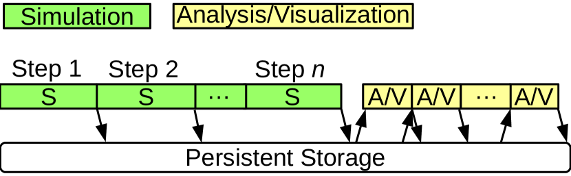
(a) Post-hoc processing

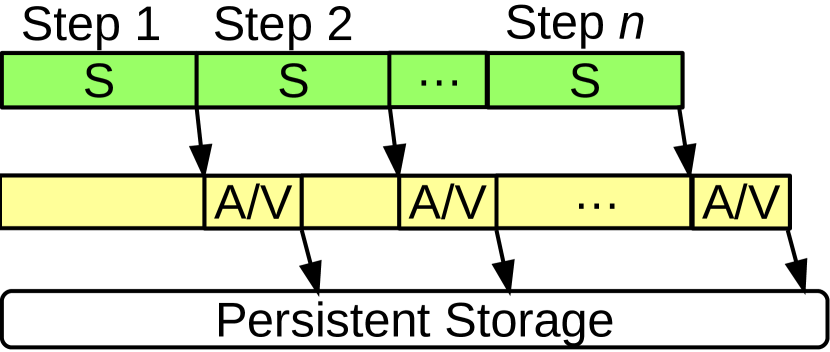
(b) In-situ workflow

Figure 1. Post hoc processing vs. in-situ workflows

In our context, a workflow is a directed acyclic graph (DAG), with application components as nodes and data as edges. Components are typically coupled by using a higher-level programming model or language, thus exposing a structure that can be exploited for performance modeling and optimization. In a file-based post-hoc processing workflow, component applications are executed in an order determined by their data dependencies. For example, in Fig. 1(a), when the simulation finishes, it saves data to persistent storage; only then can the analysis/visualization, which processes the data, be started. Performance optimization can then proceed in two steps. First, we model the performance of each component independently. Second, we find the best configuration based on the DAG and the component models.

In contrast, as shown in Fig. 1(b), component applications in an in-situ workflow run concurrently, exchanging data via network or shared memory. Workflow performance is determined by the complex interplay of the applications, which may involve factors such as load imbalances, contending network bandwidth, synchronizations, and locks (Fu et al., 2018). High performance requires that the component applications execute in a balanced and coordinated way.

For an in-situ workflow, performance optimization cannot simply be done with separate performance models of each component application due to the complicated interactions among component applications. Instead, a performance model for the whole workflow must be built, and all parameters from all components should be optimized together. For empirical model-based auto-tuners, the fact that an in-situ workflow includes multiple coupled components raises considerable challenges. Because all parameters from all components must be considered together, the potential parameter combinations increases multiplicatively. For example, in the two-component workflows of §7.1, the configuration space sizes are more than 10${}^{5}\times$ larger than those of their component applications. This dramatically raises the number of configurations to be measured as training samples for building a usable surrogate model. However, for in-situ workflows, it is not realistic to measure many parameter combinations, given the high resource consumption of running HPC applications.

Without fundamentally renovating auto-tuning algorithms, particularly the techniques used to build the surrogate model, auto-tuners for in-situ workflows face a difficult dilemma—whether to suffer a prohibitive cost in creating the accurate surrogate model needed for optimal performance, or to tolerate the poor performance associated with an inaccurate surrogate model generated at an affordable cost.

The CEAL algorithm proposed in this paper fundamentally improves the techniques to build surrogate models, such that auto-tuner cost can be reduced substantially while retaining high performance. The large resources needed to run a complete workflow repeatedly when building an auto-tuner, data collection costs are usually limited in practical settings by a resource budget. Thus, in this scenario, the advantage of the algorithm is reflected by improving the performance of the auto-tuner within a cost budget.

3. Overview of the CEAL Approach

We now introduce the methods that CEAL uses to identify well-performing configurations for in-situ workflows, by building surrogate models with limited sampling costs.

3.1. Basic Idea

As auto-tuning cost is dominated by the collection of training samples, we must select training samples carefully and use them effectively, instead of selecting training samples indiscriminately and extensively (e.g., by random sampling). The general idea of intelligent sampling has been explored in different ways in ML and in auto-tuner designs (Mametjanov et al., 2015; Behzad et al., 2019; Thiagarajan et al., 2018; Marathe et al., 2017). Our work is distinguished by how we exploit the workflow structure (§2.2) to develop special techniques that are particularly effective for auto-tuning in-situ workflows.

Our approach leverages the following two characteristics of in-situ workflows: 1) An in-situ workflow consists of multiple components, which can run independently and may be reused across workflows. 2) The interaction among components means that if any component performs poorly, the workflow is unlikely to achieve high performance.

These characteristics suggest that we should avoid collecting samples in which a workflow performs poorly, as such samples are unlikely to help with finding well-performing configurations. But how are we to avoid collecting poor-performing samples in the absence of a performance model, which is why we want those samples in the first place? We employ two ideas. 1) Leveraging the first characteristic, we build performance models for individual component applications. Because the parameter spaces of component applications are much smaller than that of the in-situ workflow, these models can be built at low cost, i.e., with only a few component application runs. (Component reuse across workflows can allow for the reuse of their models, further lowering costs.) 2) Leveraging the second characteristic, plus the component models that we have just developed, we build a simple low-fidelity model that we use to guide our search for well-performing configurations for the whole in-situ workflow, and focus sample collection on these configurations.

We also investigated other techniques that improve the selection of training samples and thus may be integrated in our solution. Active learning iteratively uses the model that is being refined to identify configurations that may lead to good performance, and focuses sample collection on those configurations (Mametjanov et al., 2015; Behzad et al., 2019). Our approach similarly focuses on well-performing configurations, as we discuss in §5. We also explored the use of configurations with much smaller inputs (i.e., much lower cost) for model building (Marathe et al., 2017). However, we found that programs often display quite different behaviors if input sizes (and problem sizes) change considerably, as when a reduced working set, corresponding to a smaller input, can fit into memory or cache. Thus, this technique cannot be used in general when auto-tuning in-situ workflows.

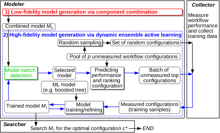
Figure 2. Structure of CEAL auto-tuning.

3.2. The CEAL Algorithm Introduced

To implement these ideas, we design the Component-based Ensemble Active Learning (CEAL) auto-tuning algorithm shown in Fig. 2. CEAL consists of two main phases.

In the Low-fidelity Model Generation via Component Combination phase, the red rectangle in Fig. 2, we build performance models for a workflow’s component applications which we combine to form a simple yet integral workflow model. This simplicity means that the integral model can be obtained at low cost but yields only approximate predictions. We use this low-fidelity workflow model ($M_{0}$ in Fig. 2) in the second phase, to evaluate configurations.

In the High-fidelity Model Generation via Dynamic Ensemble Active Learning phase, the orange dashed rectangle in Fig. 2, we use a series of samples selected based on low-fidelity model scoring to establish and improve a second, high-fidelity model of the workflow ($M_{1}$ in Fig. 2). This is the surrogate model that the searcher will use to predict workflow performance so as to find an ideal configuration.

The high-fidelity model is primitive when first established, but keeps evolving as more samples are collected and used in training, and may become a better choice for evaluating configurations than the low-fidelity model. Thus, we use a model switch detection module to monitor the two models, and switch to using the high-fidelity model to evaluate configurations when it becomes a better choice. We stop evolving the high-fidelity model when the cost budget is reached (i.e., we have tested a preset number of configurations).

We introduce these two phases in the next two sections, after which we present the detailed algorithm.

4. Generating the Low-fidelity Model

We use the low-fidelity model to evaluate configurations by predicting how well the workflow may perform. The main challenge is to build a usable model with minimal cost, such that the auto-tuner can quickly start from it and use it to build and improve the high-fidelity model.

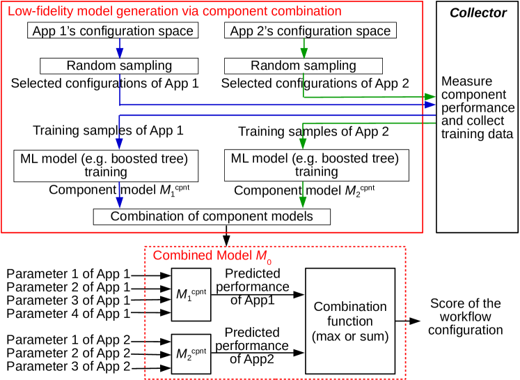
Figure 3. Combining component models.

We build the low-fidelity model by first constructing and then combining predictive models for the component applications: see Fig. 3. Each individual component model, $M_{j}$ ($j=1,2,\cdots$), outputs a performance prediction for its component for a given configuration. Its predictions should be aligned with the optimization goal of the auto-tuner; for example, execution times if the goal is shortening execution times. Component models can be built by using conventional methods, e.g., by randomly selecting configurations to collect samples and then training a boosted tree ML model. Since component applications are independent, they may be used separately or in other workflows. Costs can be reduced by including measurements collected in earlier runs in training, or by reusing models developed for other workflows. Due to space limitations, we do not elaborate here on how to build or reuse these models, but focus on how to combine component models to form the integral low-fidelity model.

There are two issues in forming the low-fidelity model. The first is what the model should output. As we will use this model only to choose among configurations, we do not need it to predict workflow performance directly. Instead, we make it output for each configuration just a score indicating how well the workflow performs relative to other configurations.

The second issue is how to combine per-component model results to build a low-fidelity model with minimal cost. One approach, which for later quantitative comparison we implement in an algorithm called ALpH, is to train a component-combining model $M_{0}$ from both component model predictions and actual workflow runs. That is, for each candidate configuration $c$, we use the $\{M_{j}\}$ to predict the performances, $\{P_{j}\}$, of the components for $c$; run the workflow with $c$, measuring its performance $p$; and add $\{c,\{P_{j}\},p\}$ to the training set for $M_{0}$. ALpH uses AL (Mametjanov et al., 2015) to select the configurations for which it generates such workflow training samples.

A deficiency of this approach is that it does not exploit any knowledge of the workflow structure. An alternative, which we use in CEAL, is to use a simple function (e.g., max, min, sum), chosen according to the performance metric being optimized by the auto-tuner, to combine the component model predictions. We select this function as follows. If the performance metric is determined largely by the bottleneck components, such as execution time and throughput, we use max (for execution time) or min (for throughput). If the performance metric is largely an aggregation of the shares from all components, such as computing resource and energy consumption, we use sum. Notice that CEAL, unlike ALpH, does not need to run the workflow. We examine the relative accuracy and costs of CEAL and ALpH below.

We postpone detailed evaluation to §7, but report here on a study in which we use two optimization objectives with different metrics—shortening execution time and minimizing computer time—to illustrate and characterize the function approach. We define execution time as wall-clock time and computer time as the number of core-hours consumed by workflow execution. We define the functions used to determine a configuration’s scores as follows.

(1) $$\emph{Score}^{\textrm{e}}(c)=\max\limits_{j}{t^{\textrm{e}}}(c_{j}),\vspace{-1ex}$$

(2) $$\emph{Score}^{\textrm{c}}(c)=\sum\limits_{j}{t^{\textrm{c}}}(c_{j}),\vspace{-1ex}$$

where for a configuration $c$, $\emph{Score}^{\textrm{e}}(c)$ and $\emph{Score}^{\textrm{c}}(c)$ are the execution and computer times (the lower, the better) of configuration $c$; $c_{j}$ is the parameter values related to component $j$ extracted from $c$; and $t^{\textrm{e}}(c_{j})$ and $t^{\textrm{c}}(c_{j})$ are the model-predicted execution and computer times of the $j^{\textrm{th}}$ component.

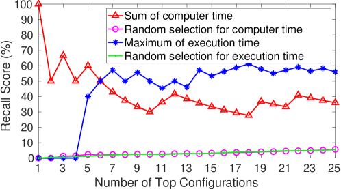
Figure 4. Recall scores based on combination functions.

To illustrate the effectiveness of this approach, Fig. 4 shows the recall scores of the low-fidelity models (Eqns 1 and 2) when used to score 500 randomly selected configurations for workflow LV. (For details on experimental settings, see §7.) Recall scores reflect the possibility that the highest-scoring configurations lead to high workflow performance (§7.2.2). To calculate recall scores, we rank configurations based both on their model-predicted scores and on the performance observed when the workflow is executed with them. The recall score of the top $n$ configurations is then the ratio between 1) the number of common configurations found in the top $n$ configurations on these ranked lists and 2) $n$. We see that the models achieve recall scores above 30% for top 5 to 25 configurations, much higher than those of random selection. This verifies that even using simple functions in the low-fidelity model can effectively locate good configurations.

The solution described in this section mainly targets loosely-coupled in-situ workflows (Fu et al., 2018; Subedi et al., 2018), in which components are coupled via high-level libraries (e.g., ADIOS (Liu et al., 2014), Flexpath (Dayal et al., 2014), DataSpaces (Docan et al., 2012), FlexIO (Zheng et al., 2013), GLEAN (Vishwanath et al., 2011), DIMES (Zhang et al., 2017), Decaf (Dreher and Peterka, 2017), or Zipper (Fu et al., 2018)). The relative ease of development and deployment of loosely-coupled in-situ workflows relative to tightly-coupled in-situ workflows makes the former much more prevalent. However, our solution can easily be adapted to optimize tightly-coupled in-situ workflows.

5. Generating the High-fidelity Model

To build the high-fidelity model, CEAL first creates a sample pool $C_{\textrm{pool}}$ by selecting configurations randomly from the workflow’s configuration space $C$. All configurations used subsequently to train the high-fidelity model are selected from $C_{\textrm{pool}}$. As we evolve the model, we repeatedly evaluate and rank all configurations remaining in $C_{\textrm{pool}}$; thus, we want $|C_{\textrm{pool}}|\ll|C|$ to keep evaluation costs manageable. However, we also want $C_{\textrm{pool}}$ to be reasonably representative of $C$ and, in particular, to contain enough well-performing configurations to train a good high-fidelity model. Say that we want the best configuration in $C_{\textrm{pool}}$ to be in the top 1/$n$ of all configurations, with probability $P$. With a pool size $p$, the chance of selecting $p$ configurations each not in the top 1/$n$ is less than $(1-1/n)^{p}$. Thus, we want $p\approx-n\cdot\ln(1-P)$, because $P>1-(1-1/n)^{p}=1-[(1-1/n)^{n}]^{p/n}>1-(1/e)^{p/n}$. For example, if 1/$n$ = 1/500 = 0.2% and $P$ = 98.2%, then $p\approx$ 2000.

To establish the high-fidelity model, CEAL selects $m_{0}$ configurations at random from $C_{\textrm{pool}}$; selects the $m_{B}$ best of the configurations remaining in $C_{\textrm{pool}}$, based on scores from the low-fidelity model; runs the workflow with the $m_{0}+m_{B}$ selected configurations; and uses the results as samples to train an initial high-fidelity model. We discuss the factors influencing the choice of $m_{B}$ and $m_{0}$ below.

To evolve the model, CEAL evaluates the configurations remaining in $C_{\textrm{pool}}$ and selects the $m_{B}$ highest-scoring. Then, it runs the workflow with those configurations and uses those results to train the high-fidelity model further. It repeats these operations until the cost budget is reached.

The high-fidelity model is initially primitive and thus the low-fidelity model is a superior choice for evaluating configurations. As more training data are acquired, the high-fidelity model eventually outperforms the low-fidelity model. Thus, we monitor the capability of the high-fidelity model in evaluating configurations, and substitute it for the low-fidelity model when it becomes a better choice. Specifically, each time that we perform more runs, we use the new data to compute the top-1, top-2, and top-3 recalls (see §7.2.2) of the low- and high-fidelity models: that is, the extent to which their best 1, 2, and 3 configurations, respectively, match the best 1, 2, and 3 as determined by experiment. When these scores for the high-fidelity model (summed to increase stability) exceed the low-fidelity sum, we switch to the high-fidelity model.

As we show quantitatively when we present experimental results in §7, the power of the CEAL approach derives from the fact that it selects mostly top configurations when collecting data to train the high-fidelity model. The rationale here is this: our ultimate goal is a surrogate model that the searcher can use to find the best configurations, and for that purpose it should be highly accurate for good configurations, but can be less accurate for bad configurations. Thus, we prefer to use our limited sample budget for samples collected for high-performing configurations. (Focusing sample collection on high-performing configurations also has the useful side effect that these samples, by definition, take less time.)

Thus, as described above, we use the low-fidelity model to bootstrap the sample selection process, and transition to the high-fidelity trained model as the number of samples grows. But what if our low-fidelity model is biased in such a way that it never gives good scores to high-performing configurations? Then the high-fidelity model may never improve. This concern motivates us to select, in the first phase, $m_{0}$ random configurations as well as the $m_{B}$ configurations selected with the low-fidelity model. We discuss the sensitivity of CEAL to these hyper-parameters in §7.6.

6. CEAL Algorithm

The CEAL algorithm, Alg. 1, takes as input a data collection budget ($m$), expressed in terms of workflow runs for simplicity. (If a budget on real resource consumption is preferred, the algorithm can be adapted to monitor the resource consumption of the workflow and its component applications.)

Lines 1–7, the low-fidelity model generation via component combination phase, run each component application $m_{\textrm{R}}$ times to test randomly selected configurations and build component models. The cost is equivalent to running the complete workflow $m_{\textrm{R}}$ times, incurring a charge of $m_{\textrm{R}}$ from budget $m$ (Line 9). If a component application has been tested earlier in other workflows, some configuration-performance data $D_{j}^{\textrm{hist}}$ can be reused to further improve component model quality (Line 4). In the case, $m_{\textrm{R}}$ should be close to 0. Otherwise, $m_{\textrm{R}}$ is generally set to be from $m\cdot 20\%$ to $m\cdot 70\%$.

Algorithm 1 Component-based Ensemble Active Learning
Inputs: Workflow runs budget $\bm{m}$; budget used to run component applications $\bm{m_{\textbf{{R}}}}$; for each component application $1\leq j\leq J$, configuration space $\bm{C}_{j}$ and historical measured configuration-performance samples $\bm{D}_{j}^{\textbf{{hist}}}$; sample pool $\bm{C}_{\textbf{{pool}}}$; number of initial random samples $\bm{m_{0}}$; number of iterations $\bm{I}$.
Output: High-fidelity workflow model $\bm{M_{\textrm{H}}}$.

1:for $j\in\{1,2,\cdots,J\}$ do

2:    Randomly select $m_{\textrm{R}}$ configurations from $C_{j}$ as $C_{j}^{\textrm{meas}}$;

3:    Run $j$^th component with configurations in $C_{j}^{\textrm{meas}}$, giving $D_{j}^{\textrm{meas}}$;

4:    $D_{j}^{\textrm{meas}}\leftarrow D_{j}^{\textrm{meas}}\cup D_{j}^{\textrm{hist}}$;

5:    Train component model $M_{j}^{\textrm{cpnt}}$ with $D_{j}^{\textrm{meas}}$ for the $j$^th application;

6:end for

7:Generate low-fidelity model $M_{\textrm{L}}$ from component models and combination function (see §4);

8:Move $m_{0}$ randomly selected configurations from $C_{\textrm{pool}}$ to form $C_{\textrm{meas}}$;

9:$m_{B}\leftarrow(m-m_{0}-m_{\textrm{R}})/I$;

10:Score all configurations in $C_{\textrm{pool}}$ with $M_{\textrm{L}}$;

11:Move top $m_{B}$ configurations from $C_{\textrm{pool}}$ into $C_{\textrm{meas}}$;

12:$M\leftarrow M_{\textrm{L}}$;     // Set the model used for evaluating configurations

13:$M_{\textrm{H}}\leftarrow$ ML model (e.g., boosted tree (Chen and Guestrin, 2016)); // Init high-fidelity model

14:for $i\in\{1,\cdots,I\}$ do

15:    Run workflow for all configurations in $C_{\textrm{meas}}$, giving $D_{\textrm{meas}}$;

16:    if $M=M_{\textrm{L}}$ then    // Begin model switch detection

17:        // Score models: recalls for top 1, 2, 3 configurations

18:        $S_{\textrm{H}}=\sum_{i=1,2,3}S_{r}(i,C_{\textrm{meas}},M_{H},D_{\textrm{meas}})$;   // See §7.2.2

19:        $S_{\textrm{L}}=\sum_{i=1,2,3}S_{r}(i,C_{\textrm{meas}},M_{L},D_{\textrm{meas}})$;    // See §7.2.2

20:        if $S_{\textrm{H}}\geq S_{\textrm{L}}\ \textbf{then}\ M\leftarrow M_{\textrm{H}}$ endif;

21:    end if     // End model switch detection

22:    Use $D_{\textrm{meas}}$ to train/refine $M_{\textrm{H}}$, and update $M$ if it switched to $M_{\textrm{H}}$;

23:    Use $M$ to evaluate the configurations in $C_{\textrm{pool}}$;

24:    Move the top $m_{B}$ configurations from $C_{\textrm{pool}}$ to form $C_{\textrm{meas}}$ again;

25:end for

26:return $M_{\textrm{H}}$.

The second phase, high-fidelity model generation via dynamic ensemble active learning, is Lines 8–26. First, $m_{0}$ random training samples are selected (Line 8) to characterize the overall performance distribution of the workflow over all configurations. In general, $m_{0}$ is set to be from $m\cdot 5\%$ to $m\cdot 45\%$, depending on workflow structure and optimization objective. Sensitivity studies reported in §7.6 show that CEAL is insensitive to the values used for $m_{\textrm{R}}$ and $m_{0}$ in a large range. We recommend $m_{0}\approx 25\%\cdot m$ when $|D_{j}^{\textrm{hist}}|\gg m$ ($j$=1,…,$J$) and thus $m_{\textrm{R}}$=0, and $m_{0}\approx 15\%\cdot m$ if no historical measurements are available (i.e., $|D_{j}^{\textrm{hist}}|$=0). Then, top configurations are selected (Lines 11, 24) based on the evaluation with model $M$. (Lines 16–21 handle the switching from low-fidelity to high-fidelity model.) The high-fidelity model is retrained repeatedly as more training data are acquired (Lines 14–25), and returned as the output of the algorithm.

7. Experimental Evaluation

We describe our benchmarks (§7.1), evaluation metrics (§7.2), and comparison targets (§7.3). Then, we evaluate the performance of CEAL and other algorithms in a general auto-tuning scenario without historical measurements, and investigate reasons for CEAL’s superiority (§7.4). We also consider optimization with historical component measurements, and compare CEAL with an algorithm that incorporates component performance by training a ML model (§7.5). Finally, we study CEAL’s sensitivity to hyper-parameter values (§7.6).

7.1. Experimental Setup

We conducted experiments on a 600-node cluster with Intel Omni-Path Fabric Interconnect. Each node has two 18-core 2.10GHz Intel Broadwell Xeon E5-2695 v4 processors with hyperthreading disabled and 128 GB DDR4 SDRAM. We ran each workflow with exclusive access to node resources, on allocation sizes up to 32 compute nodes. We used three in-situ workflows, namely LV, HS, and GP, in our experiments:

LV couples two components: the LAMMPS (LAMMPS Molecular Dynamics Simulator, 2019) molecular dynamics simulator and Voro++ (Voro++, 2019), a Voronoi tesselator. LV involves full-featured, realistic applications coupled via ADIOS. The sample run used here simulates $16\,000$ atoms and streams position and velocity data into the tesselator for analysis and visualization. This application is a model for many cases in particle simulation and visualization.

HS also couples two components: a Heat Transfer (Heat Transfer, 2019) simulation with an analysis application, Stage Write. Heat Transfer is a mini-application that runs the heat equation over the grid of a given size and forwards simulation state over ADIOS to Stage Write, which produces output in the file system. This application is a model for many cases in numerical PDE calculations and I/O buffering and forwarding.

GP couples four components: Gray-Scott reaction-diffusion simulation; an analysis application, PDF calculator, applied to the Gray-Scott output; a visualization application, G-Plot, also applied to Gray-Scott output; and a second visualization application, P-Plot, applied to PDF output. GP involves applications of intermediate complexity, also coupled via ADIOS. Two component applications, Gray-Scott and PDF calculator are configurable, but G-Plot and P-Plot are not. This application is a model for many cases in chemical reaction dynamics and more complex multi-purpose analysis workflows.

Table 1. Parameter spaces for our three target workflows

Workflow	Application	Parameter	Options
		# processes	2, 3, $\cdots$, $1085$
	LAMMPS	# processes per node	1, 2, $\cdots$, 35
LV		# threads per process	1, 2, 3, 4
		# steps in an IO interval	50, 100, $\cdots$, 400
		# processes	2, 3, $\cdots$, $1085$
	Voro++	# processes per node	1, 2, $\cdots$, 35
		# threads per process	1, 2, 3, 4
		# processes in X	2, 3, $\cdots$, 32
	Heat	# processes in Y	2, 3, $\cdots$, 32
HS	transfer	# processes per node	1, 2, $\cdots$, 35
		# IO writes	4, 8, $\cdots$, 32
		buffer size (MB)	1, 2, $\cdots$, 40
	Stage	# processes	2, 3, $\cdots$, $1085$
	write	# processes per node	1, 2, $\cdots$, 35
	Gray-	# processes	2, 3, $\cdots$, 1085
GP	Scott	# processes per node	1, 2, $\cdots$, 35
	PDF	# processes	1, 2, $\cdots$, 512
	calculate	# processes per node	1, 2, $\cdots$, 35
	Gray plot	# processes	1
	PDF plot	# processes	1

Application configuration options, shown in Tbl. 1, form a total of 2.3 $\times$ 10¹⁰ possible configurations for LV (LAMMPS: 6.1 $\times$ 10⁵; Voro++: 7.6 $\times$ 10⁴), 5.1 $\times$ 10¹⁰ for HS (Heat Transfer: 5.4 $\times$ 10⁶; Stage Write: 1.9 $\times$ 10⁴), and 8.5 $\times$ 10⁷ for GP (Gray-Scott: 1.9 $\times$ 10⁴; PDF calculator: 9.0 $\times$ 10³). We obtained expert-recommended configurations for each.

In order to compare expert-recommended vs. good configurations, we generated for each workflow, as $C_{\textrm{pool}}$, 2000 configurations of randomly selected parameter values. Then, for each such configuration, we launched all workflow components at once and recorded each component’s end-to-end wall-clock time. We then used the longest component execution time as the configuration’s execution time, and the product of execution time, number of computing nodes used, and number of cores per node as the configuration’s computer time. We list in Tbl. 2 the expert-recommended and best configurations for each workflow and optimization objective, and their achieved performance. The expert recommendations only do well for GP. (Since the unconfigurable G-Plot is the bottleneck in GP, many GP configurations have similar execution times, close to that of G-Plot alone, 97.0 seconds.)

Table 2. Configurations and performance of benchmarks

Wf.	Objective	Option	Performance	Configuration
	Exec. time	Best	27.2 secs	(430, 23, 1, 300, 88, 10, 4)
LV		Expert	36.8 secs	(288, 18, 2, 400, 288, 18, 2)
	Comp. time	Best	3.36 core-hrs	(175, 35, 2, 400, 38, 29, 3)
		Expert	4.15 core-hrs	(18, 18, 2, 400, 18, 18, 2)
	Exec. time	Best	6.02 secs	(13, 17, 14, 4, 29, 19, 3)
HS		Expert	28.0 secs	(32, 17, 34, 4, 20, 560, 35)
	Comp. time	Best	0.517 core-hrs	(5, 25, 35, 4, 3, 5, 3)
		Expert	0.894 core-hrs	(8, 4, 32, 4, 20, 35, 35)
	Exec. time	Best	98.7 secs	(175, 13, 24, 23, 1, 1, 1)
GP		Expert	102 secs	(525, 35, 525, 35, 1, 1)
	Comp. time	Best	6.95 core-hrs	(66, 34, 41, 22, 1, 1)
		Expert	5.85 core-hrs	(35, 35, 35, 35, 1, 1)

We also measured the execution and computer times of 500 configurations randomly selected from the parameter space of each configurable component application, and used these samples as component measurements, from which CEAL may select training samples for component models.

7.2. Evaluation Metrics

We use three metrics to evaluate auto-tuning algorithms.

7.2.1. Performance of Best Predicted Configuration

As our goal is to optimize the execution time and computer time of in-situ workflows, the execution and computer time achieved by the best configuration predicted for a workflow is an important evaluation metric.

7.2.2. Robustness in Finding Top Configurations

We use the recall score to measure the error tolerance of an autotuning algorithm in predicting top configurations. As defined by Marathe et al. (Marathe et al., 2017), recall score is, for a value $n$, the percentage of configurations as predicted by the algorithm that are actually within the top $n$ configurations. Given a set of configurations c for which we have workflow performance data $\textbf{D}_{\textbf{c}}$, a model M for scoring configurations, and a function top$(n,s)$ for selecting the top $n$ entries from a set of scored configurations $s$, the recall score for $n$ is:

(3) $$S_{r}(n,\textbf{c},\textbf{M},\textbf{D}_{\textbf{c}})=|\textrm{top}(n,\textbf{M}(\textbf{c}))\cap\textrm{top}(n,\textbf{D}_{\textbf{c}})|/n\times 100\%.$$

A higher recall score indicates a more robust auto-tuning algorithm; in general, $S_{r}(i)$ is more important than $S_{r}(j)$ ($i<j$). For $n=1$, the recall score also represents the probability of finding the best-performing configuration.

7.2.3. Practicality in Performance Optimization

Since the data collection cost is considerable and unignorable for empirical auto-tuning algorithms, we monitor the least number of workflow runs required to pay off the auto-tuning cost, and use that metric to evaluate the practicality of auto-tuning algorithms. The least number of uses is $N=c/\Delta p$. Here, $\Delta p$ is the actual improvement per workflow execution in the optimization objective (execution time or computer time reduction) achieved by the auto-tuning algorithm relative to an expert recommendation, and $c$ is the training data collection cost incurred in achieving the performance optimization objective, i.e., the sum of the workflow’s execution times or computer times over all training samples.

7.3. Comparison Targets

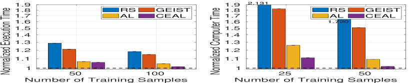
(a) LV

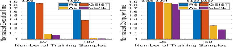
(b) HS

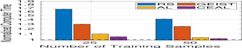
(c) GP

Figure 5. The best configuration auto-tuned w/o historical measurements (dashed lines: the best configuration in the test set)

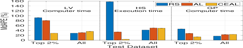
Figure 6. Prediction accuracy of models in autotuning w/o historical measurements

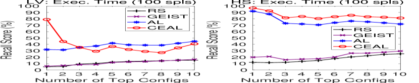
(a) Optimizing execution time of LV and HS

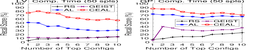
(b) Optimizing computer time of LV and GP

Figure 7. Robustness of autotuning w/o historical measurements

Since there exist few auto-tuning algorithms customized for in-situ workflows, we compare CEAL with three auto-tuning algorithms for general HPC applications. RS selects training data by random sampling. AL is a typical AL algorithm that iteratively selects a batch of the best configurations predicted by gradually refined models as training samples (Mametjanov et al., 2015; Behzad et al., 2019). GEIST, a state-of-the-art AL-based auto-tuning algorithm for finding performance-optimizing configurations (Thiagarajan et al., 2018) is guided by a parameter graph to choose training samples with the highest possibility of being optimal (defined as in top 5% configurations) in each iteration. We also report in §7.5.2 on comparisons with a variant of CEAL, ALpH (introduced in §4) that uses learning to combine component models.

In all algorithms, we use the xgboost.XGBRegressor implementation of extreme gradient boosting regression as the original ML model. We adjust GEIST, AL, ALpH, and CEAL hyperparameters with and without historical measurements, and $I$, $m_{0}$, and $m_{\textrm{R}}$ in CEAL, and select the best settings for each algorithm. Hyperparameter optimization methods (Xia et al., 2017) are beyond the scope of this paper. In all experiments, we run each algorithm 100 times and report averages.

7.4. Autotuning without Historical Measurements

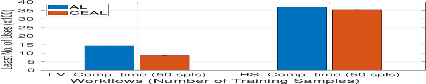
Figure 8. Practicality of autotuning w/o historical measurements

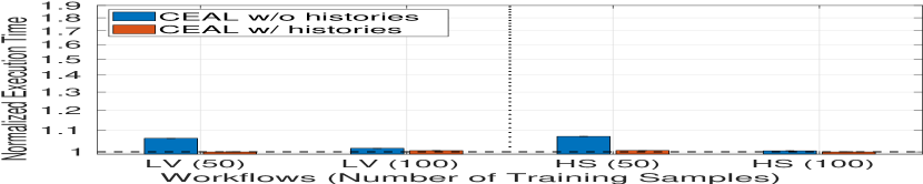
(a) Execution time of predicted best conf.

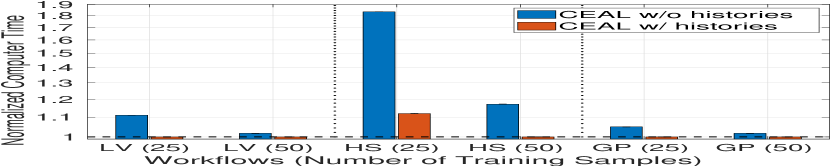
(b) Computer time of predicted best conf.

Figure 9. Effect of historical measurements on CEAL (dashed lines: best test config.)

We first examine the overall performance of our auto-tuner in the absence of historical measurements. We compare the actual performance of workflows auto-tuned by CEAL and others (§7.4.1), and explain CEAL’s superiority by experimentally validating its design principle (§7.4.2). Also, we investigate CEAL’s robustness and practicality (§7.4.3 and §7.4.4). (When comparing costs, we consider the cost of running an in-situ workflow as being comparable to the total cost of running all of its component applications separately.)

7.4.1. Actual Performance of Auto-tuned Workflows

We measured the actual execution and computer time of the best configurations of LV, HS, and GP predicted by RS, GEIST, AL, and CEAL, and plot normalized values in Fig. 5, with the performance of the best configuration in the test set shown as “1” (the same for Figs. 9 and 12). We test CEAL with different numbers $m$ of training samples by doubling $m$ from 25 until the auto-tuned performance of LV is at most 5% worse than the best. We show here results for the largest two values of $m$ tested: 100 and 50 for execution time and 50 and 25 for computer time. For consistency, we also select the same $m$ for all workflows in all experiments. Fig. 5 shows that the execution and computer times achieved by CEAL are always better than by RS, GEIST, and AL. For example, CEAL improves both execution and computer time by 14–72% relative to RS and 12–60% relative to GEIST—and LV computer time relative to LV by 11.9% and 6.9% with 25 and 50 training samples, respectively. CEAL outperforms AL, because performance models trained with the same number of training samples are much more accurate for component applications than in-situ workflows, and our method of determining workflow performance provides relatively accurate configuration ranking over top configurations.

7.4.2. Why CEAL Outperforms RS and AL

The absolute percentage error (APE) of a sample $i$ is $|(y_{i}-y^{\prime}_{i})/y_{i}|$, where $y_{i}$ is actual performance and $y^{\prime}_{i}$ is predicted performance. The median APE (MdAPE) for a set of samples is a commonly used measure of model prediction quality. To further understand why CEAL beats AL and RS, we plot in Fig. 7 the MdAPEs of models generated by RS, AL, and CEAL when used to predict performance over all, and the top 2%, of test dataset configurations. CEAL MdAPEs are much less than those of RS and AL for the top 2% of configurations; as a result, CEAL outperforms RS and AL, even though its MdAPEs are comparable to, or a little higher than, those of RS and AL over all configurations. This result verifies our intuition that picking higher-performance configurations can improve prediction accuracy for top configurations, and thus make best use of the few training samples allotted.

7.4.3. Robustness of Auto-tuning Algorithms

We use the recall scores (§7.2.2) of the top $n$ ($n=1,\cdots,10$) configurations to evaluate the robustness of RS, GEIST, AL, and CEAL in auto-tuning our workflows for execution time and computer time. We see in Fig. 7 that CEAL is more robust than RS, GEIST, and AL in most cases. For the top-one configuration recall score (the most important performance measure), CEAL achieves 76% (or 79%) when optimizing the computer (or execution) time of LV with 50 training samples, as against 4% (or 5%), 12% (or 6%), and 51% (or 32%) for RS, GEIST, and AL. For instance, although CEAL’s recall score is lower than that of AL for the top 4 to 10 configurations for LV, it still obtains a better execution time.

7.4.4. Practicality of Auto-tuning Algorithms

We examine the practicality of the four auto-tuning algorithms in optimizing the computer time of LV and HS. Since the computer time of LV/HS achieved by RS and GEIST with only 25 and 50 training samples is worse than that at the expert-recommended configuration, the practicality of RS and GEIST is limited. Then, we focus on auto-tuning the computer time of LV and HS by AL and CEAL with 50 training samples, and plot the least number of runs (§7.2.3) in Fig. 9, which reveals that CEAL is superior to AL in terms of practicality. In particular, LV is worth auto-tuning by CEAL if it is expected to run 864 times, 40% less than the 1444 times required for AL. We attribute CEAL’s superiority to its more accurate selection of training samples that take less computer time, as boosted by the combined low-fidelity model.

7.5. With Historical Component Measurements

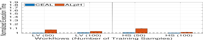
(a) Optimizing execution time

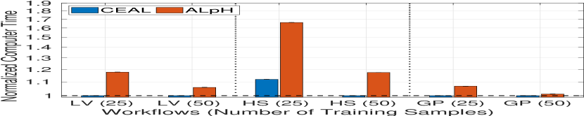
(b) Optimizing computer time

Figure 10. Best configuration auto-tuned with histories (dashed lines: best test config.)

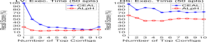
(c) Optimizing execution time of LV and HS

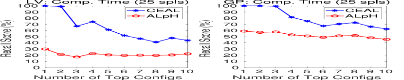
(d) Optimizing computer time of LV and GP

Figure 11. Robustness of autotuning with historical measurements

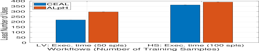
(a) Optimizing execution time

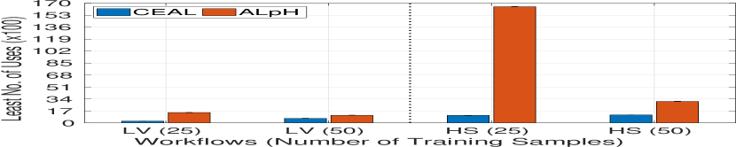
(b) Optimizing computer time

Figure 12. Practicality of autotuning with historical measurements

Since component historical measurements are often available, we next examine auto-tuner performance when historical measurements are considered. We show that CEAL can make good use of component measurements to enhance workflow performance (§7.5.1) and auto-tuner practicality (§7.5.4). We also demonstrate the superiority of CEAL over ALpH’s component integration method (§7.5.2, §7.5.3).

7.5.1. Effect of Previous Component Measurements

If historical performance measurements are available for component applications, then CEAL can use those measurements to train component application models without charge against its training sample budget, and then perform more full workflow runs that would otherwise be possible. In order to explore the benefits that result, we compare workflow performance when optimized by CEAL with and without historical measurements. In the first case, we assume no historical measurements, and thus subtract the $m_{R}$ component samples used to train component models from CEAL’s training sample budget; in the second, we treat those measurements as historical and do not count them toward the cost. We see from Fig. 9 that historical measurements improve CEAL performance in all cases. In addition, Fig. 9(b) shows that historical measurements help CEAL, in the case of 25 training samples, reduce computer time for LV by 10.0%, HS by 38.9%, and GP by 4.8%. We conclude that CEAL can make effective use of historical component measurements.

7.5.2. Actual Performance of Auto-tuned Workflows

Recall from §4 that ALpH differs from CEAL in using learning rather than functions to combine component model performance predictions. To compare these approaches to combining component models, we measure LV, HS, and GP performance when auto-tuned by ALpH and CEAL with different numbers of training samples. The normalized execution and computer times in Fig. 12 show that CEAL is superior to ALpH in all cases. For example, we see in Fig. 10(b) that the computer times of LV, HS, and GP when optimized by CEAL with 25 training samples are 15.1%, 32.6%, and 6.5% less than when optimized by ALpH, respectively. We attribute CEAL’s outperforming ALpH with the same historical measurements to CEAL’s component combination using training samples more efficiently than ALpH’s model-based approach.

7.5.3. Robustness of Auto-tuning Algorithms

We also evaluate the robustness of ALpH and CEAL with historical component measurements in optimizing the execution and computer time of our in-situ workflows. The recall scores (§7.2.2) at top configurations are plotted in Fig. 12; we see that CEAL is always more robust than ALpH. CEAL’s best-1 and best-2 configuration recall scores are both above 99%.

7.5.4. Practicality of Auto-tuning Algorithms

We examine the practicality of ALpH and CEAL with historical component measurements for auto-tuning LV and HS, and plot the number of runs (§7.2.3) in Fig. 12. It can be observed that when CEAL is used to optimize LV execution time with 50 training samples and LV computer time with 25 training samples, the number of LV runs (§7.2.3) required to recoup the auto-tuning cost is only 219 and 269, implying great practicality of CEAL. As to the execution time cost, we consider workflow instances at training configurations to run sequentially, even though the training data collection can sometimes be completed in parallel.

7.6. Hyper-parameter Sensitivity Analysis

We use LV, when predicting the best computer time with 50 training samples, to study CEAL’s sensitivity to hyper-parameter values. Fig. 13 shows the actual computer times of the best configurations predicted in various settings. (1) We run CEAL with from 1 to 10 iterations ($I$). We see in Fig. 13(a) that LV computer time converges to the best after three iterations. (2) We test CEAL as the number of coupled random samples replaced by component samples ($m_{\textrm{R}}$) is varied from $5\%\cdot m$ to $(m-m_{0})$ at an interval of $5\%\cdot m$. Fig. 13(b) shows that LV computer time is stable over a large range of $m_{\textrm{R}}$: from 20% to 65% training samples. (3) We run CEAL as we increase the number of random samples ($m_{0}$) from $5\%\cdot m$ to $(m-m_{\textrm{R}})$ at an interval of $5\%\cdot m$. Fig. 13(c) shows that LV computer time is stable over a large range of $m_{0}$: from $5\%\cdot m$ to $35\%\cdot m$ for CEAL with historical measurements and from $5\%\cdot m$ to $75\%\cdot m$ for CEAL without historical measurements.

We have also performed these studies for our other workflows and optimization metrics, and see similar results, except that in one case we found that an $m_{0}$ value of around $45\%\cdot m$ was best, indicating that (as discussed in §5), the low-fidelity model was not performing well.

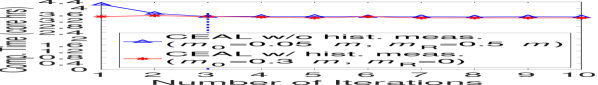
(a) $I$

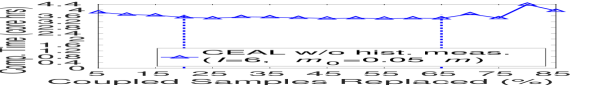
(b) $m_{\textrm{R}}$/$m$

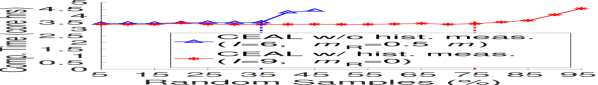
(c) $m_{0}$/$m$

Figure 13. Impact of parameter settings.

8. Related Work

Sourouri et al. (Sourouri et al., 2017) integrate fine-grained auto-tuning with user-controllable hardware switches and threads in order to use dynamic voltage and frequency scaling to improve the energy efficiency of a memory-bound HPC application. However, their application-specific analytical performance model is not directly applicable to other applications.

Popov et al. (Popov et al., 2019) reduce data collection costs by extracting and running short representative codelets, rather than whole applications, to jointly optimize page and thread mappings for applications in NUMA systems. However, this approach will not pick the optimal configuration for a whole application when that configuration is not the best of any codelet.

Some auto-tuners target storage systems. Cao et al. (Cao et al., 2018) apply and analytically compare multiple black-box optimization techiques focusing on storage systems. Li et al. (Li et al., 2017) used reinforcement learning to develop a model-less unsupervised storage parameter tuning system, CAPES. However, these studies do not take data collection costs into account.

Others have applied active learning to HPC auto-tuning (Ogilvie et al., 2017; Duplyakin et al., 2016; Balaprakash et al., 2013). GEIST uses semi-supervised learning based on a parameter graph for fast parameter space exploration (Thiagarajan et al., 2018); it can auto-tune HPC applications with configuration parameter spaces in the range of 18000. Our work targets optimizing complex HPC applications with configuration space size of 10¹⁰ or more at an affordable data collection cost.

Marathe et al. (Marathe et al., 2017) proposed an HPC application auto-tuning algorithm that used three fully connected neural networks to capture the relationship between configuration parameters and performance metrics from many cheap and a few expensive training computations. However, the small, cheap samples often have low similarity to the large, expensive samples, failing to provide transferable knowledge.

9. Conclusion

The use of machine learning (ML)-based auto-tuners has been considered infeasible for in-situ workflows due to their large configuration spaces. Our new approach achieves high-quality ML auto-tuners for in-situ workflows, even with a tight cost budget, by leveraging the fact that in-situ workflows often link multiple component applications in relatively simple structures. Specifically, our CEAL algorithm 1) combines models for component applications into a low-fidelity workflow model, and then 2) uses the low-fidelity model to guide the collection of samples for training a high-fidelity model. Experiments with three scientific in-situ workflows confirm the viability of the CEAL approach, showing it can build a high-quality auto-tuner that is better at finding best-performing configurations than auto-tuners built with other methods. In one example, CEAL with just 50 training samples optimizes workflow execution time so well than only 219 subsequent runs are required to recoup cost.

References

- (1)
- Ayachit et al. (2016) Utkarsh Ayachit, Andrew Bauer, Earl P. N. Duque, Greg Eisenhauer, Nicola Ferrier, Junmin Gu, Kenneth E. Jansenk, Burlen Loring, Zarija Lukic, Suresh Menon, Dmitriy Morozov, Patrick O’Leary, Reetesh Ranjan, Michel Rasquin, Christopher P. Stone, Venkat Vishwanath, Gunther H. Weber, Brad Whitlock, Matthew Wolf, K. John Wu, and E. Wes Bethel. 2016. Performance analysis, design considerations, and applications of extreme-scale in situ infrastructures. In IEEE/ACM SC.
- Balaprakash et al. (2018) Prasanna Balaprakash, Jack Dongarra, Todd Gamblin, Mary Hall, Jeffrey K. Hollingsworth, Boyana Norris, and Richard Vuduc. 2018. Autotuning in high-performance computing applications. Proc. of the IEEE 106, 11 (2018), 2068–2083.
- Balaprakash et al. (2013) Prasanna Balaprakash, Robert B. Gramacy, and Stefan M. Wild. 2013. Active-learning-based surrogate models for empirical performance tuning. In IEEE Cluster.
- Behzad et al. (2019) Babak Behzad, Surendra Byna, Prabhat, and Marc Snir. 2019. Optimizing I/O Performance of HPC Applications with Autotuning. ACM Transactions on Parallel Computing 5, 4 (2019), 15:1–15:27.
- Cao et al. (2018) Zhen Cao, Vasily Tarasov, Sachin Tiwari, and Erez Zadok. 2018. Towards better understanding of black-box auto-tuning: A comparative analysis for storage systems. In USENIX Annual Tech Conf. 893–907.
- Chen and Guestrin (2016) Tianqi Chen and Carlos Guestrin. 2016. XGBoost: A Scalable Tree Boosting System. In ACM SIGKDD. 785–794.
- Dayal et al. (2014) Jai Dayal, Drew Bratcher, Greg Eisenhauer, Karsten Schwan, Matthew Wolf, Xuechen Zhang, Hasan Abbasi, Scott Klasky, and Norbert Podhorszki. 2014. Flexpath: Type-based publish/subscribe system for large-scale science analytics. In CCGrid. 246–255.
- Ding et al. (2015) Yufei Ding, Jason Ansel, Kalyan Veeramachaneni, Xipeng Shen, Una-May O’Reilly, and Saman Amarasinghe. 2015. Autotuning algorithmic choice for input sensitivity. In ACM SIGPLAN PLDI. 379–390.
- Docan et al. (2012) Ciprian Docan, Manish Parashar, and Scott Klasky. 2012. DataSpaces: An Interaction and Coordination Framework for Coupled Simulation Workflows. Cluster Computing 15, 2 (2012), 163–181.
- Dreher and Peterka (2017) Matthieu Dreher and Tom Peterka. 2017. Decaf: Decoupled dataflows for in situ high-performance workflows. Technical Report ANL/MCS-TM-371. Argonne National Laboratory.
- Duplyakin et al. (2016) Dmitry Duplyakin, Jed Brown, and Robert Ricci. 2016. Active learning in performance analysis. In IEEE Cluster. Taipei, Taiwan, 182–191.
- Foster et al. (2017) Ian Foster, Mark Ainsworth, Bryce Allen, Julie Bessac, Franck Cappello, Jong Youl Choi, Emil Constantinescu, Philip E Davis, Sheng Di, Wendy Di, Hanqi Guo, Scott Klasky, Kerstin Kleese Van Dam, Tahsin Kurc, Abid Malik, Kshitij Mehta, Klaus Mueller, Todd Munson, George Ostouchov, Manish Parashar, Tom Peterka, Line Pouchard, Dingwen Tao, Ozan Tugluk, Stefan Wild, Matthew Wolf, Justin Wozniak, Wei Xu, and Shinjae Yoo. 2017. Computing just what you need: Online data analysis and reduction at extreme scales. In European Conference on Parallel Processing. Springer, 3–19.
- Fu et al. (2018) Yuankun Fu, Feng Li, Fengguang Song, and Zizhong Chen. 2018. Performance analysis and optimization of in-situ integration of simulation with data analysis: Zipping applications up. In ACM HPDC. 192–205.
- Golovin et al. (2017) Daniel Golovin, Benjamin Solnik, Subhodeep Moitra, Greg Kochanski, John Karro, and D. Sculley. 2017. Google Vizier: A service for black-box optimization. In ACM SIGKDD. 1487–1496.
- Heat Transfer (2019) Heat Transfer. 2019. https://github.com/CODARcode/Example-Heat_Transfer/blob/master/README.adoc.
- LAMMPS Molecular Dynamics Simulator (2019) LAMMPS Molecular Dynamics Simulator. 2019. https://lammps.sandia.gov.
- Li et al. (2017) Yan Li, Kenneth Chang, Oceane Bel, Ethan L. Miller, and Darrell D. E. Long. 2017. CAPES: Unsupervised storage performance tuning using neural network-based deep reinforcement learning. In IEEE/ACM SC.
- Liu et al. (2014) Qing Liu, Jeremy Logan, Yuan Tian, Hasan Abbasi and· Norbert Podhorszki, Jong Youl Choi, Scott Klasky, Roselyne Tchoua and· Jay Lofstead, Ron Oldfield, Manish Parashar, Nagiza Samatova and· Karsten Schwan, Arie Shoshani, Matthew Wolf, Kesheng Wu, and Weikuan Yu. 2014. Hello ADIOS: the challenges and lessons of developing leadership class I/O frameworks. Conc Comp: Pract Exp 26, 7 (2014), 1453–1473.
- Mametjanov et al. (2015) Azamat Mametjanov, Prasanna Balaprakash, Chekuri Choudary, Paul D. Hovland, Stefan M. Wild, and Gerald Sabin. 2015. Autotuning FPGA design parameters for performance and power. In IEEE Intl Symp on Field-Programmable Custom Computing Machines. 84–91.
- Marathe et al. (2017) Aniruddha Marathe, Rushil Anirudh, Nikhil Jain, Abhinav Bhatele, Jayaraman Thiagarajan, Bhavya Kailkhura, Jae-Seung Yeom, Barry Rountree, and Todd Gamblin. 2017. Performance modeling under resource constraints using deep transfer learning. In IEEE/ACM SC.
- Meng et al. (2019) Ke Meng, Jiajia Li, Guangming Tan, and Ninghui Sun. 2019. A pattern based algorithmic autotuner for graph processing on GPUs. In ACM PPoPP. 201–213.
- Ogilvie et al. (2017) William F. Ogilvie, Pavlos Petoumenos, Zheng Wang, and Hugh Leather. 2017. Minimizing the cost of iterative compilation with active learning. In IEEE/ACM Intl Symp on Code Gen. and Opt. 245–256.
- Popov et al. (2019) Mihail Popov, Alexandra Jimborean, and David Black-Schaffer. 2019. Efficient thread/page/parallelism autotuning for NUMA systems. In ACM ICS. 342–353.
- Sourouri et al. (2017) Mohammed Sourouri, Espen Birger Raknes, Nico Reissmann, Johannes Langguth, Daniel Hackenberg, Robert Schöne, and Per Gunnar Kjeldsberg. 2017. Towards fine-grained dynamic tuning of HPC applications on modern multi-core architectures. In IEEE/ACM SC.
- Subedi et al. (2018) Pradeep Subedi, Philip Davis, Shaohua Duan, Scott Klasky, Hemanth Kolla, and Manish Parashar. 2018. Stacker: An autonomic data movement engine for extreme-scale data staging-based in-situ workflows. In IEEE/ACM SC.
- Thiagarajan et al. (2018) Jayaraman J. Thiagarajan, Nikhil Jain, Rushil Anirudh, Alfredo Gimenez, Rahul Sridhar, Aniruddha Marathe, Tao Wang, Murali Emani, Abhinav Bhatele, and Todd Gamblin. 2018. Bootstrapping parameter space exploration for fast tuning. In ACM ICS. 385–395.
- Tillet and Cox (2017) Philippe Tillet and David Cox. 2017. Input-aware auto-tuning of compute-bound HPC kernels. In IEEE/ACM SC.
- Vishwanath et al. (2011) Venkatram Vishwanath, Mark Hereld, Vitali Morozov, and Michael E. Papka. 2011. Topology-aware data movement and staging for I/O acceleration on Blue Gene/P supercomputing systems. In IEEE/ACM SC.
- Voro++ (2019) Voro++. 2019. http://math.lbl.gov/voro++.
- Xia et al. (2017) Yufei Xia, Chuanzhe Liu, Yuying, and Nana Liu. 2017. A Boosted Decision Tree Approach using Bayesian Hyper-parameter Optimization for Credit Scoring. Expert Systems with Applications 75 (2017), 225–241.
- Yu et al. (2018) Zhibin Yu, Zhendong Bei, and Xuehai Qian. 2018. Datasize-aware high dimensional configurations auto-tuning of in-memory cluster computing. In ACM ASPLOS. 564–577.
- Zhang et al. (2017) Fan Zhang, Tong Jin, Qian Sun, Melissa Romanus, Hoang Bui, Scott Klasky, and Manish Parashar. 2017. In-memory staging and data-centric task placement for coupled scientific simulation workflows. Conc Comp: Pract Exp 29, 12 (2017), 1–19.
- Zheng et al. (2013) Fang Zheng, Hongbo Zou, Greg Eisenhauer, Karsten Schwan, Matthew Wolf, Jai Dayal, Tuan-Anh Nguyen, Jianting Cao, Hasan Abbasi, Scott Klasky, Norbert Podhorszki, and Hongfeng Yu. 2013. FlexIO: I/O middleware for location-flexible scientific data analytics. In IPDPS. 320–331.