Relative scale setting for two-color QCD with Nf=2 Wilson fermions

Abstract

We determine the scale setting function and the pseudo-critical temperature on the lattice in $N_{f}=2$ two-color QCD using the Iwasaki gauge and Wilson fermion actions. Although two-color QCD does not correspond to the real world, it is very useful as a good testing ground for three-color QCD. The scale setting function gives the relative lattice spacings of simulations performed at different values of the bare coupling. It is a necessary tool for taking the continuum limit. Firstly, we measure the meson spectra for various combinations of ($\beta,\kappa$) and find a line of constant physics in $\beta$–$\kappa$ plane. Next, we determine the scale setting function via $w_{0}$ scale in the gradient flow method. Furthermore, we estimate the pseudo-critical temperature at zero chemical potential from the chiral susceptibility. Combining these results, we can discuss the QCD phase diagram in which both axes are given by dimensionless quantities, namely, the temperature normalized by the pseudo-critical temperature on the lattice and the chemical potential normalized by the pseudoscalar meson mass. It makes it easy to compare among several lattice studies and also makes it possible to compare theoretical analyses and lattice studies in the continuum limit.

1 Introduction

One important task in lattice quantum chrome dynamics (QCD) is scale setting. It converts dimensionless lattice quantities to the corresponding observable in physical units. In fact, QCD has a limited number of scales, namely, overall dynamical scale and fermion masses. Fixing an overall dynamical scale corresponds to finding the lattice spacing in physical units from some reference scales. By adjusting lattice parameters so as to reproduce experimental measurements, we can obtain the scale of the lattice spacing. On the other hand, a related important task is to accurately determine the relative lattice spacings of simulations performed at different values of the bare coupling. This relative scale setting makes it possible to carry out a continuum extrapolation. Such a relative relation between the lattice spacing and the lattice bare coupling constant is called the scale setting function.

The scale setting and finding the scale setting function of two-color QCD have not yet been investigated so much though two-color QCD has been well-studied as a good testing ground for three-color QCD Nakamura:1984uz ; Hands:1999md ; Aloisio:2000if ; Hands:2000ei ; Muroya:2000qp ; Kogut:2001if ; Kogut:2001na ; Kogut:2002cm ; Muroya:2002ry ; Kogut:2003ju ; Hands:2006ve ; Hands:2010gd ; Cotter:2012mb ; Boz:2013rca ; Makiyama:2015uwa ; Braguta:2016cpw ; Holicki:2017psk ; Bornyakov:2017txe ; Astrakhantsev:2018uzd ; Boz:2018crd ; Wilhelm:2019fvp ; Iida:2019rah ; Boz:2019enj ; Bornyakov:2020kyz ; Buividovich:2020dks ; Astrakhantsev:2020tdl ; Takahashi:2009ef ; Caselle:2015tza ; Berg:2016wfw ; Giudice:2017dor ; Hirakida:2018uoy . One of the reasons why it has not been done is that two-color QCD does not describe the real world, so that there is no reference scale in physical units. In three-color QCD, it is possible to write the physical quantity in physical units, e.g. MeV, by comparison with the experimental data, but this procedure cannot be done in two-color QCD. Therefore, the scale setting has often not been given much attention. However, it is still valuable to determine the relative scale setting nonperturbatively. It makes it doable to take the continuum extrapolation. Furthermore, it gives a relative scale among physical observables. Especially when there are more than two independent typical scales in the system, for instance, the critical temperature for chiral restoration and a superfluid onset scale of the chemical potential in the finite-temperature and finite-density system, it is important to determine the relative typical scales of nonperturbative dynamics.

Actually, one attractive property of two-color QCD is that it is free of the sign problem due to the pseudo-reality of quarks. It is possible to perform first-principles calculation even in low-temperature and high-density regions by incorporating a diquark source term into the QCD action Kogut:2001na . Several groups have independently performed first-principles calculationsin recent years Kogut:2001na ; Kogut:2002cm ; Kogut:2003ju ; Hands:2006ve ; Hands:2010gd ; Cotter:2012mb ; Boz:2013rca ; Makiyama:2015uwa ; Braguta:2016cpw ; Holicki:2017psk ; Bornyakov:2017txe ; Astrakhantsev:2018uzd ; Boz:2018crd ; Wilhelm:2019fvp ; Iida:2019rah ; Boz:2019enj ; Bornyakov:2020kyz ; Buividovich:2020dks ; Astrakhantsev:2020tdl . Moreover, the construction of phase diagram by using a new anomaly matching for massless two-color QCD Furusawa:2020qdz and by using several effective theories  Kogut:1999iv ; Adhikari:2018kzh ; Contant:2019lwf has also been made. These lattice and theoretical studies have elucidated the two-color QCD phase diagram in the finite density region, and have found rich phase structures in a manner depending on temperature and chemical potential. For example, even in the low-temperature region, which is considered to be lower than the critical temperature at zero chemical potential ($T_{c}$), there appear a quark-gluon plasma (QGP) phase, a BCS phase with color deconfinement property and a BCS phase with color confinement property with decreasing temperature at a sufficiently high chemical potential. On the other hand, it is difficult to make a quantitative comparison among these works because the continuous limit has not yet been taken in the lattice studies. Moreover, it is also difficult to compare the results even among several lattice studies alone since the lattice action is different from each other.

In these situations, the two-color QCD phase diagram on normalized temperature and normalized chemical potential plane is more useful than the one drawn in physical units. There are two typical scales related to each axis in the two-color QCD phase diagram. The first one is the onset scale of the quark chemical potential, which is the starting point at which the quark number density becomes non-zero at zero temperature. It is almost the same as a half of the pseudoscalar (PS) meson mass ($m_{\mathrm{PS}}$), which is the lightest hadron mass at zero chemical potential. The second one is the critical temperature at zero chemical potential ($T_{c}$). Both scales in physical units depend on the number and mass of fermions of the system. Even more generally, to compare phase diagrams between different colors and/or fermion masses, it would be useful to describe the normalized parameters, namely, the quark chemical potential $\mu$ normalized by $m_{\mathrm{PS}}$ and the temperature $T$ normalized by $T_{c}$.

In this paper, we investigate meson masses, a scale setting function and a pseudo-critical temperature by setting the Iwasaki gauge and $N_{f}=2$ Wilson fermion as lattice actions. To do this, firstly we measure the meson spectrum and determine a combination of $\beta$ and $\kappa$ that gives a constant mass-ratio between the pseudoscalar and vector mesons. Such a combination gives a line in $\beta$–$\kappa$ plane, so that it is called a line of constant physics. Secondly, utilizing the set of lattice parameters on the line of constant physics, we determine a scale setting function. It gives a relation between the lattice spacings and the lattice bare coupling constant via some reference scale, e.g. the Sommer scale ($r_{0},r_{c}$) Sommer:1993ce ; Necco:2001xg and $t_{0}$ and $w_{0}$ scales in the gradient flow method Luscher:2009eq ; Luscher:2011bx ; Luscher:2010iy ; Borsanyi:2012zs . Here, we take the $w_{0}$ scale Borsanyi:2012zs as a reference scale. Furthermore, we estimate a pseudo-critical value of $\beta$ from the chiral susceptibility in the finite-temperature simulations. Combining the scale setting function with the pseudo-critical temperature on the lattice makes it possible to fix the temperature scale for any value of $\beta$ and $N_{\tau}$. Also, it normalizes the axes of the QCD phase diagram to $T/T_{c}$ and $\mu/m_{\mathrm{PS}}$.

This paper is organized as follows. In §. 2, we explain the lattice setup in our numerical simulations. In §. 3, we explain the definition and calculation strategy of observables, which are the meson masses, the $w_{0}$ scale in the gradient flow method, the Polyakov loop and the chiral condensate. Section 4 exhibits the results at zero temperature simulation. Firstly we investigate the meson spectrum and then find the line of constant physics. Furthermore, we give the scale setting function on the line of constant physics by using the gradient flow method. In §. 5, we perform the finite temperature simulations and measure the Polyakov loop and chiral condensate. From the susceptibility of the chiral condensate, we estimate the pseudo-critical temperature on the lattice. Section 6 is devoted to a summary of this work.

2 Lattice action

We start with the partition function, which is given by $Z=\int{\cal D}U{\cal D}\psi{\cal D}\bar{\psi}e^{-S[U,\psi,\bar{\psi}]}$ with $U$ the SU(2) link variables, $\psi$ ($\bar{\psi}$) the fermions (antifermions) on a lattice, and $S$ the Euclidean lattice action given by $S[U,\psi,\bar{\psi}]=S_{g}[U]+S_{f}[U,\psi,\bar{\psi}]$. Here $S_{g}$ and $S_{f}$ are the actions for the pure gauge and fermion sectors, respectively.

2.1 Gauge action

For the SU(2) gauge fields, we employ the Iwasaki gauge action composed of the plaquette term with $W^{1\times 1}_{\mu\nu}$ and the rectangular term with $W^{1\times 2}_{\mu\nu}$,

$$S_{g}=\beta\sum_{x}\left(c_{0}\sum^{4}_{\begin{subarray}{c}\mu<\nu\\ \mu,\nu=1\end{subarray}}W^{1\times 1}_{\mu\nu}(x)+c_{1}\sum^{4}_{\begin{subarray}{c}\mu\neq\nu\\ \mu,\nu=1\end{subarray}}W^{1\times 2}_{\mu\nu}(x)\right),$$ (1)

where $\beta=4/g^{2}$ is the effective coupling constant with $g$ the bare gauge coupling constant, and the coefficients $c_{0}$ and $c_{1}$ are set to $c_{1}=-0.331$ and $c_{0}=1-8c_{1}$ Iwasaki:1985we ; Iwasaki:2011np . Here the plaquette and rectangular Wilson loops are given by

$$W^{1\times 1}_{\mu\nu}(x) = U_{\mu}(x)U_{\nu}(x+\hat{\mu})U_{\mu}^{\dagger}(x+\hat{\nu})U_{\nu}^{\dagger}(x),$$ (2)

$$W^{1\times 2}_{\mu\nu}(x) = U_{\mu}(x)U_{\mu}(x+\hat{\mu})U_{\nu}(x+2\hat{\mu})U_{\mu}^{\dagger}(x+\hat{\mu}+\hat{\nu})U_{\mu}^{\dagger}(x+\hat{\nu})U_{\nu}^{\dagger}(x),$$ (3)

respectively.

2.2 Fermion action

For the fermion action, we use the naïve two-flavor Wilson fermion action,

$$S_{f}=\sum_{f=u,d}\sum_{x,y}\bar{\psi}^{f}(x)\Delta(x,y){\psi}^{f}(y)$$ (4)

with the Dirac operator defined by

$$\Delta(x,y)=\delta_{x,y}-\kappa\sum_{\mu=1}^{4}\left[\left(1-\gamma_{\mu}\right)U_{x,\mu}\delta_{x+\hat{\mu},y}+\left(1+\gamma_{\mu}\right)U^{\dagger}_{y,\mu}\delta_{x-\hat{\mu},y}\right],$$ (5)

where $\kappa$ is the hopping parameter, $\gamma_{\mu}$ are the gamma matrices, and unless specified explicitly, the lattice spacing $a$ is set to unity, as well as the Wilson parameter $r=1$. The inverse of (5) corresponds to the fermion propagator, while the inverse of $\kappa$ related to the quark mass, which reads $1/\kappa=2m_{q}^{0}+8$ with $m_{q}^{0}$ the bare quark mass in the tree level on the lattice. In the quantum level, by using of the quark mass renormalization constant $Z_{m}$, the hopping parameter is related to the renormalized quark mass as $\kappa=(2Z_{m}m_{q}^{R}+\mbox{const.})^{-1}$, where the constant corresponds to an additive renormalization depending on $\beta$. The value of $\kappa$, where the renormalized quark mass is zero, is called the critical $\kappa$, which is represented by $\kappa_{c}$.

3 Observables

In order to obtain the expectation values of observables defined by

$$\langle{\cal O}\rangle=\frac{1}{Z}\int{\cal D}U{\cal O}\left[\mbox{det}\Delta(U)\right]e^{-S[U]},$$ (6)

one needs gauge configurations $U$ beforehand. To this end, we use the hybrid Monte Carlo (HMC) algorithm Duane:1987de ; Gottlieb:1987mq as a method for generating gauge configurations. This algorithm combines a Metropolis acceptance or rejection step for forming a Markov chain with a molecular dynamics evolution for proposing new configurations, and is usually employed for dynamical simulations including the fermion contributions. In the present paper, we generate the gauge configurations for $N_{f}=2$ two-color QCD at vanishing chemical potential. Using these configurations, we here measure several observables: the meson correlation function, the Yang-Mills action density, the Polyakov loop and the chiral condensate.

3.1 Meson masses

For the determination of the line of constant physics, we use meson masses and consider the pseudoscalar to vector meson mass ratio $m_{\mathrm{PS}}/m_{\mathrm{V}}$. Note that mesons are indistinguishable from baryons in two-color QCD at vacuum due to the Pauli-Gursëy symmetry Pauli:1957 ; Gursey:1958 , where baryons are bosonic and the lightest baryon (diquark) becomes a Nambu-Goldstone (pionic) mode.

The meson masses can be extracted from the Euclidean time dependence of the meson correlation functions. The temporal meson correlator projected to zero spatial momentum is defined as the connected two-point correlation function:

$$C(\tau)=\int d^{3}x\langle{\cal M}(\tau,{\vec{x}}){\cal M}^{\dagger}(0,\vec{0})\rangle_{\mathrm{c}}$$ (7)

with the meson operator given by

$${\cal M}(x)=\bar{\psi}^{a}_{\alpha}(x)\Gamma_{\alpha\beta}\psi^{a}_{\beta}(x),$$ (8)

where $\Gamma$ is a product of Dirac matrices and roman (greek) letters denote color (spinor) indices. Here $\Gamma={\mbox{1}\mbox{l}},\gamma_{5},\vec{\gamma},\gamma_{5}\gamma_{4}$ correspond to the scalar, pseudoscalar (PS), vector (V) and axial vector mesons, respectively. The full expression for Eq. (7) reads

$$C(\tau)=\frac{1}{Z}\int{\cal D}U\mbox{det}\left[\Delta(U)\right]e^{-S_{g}[U]}\int d^{3}x\mathrm{Tr}_{c,s}\left(\Gamma\Delta^{-1}(\tau,{\vec{x}},0,\vec{0})\Gamma^{\dagger}\Delta^{-1}(0,\vec{0},\tau,{\vec{x}})\right),$$ (9)

where $\mathrm{Tr}_{c,s}$ stands for the trace in color and spinor space.

The meson correlator includes all energy eigenstates as $C(\tau)=\sum_{n}|\langle n|{\cal M}|\Omega\rangle|^{2}e^{-(E_{n}-E_{\Omega})\tau}$, where $|\Omega\rangle$ and $E_{\Omega}$ represent the vacuum state and the vacuum energy, respectively. In the limit $\tau\rightarrow\infty$, only the the smallest energy gap $E_{1}-E_{\Omega}$ remains. The effective masses for the PS and vector meson are given by the energy gap for each quantum number obtained by taking $\Gamma=\gamma_{5}$ and $\vec{\gamma}$, respectively.

In the numerical lattice simulations, these masses can be read off from the slope of the calculated correlation function. Considering the effective mass defined by

$$m_{\mathrm{eff}}(\tau)=-\ln\left(C(\tau+1)/C(\tau)\right),$$ (10)

and plotting it as a function of $\tau$, a plateau appears for sufficiently large $\tau$ to be dominated by the ground state; the meson mass is expected to be obtained by fitting a function for the mass spectrum to a mass plateau.

When actually computing the meson mass, the meson correlator, which is measured on a finite lattice, has the periodic boundary conditions in Euclidean time imposed by using the time period $L_{\tau}$, with the result that the meson propagation becomes symmetric in $\tau$ and $L_{\tau}-\tau$. This implies that the meson correlation function cannot be described by a single exponential function mentioned above. Thus, in practice, we fit the meson correlator to a sum of two exponential functions, that is, a hyperbolic cosine (cosh) form:

$$C(\tau)=C_{0}\mathrm{cosh}\left[m\left(\tau-L_{\tau}/2\right)\right],$$ (11)

where $C_{0}$ is the amplitude and $m$ is the mass. Note here that, on the lattice, this fit equation reads $C(\tau/a)=C_{0}\mathrm{cosh}\left[am\left(\tau/a-N_{\tau}/2\right)\right]$ with the lattice spacing $a$ and the temporal lattice extent $N_{\tau}=L_{\tau}/a$.

3.2 Reference scale for the scale-setting function

The scale-setting function on the lattice relates the lattice spacing $a$ to the inverse bare gauge coupling $\beta$. To determine the relationship, we introduce a reference scale since the QCD-like theory has a dynamical scale, $\Lambda_{\mathrm{QCD}}$, which is mainly determined by the gluon dynamics. We here employ the gradient flow method Luscher:2010iy and utilize the $w_{0}$ scale proposed in Ref. Borsanyi:2012zs .

The gradient flow evolves the original gauge fields $A_{\mu}(x)$ in the direction of an extra dimension $t$ with mass-dimension $-2$, which is called flow time, toward local minima (stationary points) of the Yang-Mills action $S_{g}$. The flowed gauge fields $B_{\mu}(x,t)$ are defined by the following equation Luscher:2010iy ,

$$\partial_{t}B_{\mu}(x,t)=D_{\nu}G_{\nu\mu}(x,t),\quad D_{\mu}=\partial_{\mu}+\left[B_{\mu}(x,t),\ \cdot\ \right],$$ (12)

with the initial condition $B_{\mu}(x,t)|_{t=0}=A_{\mu}(x)$ and the field strength tensor on the flowed field given by

$$G_{\mu\nu}(x,t)=\partial_{\mu}B_{\nu}(x,t)-\partial_{\nu}B_{\mu}(x,t)+\left[B_{\mu}(x,t),B_{\nu}(x,t)\right].$$ (13)

Here, the gauge fields are smeared over a region of radius $|x|=\sqrt{8t}$. The composite operators made of $B_{\mu}(t)$ are automatically renormalized at positive flow time. On the lattice, Eq. (12) is defined by $\partial_{t}V_{t}(x,\mu)=-g^{2}[\partial_{x,\mu}S_{g}(V_{t})]V_{t}(x,t)$ with the initial condition $V_{t}(x,t)|_{t=0}=U_{\mu}(x)$ Luscher:2010iy ; Luscher:2009eq , where $V_{t}$ is the flowed link valuable and $\partial_{x,\mu}$ is the SU(2)-valued difference operator. All quantities calculated from the flowed link valuables depend on the dimensionful flow-time $t$, so that one can define a scale at a specific $t$ where a chosen dimensionless quantity reaches a fixed value. Such a dimensionless quantity includes, for example, the product of the flow time squared and the expectation value of the gauge field energy density (Yang-Mills action density), that is, $t^{2}\langle E(t)\rangle$ with $E=G_{\mu\nu}G_{\mu\nu}/4$. This quantity is finite in the continuum limit Luscher:2011bx , and thus the reference time-scale is independent of the lattice spacing. For this reason, $t^{2}\langle E(t)\rangle$ is a good candidate for scale determination.

The reference time-scale $t_{0}$ (sometimes termed the $t_{0}$-scale) is defined by

$$t^{2}\langle E(t)\rangle|_{t=t_{0}}={\cal T}$$ (14)

with ${\cal T}$ the reference value fixed as a fiducial point. Here, $E$ is a smeared local operator, so that the use of the $t_{0}$-scale leads to small statistical uncertainties. Empirically, with increasing $t$, the energy density $t^{2}\langle E(t)\rangle$ rises rapidly from $0$ and then becomes a linear function Luscher:2010iy ; Borsanyi:2012zs . ${\cal T}$ is a constant and its value should be chosen to be a certain value in this linear regime, and also be taken so as to reduce discretization errors and to suppress finite-volume effects. For smaller ${\cal T}$ the discretization errors become larger, while for larger ${\cal T}$ statistical errors grow because of a large value of $t$ together with numerical costs. In the case of ${\cal T}=0.3$ for the SU(3) gauge theory, the $t_{0}$-scale shows a comparable scale with the Sommer reference scale Sommer:1993ce ; Luscher:2010iy (see Sommer:2014mea for ${\mathcal{T}}=2/3$). For the SU(2) gauge theory, on the other hand, it has been recently reported that the $t_{0}$-scale with ${\cal T}=0.1$ is comparable with the Necco-Sommer scale Necco:2001xg ; Hirakida:2018uoy (see also Berg:2016wfw ; Giudice:2017dor for different values of ${\cal T}$).

We here consider an alternative reference scale, termed as the $w_{0}$-scale Borsanyi:2012zs . $w_{0}$ is defined by

$$t\frac{d}{dt}t^{2}\langle E(t)\rangle|_{t=w_{0}^{2}}={\cal W}.$$ (15)

Although the $t_{0}$-scale is defined by $t^{2}\langle E\rangle$, which incorporates information about the link variables from all scale larger than $\mathcal{O}(1/\sqrt{t})$, the $w_{0}$-scale depends on the scales only around $\sim 1/\sqrt{t}$. Thus, the $t_{0}$-scale suffers from the larger discretization errors coming from the data in a small flow-time regime ($t\lesssim a^{2}$). We mainly take a reference value ${\cal W}=0.3$, and also choose ${\cal W}=0.5$ to obtain the scale-setting function for the wider $\beta$ regime.

3.3 Polyakov loop and chiral condensate

By analyzing an appropriate order parameter for the phase transition in two-color QCD, one can find the critical temperature $T_{c}$. This critical value is determined by looking for a peak in the susceptibility of the order parameter.

The Polyakov loop is known as an approximate order parameter of the confinement-deconfinement phase transition; this acts as an exact order parameter for spontaneously center symmetry breaking in pure Yang-Mills theory (or a system where the quark mass is infinitely large). For SU(2) gauge theory, the Polyakov loop is defined by

$$L=\frac{1}{N_{s}^{3}}\sum_{{\vec{x}}}\frac{1}{2}\mathrm{tr}\prod_{\tau=1}^{N_{\tau}}U_{4}({\vec{x}},\tau)$$ (16)

with the SU(2) link valuables $U_{\mu}$ and the spatial lattice size $N_{s}$. The ensemble average of the expectation value of the Polyakov loop $L$ is related to the free energy of a single probe quark (antiquark): $\langle L\rangle\sim e^{-F_{q}/T}$. This implies that $\langle L\rangle=0$ in the confined phase due to $F_{q}\rightarrow\infty$, while in the deconfined phase $\langle L\rangle\neq 0$ with a finite value of $F_{q}$. The Polyakov loop susceptibility is defined by

$$\chi_{L}={N_{s}^{3}}\left[\langle L^{2}\rangle-\langle L\rangle^{2}\right].$$ (17)

Although the confinement-deconfinement transition associated with the center symmetry is of second order in the SU(2) gauge theory, once we introduce dynamical fermions to the system the transition alters to the crossover due to the explicitly broken center symmetry. As for the chiral phase transition, on the other hand, one can define the phase transition in the chiral limit, for chiral symmetry even though the system includes the dynamical fermions. In this work, we utilize the Wilson fermion on the lattice, and then both the center and chiral symmetries are explicitly broken. Therefore, we expect that there is no phase transition, but a crossover occurs. We measure both order parameters, namely, the Polyakov loop and chiral condensate, and estimate the pseudo-critical temperature, $T_{c}$, of the chiral phase transition.

Next, we consider the chiral condensate with Wilson fermions. Because of the Wilson term, the chiral symmetry is explicitly broken, and an appropriate subtraction is needed to correctly obtain the continuum limit. The subtracted chiral condensate is given by the following expectation value Bochicchio:1985xa ; Itoh:1986gy ; Aoki:1997fm ; Giusti:1998wy ; Umeda:2012nn ; Hayakawa:2013maa ; Iritani:2015ara :

$$\langle\bar{\psi}^{f}\psi^{f}\rangle_{\mathrm{sub}}=8\kappa^{2}m_{\mathrm{PCAC}}\sum_{x}\langle{\cal M}_{\mathrm{PS}}(\tau,{\vec{x}}){\cal M}_{\mathrm{PS}}^{\dagger}(0,\vec{0})\rangle$$ (18)

with the partially conserved axial current (PCAC) mass $m_{\mathrm{PCAC}}$ defined by

$$m_{\mathrm{PCAC}}=\frac{\sum_{{\vec{x}}}\partial_{4}\langle{\cal M}_{\mathrm{A}_{4}}(\tau,{\vec{x}}){\cal M}_{\mathrm{PS}}^{\dagger}(0,\vec{0})\rangle}{2\sum_{{\vec{x}}}\langle{\cal M}_{\mathrm{PS}}(\tau,{\vec{x}}){\cal M}_{\mathrm{PS}}^{\dagger}(0,\vec{0})\rangle},$$ (19)

via the Ward-Takahashi identity. Here, ${\cal M}_{\mathrm{PS}}$ and ${\cal M}_{\mathrm{A}_{\mu}}$ denote the pseudoscalar and axial vector currents defined by ${\cal M}_{\mathrm{PS}}=\bar{\psi}^{f}\gamma_{5}\psi^{f}$ and ${\cal M}_{\mathrm{A}_{\mu}}=\bar{\psi}^{f}\gamma_{5}\gamma_{\mu}\psi^{f}$, respectively, and $m_{\mathrm{PCAC}}$ is the value at zero temperature. We do not care about the flavor-mixing condensate, and thus only consider flavor-diagonal one. Also, the label of flavor, $f$, is fixed. The corresponding susceptibility is given by

$$\chi_{\mathrm{chi}}=\langle{\cal O}_{\mathrm{chi}}^{2}\rangle-\langle{\cal O}_{\mathrm{chi}}\rangle^{2}$$ (20)

with

$${\cal O}_{\mathrm{chi}}=8\kappa^{2}m_{\mathrm{PCAC}}\sum_{x}{\cal M}_{\mathrm{PS}}(\tau,{\vec{x}}){\cal M}_{\mathrm{PS}}^{\dagger}(0,\vec{0}).$$ (21)

We call this here the “chiral susceptibility,” which has mass dimension $6$. While this definition is different from that for the conventional chiral susceptibility $\chi$ with mass dimension $2$ (e.g., see Fodor:2009ax ), it is related via the dimensionless value: $\chi/T^{2}=N_{s}^{3}N_{\tau}^{3}\chi_{\mathrm{chi}}$.

4 Results at zero temperature

We here perform zero temperature simulations on the lattices with $N_{s}^{3}\times N_{\tau}=16^{3}\times 32$ using the Iwasaki gauge action and the $N_{f}=2$ Wilson fermion action. We determine the line of constant physics and the scale together with the mass renormalization. Firstly, we have generated the gauge configurations for various combinations of ($\beta,\kappa$) at $T=0$ and $\mu=0$ by using the HMC method. For each parameter set of ($\beta,\kappa$), we sampled one configuration every $20-100$ trajectories and eventually produced about $30-150$ configurations, where we discarded some configurations corresponding to $200-250$ trajectories at the beginning of the Monte Carlo trajectories due to thermalization.

4.1 Line of constant physics

To determine the line of constant physics, we take a reference value, $m_{\mathrm{PS}}/m_{\mathrm{V}}=0.8232$, which corresponds to the result at $\beta=0.80,\kappa=0.1590$. The meson masses are extracted from the meson correlation functions. We calculate the meson correlation function for various values of $\kappa$ for each $\beta$, using the Coulomb gauge-fixing and the wall sources.

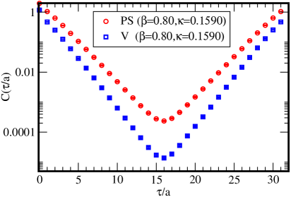
Figure 1: Correlation functions for the pseudoscalar (PS) and vector (V) mesons at ($\beta,\kappa$) $=$ ($0.80,0.1590$).

Figure 1 shows the correlation functions in the PS and vector meson channels at ($\beta,\kappa$) $=$ ($0.80,0.1590$). When extracting effective masses, instead of a simple ratio $C(\tau/a+1)/C(\tau/a)$ in Eq. (10), we utilized an alternative one that has not only the forward slope but also the backward slope of the correlator taken into account to achieve better accuracy: $[C(\tau/a+1)+C(\tilde{\tau}/a-1)]/[C(\tau/a)+C(\tilde{\tau}/a)]$, where the forward imaginary time in lattice units $\tau/a$ and the backward one $\tilde{\tau}/a$ are symmetric about $N_{\tau}/2$. The fitting is performed by using only larger time slices to omit the contributions of excited modes.

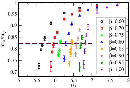
Figure 2: $m_{\mathrm{PS}}/m_{\mathrm{V}}$ for various combinations of the hopping parameter $\kappa$ and $\beta$.

$\beta$	$\kappa(m_{\mathrm{PS}}/m_{\mathrm{V}}=0.8232)$	$\kappa_{c}$
0.60	0.1764	0.1839(1)
0.70	0.1678	0.1728(1)
0.75	0.1629	0.1673(1)
0.80	0.1590	0.1627(1)
0.85	0.1549	0.1584(1)
0.90	0.1515	0.1546(0)
0.95	0.1490	0.1515(1)
1.00	0.1465	0.1489(1)

Table 1: Summary of the values of $\kappa$ consistent with $m_{\mathrm{PS}}/m_{\mathrm{V}}=0.8232$ and $\kappa_{c}$ for each $\beta$.

For details of the resulting masses, we refer the reader to tables 4 and 5 in the Appendix. In figure 2, we show the $m_{\mathrm{PS}}$-to-$m_{\mathrm{V}}$ ratio as a function of the inverse hopping parameter $1/\kappa$ for each $\beta$. We determine the value of $\kappa$ consistent with $m_{\mathrm{PS}}/m_{\mathrm{V}}=0.8232$ for each $\beta$ by linearly interpolating $3$ data near $m_{\mathrm{PS}}/m_{\mathrm{V}}=0.8232$. The results for ($\beta,\kappa$) are shown in table 1. Here, the statical errors of the $\kappa$ values on the line of $m_{\mathrm{PS}}/m_{\mathrm{V}}=0.8232$ are to be less than $2\%$ accuracy.

4.2 Mass renormalization

The PCAC mass can be read off from Eq. (19) using the calculated meson correlation functions. Figure 3 shows the PCAC mass as a function of $1/\kappa$ at fixed $\beta$, which gives the relation between the renormalized mass and bare mass of the quark. Here, for the difference operator in Eq. (19), we have considered not only the forward difference $\partial_{4}$ but also the backward difference $\tilde{\partial}_{4}$ (i.e., $\partial_{4}\rightarrow\frac{1}{2}(\partial_{4}+\tilde{\partial}_{4})$) to achieve better accuracy. For smaller values of $m_{\mathrm{PCAC}}$, we can fit them with the function of $(1/\kappa-1/\kappa_{c})$. We find the extrapolated value for $1/\kappa$ at $m_{\mathrm{PCAC}}=0$, which leads to $\kappa_{c}$. The values of $\kappa_{c}$ for each $\beta$ are summarized in table 1.

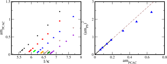
Figure 3: (Left) The hopping parameter dependence of $m_{\mathrm{PCAC}}$. Each color denotes the same value of $\beta$ as in Fig. 2. (Right) The PCAC mass dependence of the PS meson mass squared at $\beta=0.80$. The dashed line denotes the linear fitting-function by which we fit four data points in the small $am_{\mathrm{PCAC}}$ regime.

We also present the PS meson mass squared as a function of the PCAC mass as exemplary data ($\beta=0.80$) in lattice units in the right panel of Fig. 3. We can see that $m^{2}_{\mathrm{PS}}$ linearly depends on $m_{\mathrm{PCAC}}$ in the regime of smaller masses:

$$a^{2}m_{\mathrm{PS}}^{2}\propto am_{\mathrm{PCAC}},$$ (22)

which implies that the PCAC relation (or the Gell-Mann–Oakes–Renner relation for the PS meson mode) holds. Thus, $m_{\mathrm{PS}}\rightarrow 0$ in the limit of $m_{\mathrm{PCAC}}\rightarrow 0$.

Note that in two-color QCD it is known that the chiral symmetry can be restored in the chiral limit even at zero chemical potential. Instead of the spontaneous breaking of the chiral symmetry, the spontaneous breaking of the baryon charge symmetry occurs because of meson-baryon symmetry in two-color QCD Kogut:1999iv ; Furusawa:2020qdz .

4.3 Scale-setting function

Now we determine the relative scale of $a$ for several $\beta$ using the reference scale $w_{0}$ in the gradient flow method. First of all, we have generated the gauge configurations on $16^{3}\times 32$ on the line of constant physics. The resulting meson spectrum from the generated configurations is summarized in Table 2.

$\beta(\kappa)$	$am_{\mathrm{PS}}$	$m_{\mathrm{PS}}/m_{\mathrm{V}}$	$am_{\mathrm{PCAC}}$
0.60 (0.1764)	0.9075(11)	0.8336(50)	0.1482(3)
0.70 (0.1678)	0.7655(23)	0.8217(88)	0.1107(7)
0.75 (0.1629)	0.7216(29)	0.8260(49)	0.1073(5)
0.80 (0.1590)	0.6229(34)	0.8233(90)	0.08593(77)
0.85 (0.1549)	0.5748(29)	0.8179(80)	0.08240(62)
0.90 (0.1515)	0.5092(38)	0.8118(50)	0.07299(66)
0.95 (0.1490)	0.4349(42)	0.8207(75)	0.06206(60)
1.00 (0.1465)	0.4108(58)	0.8274(105)	0.06159(94)

Table 2: Summary of the values of $m_{\mathrm{PS}}$, $m_{\mathrm{PS}}/m_{\mathrm{V}}$, and $m_{\mathrm{PCAC}}$ for each $\beta$ on the line of constant physics.

Next, we have numerically solved the gradient flow by starting with the generated configurations and utilizing the Wilson gauge action for the gradient flow process. Finally, we have measured the expectation value of $t^{2}\langle E(t)\rangle$ in the range of $\beta=0.60-1.00$ using the clover-leaf definition for $G_{\mu\nu}$. Here, we have estimated the statistical errors using the Jackknife method.

Figure 4: Results for the dimensionless combination $t^{2}\langle E(t)\rangle$ and $td(t^{2}\langle E(t)\rangle)/dt$ as a function of the flow time in lattice units $t/a^{2}$. We plot the data for $0.60\leq\beta\leq 1.00$ and each color denotes the same value of $\beta$ as in Fig. 2. Two dashed lines, magenta and cyan, denote ${\cal T}$ or ${\cal W}=0.30$ and $0.50$, respetively.

Figure 4 shows the results for $t^{2}\langle E(t)\rangle$ and $tdt^{2}{\langle E(t)}/dt$ at each $\beta$. Here, ${\cal T}=0.30,0.50$ and ${\cal W}=0.30,0.50$ are also plotted as guiding lines of the reference scales in the left and right panels, respectively. We see that all reference scales for ${\cal T}$ and ${\cal W}$ are located in the approximately linear-scaling region of the observables.

	${\cal W}=0.30$	${\cal W}=0.50$
$\beta(\kappa)$	$w_{0}/a$	$w_{0}/a$
0.60 (0.1764)	0.6830(4)	0.8733(12)
0.70 (0.1678)	0.8219(15)	1.067(2)
0.75 (0.1629)	0.9205(21)	1.182(4)
0.80 (0.1590)	1.074(4)	1.360(6)
0.85 (0.1549)	1.240(7)	1.556(11)
0.90 (0.1515)	1.463(16)	1.791(20)
0.95 (0.1490)	1.781(29)	2.162(40)
1.00 (0.1465)	2.048(40)	2.462(59)

Table 3: The relation between $\beta$ and $w_{0}/a$ at ${\cal W}=0.30,0.50$.

Table 3 gives the value of $w_{0}/a$ for each $\beta$ at ${\cal W}=0.30$ and ${\cal W}=0.50$. To obtain the scale setting function around $T_{c}$, we utilize the smaller reference scale ${\cal W}=0.30$, which gives less statistical uncertainty, and find

$$\log(w_{0}/a)=-0.6469-1.045\beta+2.428\beta^{2}.$$ (23)

Here, we utilize $0.80\leq\beta\leq 1.00$ for the interpolation. To see the wider region of $\beta$, taking the lager reference scale ${\cal W}=0.50$ is better to avoid strong discretization errors that are inevitable for $w_{0}\ll a$. The best-fit function is expressed by

$$\log(w_{0}/a)=-0.3822-0.9212\beta+2.221\beta^{2}$$ (24)

for $0.60\leq\beta\leq 1.00$.

5 Results at finite temperature

We perform finite temperature simulations on the lattice with the size $N_{s}=32$ and $N_{\tau}=10$ using the same lattice action as the $T=0$ calculations. To determine the critical temperature on the line of constant physics, we set the parameter set of ($\beta,\kappa$) as shown in Table 1. We have sampled one configuration every $10$ trajectories and eventually produced $600$ configurations for each $\beta$. We observe the Polyakov loop and chiral condensate as well as the corresponding susceptibilities. Finally, we will estimate the pseudo-critical temperature from a peak position of the chiral susceptibility.

Following Eqs. (16), (17), (18) and (20), we calculate the Polyakov loop, the susceptibility of the Polyakov loop, the subtracted chiral condensate and the chiral susceptibility, respectively. Note here that we use $am_{\mathrm{PCAC}}$ for each $\beta$ in Table 2 in calculating the subtracted chiral condensate (18). The top panel of Fig. 5 depicts the Polyakov loop (red-circle) and the subtracted chiral condensate (black-square), while the bottom panel shows the chiral susceptibility on $32^{3}\times 10$ lattice. By scanning a range of $\beta=0.75-1.00$, we find that the Polyakov loop increases while the chiral condensate decreases in this regime. Although the susceptibility of the Polyakov loop is very noisy and we cannot find its peak, we can see a peak of the chiral susceptibility.

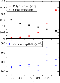
Figure 5: (Top) The Polyakov loop and the subtracted chiral condensate as a function of $\beta$. The lattice size is $32^{3}\times 10$. For easy seeing, we display the value of the Polyakov loop multiplied by a factor $10$. (Bottom) The chiral susceptibility as a function of $\beta$.

A peak at $\beta=0.95$ is shown in the bottom panel of Fig. 5. Here, we identify the value as a pseudo-critical $\beta$, i.e., $\beta_{c}$. It is very hard to determine the precise value of $\beta_{c}$ since we have to fix a value of $\kappa$ for each $\beta$ in such a way as to reproduce the reference value of $m_{\mathrm{PS}}/m_{\mathrm{V}}$.

We have also calculated the same quantities on $32^{3}\times 6$ and $32^{3}\times 8$. In these cases, however, we cannot find a clear peak of the susceptibility. The difficulty of the determination of $\beta_{c}$ might come from the weakness of the phase transition in two-color QCD. As for the order of phase transition in the SU(3) gauge theory, namely, quenched QCD, the chiral phase transition for probe quarks and color confinement, which are known to simultaneously occur, are of first-order. In $N_{f}=2$ massless three-color QCD, on the other hand, there remains a controversy about whether the chiral phase transition is described by the first- or second-order phase transition Pisarski:1983ms ; Aoki:2012yj . The SU(2) gauge theory or quenched two-color QCD is governed by the second-order phase transition Hirakida:2018uoy ; Berg:2016wfw ; Giudice:2017dor , since the smaller number of degrees of freedom weakens the phase transition. We expect that the $N_{f}=2$ two-color QCD undergoes a further weak phase transition or crossover even in the massless limit and that the peak of susceptibility must be even broader because of finite mass effects.

Finally, we translate the lattice parameters to the temperature normalized by the pseudo-critical temperature. The temperature on the lattice is defined by the inverse of the lattice extent in the Euclidean time direction,

$$T=\frac{1}{N_{\tau}a}.$$ (25)

We identify the pseudo-critical value as $\beta_{c}=0.95$ and $N_{\tau}=10$ by looking for the peak in the chiral susceptibility. Thus, we define the pseudo-critical temperature as $T_{c}=\frac{1}{N_{\tau}a(\beta_{c})}$. This definition of the pseudo-critical temperature includes the finite-volume effects, so that ideally we must study the thermodynamic limit $N_{s}\rightarrow\infty$ and continuum limit $N_{\tau}\rightarrow\infty$. In the present work, we take the same order of $N_{\tau}$ as $N_{s}$ and take this $T_{c}$ determined by the simulation in $N_{\tau}=10$ as the pseudo-critical temperature.

Combining with the scale setting function or Table 3, which gives the relation between $a$ and $\beta$, we can calculate $T/T_{c}$ for any values of $\beta$ and $N_{\tau}$. For instance, $\beta=0.80,N_{\tau}=8$ and $\beta=0.80,N_{\tau}=16$, where we have investigated the phase structure in the previous work Iida:2019rah , correspond to $T=0.79(2)(3)T_{c}$ and $T=0.39(1)(2)T_{c}$, respectively. Here, the first bracket denotes the statistical uncertainty coming from the statistical error of the $w_{0}/a$, while the second one shows the systematic uncertainty coming from the choice of the reference scale ${\mathcal{W}}=0.30$ or $0.50$. As we explained, there is unknown uncertainty from the determination of $\beta_{c}$, which will be addressed in future works.

6 Summary

In this paper, we have calculated the meson spectrum in two-color QCD using the Iwasaki gauge and $N_{f}=2$ Wilson fermion actions on $16^{3}\times 32$ lattice. We have reported a set of lattice parameters ($\kappa,\beta$) on the line of constant physics that satisfies $m_{\mathrm{PS}}/m_{\mathrm{V}}=0.8232$. Furthermore, we have obtained the scale setting function, which gives a relation between the lattice bare coupling constant $\beta$ and the lattice spacing, on the line of constant physics. To find the scale setting function, we have utilized the $w_{0}$-scale in the gradient flow method. It has given a precise scale setting function. We have also found the pseudo-critical temperature from the chiral susceptibility on $32^{3}\times 10$.

Using the results for the scale setting function and the pseudo-critical temperature, which is given by $\beta=0.95,N_{\tau}=10$, we can finally calculate the temperature scale for any $\beta$ and $N_{\tau}$ in $0.60\leq\beta\leq 1.00$. The temperature normalized by $T_{c}$ and the chemical potential normalized by $m_{\mathrm{PS}}$ would be helpful for a qualitative comparison among several proposed two-color QCD phase diagrams using different lattice actions Hands:2006ve ; Hands:2010gd ; Cotter:2012mb ; Makiyama:2015uwa ; Braguta:2016cpw ; Holicki:2017psk ; Boz:2019enj ; Iida:2019rah . Furthermore, it might be useful to see a comparison between the two-color and three-color QCD phase diagrams.

Appendix A Summary of masses

$\beta$	$\kappa$	$am_{\mathrm{PS}}$	$m_{\mathrm{PS}}/m_{\mathrm{V}}$	$am_{\mathrm{PCAC}}$	$\#$ of conf.	$\#$ of trj.
0.6000	0.1400	2.015(1)	0.9864(2)	1.219(4)	30	3000
0.6000	0.1500	1.767(1)	0.9755(7)	0.8348(20)	30	3000
0.6000	0.1600	1.499(2)	0.9540(9)	0.5336(26)	30	3000
0.6000	0.1700	1.184(2)	0.9101(56)	0.2850(13)	30	3000
0.6000	0.1750	0.9751(35)	0.8448(88)	0.1762(17)	30	3000
0.6000	0.1770	0.8755(17)	0.8145(61)	0.1354(3)	150	3000
0.6000	0.1780	0.8204(15)	0.7956(40)	0.1155(5)	300	6000
0.6000	0.1800	0.6805(18)	0.7252(108)	0.07519(67)	300	6000
0.7000	0.1400	1.832(1)	0.9832(4)	0.9513(24)	30	3000
0.7000	0.1500	1.533(1)	0.9643(16)	0.5875(15)	30	3000
0.7000	0.1550	1.366(3)	0.9481(13)	0.4360(16)	30	3000
0.7000	0.1600	1.173(3)	0.9277(47)	0.3005(23)	30	3000
0.7000	0.1650	0.9386(21)	0.8711(52)	0.1763(9)	120	6000
0.7000	0.1670	0.8236(30)	0.8491(50)	0.1301(7)	100	5000
0.7000	0.1680	0.7490(16)	0.8157(106)	0.1056(8)	90	4500
0.7000	0.1690	0.6734(24)	0.7861(81)	0.08360(53)	120	6000
0.7000	0.1700	0.5905(30)	0.7227(222)	0.06222(91)	120	6000
0.7500	0.1625	0.7527(15)	0.8311(79)	0.1165(7)	170	8500
0.7500	0.1630	0.7165(14)	0.8291(56)	0.1053(7)	120	6000
0.7500	0.1635	0.6761(12)	0.7928(70)	0.09323(77)	180	9000
0.7500	0.1640	0.6345(28)	0.7764(108)	0.08071(78)	120	6000
0.7500	0.1645	0.5833(20)	0.7734(89)	0.06762(139)	120	6000
0.8000	0.1300	1.887(2)	0.9893(3)	1.076(3)	30	3000
0.8000	0.1400	1.550(3)	0.9768(8)	0.6506(30)	30	3000
0.8000	0.1450	1.364(2)	0.9658(23)	0.4785(18)	30	3000
0.8000	0.1500	1.159(3)	0.9422(20)	0.3231(23)	30	3000
0.8000	0.1550	0.9076(32)	0.9072(83)	0.1866(16)	30	3000
0.8000	0.1570	0.7773(48)	0.8644(48)	0.1367(17)	60	3000
0.8000	0.1590	0.6229(34)	0.8233(90)	0.08593(77)	120	6000
0.8000	0.1600	0.5240(32)	0.7577(120)	0.06302(72)	130	6500

Table 4: Summary of pseudoscalar (PS), vector (V) and partially conserved axial current (PCAC) masses for $\beta=0.60,0.70,0.75,0.80$, using $16^{3}\times 32$ lattice. The total numbers of configurations and of trajectories are also shown.

$\beta$	$\kappa$	$am_{\mathrm{PS}}$	$m_{\mathrm{PS}}/m_{\mathrm{V}}$	$am_{\mathrm{PCAC}}$	$\#$ of conf.	$\#$ of trj.
0.8500	0.1547	0.5900(24)	0.8248(66)	0.08688(45)	140	7000
0.8500	0.1550	0.5648(33)	0.8320(79)	0.07935(71)	120	6000
0.8500	0.1555	0.5095(32)	0.7998(92)	0.06585(97)	120	6000
0.8500	0.1556	0.5062(36)	0.7770(100)	0.06431(56)	120	6000
0.8500	0.1560	0.4640(18)	0.7850(109)	0.05459(62)	200	10000
0.8500	0.1565	0.4158(66)	0.7354(106)	0.04306(115)	120	6000
0.9000	0.1300	1.591(3)	0.9874(4)	0.7585(32)	30	3000
0.9000	0.1400	1.191(3)	0.9666(16)	0.3959(19)	30	3000
0.9000	0.1500	0.6313(44)	0.8822(69)	0.1128(17)	30	3000
0.9000	0.1510	0.5553(35)	0.8444(101)	0.08537(116)	60	3000
0.9000	0.1520	0.4610(30)	0.8141(124)	0.06219(136)	150	7500
0.9000	0.1525	0.4167(52)	0.7762(103)	0.04920(99)	150	7500
0.9000	0.1530	0.3638(59)	0.7145(166)	0.03724(67)	120	6000
0.9500	0.1485	0.4757(36)	0.8481(89)	0.07469(57)	170	8500
0.9500	0.1490	0.4349(42)	0.8207(75)	0.06206(60)	190	9500
0.9500	0.1495	0.3858(46)	0.8069(63)	0.04809(115)	160	8000
0.9500	0.1500	0.3369(90)	0.7210(212)	0.03723(107)	200	10000
1.000	0.1300	1.312(4)	0.9869(8)	0.5505(17)	30	3000
1.000	0.1350	1.080(7)	0.9781(20)	0.3764(27)	30	3000
1.000	0.1400	0.8343(62)	0.9544(42)	0.2339(14)	30	3000
1.000	0.1450	0.5163(59)	0.8941(105)	0.09890(239)	30	3000
1.000	0.1460	0.4444(51)	0.8596(78)	0.07472(137)	60	3000
1.000	0.1465	0.4108(58)	0.8274(105)	0.06159(94)	170	8500
1.000	0.1470	0.3690(62)	0.7889(109)	0.04959(158)	120	6000
1.000	0.1475	0.3524(68)	0.7324(166)	0.03512(154)	120	6000

Table 5: Summary of pseudoscalar (PS), vector (V), and partially conserved axial current (PCAC) masses measured on the lattice $16^{3}\times 32$ for $\beta=0.85,0.90,0.95,1.00$. The total numbers of configurations and of trajectories are also shown.

- (1) A. Nakamura, “Quarks and Gluons at Finite Temperature and Density,” Phys. Lett. 149B (1984) 391.
- (2) S. Hands, J. B. Kogut, M. P. Lombardo and S. E. Morrison, “Symmetries and spectrum of SU(2) lattice gauge theory at finite chemical potential”, Nucl. Phys. B 558 (1999) 327, [hep-lat/9902034].
- (3) R. Aloisio, V. Azcoiti, G. Di Carlo, A. Galante and A. F. Grillo, “Fermion condensates in two colors finite density QCD at strong coupling,” Phys. Lett. B 493 (2000) 189, [hep-lat/0009034].
- (4) S. Hands, I. Montvay, S. Morrison, M. Oevers, L. Scorzato and J. Skullerud, “Numerical study of dense adjoint matter in two color QCD,” Eur. Phys. J. C 17 (2000) 285, [hep-lat/0006018].
- (5) S. Muroya, A. Nakamura and C. Nonaka, “Monte Carlo study of two color QCD with finite chemical potential: Status report of Wilson fermion simulation,” Nucl. Phys. Proc. Suppl. 94 (2001) 469, [hep-lat/0010073].
- (6) J. B. Kogut, D. Toublan and D. K. Sinclair, “Diquark condensation at nonzero chemical potential and temperature,” Phys. Lett. B 514 (2001) 77, [hep-lat/0104010].
- (7) J. B. Kogut, D. K. Sinclair, S. J. Hands and S. E. Morrison, “Two color QCD at nonzero quark number density, Phys. Rev. D 64 (2001) 094505, [hep-lat/0105026].
- (8) J. B. Kogut, D. Toublan and D. K. Sinclair, “The Phase diagram of four flavor SU(2) lattice gauge theory at nonzero chemical potential and temperature, Nucl. Phys. B 642 (2002) 181, [hep-lat/0205019].
- (9) S. Muroya, A. Nakamura and C. Nonaka, “Behavior of hadrons at finite density: Lattice study of color SU(2) QCD,” Phys. Lett. B 551 (2003) 305, [hep-lat/0211010].
- (10) J. B. Kogut, D. Toublan and D. K. Sinclair, “The PseudoGoldstone spectrum of two color QCD at finite density, Phys. Rev. D 68 (2003) 054507, [hep-lat/0305003].
- (11) S. Hands, S. Kim and J. I. Skullerud, “Deconfinement in dense 2-color QCD,” Eur. Phys. J. C 48 (2006) 193, [hep-lat/0604004].
- (12) S. Hands, S. Kim and J. I. Skullerud, “A Quarkyonic Phase in Dense Two Color Matter?,” Phys. Rev. D 81 (2010) 091502, [arXiv:1001.1682 [hep-lat]].
- (13) S. Cotter, P. Giudice, S. Hands and J. I. Skullerud, “Towards the phase diagram of dense two-color matter, Phys. Rev. D 87 (2013) 034507, [arXiv:1210.4496 [hep-lat]].
- (14) T. Boz, S. Cotter, L. Fister, D. Mehta and J. I. Skullerud, “Phase transitions and gluodynamics in 2-colour matter at high density, Eur. Phys. J. A 49 (2013) 87, [arXiv:1303.3223 [hep-lat]].
- (15) T. Makiyama et al., “Phase structure of two-color QCD at real and imaginary chemical potentials; lattice simulations and model analyses,” Phys. Rev. D 93 (2016) 014505, [arXiv:1502.06191 [hep-lat]].
- (16) V. V. Braguta, E.-M. Ilgenfritz, A. Y. Kotov, A. V. Molochkov and A. A. Nikolaev, “Study of the phase diagram of dense two-color QCD within lattice simulation,” Phys. Rev. D 94 (2016) 114510, [arXiv:1605.04090 [hep-lat]].
- (17) L. Holicki, J. Wilhelm, D. Smith, B. Wellegehausen and L. von Smekal, “Two-colour QCD at finite density with two flavours of staggered quarks,” PoS LATTICE 2016 (2017) 052, [arXiv:1701.04664 [hep-lat]].
- (18) V. G. Bornyakov, V. V. Braguta, E. M. Ilgenfritz, A. Y. Kotov, A. V. Molochkov and A. A. Nikolaev, “Observation of Deconfinement in a Cold Dense Quark Medium,” JHEP 03 (2018), 161 [arXiv:1711.01869 [hep-lat]].
- (19) N. Y. Astrakhantsev, V. G. Bornyakov, V. V. Braguta, E. M. Ilgenfritz, A. Y. Kotov, A. A. Nikolaev and A. Rothkopf, “Lattice Study of Static Quark-Antiquark Interactions in Dense Quark Matter,” JHEP 05 (2019), 171 [arXiv:1808.06466 [hep-lat]].
- (20) T. Boz, O. Hajizadeh, A. Maas and J. I. Skullerud, “Finite-Density Gauge Correlation Functions in Qc2D,” Phys. Rev. D 99 (2019) no.7, 074514 [arXiv:1812.08517 [hep-lat]].
- (21) J. Wilhelm, L. Holicki, D. Smith, B. Wellegehausen and L. von Smekal, “Continuum Goldstone Spectrum of Two-Color QCD at Finite Density with Staggered Quarks,” Phys. Rev. D 100 (2019) no.11, 114507 [arXiv:1910.04495 [hep-lat]].
- (22) K. Iida, E. Itou and T. G. Lee, “Two-Colour QCD Phases and the Topology at Low Temperature and High Density,” JHEP 2001 (2020) 181 [arXiv:1910.07872 [hep-lat]].
- (23) T. Boz, P. Giudice, S. Hands and J. I. Skullerud, “Dense Two-Color QCD Towards Continuum and Chiral Limits,” Phys. Rev. D 101 (2020) no.7, 074506 [arXiv:1912.10975 [hep-lat]].
- (24) V. G. Bornyakov, V. V. Braguta, A. A. Nikolaev and R. N. Rogalyov, “Effects of Dense Quark Matter on Gluon Propagators in Lattice Qc2D,” [arXiv:2003.00232 [hep-lat]].
- (25) P. V. Buividovich, D. Smith and L. von Smekal, “Electric conductivity in finite-density SU(2) lattice gauge theory with dynamical fermions,” [arXiv:2007.05639 [hep-lat]].
- (26) N. Y. Astrakhantsev, V. V. Braguta, E. M. Ilgenfritz, A. Y. Kotov and A. A. Nikolaev, “Lattice study of thermodynamic properties of dense QC2D,” [arXiv:2007.07640 [hep-lat]].
- (27) T. T. Takahashi and Y. Kanada-En’yo, “Hadron-Hadron Interaction from Lattice QCD,” Phys. Rev. D 82 (2010), 094506 [arXiv:0912.0691 [hep-lat]].
- (28) M. Caselle, A. Nada and M. Panero, “Hagedorn Spectrum and Thermodynamics of and Yang-Mills Theories,” JHEP 07 (2015), 143 [arXiv:1505.01106 [hep-lat]].
- (29) B. A. Berg and D. A. Clarke, “Deconfinement, gradient and cooling scales for pure SU(2) lattice gauge theory,” Phys. Rev. D 95 (2017) 094508, [arXiv:1612.07347 [hep-lat]].
- (30) P. Giudice and S. Piemonte, “Improved thermodynamics of SU(2) gauge theory,” Eur. Phys. J. C 77 (2017) 821, [arXiv:1708.01216 [hep-lat]].
- (31) T. Hirakida, E. Itou and H. Kouno, “Themodynamics for pure SU() gauge theory using gradient flow,” PTEP 2019 (2019) no.3, 033B01 [arXiv:1805.07106 [hep-lat]].
- (32) T. Furusawa, Y. Tanizaki and E. Itou, “Finite-Density Massless Two-Color QCD at Isospin Roberge-Weiss Point and ‘T Hooft Anomaly,” [arXiv:2005.13822 [hep-th]]. To appear in Physical Review Research
- (33) J. B. Kogut, M. A. Stephanov and D. Toublan, “On Two Color QCD with Baryon Chemical Potential,” Phys. Lett. B 464 (1999) 183 [hep-ph/9906346].
- (34) P. Adhikari, S. B. Beleznay and M. Mannarelli, “Finite Density Two Color Chiral Perturbation Theory Revisited,” Eur. Phys. J. C 78 (2018) no.6, 441 [arXiv:1803.00490 [hep-th]].
- (35) R. Contant and M. Q. Huber, “Dense Two-Color QCD from Dyson-Schwinger Equations,” Phys. Rev. D 101 (2020) no.1, 014016 [arXiv:1909.12796 [hep-ph]].
- (36) R. Sommer, “A New way to set the energy scale in lattice gauge theories and its applications to the static force and alpha-s in SU(2) Yang-Mills theory,” Nucl. Phys. B 411 (1994) 839, [hep-lat/9310022].
- (37) S. Necco and R. Sommer, “The N(f) = 0 heavy quark potential from short to intermediate distances,” Nucl. Phys. B 622 (2002) 328, [hep-lat/0108008].
- (38) M. Luscher, “Trivializing maps, the Wilson flow and the HMC algorithm,” Commun. Math. Phys. 293 (2010) 899, [arXiv:0907.5491 [hep-lat]].
- (39) M. Luscher and P. Weisz, “Perturbative analysis of the gradient flow in non-abelian gauge theories,” JHEP 1102 (2011) 051, [arXiv:1101.0963 [hep-th]].
- (40) M. Lüscher, “Properties and uses of the Wilson flow in lattice QCD,” JHEP 1008 (2010) 071, Erratum: [JHEP 1403 (2014) 092], [arXiv:1006.4518 [hep-lat]].
- (41) S. Borsanyi et al., “High-precision scale setting in lattice QCD,” JHEP 1209 (2012) 010, [arXiv:1203.4469 [hep-lat]].
- (42) Y. Iwasaki, “Renormalization Group Analysis of Lattice Theories and Improved Lattice Action: Two-Dimensional Nonlinear O(N) Sigma Model,” Nucl. Phys. B 258 (1985) 141;
- (43) Y. Iwasaki, “Renormalization Group Analysis of Lattice Theories and Improved Lattice Action. II. Four-dimensional non-Abelian SU(N) gauge model,” arXiv:1111.7054 [hep-lat].
- (44) S. Duane, A. D. Kennedy, B. J. Pendleton and D. Roweth, “Hybrid Monte Carlo,” Phys. Lett. B195 (1987) 216.
- (45) S. A. Gottlieb, W. Liu, D. Toussaint, R. L. Renken and R. L. Sugar, “Hybrid Molecular Dynamics Algorithms for the Numerical Simulation of Quantum Chromodynamics, Phys. Rev. D35 (1987) 2531.
- (46) W. Pauli, “On the conservation of the lepton charge,” Nuovo Cimento 6 (1957) 205.
- (47) F. Gürsey, “Relation of charge independence and baryon conservation to Pauli’s transformation,” Nuovo Cimento 7 (1958) 411.
- (48) R. Sommer, “Scale setting in lattice QCD,” PoS LATTICE2013 (2014), 015 doi:10.22323/1.187.0015 [arXiv:1401.3270 [hep-lat]].
- (49) M. Bochicchio, L. Maiani, G. Martinelli, G. C. Rossi and M. Testa, “Chiral Symmetry on the Lattice with Wilson Fermions,” Nucl. Phys. B 262 (1985) 331.
- (50) S. Itoh, Y. Iwasaki, Y. Oyanagi and T. Yoshie, “Hadron Spectrum in Quenched QCD on a 12**3 X 24 Lattice With Renormalization Group Improved Lattice SU(3) Gauge Action,” Nucl. Phys. B 274 (1986) 33.
- (51) S. Aoki, “Phase structure of lattice QCD with Wilson fermion at finite temperature,” Nucl. Phys. Proc. Suppl. 60A (1998) 206, [hep-lat/9707020].
- (52) L. Giusti, F. Rapuano, M. Talevi and A. Vladikas, “The QCD chiral condensate from the lattice,” Nucl. Phys. B 538 (1999) 249, [hep-lat/9807014].
- (53) T. Umeda et al. [WHOT-QCD Collaboration], “Thermodynamics in 2+1 flavor QCD with improved Wilson quarks by the fixed scale approach, PoS LATTICE 2012 (2012) 074, [arXiv:1212.1215 [hep-lat]].
- (54) M. Hayakawa, K. I. Ishikawa, S. Takeda, M. Tomii and N. Yamada, “Lattice Study on quantum-mechanical dynamics of two-color QCD with six light flavors,” Phys. Rev. D 88 (2013) no.9, 094506 [arXiv:1307.6696 [hep-lat]].
- (55) T. Iritani, E. Itou and T. Misumi, “Lattice study on QCD-like theory with exact center symmetry,” JHEP 1511 (2015) 159, [arXiv:1508.07132 [hep-lat]].
- (56) Z. Fodor and S. D. Katz, “The Phase diagram of quantum chromodynamics,” [arXiv:0908.3341 [hep-ph]].
- (57) R. D. Pisarski and F. Wilczek, “Remarks on the Chiral Phase Transition in Chromodynamics,” Phys. Rev. D 29 (1984), 338-341
- (58) S. Aoki, H. Fukaya and Y. Taniguchi, “Chiral Symmetry Restoration, Eigenvalue Density of Dirac Operator and Axial U(1) Anomaly at Finite Temperature,” Phys. Rev. D 86 (2012), 114512 [arXiv:1209.2061 [hep-lat]].