Light element () production from spontaneous ternary fission of 252Cf
Abstract
The yields of light elements () obtained from spontaneous ternary fission of 252Cf are treated within a nonequilibrium approach, and the contribution of unstable nuclei and excited bound states is taken into account. These light cluster yields may be used to probe dense matter, and to infer in-medium corrections. Continuum correlations are calculated from scattering phase shifts using the Beth-Uhlenbeck formula, and the effect of medium modification is estimated. The relevant distribution is reconstructed from the measured yields of isotopes. This describes the state of the nucleon system at scission and cluster formation, using only three Lagrange parameters which are the nonequilibrium counterparts of the temperature and chemical potentials, as defined in thermodynamic equilibrium. We concluded that a simple nuclear statistical equilibrium model neglecting continuum correlations and medium effects is not able to describe the measured distribution of H and He isotopes. Moreover, the freeze-out concept may serve as an important ingredient to the nonequilibrium approach using the relevant statistical operator concept.
pacs:
21.65.-f, 21.60.Jz, 25.70.Pq, 26.60.KpI Introduction
Thermal neutron induced and spontaneous ternary fission is a process in which the emission of two medium-mass fragments is accompanied by equatorially emitted light particles and clusters formed in the neck region at the time of scission, see [1] ; [2] ; [3] and references therein. Data for cluster yields obtained from ternary fission experiments with thermal neutrons are shown, e.g., in Koester ; Koestera ; KoesterPhD . In particular, data for the ternary fission yields of 241Pu(,f) are presented. An interpretation of the Koester et al. data Koester was given in Ref. Sarah , where a suppression of the yields of the larger clusters is found, due to cluster formation kinetics. Also, ternary fission has been observed from other actinides such as 239Pu, 233U, 235U, and 245Cm. For more recent work on ternary fission see Zagrebaev ; Artemenkov ; Holmvall ; Chuvilskaya ; Wollersheim .
Different approaches have been employed to interpret these data, see Koestera , and often a Boltzmann distribution has been used. An interpolation formula has been presented in Valskii2 which describes the general behavior of the measured yields but cannot explain the details of the observed distributions. More fundamentally, the use of a Boltzmann distribution as known from thermodynamic equilibrium with parameters temperature and chemical potentials remains unfounded. However, the signatures of binding energies and degeneracy of the isotopes according to the Boltzmann distribution are clearly seen in the observed yields.
In this paper we report on investigations of the yields of equatorial emission of isotopes during ternary spontaneous fission of 252Cf. We are interested in a better understanding of cluster formation and the fate of correlations in low density, low-temperature, expanding nuclear matter. This nonequilibrium evolution can be described using the method of the nonequilibrium statistical operator (NSO) NSO . It is based on information-theoretical concepts which is also the basis of equilibrium statistical physics. We include different processes which describe the dynamical evolution of the system. In particular, we include the decay from other unstable nuclei (feeding), the inclusion of excited states (including continuum correlations), and medium effects. For this, a quantum statistical approach is used.
Our main goal is to shed some more light into the properties of dense nuclear matter, namely, to understand how to improve the simple model of nuclear statistical equilibrium (NSE) by including continuum correlations and in-medium effects, and how well the nucleon density at the time of onset of cluster formation can be determined. We discuss the apparent suppression of yield for some exotic isotopes and the relation to thermodynamic quantities.
The paper is organized as follows: in Section II, we collect available data on ternary spontaneous fission of 252Cf concerning the production of the lightest elements H and He. In Sec.III, the theoretical formalism used in the work, based on information theory, will be described. Section IV analyses different numerical calculations that go beyond the ideal gas description considering continuum correlations and in-medium effects. The use of a local density approximation is discussed in Section V, and finally in Section VI, some final remarks, namely, the relation to thermodynamics, are drawn.
II Experimental data
A number of experimental investigations of the spontaneous fission of 252Cf have been performed by different groups, see KoesterPhD and references given there. It has been demonstrated that 252Cf(sf) emits -particles per fission Rai68 ; Wil85 . Usually, the yields of other light elements produced from ternary fission are normalized to the final yield of 4He (), which is fixed to . More precisely, we consider here the ratios of yields relative to the final yield of -particles.
In Ref. KoesterPhDtab , the author performed a compilation of results for ternary fission data, taken from the literature. There, consistent experimental results are presented for the 1H () and 2H () yields, as well as for the 8He ones. However, the values for the yield of 3H (), and also of 6He, are quite different. These data have been used also in a more recent publication Valskii2 , where the yields for the H isotopes are from Ref. Whe67 , and for the He isotopes, the yields are according Ref. Dlo92 .
| isotope | ||||||||||||||
| - | - | - | (1.25) | - | - | 0.806219 | - | - | 1.28018 | - | 1.25052 | - | 1.30556 | |
| - | - | - | (-2.8) | - | - | -2.19217 | - | - | -3.18741 | - | -3.1107 | - | -3.00665 | |
| - | - | - | (-15.8) | - | - | -17.7023 | - | - | -16.5882 | - | -16.7538 | - | -16.6463 | |
| 1n | 1 | 0 | - | 0.65e6 | 0 | 2 | 2.572e8 | - | - | 1.084e6 | - | 1.647e6 | - | 954222 |
| 1H | 1 | 1 | 160(20) | 19.4 | 0 | 2 | 1.136 | - | - | 30.8231 | - | 30.096 | - | 27.625 |
| 2H | 2 | 1 | 63(3) | 37.5 | 1.112 | 3 | 5.012 | 2.224 | 1 | 61.6143 | 0.98 | 61.579 | 0.98 | 63.004 |
| 3Hf | 3 | 1 | 950(90) | 591 | 2.827 | 2 | 950 | - | - | 951.351 | - | 951.34 | - | 950.06 |
| 3H | 3 | 1 | - | - | 2.827 | 2 | (950) | 6.257 | 1 | 829.985 | 0.99 | 943.12 | 0.99 | 938.91 |
| 4H | 4 | 1 | - | - | 1.720 | 5 | (52.95 ) | -1.6 | 1.473 | 121.366 | 0.0606 | 8.2191 | 0.0606 | 11.154 |
| 3He | 3 | 2 | - | 0.0095 | 2.573 | 2 | 1.624e-6 | - | 1 | 0.012984 | 0.988 | 0.00933 | 0.988 | 0.01511 |
| 4Hef | 4 | 2 | 10000 | 10028 | 7.073 | 1 | 10000 | - | - | 10000 | - | 10000 | - | 10000 |
| 4He | 4 | 2 | 8264(341) | - | 7.073 | 1 | (10000) | 20.577 | 1 | 7920.86 | 1 | 8454.0 | 1 | 8256.7 |
| 5He | 5 | 2 | 1736(274) | 2600 | 5.512 | 4 | (1487) | -0.735 | 1 | 2072.8 | 0.7044 | 1540.9 | 0.6596 | 1733.9 |
| 6Hef | 6 | 2 | 270(30) | 369 | 4.878 | 1 | 270 | - | - | 280.724 | - | 280.6 | - | 270.02 |
| 6He | 6 | 2 | 223(26) | - | 4.878 | 1 | (270) | 0.975 | 1 | 215.488 | 0.9453 | 222.4 | 0.6961 | 223.16 |
| 7He | 7 | 2 | 47(9) | 128 | 4.123 | 4 | (53.76) | -0.410 | 1 | 65.2355 | 0.821 | 58.16 | 0.3988 | 46.863 |
| 8Hef | 8 | 2 | 25(5) | 30.6 | 3.925 | 1 | 25 | - | - | 12.8212 | - | 13.58 | - | 25.110 |
| 8He | 8 | 2 | 25(5) | - | 3.925 | 1 | (25) | 2.125 | 1 | 11.9324 | 0.9783 | 13.32 | 0.9783 | 24.513 |
| 9He | 9 | 2 | - | - | 3.349 | 2 | (0.8335) | -1.25 | 1 | 0.88875 | 0.2604 | 0.258 | 0.2604 | 0.59706 |
| 8Be | 8 | 4 | 10(6) | 15.2 | 7.062 | 1 | (0.2101) | -0.088 | 1.49 | 4.70862 | 1.07 | 2.544 | 1.07 | 5.0427 |
In Table 1 we collect some experimental results denoted as . For 1H and 2H, we give the values of Whe67 . For 3H, 4He, 5He, 6He, 7He, 8He, we take the values from Refs. Wollersheim ; Wollersheim1 where also the errors are given. Note that the long-living isotopes 6He and 8He which are unstable with respect to decay are stable with respect to strong interaction and are observed in the experiments. In addition to the final yields seen in the experiments, denoted by the superscript at the stable nucleus, we give also primary yields of short-living, particle unstable nuclei which can contribute to the yields of the observed nuclei. The final yields are related to the primary yields as . Analyzing the energy spectra, for 252Cf(sf) the formation of 5He and 7He has been determined Wollersheim , and the ratios of primary yields and have been reported. For 8Be, the value 10 was found for the primary yield in Jesinger05 .
For 252Cf the multiplicity of protons emitted in ternary fission is reported to be [2] . This corresponds to an experimental yield relative to the yield of -particles. Also prompt neutron emission has been measured, for a recent work see Chietera18 . The fractional percentage of ternary fission ”scission” neutrons has been determined to be Vorobyev ; Stuttge . In Ref. Stuttge a temperature of MeV has been used. A very recent measurement of the total neutron multiplicity in 252Cf fission is Hansell . This leads to a scission neutron multiplicity of that corresponds to an experimental yield relative to the yield of -particles.
As pointed out in Ref. Mutterer08 , experimental studies at low energy of ternary-particle-unstable nuclei producing particles are still scarce, and the data are not very consistent. The ratio 6Hef/4Hef was reconsidered in Mutterer08 , and a Gaussian fit above 9 MeV energy gives the value .
An interpolation formula has been presented in Ref. Valskii2 and compared to measured data (Whe67 for H and Dlo92 for He isotopes). Parameter values for quantities similar to the temperature ( MeV), the neutron chemical potential ( MeV) and the proton chemical potential ( MeV) have been fitted, and are also shown in Table 1 together with the yields Valskii2 , which are calculated with the Valski interpolation formula. To explain the yields observed from ternary fission of 252Cf(sf), Boltzmann-like distributions are used. These contain the binding energy and the ground-state degeneracy of nuclei nuclei which are also shown in Table 1. The remaining columns will be discussed in Sections III and IV below.
III Information theoretical description of the distribution of cluster yields
Information theory considers the problem of reconstructing a distribution if some information about the ensemble is given. The most probable distribution is obtained from the maximum of information entropy if some averages of of the system properties are given. From the maximum of information entropy, a Gibbs distribution is obtained with Lagrange parameters which are determined self-consistently, by describing the averages. In this section we consider whether it is possible to reconstruct the distribution of yields with only a limited amount of information about the system. This approach is well-known from equilibrium thermodynamics where the averages of energy and particle numbers of the conserved components are given to define the grand canonical ensemble, and the Lagrange parameters occurring in the equilibrium ensemble are related to the temperature and the chemical potentials.
Within the method of the nonequilibrium statistical operator (NSO) NSO , at a given time the relevant statistical operator is constructed from this maximum entropy principle, and the corresponding Lagrange parameters become functions of time. The statistical operator describing the nonequilibrium evolution of the system follows as
| (1) |
which solves the Liouville-von Neumann equation, with the system Hamiltonian given in Eq. (2). Kinetic equations as well as hydrodynamic equations can be derived within this approach.
We discuss the construction of the relevant statistical operator which is a ingredient to describe the nonequilibrium process. As relevant observables, we consider the averages of neutron number and proton number, as well as the Hamiltonian
| (2) |
which describes the interaction of nucleons, , with an external potential and the nucleon-nucleon interaction ; the quantum number denotes the wave vector and spin of the nucleon with kinetic energy . Averages are going to be calculated with the correspondent relevant operator
| (3) |
where is the relevant partition function, denotes the particle number of neutrons/protons, and the Lagrange multipliers are going to be eliminated by the known informations, such as internal energy and particle densities of the system.
The solution of this many-particle problem is not simple and needs some approximations, such as replacing the Hamiltonian by a more simple model which can be solved. Such simple model Hamiltonians are the ideal nucleon gas or the mean-field approximation, where the Hamiltonian describes a noninteracting system of quasiparticles. We are interested in the formation of bound states so that, in a first approximation, we consider the ideal energy functional
| (4) |
with the center of mass momentum for the cluster , is the average nucleon mass. This model Hamiltonian describes the nucleon system as an ideal mixture of non-interacting free nucleons and nuclei. We allow for reactions between the different components so that the number of each component is not conserved but only the total number of neutrons and protons in the system. This approximation can be applied in the low-density case where the interaction between the constituents of the nuclear system becomes weak. The Lagrange parameters in (3) calculated to reproduce the observed distribution with the model Hamiltonian (4), are denoted by , respectively.
The problem to eliminate the Lagrange multipliers by the given averages of internal energy and particle number densities is well known from statistical physics and leads to the Fermi/Bose distribution. Before we discuss the corresponding results, we emphasize that initially we are discussing only the parametrization of the measured yields, using information about the observed nuclei such as ground state binding energy and degeneracy.
The obtained Lagrange parameters should not be interpreted as thermodynamic quantities like temperature and chemical potentials for
several reasons:
(i) The energy functional is only an approximation. The full energy functional should also include excited states and interactions. The full information about the Hamiltonian of the system leads to the quantum statistical approach.
(ii) Fission is a nonequilibrium process and is not described by an equilibrium distribution.
We have to include also the dynamical information which is described by the full Hamiltonian
and contains the information on the final distribution measured in the experiment as well as information of the distribution in the past , see Eq. (1).
This leads to the so-called relevant distribution which depends on the time ,
and the evolution of the distribution with time described by generalized reaction kinetics NSO .
We will not discuss how the evolution of the system follows from the solution of (1)
but use instead the simple concept of the freeze-out approximation.
This means that the relevant distribution is given by thermodynamic equilibrium up to the freeze-out time. After that,
the relevant distribution evolves according to reaction kinetics as described by the decay of excited states.
The different versions of shown in Table 1 correspond to different model Hamiltonians as an approximation to the nucleon Hamiltonian (2).
(iii) The system to be described is not homogeneous nuclear matter as in thermodynamic equilibrium but is inhomogeneous.
A local density approximation is problematic. In addition, the relation between the Lagrange parameters and the thermodynamic quantities,
in particular the densities , is not the relation between temperature, chemical potentials and density
as known from non-interacting, ideal quantum gases but is more complex. Our aim is to find arguments to infer the density from the data.
The information of the properties of the observed nuclei, see Tab. 1, leads to the Boltzmann-like distribution (nondegenerate case)
| (5) |
Because we don’t know the prefactor we consider only the ratio , i.e., the isotope yield relative to the final yield of particles. Following convention, the final yield of the particles is fixed as .
We infer the Lagrange parameter values based on the information about the observed final nuclei by minimizing the sum over the relative square deviation . For instance, considering the four lightest and most abundant isotopes, i.e. the yield ratios of 3Hf, 4Hef, 6Hef, and 8Hef, we determine the values of the three Lagrange parameters MeV, MeV, MeV. The values for the corresponding yields (we drop the index ) is shown in Table 1.
This approach is similar to that used in the Albergo determination of temperature and chemical potentials from the observed yields of nucleons and nuclei from heavy ion collisions Albergo . However, we cannot identify the Lagrange parameters with the thermodynamic parameters temperature and chemical potential of the nuclear system because, and as stated above, the ideal energy functional (4) considers only the ground states of the nuclei, and the interaction between the nucleons/nuclei is neglected. In addition, the correct nonequilibrium distribution is given by (1) which coincides with only in thermodynamic equilibrium.
Evidently, our first approach which relates the final distribution to the binding energies of nuclei and their degeneracies is not sufficient. There are further unstable nuclei and excited states which should be taken into account. In addition to the stable isotopes 1H, 2H, 3He, 4He we have 6He and 8He which are unstable with respect to weak processes (-decay) but have a sufficiently long half-life so that they are observed like stable nuclei. Other isotopes such as 4H, 5He, 7He, 9He, 8Be are unstable with respect to the strong interaction and decay immediately so that these primary nuclei are not detected as final yields. They should appear in the relevant distribution if the model Hamiltonian (4) contains the sum over all bound states. We have calculated the expected yields of the unstable isotopes using the Lagrange parameters . These are given in Tab. 1, col. , in italic parentheses. We conclude that an essential part of clustering is found within these unstable nuclei.
This problem, that also the formation of unstable nuclei are expected, is solved by taking into account that the observed distribution are not equilibrium distributions but the result of a time evolution described by (1). To solve this in a simple approximation, we assume a freeze-out scenario. Up to the freeze-out time , only the information about energy density and particle number density is sufficient to describe the state of the system. The relevant distribution (3) can be used to describe the system.
After this, a more detailed description of the system is necessary where the occupation numbers of quasiparticle states of the components are relevant, the corresponding Lagrange parameters are the distribution functions. This stage of evolution is described by reaction kinetics, unstable nuclei decay that feed the states of observed stable nuclei. The primary distribution, described by the relevant statistical operator and the yields , is transformed to the yields of detected nuclei denoted as feeding in Section II, for instance , etc.
Another consideration is the inclusion of excited states of nuclei to characterize the relevant distribution, see the data tables in Ref. nuclei . Excited states contribute to the statistical weight of an isotope. For instance, the isotope 4H has an excited state at 0.31 MeV with a degeneracy factor 3. Assuming that this excited state is also populated at freeze-out described by the relevant distribution, it decays and its yield will be found in the corresponding final cluster state. The statistical weight or intrinsic partition function of a special channel characterized by contains not only the bound states but also continuum correlations, see R20 . The threshold energy denotes the edge of continuum states and it is also shown in Tab. 1. In general, it is given by the neutron separation energy , but in some cases other decay channels such as (6He, 8He) or -decay (8Be) determine the edge of continuum states. At present, we neglect the contribution of continuum correlations, but will discuss them below in Section IV.1. The corresponding distribution is denoted as .
The account of excited states can be realized introducing in Eq. (5), which considers only the ground state with lowest energy, the prefactor ,
| (6) |
which is related to the intrinsic partition function, so that . The summation is performed over all excited states, excitation energy and degeneracy nuclei , which decay to the ground state. The result shown in Tab. 1 was obtained with the factor for 4H, and for 8Be. No excited states below the continuum edge are known for the other bound nuclei so that the remaining factors are unity. Assuming that the unstable nucleus 4H feeds the measured yield of 3Hf, that 5He and 8Be feed 4Hef, 7He feeds 6Hef, and 9He feeds 8Hef, the optimization with respect to the measured yields using the least squares method gives the values of the three Lagrange parameters MeV, MeV, and MeV.
The inferred yields for the final distribution reproduce nicely the measured values for 2H, 3Hf, and 6Hef in relation to 4Hef. It seems that 6Hef is overestimated, and 8Hef is underestimated. Notably, the yields of the unstable nuclei 5He and 7He which have been inferred from the energy spectra of emitted particles Wollersheim are also overestimated by the relevant distribution . The prompt emission of protons and neutrons will be discussed below.
IV Relevant distribution derived from the full Hamiltonian
The estimate should be improved taking into account different effects to be discussed in the following.
(i) It is not consistent to consider only the
excited bound states below the edge of continuum states and to neglect correlations in the continuum. In particular, 4H, 5He, 7He, 9He, and 8Be are not bound
but appear as correlations in the continuum. Continuum correlations should be also considered for other, weakly bound nuclei such as 2H, 6He. We need a systematic treatment of
the contribution of continuum correlations. This is possible with the help of the generalized Beth-Uhlenbeck formula BU .
The corresponding relations are denoted as virial equations.
(ii) Instead of the approximation (4) where interaction between nucleons and nuclei is neglected, we have to consider in-medium effects if we treat the full Hamiltonian (2).
(iii) The nuclear system is not homogeneous. We should consider the mean field near the scission point where both main fragments are close together,
and the nucleons forming the neck region are not correctly described by a homogeneous gas. This means that the full Hamiltonian contains in addition to the interaction between
the constituents also the mean field of the main fragments of scission.
IV.1 Continuum correlations
A comprehensive discussion of the contribution of continuum correlations in the case of 4H, 5He has been given in R20 based on the generalized Beth-Uhlenbeck formula. For 2H extended discussions have been given earlier, see references given in R20 , and for 8Be, see also HS . The model calculations are compared to measured phase shift data. The account of continuum correlations leads to the virial expansion, which is represented by the reduction factor . The virial expansion for the deuteron channel () is obtained from the Beth-Uhlenbeck expression
| (7) |
where denotes the c.m. energy of the system describing the correlations of the deuteron channel above the continuum edge. The scattering phase shifts are denoted as . From the known values of these scattering phase shifts, see HS , we have for instance the value , see Appendix A.
The 4H channel is treated similarly. Because there is no bound state, only the last term in (7) with the integral over the scattering phase shifts in the channel remains. The corresponding virial coefficient in the channel has been calculated in R20 and parametrized introducing an effective energy so that the value of the reduction factor
| (8) |
follows as .
For the 5He channel, the virial coefficient using the scattering phase shifts is calculated, see HS ; R20 . For the reduction factor of 5He we find from the relation similar to (8), and using the parametrization given in R20 , the value . For 8Be, the virial coefficient using the scattering phase shifts is calculated, see HS ; R20 .
It is not easy to calculate the continuum correlations for arbitrary clusters . It seems that continuum correlations are important for weakly bound states, so that the edge of the continuum is of relevance. Therefore we introduce an interpolation formula, in units of MeV,
| (9) |
which reproduces the values given above for 2H, 4H, and 5He at MeV.
We used this interpolation formula to infer the reduction factor for the remaining isotopes as given in Tab. 1.
It replaces (6) so that .
The measured yields are better reproduced, in particular the results for 4H, 5He and 7He are significantly modified.
However, even with the account of continuum correlations the yield of 6He is overestimated as before, and 8He and 8Be remain underestimated. We have to consider additional effects
which are of relevance to calculate the relevant distribution.
IV.2 Pauli blocking
Another interesting problem is the medium modifications, that should be taken into account when considering a quantum statistical treatment of the Hamiltonian (2) of the nuclear system, treating the interaction between the components. In lowest order, we have self-energy shift and Pauli blocking, see R20 and references given there. If we neglect the momentum dependence of the single-nucleon self-energy shift (rigid shift approximation), the self-energy shifts of bound and scattering states are identical so that the binding energy is not changed. Then, it can be incorporated in a shift of the parameters . The Pauli blocking leads to a decrease of the binding energy (we denote the disappearance of the binding energy as the Mott effect). Because it is related to the occupation of single-particle nucleon states by the medium, it is sensitive to the nucleon densities .
The effect of Pauli blocking is expected to lead to dissolution of weakly bound states which are shifted to the continuum. The Pauli blocking has been considered for the bound states in former publications, see R20 , where also the effect of Pauli blocking for 4H and 5He is calculated. To evaluate the Pauli blocking shifts we use the results given in R20 . For the unstable nuclei 4H, 5He we use the Pauli blocking shifts of the constituent cluster , respectively, and the density-dependent contribution of scattering phase shifts according to the generalized Beth-Uhlenbeck formula.
Now we infer the effective reduction factor for the different components of the relevant distribution, which are needed to reproduce the observed yields, and suppose that density effects are responsible for these inferred values. Because density effects become more visible for weakly bound systems, we consider the reduction factor for 6He as an unknown quantity to be determined from the fitting of the parameters (the threshold energy for the continuum states 0.975 MeV is small compared also to the deuteron case where it amounts to 2.225 MeV). The reduction factors for 2H, 3H, 4H, 3He, 4He, 8He, 9He, and 8Be remain unchanged and coincide with , see Tab. 1, but for 5He, 6He, and 7He, is very different from . We know the yields of 5He, Wollersheim and the yield of 7He, Wollersheim . We also know the final yield of 6He which is given in Ref. Wollersheim as 270, see Tab. 1. We can infer the effective reduction factors that reproduce these values. The values shown in Tab. 1 are constructed this way. They are lower than the values . This means that for 5He, 6He, and 7He was calculated by using the experimental values of the yields to calculate and then with that, we calculated for these three isotopes. Yields for the isotopes 4H, 3He are not observed so that we have only the predictions for these isotopes, also for 8Be we give only predictions because the errors are quite large.
We remember that taking into account only the virial expansion, i.e., the contribution of continuum correlations, 6He is overestimated, 8He is underestimated. A possible explanation may be the small binding energy 0.975 MeV below the continuum edge for 6He which makes this state more sensitive to medium shifts so that the Pauli blocking is stronger. Note that an alternative explanation could be the formation of tetraneutron correlations in neutron matter tetra . In the effective approximation only 2H, 3H, 4He, and 8He have been used to determine the Lagrange parameters, because the threshold energy for the continuum is larger. The measured contributions of 5He, 7He have been adopted, values for 9He are assumed. The multipliers are determined from the measured yields of 5He, 6He, 7He. It is found that the inferred values are smaller than the values for these isotopes.
We conclude that the result , in which continuum correlations are taken into account as virial coefficients, but medium corrections are neglected, has some deficits.
i) The yield of 6He and 7He is overestimated. Because of the weak binding of these isotopes, compared to others including 8He, the dissolution of the bound state in dense matter may be of relevance. Instead of a calculated reduction factor for 6He, the data give the observed reduction factor .
ii) The yield of 5He, 7He is also overestimated. For 5He, instead of the calculated reduction factor
the value follows from the data.
For 7He, the calculated virial value for the reduction factor is replaced by the empirical value , see Tab. 1. Note that the values have large error bars.
Having calculated the empirical values of the reduction factor of the light nuclei, after the subtraction of the effect of continuum correlations, the remaining part contains the in-medium effects. From this, we estimate the neutron density of the medium at freeze-out time. From the 5He values and the results given in the paper R20 , the value fm-3 is obtained if a relation similar to Eq. (8) is used. The density dependence of is given in R20 .
For 6He, the inferred reduction factor inserted in Eq. (9) gives a shift of of about 1.7 MeV. The Pauli blocking shift according to R20 is (separation of two neutrons, ) so that the value fm-3 is obtained. The reduction factor for 7He is about 0.5. Such values are obtained for 4H at a density of about fm-3. Note that the measured values have large errors, and also the treatment of medium effects should be improved.
A more recent analysis of experimental data has been performed in Ref. Mutterer08 . Instead of the ratio 6He/4He = 0.031(2) given in Wollersheim , a value 0.041(5) has been presented. A higher value of 6He/4He would also give a higher value of the reduction factor which corresponds to the MeV according to Eq. (9) so that the Pauli blocking shift is only 0.475 MeV. The corresponding density follows as fm-3 what is in better agreement with the former result.
The measured value for 8Be Jesinger05 also underlines the better fit using the distribution .
V External mean-field potential
A further improvement of the treatment of the Hamiltonian of the nucleon system is to take into account the interaction with the two large fragments after scission. This can be done introducing a mean field, produced by the strong nucleon-nucleon interaction as well as by the Coulomb interaction.
The neck region where clusters are formed is influenced by the larger fission fragments. There is the Coulomb field which determines the kinetic energy of the emitted particles, but also the strong interaction described, e.g., by the pion-exchange potential. These interactions should be added to the Hamiltonian as external fields , Eq. (2). Obviously, the use of results such as the yields of the isotopes which are obtained for homogeneous systems, is only possible in the local density approximation (LDA), but demands further discussions. The bound state clusters are compact objects, the wave functions are extended over a region of some fm. A local density approximation may be possible. In contrast, the Fermi wave number corresponding to baryon density follows as (symmetric matter). For fm-3, the value fm-1 follows. The wave function of neutrons is rather extended so that a LDA approach is not justified.
We assume that the relevant fragment distribution, including the two large fragments as well as the light clusters or correlations, are already formed at the scission point, as also known from the scission point yield (SPY) model, see, e.g., Lemaitre ; Bertsch ; Karthika ; Bulgac ; Carjan for recent work. Hartree-Fock-Bogoliubov and related mean-field calculations have been performed for fission. To describe cluster formation, one has to go beyond a mean-field approach. A similar problem arises when describing the decay of heavy nuclei where a quartetting wave function approach has been proposed to describe the preformation of -like correlations Xu .
As a simple estimate we consider the superposition of two Woods-Saxon potentials at distance . For simplicity we assume the symmetric case where 252Cf decays into two fragments approximately Cd (in general, asymmetric decays occur. Experimentally, for 252Cf, the highest yield values were found for 4He + 101Zr + 147Ba, see Karthika ) and calculate the Woods-Saxon potentials according to WoodsS (units: fm, MeV)
| (10) |
for neutrons (upper sign). For protons (lower sign) we have to add the Coulomb potential
| (11) |
with fm WoodsS .
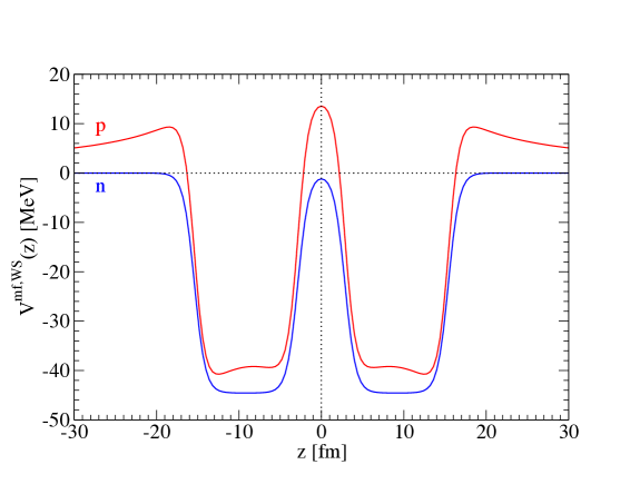
The parameter for the scission point is under discussion, a recent estimate Panebianco gives the range 4 - 6.5 fm and a proposed value of 5.7 fm. The distance between the fragment center of mass points is fm. The mean-field (MF) potentials for neutrons and protons along the symmetry line is shown in Fig 1. The values at the scission point are MeV, MeV. Larger estimates of the scission parameter are reported for ternary fission with larger clusters such as 50Ca Dubna which will not be discussed here.
It is possible to estimate the neutron density at the scission point and to understand whether the density values derived from the Pauli blocking estimates are reasonable. For an exploratory calculation, we use the parametrization of neutron/proton densities in nuclei
| (12) |
with fm, fm, and diffusivities fm, fm Seif . The neutron density at distance fm from the surface is fm-3 for each Cd nucleus so that the value of the neutron density in the neck region is about fm-3. The proton density at this distance is estimated as fm-3. If the distance for scission is larger, fm, the corresponding densities are smaller, fm fm-3.
At this point we emphasize that the treatment of the full Hamiltonian including the external mean-field potential leads to the result that the cluster distributions, including the formation of light nuclei, happens at scales of the rms radii which are of the order 1 - 3 fm. The center-of-mass (c.m.) motion of the cluster is determined by the external potential, whereas the intrinsic properties are determined locally. Intrinsic energy, but also excitations of nuclei and their distribution, are determined by the local properties. The wave function of the c.m. motion is also extended but may be approximated by a quasi-classical approximation. This is not possible for the protons and neutrons which are described by extended states. We cannot treat them like plane waves describing free particles but have to use, e.g., quasiparticle states in the mean-field potential known from HFB calculations.
As a consequence, single-particle modifications of the in-medium few-particle Schrödinger equation like the Hartree-Fock self-energy or the Pauli blocking should be expressed in terms of the quasiparticle wave function and the occupation numbers of these quasiparticle states. It is possible to introduce Wigner functions and to perform a local approximation, but it has to be noted that Pauli blocking and exchange interaction are nonlocal.
For the yields we conclude that all bound states of the light isotopes may be described approximatively by local parameters, in particular the local density approximation with the mean field at the scission point . The corresponding relevant distribution evolves to the final yields and unstable states feed the corresponding stable nuclei seen in the experiment. The distribution of neutrons and protons is not described by a local density approximation but by quasiparticle states obtained from the HFB calculation or other approaches to solve the in-medium Schrödinger equation for a nucleon moving in an external, mean-field potential. For the relevant distribution, the neck densities at the scission point appear as new parameters. The partial densities are not described by the Lagrange parameter as in a local density distribution, but need the solution of the Schrödinger equation with an position dependent external potential. The relevant distribution of quasiparticle states evolve also to the final distribution which is not described here, but have been discussed extensively in the literature (e.g., Boltzmann equations). At the moment, we consider as additional parameters characterizing the distribution of clusters.
VI Conclusions: Relation to thermodynamics
The ternary fission, considered in this work, is a nonequilibrium process. A fundamental approach, for instance the method of the nonequilibrium statistical operator NSO , is required for a systematic treatment. An indispensable requisite is the introduction of the relevant statistical operator reflecting the informations we have about the evolving system. In heavy-ion collisions the hot and dense nuclear matter evolves like a fireball, described by local thermodynamic equilibrium. In the case of spontaneous fission, the concept of a fireball is hard to accept if one assumes that the nucleus before fission is described as a pure quantum state. The freeze-out concept is very successful in describing the formation of clusters and the measured yields, but appears presently as a semi-empirical approach which requires more sophisticated reasoning within a fundamental nonequilibrium approach. We use here a information-theoretical approach which does not require the concept of equilibrium.
We have introduced Lagrange parameters to characterize the state of the system, in particular the distribution function for the different components of nuclear matter. Only in thermodynamic equilibrium are these parameters equivalent to the thermodynamic quantities . This is not valid in the fission process considered here. We have a nonequilibrium situation. However, the Lagrange parameter may be considered as the nonequilibrium generalization of these thermodynamic parameters. For instance, the large difference MeV may be compared with the difference 12.4 MeV of the mean-field potentials shown in Fig. 1 at .
The neck region of the fission process is not homogeneous but exhibits strong gradients in the density distribution, the nuclear mean-field potential and the Coulomb potential. This has to be taken into account if statistical models are used to explain the observed yields. In our approach, the construction of the relevant statistical operator has to be improved considering the full Hamiltonian, which contains the position dependent external potential. A mean-field (Hartree-Fock) calculation can provide us with more realistic single-particle orbitals. A local-density approximation where in equilibrium is interpreted as chemical potential to calculate the neutron/proton density within the ideal Fermi gas model is not valid. In contrast to the cluster states which are localized in the range of few fm, the single-nucleon states are extended and have to be calculated for the mean-field potential as function of the position .
Within this work, we have discussed the information-theoretical approach which leads, in the simplest approximation, to a Boltzmann-like distribution. We improved the treatment of the Hamiltonian of the nucleon system taking the formation of excited, unstable states into account, as well as their decay. In addition, we considered correlations in the continuum and in-medium effects. This way we put forward a quantum statistical treatment of the many-nucleon system. Obviously, the excited states and the resonances should be treated in a manner similar to the stable bound states observed in the final distribution. The inclusion of correlations in the continuum has to be considered, for instance, using the scattering phase shifts as shown by the Beth-Uhlenbeck formula. This improves the treatment of very short-living excitations, but such broad resonances cannot be treated like stable, well-defined bound states as done in a simple nuclear statistical equilibrium calculation.
Of particular importance are in-medium modifications which lead to a modification of the quasiparticle energy and possibly the dissolution of bound states (Mott effect). This is of special significance for the weakly bound, neutron-rich exotic nuclei which are strongly influenced by the medium. They may be used as a sonde to probe the environment. The strong reduction of the yield of the exotic nuclei, observed in many ternary fission experiments, may be explained as a density effect. It gives information about the state of the nucleon system at the time instant where the chemical composition freezes out.
Further considerations such as the formation of heavier nuclei like droplet condensation Sarah have to be included, treating nucleation as a nonequilibrium process.
Future work, in particular the treatment of the external mean-field potential, may give a more detailed description of the nonequilibrium properties and the evolution of cluster distribution in ternary fission processes.
Acknowledgment: This work was supported by the German Research Foundation (DFG), Grant # RO905/38-1, the United States Department of Energy under Grant # DE-FG03-93ER40773, the FCT (Portugal) Projects No. UID/FIS/04564/2019 and UID/FIS/04564/2020, and POCI-01-0145-FEDER-029912, and by PHAROS COST Action CA16214. H.P. acknowledges the grant CEECIND/03092/2017 (FCT, Portugal).
Appendix A Virial expansion
Instead of considering unbound systems (resonances) as bound states, we can calculate their contribution to the density (continuum correlation) according to the Beth-Uhlenbeck formula. In particular, for 2H, deuteron channel, we have (c.f. BU ; HS )
| (13) |
(sum of all phase shifts in c.m. system). The reduction factor follows as
| (14) |
Using the values given in HS we find , see also Tab. 2. The effective binding energy follows as
| (15) |
Using the scattering data, the values for (full) are given in Ref. HS ,
| (16) |
The effective binding energy follows as
| (17) |
and the reduction factor
| (18) |
Values are shown in Tabs. 2, 3. The superscripts denotes scattering phase shifts taken from the scattering length and the effective range. The tildes values are calculated with the quasiparticle correction, see R20 .
| HS | |||||||
|---|---|---|---|---|---|---|---|
| 1 | 19.4 | -2.2132 | 0.9883 | -2.1953 | 0.970737 | -2.2089 | 0.984028 |
| 2 | 6.10 | -2.1125 | 0.94530 | -1.98559 | 0.887183 | -2.05406 | 0.918079 |
| 3 | 4.01 | -1.9103 | 0.9004 | -1.61018 | 0.814696 | -1.72622 | 0.846825 |
| 4 | 3.19 | -1.6319 | 0.8622 | -1.11119 | 0.756954 | -1.24862 | 0.783414 |
| 5 | 2.74 | -1.2796 | 0.8277 | -0.508454 | 0.709419 | -0.640388 | 0.728387 |
| 6 | 2.46 | -0.8887 | 0.8003 | 0.189081 | 0.668749 | 0.0851844 | 0.68043 |
| 7 | 2.26 | -0.4433 | 0.7753 | 0.976248 | 0.632977 | 0.918021 | 0.638264 |
| 8 | 2.11 | 0.0428 | 0.7532 | 1.84889 | 0.600954 | 1.84983 | 0.600883 |
| 9 | 2.00 | 0.5300 | 0.7363 | 2.80304 | 0.571969 | 2.87347 | 0.56751 |
| 10 | 1.91 | 1.0493 | 0.7208 | 3.83476 | 0.545542 | 3.98262 | 0.537535 |
| HS | ||||||
|---|---|---|---|---|---|---|
| 1 | 0.288 | 1.11277 | 1.05942 | 0.346657 | 1.5096 | 0.220999 |
| 2 | 0.303 | 2.16202 | 2.12001 | 0.346454 | 3.0388 | 0.218843 |
| 3 | 0.306 | 3.22432 | 3.23552 | 0.340103 | 4.69126 | 0.209349 |
| 4 | 0.307 | 4.29082 | 4.41082 | 0.331972 | 6.45687 | 0.199046 |
| 5 | 0.308 | 5.3532 | 5.65598 | 0.322647 | 8.33014 | 0.188996 |
| 6 | 0.308 | 6.3532 | 6.97922 | 0.312484 | 10.3071 | 0.179451 |
| 7 | 0.308 | 7.3532 | 8.38453 | 0.30186 | 12.3835 | 0.170492 |
| 8 | 0.309 | 8.54864 | 9.87243 | 0.29111 | 14.5542 | 0.162142 |
| 9 | 0.310 | 9.59871 | 11.4413 | 0.280479 | 16.8142 | 0.154394 |
| 10 | 0.311 | 10.6447 | 13.0883 | 0.270136 | 19.1583 | 0.14722 |
For 5He we consider
| (19) |
(c.m. system) also considered in HS . The reduction factor is
| (20) |
(the degeneracy factor 1/4 follows from the degeneracy factor in the phase shifts). This is the factor to multiply the NSE ground state contribution. Using the values given in HS we find .
For 8Be we consider
| (21) |
(c.m. system) also considered in HS . The reduction factor is
| (22) |
Using the values given in HS we find .
Calculations based on a separable potential approach have been performed in R20 . Using the expressions given there, the reduction factor for 4H is 0.0654. Considering only the channel, the reduction factor for 5He is 0.70716.
The calculation of the contribution of the continuum is more complex for the remaining isotopes. Calculations with separable potentials are possible, but the potential parameters must be fitted to scattering data. We assume that the situation with 7He and 9He is comparable to 5He and take a similat reduction factor. Because these isotopes give only small contributions, a rough estimate is sufficient.
We have also to estimate the contribution of scattering states for isotopes with stable (with respect to strong interaction) ground states, as familiar from the virial expansion. This is known for 2H where we can use the result for the virial expansion given above. For 4He, but also for 3H, 3He, the scattering state contributions are irrelevant because the continuum threshold () is high. For 6He, 8He, where we have also a considerable reduction , we expect a significant contribution from continuum correlations. We consider
| (23) |
with scattering phase shifts as function of the energy in the c.m. system. We can adapt phase shifts from other cases such as or scattering, or perform calculations with a separable potential (e.g. 6He, with fm-1 as for 5He, but instead of 670 MeV fm3 to reproduce the bound state energy) to estimate this contribution. The phase shifts are only weakly decreasing in the low-energy region MeV of relevance, we obtain
References
- (1) C. Wagemans, The Nuclear Fission Process (CRC Press, Boca Raton, 1991).
- (2) J. Mills, Fission Product Yield Evaluation, thesis work, Univ. of Birmingham, 1995.
- (3) IAEA-TECDOC-1168 ISSN 1011 4289 IAEA, Vienna, (2000).
- (4) U. Koester et al.. Nucl. Phys. A 652, 371 (1999).
- (5) U. Koester et al.. Proceedings from the Pont d’Oye IV Conference, October 6-8, 1999, Habay-la-Neuve, Belgium.
- (6) U. Koester, Ausbeuten und Spektroskopie radioaktiver Isotope bei LOHENGRIN und ISOLDE, thesis work, Technische Universität München, 2000.
- (7) S. Wuenschel et al., Phys. Rev. C 90, 011601 (2014).
- (8) Zagrebaev et al., Phys. Rev. C 81, 044608 (2010).
- (9) Artemenkov et al., arXiv:1902.04407 (2019).
-
(10)
P. Holmvall,
Experimental and theoretical refutation of Collinear Cluster
Tri-partition, thesis work, Chalmers Univ. Technology,
Gothenburg, 2014.
P. Holmvall et al., Phys. Rev. C 95, 014602 (2017). - (11) T. V. Chuvilskaya and Yu. M. Tchuvil’sky, Phys. Rev. C 99, 024301 (2019).
- (12) Yu. N. Kopatch, M. Mutterer, D. Schwalm, P. Thirolf, and F. Gönnenwein, Phys. Rev. C 65, 044614 (2002).
- (13) G. V. Val’skii, Yad. Fiz. 67, 1288 (2004) [Sov. J. Nucl. Phys. 67, 1264 (2004)].
- (14) D. N. Zubarev et al., Statistical Mechanics of Nonequilibrium Processes, Vol. I and II (Akademie-Verlag Berlin, 1996/1967).
- (15) U. Koester, Ausbeuten und Spektroskopie radioaktiver Isotope bei LOHENGRIN und ISOLDE, thesis work, Technische Universität München, 2000: Tab. A.5.13.
- (16) G.M. Raisbeck and T.D. Thomas,Phys. Rev. 172, 1272 (1968).
- (17) J.F. Wild et al., Phys. Rev. C 32, 488 (1985).
-
(18)
Wollersheim Cf
https://web-docs.gsi.de/ wolle/FISSION/ternary/node2.html - (19) S.L. Whetstone and T.D. Thomas, Phys. Rev. 154, 1174 (1967).
- (20) M. Mutterer et al., Phys. Rev. C 78, 064616 (2008).
- (21) A. Chietera et al., Eur. Phys. J. A 54, 98 (2018).
- (22) P. Jesinger et al., Eur. Phys. J. A 24, 379 (2005).
- (23) Z. Dlouhy, J. Svanda, R. Bayer and I. Wilhelm, in R. Neugart and A. Wöhr, eds.,6th Int. Conf. on Nuclei far from Stability & 9th Int. Conf. on Atomic Masses and Fund. Const., Bernkastel-Kues, Inst. Phys. Conf. Ser. No. 132, IOP, Bristol (1992), pp. 481 483.
- (24) A.S. Vorobyev, O.A. Shcherbakov, A.M. Gagarski, G.A. Petrov and G.V. Val ski, J. Expt. and Theor. Phys. and Theoretical Physics, 125, 619 (2017).
- (25) L. Stuttgé, A. Chietera, F. Gönnenwein, Yu. Kopatch, M. Mutterer , A. Gagarski , I. Guseva , E. Chernysheva , F.-J. Hambsch , F. Hanappe, Z. Mezentseva, and S. Telezhnikov, EPJ Web of Conferences 193, 03001 (2018).
- (26) A. B. Hansell, A new measurement of the neutron multiplicity emitted in 252Cf spontaneous fission, thesis work, Temple University, Philadelphia, 2020.
- (27) Data tables of nuclei Nudat 2: https://www.nudc.bnl.gov/nudat2/
- (28) S. Albergo et al., Nuovo Cimento A 89, 1 (1985).
- (29) G. Röpke, Phys. Rev. C 101, 064310 (2020).
- (30) E. Beth and G. E. Uhlenbeck, Physica 4, 915 (1937).
- (31) C. J. Horowitz and A. Schwenk, Nucl. Phys. A 776, 55 (2006).
- (32) O. Ivanytskyi et al., Eur. Ohys. J. A 55,184: (2019).
- (33) J.-F. Lemaitre et al., Phys. Rev. C 99, 034612 (2019).
- (34) C. Karthika and M. Balasubramaniam, Eur. Phys. J. A 55, 59 (2019).
- (35) N. Carjan and M. Rizea, Int. J. Mod. Phys. E 28, 1950103 (2019)..
- (36) A. Bulgac et al., Phys. Rev. C 100, 034615 (2019).
- (37) G. F. Bertsch et al., Phys. Rev. C 100, 024607; 044606 (2019).
-
(38)
S. Yang et al., Phys. Rev. C 101, 024316 (2020);
G. Röpke et al., Phys. Rev. C 90, 034304 (2014). - (39) N. Schwierz, I. Wiedenhover, and A. Volya, arxiv:0709.3525
- (40) S. Panebianco et al., Phys. Rev. C 86, 064601 (2012).
-
(41)
A. K. Nasirov et al., Eur. Phys. J. A 52, 135 (2016);
Yu. V. Pyatkov et al., Phys. Rev. C 96, 064606 (2017). - (42) W. M. Seif and H. Mansour, Int. J. Mod. Phys. E. 24, 1550083 (2015).