A fully coupled numerical model of thermo-hydro-mechanical processes and fracture contact mechanics in porous media

Abstract

Various phenomena in the subsurface are characterised by the interplay between deforming structures such as fractures and coupled thermal, hydraulic and mechanical processes. Simulation of subsurface dynamics can provide valuable phenomenological understanding, but requires models which faithfully represent the dynamics involved; these models therefore are themselves highly complex.

This paper presents a mixed-dimensional thermo-hydro-mechanical model designed to capture the process–structure interplay using a discrete–fracture–matrix framework. It incorporates tightly coupled thermo–hydro–mechanical processes based on balance laws for momentum, mass and energy in subdomains representing the matrix and the lower-dimensional fractures and fracture intersections. The deformation of explicitly represented fractures is modelled by contact mechanics relations and a Coulomb friction law, with a novel formulation consistently integrating fracture dilation in the governing equations.

The model is discretised using multi-point finite volumes for the balance equations and a semismooth Newton scheme for the contact conditions and is implemented in the open-source fracture simulation toolbox PorePy. Finally, simulation studies demonstrate the model’s convergence, investigate process–structure coupling effects, explore different fracture dilation models and show an application of the model to stimulation and long-term cooling of a three-dimensional geothermal reservoir.

1 Introduction

Fluid injection operations into the subsurface are common in e.g. geothermal energy and petroleum production, wastewater disposal, CO₂ storage and groundwater management. Injection can severely alter subsurface hydraulic, mechanical, thermal and chemical conditions. These coupled processes are strongly affected by preexisting fractures, which represent extreme heterogeneities and discontinuities in the formation. The processes may in turn cause deformation of the fractures, giving rise to dynamic and highly complex process–structure interactions.

In some subsurface engineering operations, fracture deformation is deliberately induced, e.g. to enhance permeability through hydraulic stimulation, in which fluid is injected at elevated pressure to overcome a fracture’s frictional resistance to slip [1, 2, 3]. There may also be interest in preventing deformation of fractures to, for example, avoid induced seismicity of unacceptable magnitude in disposal of wastewater [4, 5, 6, 7] or during hydraulic stimulation of fractured geothermal reservoirs [8, 9, 10].

As data related to subsurface dynamics are limited, physics-based modelling can complement data analysis in understanding governing mechanisms for fracture deformation. This requires numerical simulation tools that can capture the governing structure of the fractured formation and relevant coupled processes as well as process–structure interactions, which necessitates explicit representation of both the matrix and dominant fractures in the model. Typically, major fractures or faults are represented explicitly while the rest of the domain is represented as a matrix continuum, possibly integrating effects of finer-scale fractures.

In a spatial grid, there are two alternatives for representing such a discrete–fracture–matrix (DFM) model: Resolving the width of the fractures in the grid in an equi-dimensional model imposes severe restrictions put on the spatial discretisation of the domain due to the high aspect ratio of the fractures, thereby limiting the number of fractures that can be included in the model. A geometrically simpler alternative, which was introduced for flow models, is a co-dimension one model, where fractures are represented as objects of one dimension lower than the surrounding domain [11, 12, 13, 14]. In contrast to simulation models for coupled flow and mechanics that treat faults as equidimensional zones of different rheology resolved in the grid [15, 16, 17], the co-dimension DFM model facilitates modelling of fracture slip and dilation [18, 19] and can be combined with full mechanical fracture opening [20, 21]. A conceptually simpler alternative to co-dimension one DFM models is to incorporate only the dynamics in the fracture network and either disregard the dynamics in the matrix altogether or approximate them using semi-analytical methods. These approaches are based on Discrete-Fracture-Network (DFN) representations [22, 23] and will be referred to as DFN methods.

Driven by the need to improve the result of injection operations and avoid unacceptable environmental impacts, intense focus has been placed on physics-based modelling. Early works by Willis-Richards et al. [24], Rahman et al. [25], Kohl and Mégel [26] and Bruel [27] developed DFN-type models considering only deformation and flow in the fractures and using a Coulomb friction law to model fracture slip due to changes in effective stress as a consequence of local change in fluid pressure. Later, Baisch et al. [28] improved on this type of model by including redistribution of shear stress along the fracture as a consequence of slip through a block-spring model. McClure and Horne [29] further developed the modelling of mechanical interaction between fractures with the boundary integral equation method and introduced a rate-and-state friction model. This type of method has been combined with fracture propagation [30, 31]. As only the fracture is discretised when using the boundary integral equation method, models based on this approach can be classified as DFN-type models. Common to all of these approaches is use of semi-analytical approaches and sequential coupling of physical processes.

The last decade has seen developments in the inclusion of dynamics in the matrix as well as improved models and numerical solution schemes for coupling of different dynamics. Building on previously developed DFN-type models, McClure and Horne [29] and McClure [32] introduced a semi-analytical leakoff term to mimic fracture–matrix flow. Norbeck et al. [30] expanded on previous models developed by McClure and Horne [29] and accounted for the interaction between fracture and matrix flow through an embedded discrete fracture model, where flow in the fracture and in the matrix are discretised on non-conforming grids and connected through transfer terms. Hydro-mechanical simulation tools based on co-dimension one DFM models combined with Coulomb friction laws for fracture slip have also been introduced [19, 33, 34, 35, 36, 37, 38], motivated by applications related to CO₂-storage [35], oil and gas production [36, 37] and hydraulic stimulation of fractured geothermal reservoirs [38, 19]. In these tools, the contact mechanics conditions are typically handled through Lagrange-multipliers [35, 34, 33] or penalty methods [36]; see e.g. Wriggers and Zavarise [39].

More recently, thermal effects have been taken into account in deformation of fractured porous media. Based on a DFN-type model, where the boundary integral equation method was used so that only the fracture is discretised, Ghassemi and Zhou [40] included thermo-poroelastic effects in the matrix. Based on a DFM conceptual model, Pandey et al. [41] and Salimzadeh et al. [42] have presented models with linear thermo-poroelasticity for the matrix combined with flow, heat transfer and deformation of a single fracture. However, none of these works included modelling of fracture slip or shear dilation when fracture surfaces are in contact. Gallyamov et al. [21] consider a conceptually similar model which includes multiphase flow and a fracture-contact-mechanics model combined with opening and propagation of fractures, and present simulation studies with a large number of fractures. Their work considers the impact of the contact traction on the hydraulic aperture of closed fractures. In contrast to the majority of previously mentioned works, where simplifications that impact the solution are made in the solution of the coupled system, they solve the equations fully coupled, i.e. the flow, energy and mechanics equations are solved simultaneously building on the work by Garipov et al. [36].

Recent work by Garipov and Hui [43] combines several previous developments. Their work is based on a DFM model and considers a fully coupled thermo-poroelastic model for the matrix, flow and heat transfer in the fractures and contact mechanics for fractures based on a Coulomb friction law. Energy and mass conservation are discretised by a finite volume method, while momentum is discretised by a Galerkin finite element method. This work also presents robust treatment of couplings in the model. However, while the work accounts for permeability enhancement due to full opening of fractures as well as shear dilation, stress response due to dilation as a consequence of slip is not included in the model.

This paper presents a mathematical model based on a mixed-dimensional DFM representation of coupled thermo-hydro-mechanical (THM) processes in a porous rock containing deforming fractures with an accompanying discretisation and numerical solution approach. The model fully couples fluid flow and transport in both matrix and fractures, linear thermo-poromechanics in the matrix and nonlinear fracture deformation. Fracture deformation is based on traction balance, nonpenetration and a Coulomb type friction law, and allows for shear slip and dilation as well as complete fracture opening. To the authors’ knowledge, this is the first model that consistently and fully coupled represents stress redistribution due to slip-induced dilation of fractures. As demonstrated by the numerical results, the effect of this coupling can be significant.

Based on the modelling of fractures as lower-dimensional surfaces, the domain is decomposed into subdomains of different dimensions corresponding to matrix, fractures and intersections. Model equations, sets of variables and parameters are defined on each subdomain and the interfaces between them. The resulting mixed-dimensional model [44] facilitates systematic modelling on the decomposed structure while incorporating interaction between processes both within and between subdomains. The governing balance equations in each subdomain are discretised based on multi-point finite volume methods preserving local conservation, using the same spatial grid for discretisation of all processes. The contact conditions are formulated in terms of contact tractions at the interfaces between fractures and matrix blocks, similar to approaches based on Lagrange-multipliers [39]. The nonlinear fracture deformation equations are discretised using a semismooth Newton scheme formulated as an active set method. The model and its implementation extend the work presented by Berge et al. [34], who consider the poromechanical problem without flow in the fractures, shear dilation and thermal effects.

The model is presented in Section 2, and its discretisation is described in Section 3. In both sections, particular emphasis is placed on fracture deformation as well as its impact on the balance equations for the fractures and the back-coupling to the higher-dimensional momentum balance. Three examples are presented in Section 4: The first investigates governing mechanisms and coupling effects and verifies the model and its implementation in a convergence study. In the second, three different models for fracture dilation are compared. In the last example, the model is applied to a three-dimensional hydraulic stimulation and long-term cooling scenario for geothermal energy extraction. Finally, Section 5 provides some concluding remarks.

2 Mixed-dimensional governing equations

This section describes the model for THM processes in a porous medium with contact mechanics at the fractures. It relies on a DFM model in which the matrix, the fractures and fracture intersections are explicitly represented by individual subdomains. To avoid resolving the small geometric distances introduced to the fracture network geometry by the high aspect ratio of the fractures, the dimensions of the fracture and intersection subdomains are reduced. The subdomains are collected in a hierarchical structure and connected by interfaces to yield the full mixed-dimensional model.

Decomposition into subdomains facilitates tailored modelling of processes in distinct subdomains, while interactions between subdomains take place on the interfaces. Specifically, separate sets of variables, equations and parameters are defined on each subdomain and interface. This procures the flexibility needed to model the highly complex system arising from the coupled THM system posed in both matrix and fractures.

The model consists of balance equations for momentum, mass and energy and relations governing the fracture deformation posed on the subdomains. These are supplemented by constitutive laws and equations for coupling over the interfaces. The equations are formulated in terms of the primary variables displacement, pressure, temperature and contact traction on the fractures.

The governing equations for THM-processes in a mono-dimensional porous medium are introduced succinctly in Section 2.1, followed by a more elaborate presentation of the lower-dimensional scalar equations for deforming fractures and intersections emphasising the effect of volume change in Section 2.2. Section 2.3 describes the model for fracture deformation and its relation to volume change.

2.1 Matrix thermo-poromechanics

We first consider the governing equations in the matrix domain consisting of a solid and a fluid phase. For the remainder of this subsection, let $\Omega$ denote the matrix domain, $\bm{n}$ the outer normal vector on the boundary $\partial\Omega$ and $d\bm{x}=\bm{n}dx$. Neglecting inertia, the momentum balance equation reads

$$\begin{aligned} \int_{\partial\Omega}\sigma\cdot d\bm{x}=\int_{\Omega}\bm{q_{\bm{u}}}dx\end{aligned}$$ (1)

with $\bm{q_{\bm{u}}}$ denoting body forces and the thermo-poroelastic stress tensor for infinitesimal deformation modelled as linearly elastic obeying an extended Hooke’s law

$$\begin{aligned} \sigma-\sigma_{0}=\frac{\mathbf{D}}{2}:(\nabla\bm{u}+\nabla\bm{u}^{T})-\alpha\left(p-p_{0}\right)\mathbf{I}-\beta_{s}K_{s}\left(T-T_{0}\right)\mathbf{I}.\end{aligned}$$ (2)

Here, $\mathbf{D}$ denotes the stiffness tensor, $\alpha$ the Biot coefficient, $\beta_{s}$ the volumetric thermal expansion and $K_{s}$ the bulk modulus of the solid, while $\bm{u}$, $p$, and $\mathbf{I}$ are displacement, pressure and identity matrix. The subscript 0 indicates the reference state of a variable. The assumption of local thermal equilibrium between fluid and solid leads to a single temperature unknown $T$ and to the definition of effective coefficients, which are computed as weighted sums [45]:

$$\begin{aligned} (\cdot)_{e}=\phi(\cdot)_{s}+\left(1-\phi\right)(\cdot)_{f}.\end{aligned}$$ (3)

Subscripts $s$ and $f$ indicate that all quantities in the parentheses are for the solid and fluid, respectively. Herein, the relations $\frac{\mathbf{D}}{2}(\nabla\bm{u}+\nabla\bm{u}^{T})=\mu(\nabla\bm{u}+\nabla\bm{u}^{T})+K_{s}\text{tr}({\nabla\bm{u}})\mathbf{I}$ and $\bm{q_{\bm{u}}}=\rho_{s}\bm{g}$ are used, with $\mu$ denoting the shear modulus, $\text{tr}({\cdot})$ the trace of a tensor, $\rho_{s}$ the solid density and $\bm{g}$ the gravitational acceleration vector.

We assume the density of the slightly compressible fluid to follow

$$\begin{aligned} \rho_{f}=\rho_{0}\exp\left[\frac{1}{K_{f}}(p-p_{0})-\beta_{f}(T-T_{0})\right],\end{aligned}$$ (4)

with $\beta_{f}$ and $K_{f}$ denoting fluid thermal expansion coefficient and bulk modulus, which is the inverse of the compressibility. Balance of mass reads [46]

$$\begin{aligned} \int_{\Omega}\left(\frac{\phi}{K_{f}}+\frac{\alpha-\phi}{K_{s}}\right)\frac{\partial p}{\partial\textit{t}}+\alpha\frac{\partial(\nabla\cdot\bm{u})}{\partial\textit{t}}-\beta_{e}\frac{\partial T}{\partial\textit{t}}dx+\int_{\partial\Omega}\bm{v}\cdot d\bm{x}=\int_{\Omega}q_{p}dx,\end{aligned}$$ (5)

with porosity $\phi$ and effective thermal expansion $\beta_{e}$. Fluid flux relative to the solid is denoted by $\bm{v}$ and volume sources and sinks by $q_{p}$. With $\mathcal{K}$ denoting the permeability and $\eta$ the viscosity, the flux is modelled according to Darcy’s law:

$$\begin{aligned} \bm{v}=-\frac{\mathcal{K}}{\eta}(\nabla p-\rho\bm{g}).\end{aligned}$$ (6)

Neglecting viscous dissipation on an assumption of small velocities [46], the energy balance equation is [47, 48, 46]

$$\begin{aligned} \int_{\Omega}\frac{\partial}{\partial\textit{t}}\left[\phi U_{f}+(1-\phi)U_{s}\right]+\beta_{s}K_{s}T_{0}\frac{\partial(\nabla\cdot\bm{u})}{\partial\textit{t}}dx+\int_{\partial\Omega}(\bm{w}+\bm{q})\cdot d\bm{x}=\int_{\Omega}q_{T}dx.\end{aligned}$$ (7)

Here, the internal energy of the solid is $U_{s}=\rho_{s}c_{s}T$, where $c_{s}$ is the specific heat capacity of the solid. Assuming a simplified low-enthalpy description of the fluid, we approximate the fluid internal energy as $U_{f}=\rho_{f}h_{f}$, where the fluid enthalpy is approximated as $h_{f}=c_{f}T$ and $c_{f}$ is the specific heat capacity of the fluid. The thermoelastic dissipation term involving the displacement represents the effect of the solid elastic deformation on the temperature distribution. The total heat flux is the sum of the advective flux

$$\begin{aligned} \bm{w}=\rho_{f}c_{f}T\bm{v}\end{aligned}$$ (8)

and the diffusive Fourier flux

$$\begin{aligned} \bm{q}=-\kappa_{e}\nabla T.\end{aligned}$$ (9)

In the computation of the effective heat conductivity $\kappa_{e}$ by Eq. (3), dispersion due to micro-scale tortuous flow in the porous medium is neglected. The source term is assumed to equal the internal energy of the fluid of the volume source and sink terms, i.e. $q_{T}=\rho_{f}c_{f}Tq_{p}$.

The energy equation can thus be written

$$\begin{aligned} \int_{\Omega}\frac{\partial}{\partial\textit{t}}\Big{[}(\rho c)_{e}T\Big{]}+\beta_{s}K_{s}T_{0}\frac{\partial(\nabla\cdot\bm{u})}{\partial\textit{t}}dx+\int_{\partial\Omega}(\rho_{f}c_{f}T\bm{v}-\kappa_{e}\nabla T)\cdot d\bm{x}=\int_{\Omega}q_{T}dx.\end{aligned}$$ (10)

where $(\rho c)_{e}$ denotes the effective heat capacity of the porous medium and is calculated by Eq. (3). The first term of Eq. (10) can be expanded, giving

$$\begin{aligned} \frac{\partial}{\partial\textit{t}}\Big{[}(\rho c)_{e}T\Big{]}=(\rho c)_{e}\frac{\partial T}{\partial\textit{t}}+T\frac{\partial(\rho c)_{e}}{\partial\textit{t}}=(\rho c)_{e}\frac{\partial T}{\partial\textit{t}}+T\left[\left(\frac{\rho c}{K}\right)_{e}\frac{\partial p}{\partial\textit{t}}-\left(\rho c\beta\right)_{e}\frac{\partial T}{\partial\textit{t}}\right],\end{aligned}$$ (11)

where effective parameters are calculated using Eq. (3).

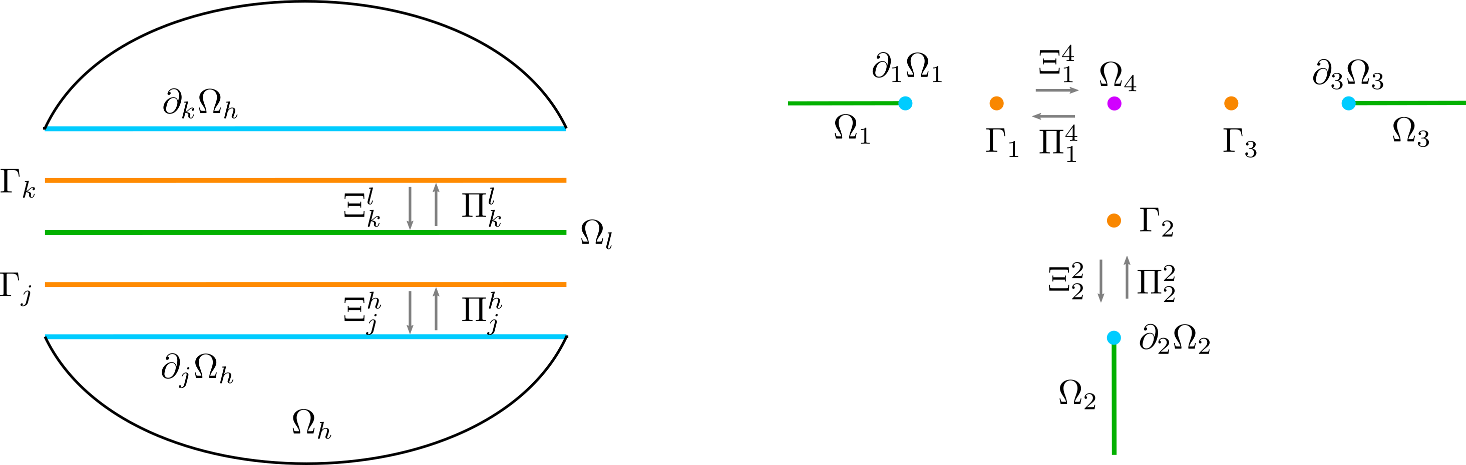
Figure 1: Schematic representation of a throughgoing one-dimensional fracture in a two-dimensional matrix (left) and three fractures meeting at an intersection point (right). All subdomains, internal boundaries and interfaces are indicated, as are select projection operators. $\Omega_{h}$ and $\Omega_{l}$ are separated by the interfaces $\Gamma_{j}$ and $\Gamma_{k}$ corresponding to the internal boundaries $\partial_{j}\Omega_{h}$ and $\partial_{k}\Omega_{h}$. The intersecting fractures are indexed counterclockwise from 1 through 3 and intersect at the point $\Omega_{4}$. The interfaces are numbered so that $\Gamma_{i}$ matches $\partial_{i}\Omega_{i}$. In the model, $\Omega_{l}$, $\Gamma_{j}$, $\Gamma_{k}$, $\partial_{j}\Omega_{h}$ and $\partial_{k}\Omega_{h}$ coincide geometrically, as do all zero-dimensional points in the right figure.

2.2 Lower-dimensional flow and heat transfer

This section derives balance equations for mass and energy for fluid-filled fractures and intersections which may undergo significant relative deformation and volume change, giving rise to an additional term compared to equations for static domains. Along with outlining dimension reduction for the mass and energy equations, the connection between the subdomains of the mixed-dimensional model is presented.

Some notation is needed for a unified description of the mixed-dimensional model of a fractured porous domain of dimension $D=3$ or $D=2$. The domain is split into connected subdomains corresponding to the rock matrix, the co-dimension one fracture planes and co-dimension two fracture intersections. In the case $D=3$, the model also generalises to account for intersections of fracture intersection lines, i.e. zero-dimensional points. A subdomain is denoted by $\Omega_{i}$ and its boundary by $\partial\Omega_{i}$. The subscript $i$ is also used to identify variables defined within $\Omega_{i}$, but suppressed as context allows. Each part $\partial_{j}\Omega_{i}$ of the internal boundary is associated with an interface $\Gamma_{j}$ to an immersed lower-dimensional domain $\Omega_{l}$ (see Fig. 1). All lower- and higher-dimensional interfaces of a subdomain are collected in the sets $\check{S}$ and $\hat{S}$; in particular, the interfaces corresponding to surfaces of fracture $i$ constitute $\hat{S}_{i}$. Where convenient, the higher- and lower-dimensional neighbours of an interface are denoted by $\Omega_{h}$ and $\Omega_{l}$, respectively.

Finally, four types of projection operators are needed to transfer variables between interfaces and the neighbouring higher- and lower-dimensional subdomains. As illustrated in Fig. 1, projection from the interface to the subdomains is performed by $\Xi^{h}_{j}$ and $\Xi^{l}_{j}$, respectively, whereas $\Pi^{h}_{j}$ and $\Pi^{l}_{j}$ project from the part of a subdomain geometrically coinciding with the interface to the interface.

The thickness of a fracture is characterised by the aperture $a$ [$\mathrm{m}$], which will be related to the fracture deformation in Section 2.3. The aperture of an intersection is taken to be the average of the intersecting higher-dimensional neighbours, i.e.

$$a_{l}=\frac{1}{|\hat{S}_{l}|}\sum_{j\in\hat{S}_{l}}\Xi^{l}_{j}\Pi^{h}_{j}a_{h},$$ (12)

where the projection operators transfer the higher-dimensional aperture first to the interface and then to the intersection, see Fig. 1. The specific volume $\mathcal{V}_{i}=a^{D-d}$ accounts for the dimension reduction from the deforming equi-dimensional $\Omega$ to the corresponding spatially fixed $d$-dimensional $\Omega_{i}$. With $\mathcal{V}=1$ for $d=D$, dimension reduction for a scalar quantity $\zeta$ and a vector quantity $\bm{\iota}$ satisfy

$$\begin{aligned} \frac{d}{d\textit{t}}\int_{\Omega}\zeta dx&=\int_{\Omega_{i}}\frac{\partial}{\partial\textit{t}}(\mathcal{V}_{i}\zeta_{i})dx\end{aligned}$$ (13)

and

$$\begin{aligned} \int_{\partial\Omega}\bm{\iota}\cdot d\bm{x}&=\int_{\partial\Omega_{i}}\mathcal{V}_{i}\bm{\iota}_{i}\cdot d\bm{x}-\sum_{j\in\hat{S}_{i}}\Xi^{l}_{j}\bigg{(}\Pi^{h}_{j}\mathcal{V}_{h}\int_{\Gamma_{j}}\iota_{j}dx\bigg{)},\end{aligned}$$ (14)

respectively. Here, $\bm{\iota}_{i}$ denotes the tangential $d$-dimensional flux, while the interface flux into the domain $\iota_{j}$ satisfies $\Xi^{h}_{j}\iota_{j}=\bm{\iota}_{h}\cdot\bm{n}_{h}$ on $\partial_{j}\Omega_{h}$, with $\bm{n}_{h}$ denoting the outwards normal vector of $\Omega_{h}$. The weighting with $\mathcal{V}_{h}$ ensures that the interface flux matches the dimension of fluxes of the higher-dimensional neighbour, which are scaled by specific volumes as seen by the expression for the tangential flux. Note that all differentials in reduced integrals should be interpreted as relative to the domain of integration; i.e. $dx$ is two-dimensional for a fracture with $d=2$. Furthermore, $d\bm{x}=\bm{n}_{i}dx$, where $\bm{n}_{i}$ denotes the outwards normal at $\partial\Omega_{i}$ lying in the tangent plane of $\Omega_{i}$. For $d=1$, the boundary integral equals evaluation of the integrand at the boundary points.

Assuming unitary fracture porosity, the fluid mass balance equation for a deforming equi-dimensional domain $\Omega$ is

$$\begin{aligned} \frac{d}{d\textit{t}}\int_{\Omega}\rho_{f}dx+\int_{\partial\Omega}\rho_{f}\bm{v}\cdot d\bm{x}=\int_{\Omega}\rho_{f}q_{p}dx.\end{aligned}$$ (15)

Averaging in the normal direction for the tangential flux and replacing the normal part of the boundary by $\Gamma_{j}$ according to Eq. (14), the fluid flux becomes

$$\begin{aligned} \int_{\partial\Omega}\bm{v}\cdot d\bm{x}=\int_{\partial\Omega_{i}}\mathcal{V}_{i}\bm{v}_{i}\cdot d\bm{x}-\sum_{j\in\hat{S}_{i}}\Xi^{l}_{j}\bigg{(}\Pi^{h}_{j}\mathcal{V}_{h}\int_{\Gamma_{j}}v_{j}dx\bigg{)}.\end{aligned}$$ (16)

Thus, the interdimensional coupling between $\Omega_{h}$ and $\Omega_{l}$ takes the form of interface fluid fluxes $v_{j}$, which also appear as a Neumann condition for $\Omega_{h}$:

$$\begin{aligned} \bm{v}_{h}\cdot\bm{n}_{h}=\Xi^{h}_{j}v_{j}.\end{aligned}$$ (17)

The interface flux is modelled using a Darcy type law extended from Martin et al. [12] to account for gravity

$$\begin{aligned} v_{j}=-\frac{\mathcal{K}_{j}}{\Pi^{l}_{j}\eta_{l}}\bigg{(}\frac{2}{\Pi^{l}_{j}a_{l}}\left(\Pi^{l}_{j}p_{l}-\Pi^{h}_{j}p_{h}\right)-\Pi^{l}_{j}\rho_{f,l}\bm{g}\cdot\Pi^{h}_{j}\bm{n}_{h}\bigg{)}.\end{aligned}$$ (18)

Both the weighting by $a_{l}$ and $\mathcal{V}_{h}$ and the normal permeability $\mathcal{K}_{j}$ arise through dimension reduction. The remaining terms of Eq. (15) are averaged in the normal direction using Eq. (13), and Eq. (4) is inserted for the fluid density. Collecting terms, dividing by $\rho_{f}$ and assuming Darcy’s law with tangential permeability $\mathcal{K}$ yields the dimensionally reduced mass balance

$$\begin{aligned} &\int_{\Omega_{i}}\mathcal{V}_{i}\left(\frac{1}{K_{f}}\frac{\partial p_{i}}{\partial\textit{t}}-\beta_{f}\frac{\partial T_{i}}{\partial\textit{t}}\right)+\frac{\partial\mathcal{V}_{i}}{\partial\textit{t}}dx-\int_{\partial\Omega_{i}}\mathcal{V}_{i}\frac{\mathcal{K}}{\eta}\left(\nabla p_{i}-\rho_{f}\bm{g}\right)\cdot d\bm{x}\\ &-\sum_{j\in\hat{S}_{i}}\Xi^{i}_{j}\bigg{(}\Pi^{h}_{j}\mathcal{V}_{h}\int_{\Gamma_{j}}v_{j}dx\bigg{)}=\int_{\Omega_{i}}\mathcal{V}_{i}q_{p}dx,\end{aligned}$$ (19)

with the third term accounting for changes in fracture volume.

The dimension reduction is now performed for the energy balance, which for an equi-dimensional domain reads

$$\begin{aligned} \frac{d}{d\textit{t}}\int_{\Omega}\rho_{f}c_{f}Tdx+\int_{\partial\Omega}\left(\bm{w}+\bm{q}\right)\cdot d\bm{x}=\int_{\Omega}q_{T}dx,\end{aligned}$$ (20)

where $\bm{w}$ and $\bm{q}$ are given by Eqs. (8) and (9). Utilising Eq. (14), the dimension reduction of the flux terms is

$$\begin{aligned} \int_{\partial\Omega}\bigg{(}\bm{w}+\bm{q}\bigg{)}\cdot d\bm{x}=\int_{\partial\Omega_{i}}\mathcal{V}_{i}\bigg{(}\bm{w}_{i}+\bm{q}_{i}\bigg{)}\cdot d\bm{x}-\sum_{j\in\hat{S}_{i}}\Xi^{l}_{j}\bigg{(}\Pi^{h}_{j}\mathcal{V}_{h}\int_{\Gamma_{j}}w_{j}+q_{j}dx\bigg{)},\end{aligned}$$ (21)

and the internal boundary conditions on $\partial_{j}\Omega_{h}$ are

$$\begin{aligned} \bm{w}_{h}\cdot\bm{n}_{h}&=\Xi^{h}_{j}w_{j},\\ \bm{q}_{h}\cdot\bm{n}_{h}&=\Xi^{h}_{j}q_{j}.\end{aligned}$$ (22)

The advective interface flux is defined according to the upstream direction of the interface fluid flux:

$$\begin{aligned} w_{j}=\left\{\begin{array}[]{ l l }v_{j}\Pi^{h}_{j}\rho_{f,h}c_{f,h}T_{h}&\text{ if }v_{j}>0\\ v_{j}\Pi^{l}_{j}\rho_{f,l}c_{f,l}T_{l}&\text{ if }v_{j}\leq 0.\end{array}\right.\end{aligned}$$ (23)

The Fourier-type conductive interface flux is

$$\begin{aligned} q_{j}=-\kappa_{j}\frac{2}{\Pi^{l}_{j}a_{l}}(\Pi^{l}_{j}T_{l}-\Pi^{h}_{j}T_{h}),\end{aligned}$$ (24)

with the normal heat conductivity modelled as $\kappa_{j}=\Pi^{l}_{j}\kappa_{f,l}$ since it originates from the dimension reduction of a fluid-filled domain.

The dimension reduction of the remaining terms of Eq. (20) is performed by again invoking Eq. (13), yielding

$$\begin{aligned} \int_{\Omega_{i}}c_{f}\rho_{f}T_{i}\frac{\partial\mathcal{V}_{i}}{\partial\textit{t}}&+\mathcal{V}_{i}\frac{\partial}{\partial\textit{t}}\bigg{(}\rho_{f}c_{f}T_{i}\bigg{)}dx+\int_{\partial\Omega_{i}}\mathcal{V}_{i}\bigg{(}\rho_{f}c_{f}T_{i}\bm{v}_{i}-\kappa_{f}\nabla T_{i}\bigg{)}\cdot d\bm{x}\\ &-\sum_{j\in\hat{S}_{i}}\Xi^{i}_{j}\bigg{(}\Pi^{h}_{j}\mathcal{V}_{h}\int_{\Gamma_{j}}w_{j}+q_{j}dx\bigg{)}=\int_{\Omega_{i}}\mathcal{V}_{i}q_{T}dx,\end{aligned}$$ (25)

where the second term in the first integral is decomposed similarly to Eq. (11), with $\phi=1$ in the calculation of effective coefficients.

2.3 Fracture contact mechanics

The traction balance, nonpenetration condition and friction law posed on a fracture $l$ are formulated in terms of interface displacements and fracture contact traction. The interface displacements on the two surfaces $\Gamma_{j}$ and $\Gamma_{k}$ are $\bm{u}_{j}$ and $\bm{u}_{k}$, and the jump between the two sides is

$$\begin{aligned} [\![\bm{u}_{l}]\!]=\Xi^{l}_{k}\bm{u}_{k}-\Xi^{l}_{j}\bm{u}_{j}.\end{aligned}$$ (26)

Since the fracture deformation depends on traction caused by the contact between the two surfaces, the contribution from $p_{l}$ should be subtracted on the fracture surfaces to yield the traction balance posed on the interfaces:

$$\begin{aligned} \Pi^{l}_{j}\bm{\lambda}_{l}-p_{l}\mathbf{I}\cdot\bm{n}_{l}&=\Pi^{h}_{j}\sigma_{h}\cdot\bm{n}_{h}\quad\quad&\text{on }&\Gamma_{j},\\ \Pi^{l}_{k}\bm{\lambda}_{l}-p_{l}\mathbf{I}\cdot\bm{n}_{l}&=-\Pi^{h}_{k}\sigma_{h}\cdot\bm{n}_{h}\quad\quad&\text{on }&\Gamma_{k}.\end{aligned}$$ (27)

The fracture contact traction $\bm{\lambda}_{l}$ will for notational convenience be referred to as $\bm{\lambda}$ in the following, and is defined according to the normal of the fracture, which is defined to equal $\bm{n}_{h}$ on the $j$ side, i.e. $\bm{n}_{l}=\Xi^{l}_{j}\Pi^{h}_{j}\bm{n}_{h}$. When there is no mechanical contact between the interfaces, $\bm{\lambda}$ is 0, implying that the higher-dimensional thermo-poromechanical tractions projected to the interfaces on the right-hand sides of Eq. (27) are balanced by the fracture pressure.

A vector $\bm{\iota}$ defined on a fracture may be decomposed into the normal and tangential components

$$\iota_{n}=\bm{\iota}\cdot\bm{n}_{l}\text{ and }\bm{\iota}_{\tau}=\bm{\iota}-\iota_{n}\bm{n}_{l}.$$ (28)

With this notation, the nonpenetration condition reads

$$\begin{aligned} [\![\bm{u}]\!]_{n}-g&\geq 0,\\ \lambda_{n}([\![\bm{u}]\!]_{n}-g)&=0,\\ \lambda_{n}&\leq 0,\end{aligned}$$ (29)

with the gap function $g$ defined to equal the distance between the two fracture interfaces when in contact. The Coulomb friction law is

$$\begin{aligned} ||\bm{\lambda}_{\tau}||&\leq-F\lambda_{n},\\ ||\bm{\lambda}_{\tau}||&<-F\lambda_{n}\rightarrow[\![\dot{\bm{u}}]\!]_{\tau}=0,\\ ||\bm{\lambda}_{\tau}||&=-F\lambda_{n}\rightarrow\exists\,\zeta\in\mathbb{R^{+}}:[\![\dot{\bm{u}}]\!]_{\tau}=\zeta\bm{\lambda}_{\tau},\end{aligned}$$ (30)

with $F$ denoting the friction coefficient and $[\![\dot{\bm{u}}]\!]_{\tau}$ denoting the tangential displacement increment. In addition to enforcing the traction balance of Eq. (27) and the conditions of Eqs. (29) and (30), a Dirichlet condition is assigned on $\partial_{j}\Omega_{h}$ so that

$$\Xi^{h}_{j}\bm{u}_{j}=\bm{u}_{h}.$$ (31)

The aperture introduced in Section 2.2 is a function of displacement jump, $a=a\left([\![\bm{u}]\!]\right)$. Due to roughness of the fracture surfaces, tangential displacements may induce dilation [49] as illustrated in Fig. 2. The relationship between the dilation and the magnitude of tangential displacement is assumed to be linear and described by the dilation angle $\psi$ following Rahman et al. [25]. As modelled herein, the dilation is not merely a hydraulic effect impacting e.g. the fracture permeability, but a mechanical effect in the sense that the normal distance between the fracture surfaces increases. As such, the dilation must be coupled back to the normal interface displacements and the matrix deformation through Eq. (31), which is achieved by choosing the gap function

$$g=\tan(\psi)||[\![\bm{u}]\!]_{\tau}||.$$ (32)

The update is reversible; if the tangential displacement is reversed, $g$ takes on its initial value.

Small-scale fracture roughness may provide a volume for the fluid to occupy even when the fractures are in an undeformed state. This leads to the following relation between aperture and displacement:

$$a=a_{0}+[\![\bm{u}]\!]_{n},$$ (33)

where $a_{0}$ denotes the residual aperture in the undeformed state.

In addition to entering the equations as a result of dimension reduction, $a$ governs the tangential permeability of a fracture or intersection line $i$ according to the cubic law [50],

$$\mathcal{K}_{i}=\frac{a_{i}^{2}}{12}\mathbf{I}_{i},$$ (34)

where $\mathbf{I}_{i}$ denotes the identity matrix of the fracture dimension. Equation (34) constitutes a strongly nonlinear coupling, especially as $\mathcal{K}_{i}$ is multiplied by $\mathcal{V}$ in Eq. (19). Finally, the normal permeability of an interface is inherited from the lower-dimensional neighbour:

$$\mathcal{K}_{j}=\Pi^{l}_{j}\mathcal{K}_{l}.$$ (35)

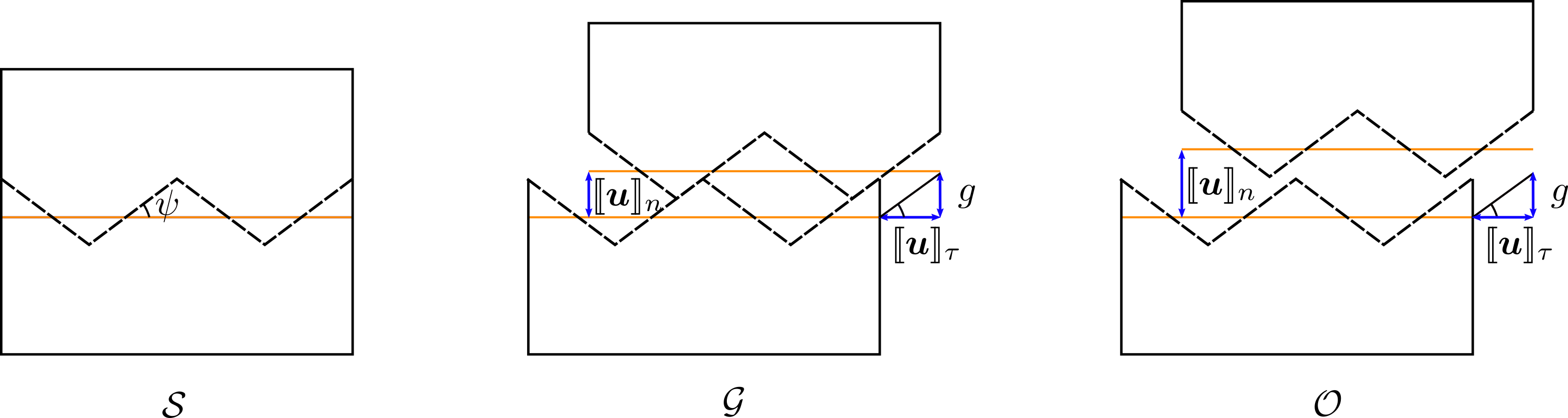
Figure 2: Schematic representation of three fracture configurations: sticking ($\mathcal{S}$), gliding ($\mathcal{G}$) and open ($\mathcal{O}$). In the model, the fracture surfaces are represented as planar interfaces indicated by the orange lines. Idealised fracture roughness is shown by dashed sawtooth lines, with the inclination of the teeth equalling the dilation angle $\psi$, while the magnitude of displacement jumps and $g$ are indicated by arrows. In the first configuration, the fracture is undisplaced and closed with $g=[\![\bm{u}]\!]_{n}=[\![\bm{u}]\!]_{\tau}=0$. In the second configuration, the fracture is still mechanically closed, but tangential displacement has resulted in fracture dilation due to roughness. In the third configuration, there is no mechanical contact across the fracture; that is, the fracture is mechanically open with $[\![\bm{u}]\!]_{n}>g$.

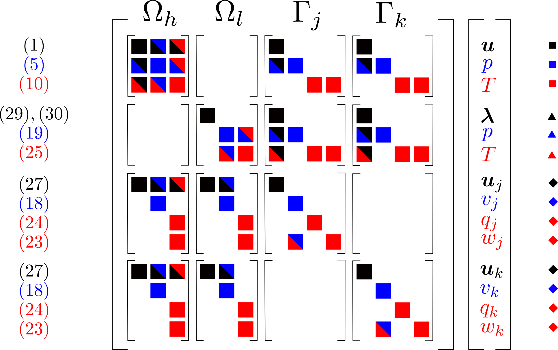
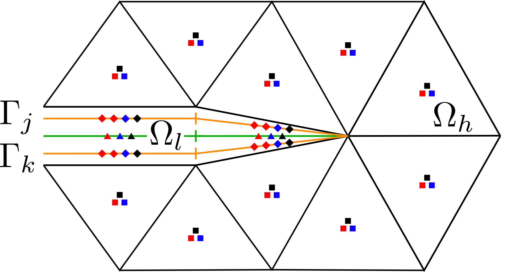
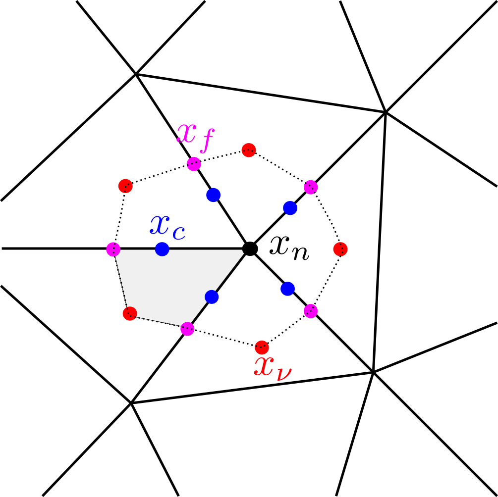
Figure 3: Top: The two-level block structure represents the left-hand side of the linear equation system for a matrix $\Omega_{h}$, a fracture $\Omega_{l}$ and interfaces $\Gamma_{j}$ and $\Gamma_{k}$ with corresponding equation numbers shown to the left. Bottom left: Spatial discretisation and spatial location of degrees of freedom for a domain corresponding to the equation system. Matrix, fracture and interface grids are shown in black, green and orange, respectively, and the corresponding degrees of freedom are shown as squares, triangles and diamonds. Black represents displacement, blue pressure and red temperature; the relation between all markers and unknowns is shown at top right. Bottom right: Subgrid around a node $x_{n}$ of the primary grid, which is shown in solid black lines. The O-shaped interaction region forming the stencil for the local systems is constructed by connecting the surrounding cell centres $x_{\nu}$ and face centres $x_{f}$ as indicated by the dotted lines. Continuity of primary variables is enforced in the points $x_{c}$; the shaded area indicates a subcell.

3 Discretisation

This section describes the discretisation of the model presented in the previous section. The system is discretised in time using implicit Euler and solved monolithically using a direct solver [51]; a more scalable option would be to use iterative methods with block-preconditioners, following ideas in e.g. [52, 53]. The spatial grids are simplicial, and are constructed such that the lower-dimensional cells coincide with higher-dimensional faces; grids are generated by Gmsh [54]. The model is implemented in the open-source fracture simulation toolbox PorePy presented by Keilegavlen et al. [44].

The mixed-dimensional framework gives rise to a two-level block structure as the equations are discretised. The outer level corresponds to the subdomains and interfaces, with entries internal to the subdomains on the diagonal and entries for the interdimensional coupling on the off-diagonals. The inner level corresponds to the primary variables, with coupling effects between different variables on the off-diagonals. The block structure is illustrated in Fig. 3, which will be used in the following description of discretisation of individual terms by referring to the block in row $r$ and column $c$ as $A_{(r,c)}$ with $r$ and $c$ ranging from 1 to 14.

3.1 Matrix thermo-poromechanics

The spatial discretisation of the diffusive terms of the balance equations is achieved using a family of cell-centred finite volume schemes. The approach is based on the multi-point flux approximation (MPFA) [55] defined for diffusive scalar problems and the multi-point stress approximation (MPSA) for vector problems [56] and their combination for THM problems [57, 58]. The scheme is formulated in terms of discrete displacement ($D$ vectors), pressure and temperature unknowns and is locally momentum, mass and energy conservative.

The scheme’s construction is based on a subdivision of the spatial grid as illustrated in Fig. 3, with the gradients of displacement, pressure and temperature defined as piecewise constants on the subdivision. The fluxes of the conserved quantities momentum, mass and energy are discretised via Hooke’s, Darcy’s and Fourier’s law, respectively. Continuity is enforced for traction and mass and energy fluxes over faces of the subgrid and for the primary variables in the continuity points $x_{c}$, leading to one local system for the node of the primary grid. Each local system is partially inverted to express gradients in terms of the cell-centre values in nearby cells. A global system is constructed by collecting for each cell all face fluxes as expressed in terms of the cell-centred primary variables. For details, see Nordbotten and Keilegavlen [58].

The coupling between the three equations is achieved by using the thermo-poroelastic stress for the local traction balances, which directly yields the contributions $A_{(1,2)}$ and $A_{(1,3)}$ representing the scalar variables’ effect on the momentum balance. $A_{(2,1)}$ and $A_{(3,1)}$, which represent the displacement effects on the scalar balances, are constructed by assembly of the discrete divergence based on the local systems for the displacement gradients.

The standard finite volume implicit Euler discretisation is applied to all time derivatives; that is, both the TH coupling blocks $A_{(2,3)}$ and $A_{(3,2)}$ and the accumulation terms of $A_{(2,2)}$ and $A_{(3,3)}$. The advective term of Eq. (10) is discretised using a first-order upwind scheme, i.e. the temperature flux between cells $k$ and $l$ is

$$\begin{aligned} \left(\rho_{f}c_{f}T\bm{v}\right)_{k,l}=\left\{\begin{array}[]{ l l }c_{f}\bm{v}_{k,l}T_{k}\rho_{f,k}&\text{ if }\bm{v}_{k,l}>0\\ c_{f}\bm{v}_{k,l}T_{l}\rho_{f,l}&\text{ if }\bm{v}_{k,l}\leq 0,\end{array}\right.\end{aligned}$$ (36)

with the fluid flux from cell $k$ to cell $l$ $\bm{v}_{k,l}$ and $\rho_{f}$ computed from the solution at the previous iteration.

3.2 Mixed-dimensional flow and heat transfer

All terms of the scalar equations for the lower-dimensional subdomains are discretised using lower-dimensional versions of the corresponding $D$-dimensional discretisations. For the Darcy and Fourier fluxes, this implies that we use the MPFA scheme, while the advective fluxes are again treated by first-order upwinding. The interdimensional coupling relations are discrete analogues to Eqs. (18), (24) and (23). Thus, they involve reconstruction of $p$ and $T$ on $\partial_{j}\Omega_{h}$, which we base on discretisation matrices pertaining to the MPFA discretisations. For the matching grids used herein, the discrete projections are straightforward bijective mappings between faces of $\Omega_{h}$ and cells of $\Gamma_{j}$ ($\Pi^{h}_{j}$ and $\Xi^{h}_{j}$) and between the cells of $\Omega_{l}$ and $\Gamma_{j}$ ($\Pi^{l}_{j}$ and $\Xi^{l}_{j}$).

The nonlinearities arising through the products involving $a$ and $\mathcal{V}$ are solved iteratively within the Newton scheme for fracture deformation described below. Specifically, the time derivatives are computed as additional right hand side terms based on values from the previous iterate and time step. However, the linear volume-change terms in the fractures are coupled fully implicitly to $\bm{u}_{j}$ so that the contribution for each fracture is the jump between the neighbouring higher-dimensional interfaces, as illustrated by the off-diagonal blocks $A_{(5,7)}$, $A_{(5,11)}$, $A_{(6,7)}$ and $A_{(6,11)}$. Densities are computed from the solution at the previous iteration. In some simulations involving strong advection and high temperature gradients, the density dependence in the gravity term of Darcy’s law may lead to oscillatory fluxes between Newton iterations. This may result in convergence problems related to the upstream discretisation of the advective term. In these situations, convergence was achieved by damping the updates of the fluid flux of the advective term.

3.3 Fracture contact mechanics

Fracture deformation discretisation is based on the approach presented by Hüeber et al. [59] and Wohlmuth [60] with the frictional contact problem formulated as a variational inequality. The formulation is expanded to account for the $[\![\bm{u}]\!]_{\tau}$ dependency of $g$. Deformation constraints are reformulated as complementary functions $\mathcal{C}=\mathcal{C}(\mathbb{X})$, with $\mathbb{X}$ being the unknowns. The constraints are imposed by solving $\mathcal{C}=0$ through application of the semismooth Newton method

$$\mathcal{D}(\mathbb{X}^{k})(\delta\mathbb{X}^{k})=-\mathcal{C}(\mathbb{X}^{k}),$$ (37)

where $\delta\mathbb{X}^{k}=\mathbb{X}^{k+1}-\mathbb{X}^{k}$. Correspondingly, the increment of a function $f$ between successive iterations $k$ and $k+1$ is $\delta f(\mathbb{X}^{k})=f(\mathbb{X}^{k+1})-f(\mathbb{X}^{k})$. $\mathcal{D}$ is the generalised Jacobian of $\mathcal{C}$, i.e. the convex hull of the standard Jacobian wherever $\mathcal{C}$ is differentiable.

To facilitate imposition of different constraints based on the deformation states defined in Eqs. (29) and (30), three disjoint sets describing the deformation state as open, sticking or gliding are defined:

$$\begin{aligned} \mathcal{O}&=\left\{b\leq 0\right\},\\ \mathcal{S}&=\left\{||\bm{\lambda}_{\tau}+\tilde{c}[\![\dot{\bm{u}}]\!]_{\tau}||<b\right\},\\ \mathcal{G}&=\left\{||\bm{\lambda}_{\tau}+\tilde{c}[\![\dot{\bm{u}}]\!]_{\tau}||\geq b>0\right\}.\end{aligned}$$ (38)

Here, $\tilde{c}$ denotes a numerical parameter, the friction bound is $b=-F(\lambda_{n}+\tilde{c}\left([\![\bm{u}]\!]_{n}-g\right))$ and $[\![\dot{\bm{u}}]\!]_{\tau}$ denotes the increment from the previous time step. Replacing $[\![\dot{\bm{u}}]\!]_{\tau}$ by $[\![\bm{u}]\!]_{\tau}$ in the above definition yields the cumulative fracture state sets, which are denoted by subscript $c$.

The normal and tangential complementary functions are

$$\begin{aligned} \mathcal{C}_{n}\left([\![\bm{u}]\!]_{n},\lambda_{n}\right)=-\lambda_{n}-\frac{1}{F}\text{max}(0,b)\end{aligned}$$ (39)

and

$$\begin{aligned} \mathcal{C}_{\tau}\left([\![\delta\bm{u}]\!]_{\tau},[\![\bm{u}]\!]_{\tau},\bm{\lambda}{\tau}\right)=\text{max}(b,||\bm{\lambda}_{\tau}+\tilde{c}[\![\bm{u}]\!]_{\tau}||)\left(-\bm{\lambda}_{\tau}\right)+\text{max}(0,b)(\bm{\lambda}_{\tau}+\tilde{c}[\![\dot{\bm{u}}]\!]_{\tau}).\end{aligned}$$ (40)

The corresponding generalised Jacobians are

$$\begin{aligned} \mathcal{D}_{n}\left([\![\bm{u}]\!],\lambda_{n}\right)\left(\delta[\![\bm{u}]\!],\delta\lambda_{n}\right)&=-\delta\lambda_{n}-\chi_{\mathcal{S}\cup\mathcal{G}}\frac{1}{F}\delta b\end{aligned}$$ (41)

and

$$\begin{aligned} \mathcal{D}_{\tau}\left([\![\bm{u}]\!],[\![\dot{\bm{u}}]\!]_{\tau},\bm{\lambda}\right)\left(\delta[\![\bm{u}]\!],\delta[\![\dot{\bm{u}}]\!]_{\tau},\delta\bm{\lambda}\right)=&-\text{max}(b,||\bm{\lambda}_{\tau}+\tilde{c}[\![\dot{\bm{u}}]\!]_{\tau}||)\delta\bm{\lambda}_{\tau}\\ &-\chi_{\mathcal{O}\cup\mathcal{G}}\frac{\bm{\lambda}_{\tau}\left(\bm{\lambda}_{\tau}+\tilde{c}[\![\dot{\bm{u}}]\!]_{\tau}\right)^{T}}{||\bm{\lambda}_{\tau}+\tilde{c}[\![\dot{\bm{u}}]\!]_{\tau}||}\left(\delta\bm{\lambda}_{\tau}+\tilde{c}\delta[\![\dot{\bm{u}}]\!]_{\tau}\right)\\ &+\chi_{\mathcal{S}\cup\mathcal{G}}\,b\left(\delta\bm{\lambda}_{\tau}+\tilde{c}\delta[\![\dot{\bm{u}}]\!]_{\tau}\right)\\ &-\chi_{\mathcal{S}}\,\delta b\bm{\lambda}_{\tau}\\ &+\chi_{\mathcal{S}\cup\mathcal{G}}\,\delta b(\bm{\lambda}_{\tau}+\tilde{c}[\![\dot{\bm{u}}]\!]_{\tau}).\end{aligned}$$ (42)

Here, $\chi_{\star}$ is the characteristic function of a set $\star$ for a fracture cell $\nu$,

$$\chi_{\star}=\left\{\begin{array}[]{ l l }1&\text{ if }\nu\in\star\\ 0&\text{ if }\nu\notin\star,\\ \end{array}\right.$$ (43)

while the increment of the friction bound is

$$\delta b=-F[\delta\lambda_{n}+\tilde{c}\left(\delta[\![\bm{u}]\!]_{n}-g_{\bm{u}}\delta[\![\bm{u}]\!]_{\tau}\right)],$$ (44)

with $g_{\bm{u}}$ denoting the derivative of $g$ with respect to $[\![\bm{u}]\!]$. Hence, sorting each cell according to Eq. (38) and imposing Eq. (37) results in the following constraints:

$$\begin{aligned} \bm{\lambda}^{\nu,k+1}&=\bm{0}&\nu\in\mathcal{O},\\ [\![\bm{u}^{\nu,k+1}]\!]_{n}-\left(g_{\bm{u}}\right)^{\nu,k}[\![\dot{\bm{u}}^{\nu,k+1}]\!]_{\tau}&=g^{\nu,k}-\left(g_{\bm{u}}\right)^{\nu,k}[\![\dot{\bm{u}}^{\nu,k}]\!]_{\tau}&\nu\in\mathcal{G}\cup\mathcal{S},\\ [\![\dot{\bm{u}}^{\nu,k+1}]\!]_{\tau}-\frac{F[\![\dot{\bm{u}}^{\nu,k}]\!]_{\tau}}{b^{\nu,k}}\lambda_{n}^{\nu,k+1}&=[\![\dot{\bm{u}}^{\nu,k}]\!]_{\tau}&\nu\in\mathcal{S},\\ \bm{\lambda}_{\tau}^{\nu,k+1}-L^{\nu,k}[\![\dot{\bm{u}}^{\nu,k+1}]\!]_{\tau}+F\bm{\nu}^{\nu,k}\lambda_{n}^{\nu,k+1}&=\bm{r}^{\nu,k}+b^{\nu,k}\bm{\nu}^{\nu,k}&\nu\in\mathcal{G}.\end{aligned}$$ (45)

The coefficients $L$, $\bm{\nu}$ and $\bm{r}$ are functions of $[\![\bm{u}]\!]_{\tau}^{k}$ and $\bm{\lambda}^{k}$, and can thus be computed from the previous iterate. For the exact expressions and further details of the discretisation and implementation of the fracture deformation equations, see Berge et al. [34].

The effect of letting $g$ depend on $[\![\bm{u}]\!]_{\tau}$ only appears in the normal condition in the two terms involving the derivative $g_{\bm{u}}$. The two cases $g=0$ and Eq. (32) will be considered below. The former obviously gives $g_{\bm{u}}=0$ while the latter gives

$$g_{\bm{u}}=\left\{\begin{array}[]{ l l }\tan(\psi)\frac{[\![\bm{u}]\!]_{\tau}^{T}}{||[\![\bm{u}]\!]_{\tau}||}&\text{ if }\quad||[\![\bm{u}]\!]_{\tau}||>0\\ 0&\text{ if }\quad||[\![\bm{u}]\!]_{\tau}||=0,\end{array}\right.$$ (46)

which may be inserted into Eq. (45) to finally yield $A_{(4,4)}$, $A_{(4,7)}$ and $A_{(4,11)}$ of Fig. 3.

4 Numerical results

This section presents three sets of simulations aimed at demonstrating the model’s representation of complex process–structure interactions. In the first example, a convergence study is presented and coupling mechanisms investigated. The second example explores different modelling choices for the relationship between displacement jumps and apertures. Finally, the model is applied to a geothermal scenario with a pressure stimulation phase and long-term cooling during a production phase. Run scripts for the example simulations and animations showing temporal evolution of the solutions may be found in a dedicated GitHub repository [61].

4.1 Example 1 — Convergence study

While different components of the implementation have been verified in previous studies [44, 34], analytical solutions probing the full model presented herein are not available. The first example is designed as a validation of the implementation: Starting from a coarse grid of $398$ 2d cells, $38$ 1d cells and two 0d cells, a sequence of six grids is produced by nested conforming refinement. The finest grid, which has $407\,551$ 2d cells and a total of $1\,647\,254$ unknowns, is used as the reference solution for the convergence study and forms the basis of the discussion of coupling mechanisms.

The geometry of the two-dimensional domain with eight fractures is a modified version of a geometry presented in Berge et al. [34] and is shown in Fig. 4. It contains a kink formed by two fractures, an intersection formed by two other fractures and nearly intersecting fractures, as well as both immersed fractures and one fracture extending to the boundary. These features can be expected to challenge the accuracy of numerical simulations.

Simulating three different phases allows us to distinguish between the influence of mechanical, hydraulic and thermal driving forces. The three phases are defined through the boundary conditions as follows: Fixing the bottom and setting homogeneous stress conditions on the left and right boundary, a Dirichlet displacement value of $($5\text{\times}{10}^{-4}$,$-2\text{\times}{10}^{-4}$)^{T}$ $\mathrm{m}$ is applied at the top throughout the simulation and is the only driving force during phase I. Phase II begins when a pressure gradient of $4\text{\times}{10}^{7}\text{\,}\mathrm{Pa}$ is applied from left to right. Once the solution has reached equilibrium, a boundary temperature $15\text{\,}\mathrm{K}$ lower than the initial temperature is prescribed at the left boundary marking the onset of phase III. The initial values are $p=$0\text{\,}\mathrm{Pa}$$, $T=T_{0}=$300\text{\,}\mathrm{K}$$ and $a_{0}=$5\text{\times}{10}^{-4}$$; no gravity effects are included in this example.

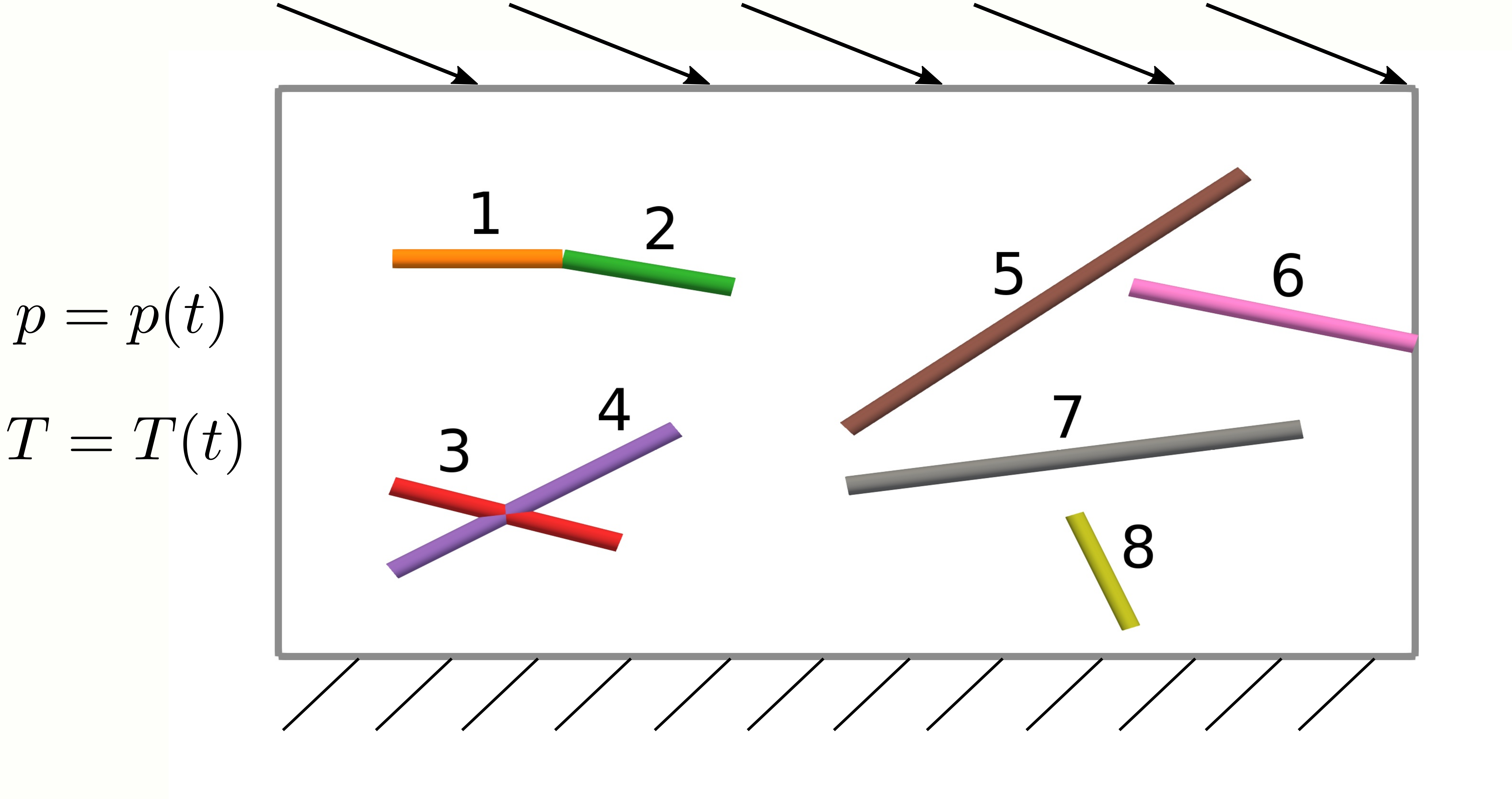
Figure 4: Fracture geometry and the boundary conditions driving the dynamics for examples 1 and 2. The colour scheme for the fractures is used throughout Sections 4.1 and 4.2. The domain is fixed at the bottom and displaced at the top, while temporally varying pressure and temperature values $p_{\partial\Omega}$ and $T_{\partial\Omega}$ are prescribed at the left boundary.

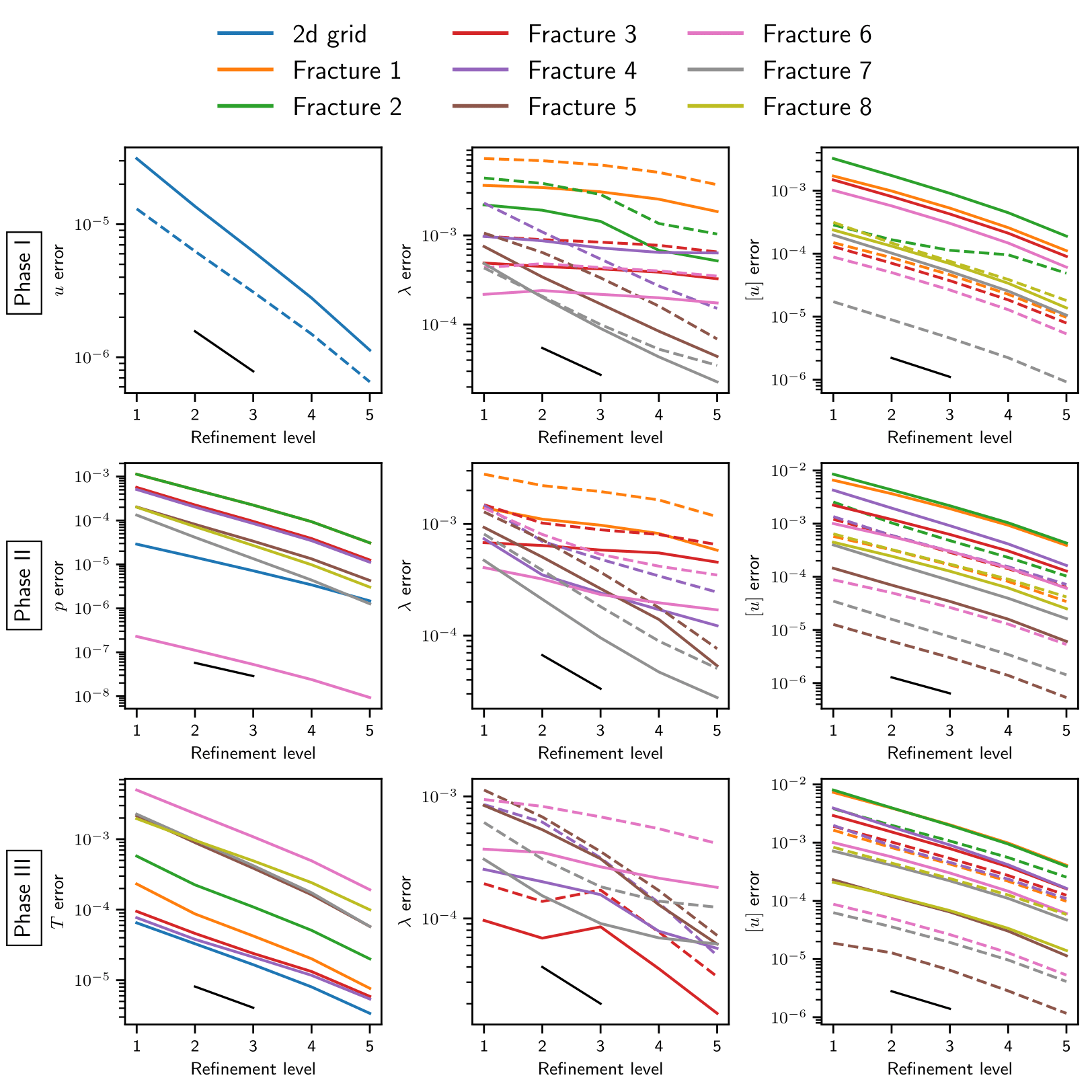
Figure 5: Example 1: Errors relative to reference grid solution for solutions on five coarser grids at the end of the three phases, shown top to bottom. The three columns correspond to the variable of the main driving force, contact traction and displacement jumps. Solid and dashed lines correspond to $x$ and $y$ component in the matrix and tangential and normal component in the fractures. The black lines indicate first order.

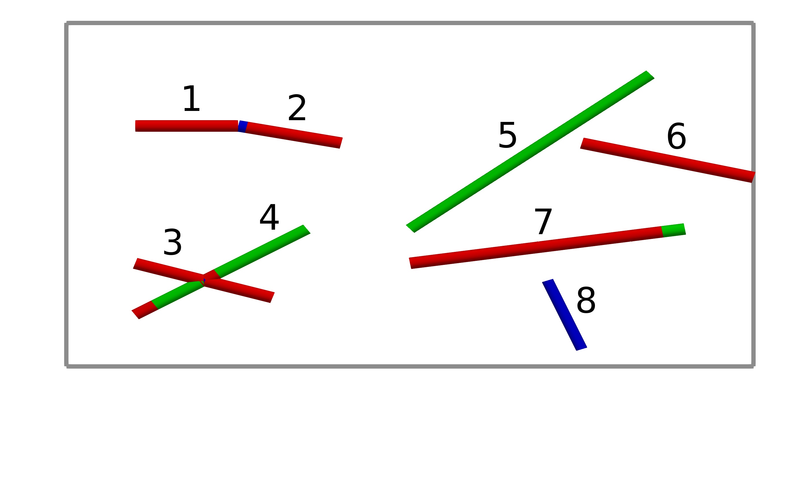
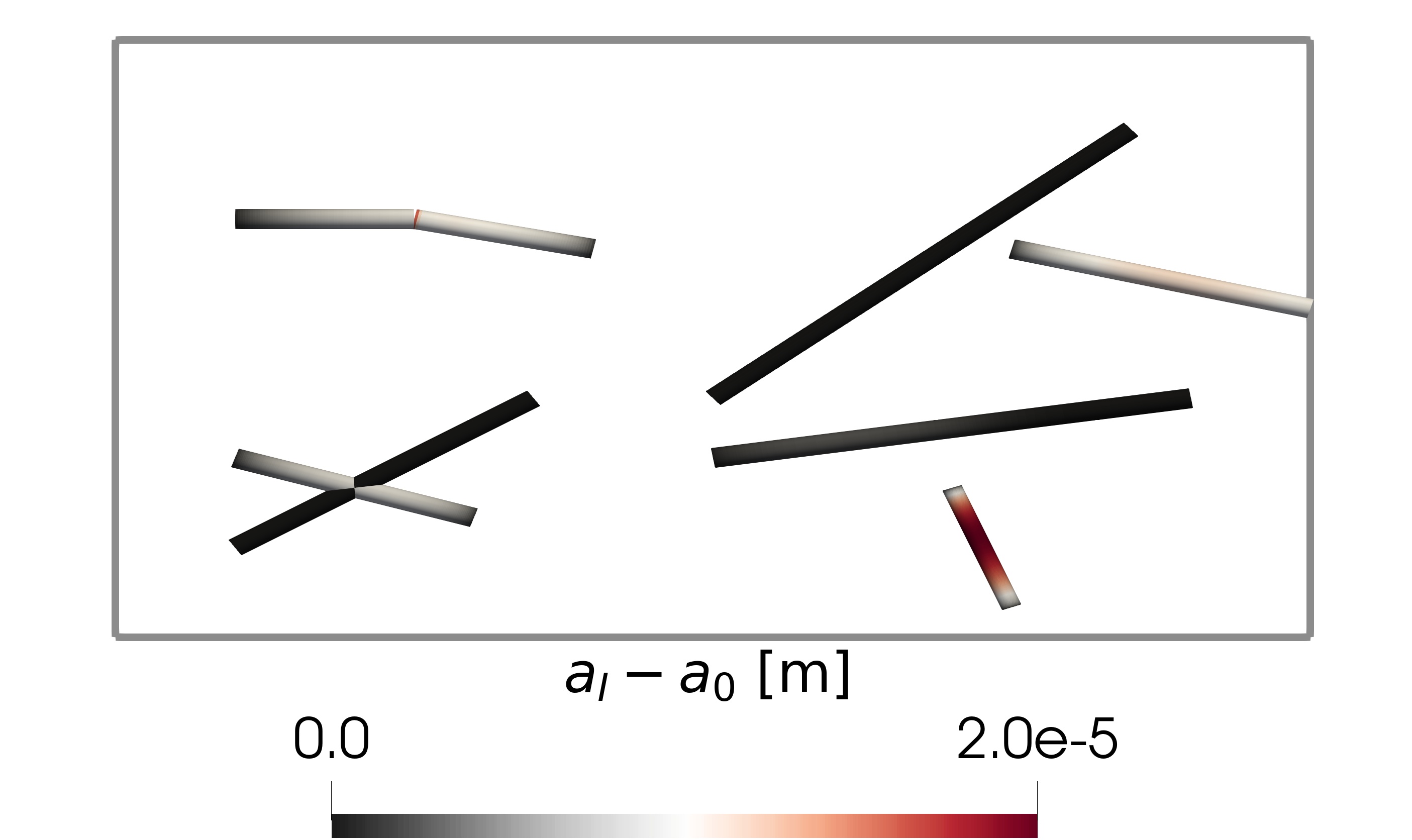
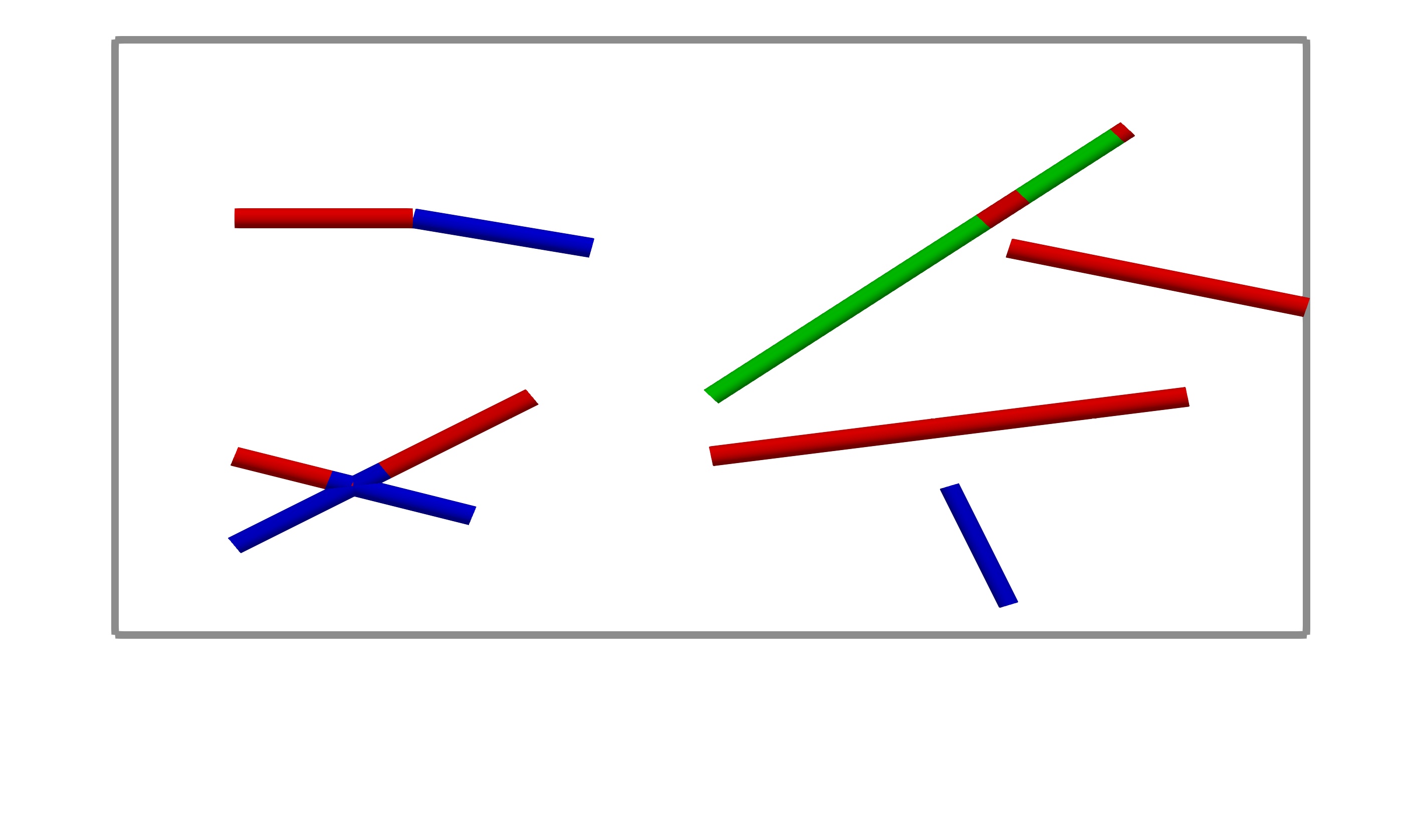
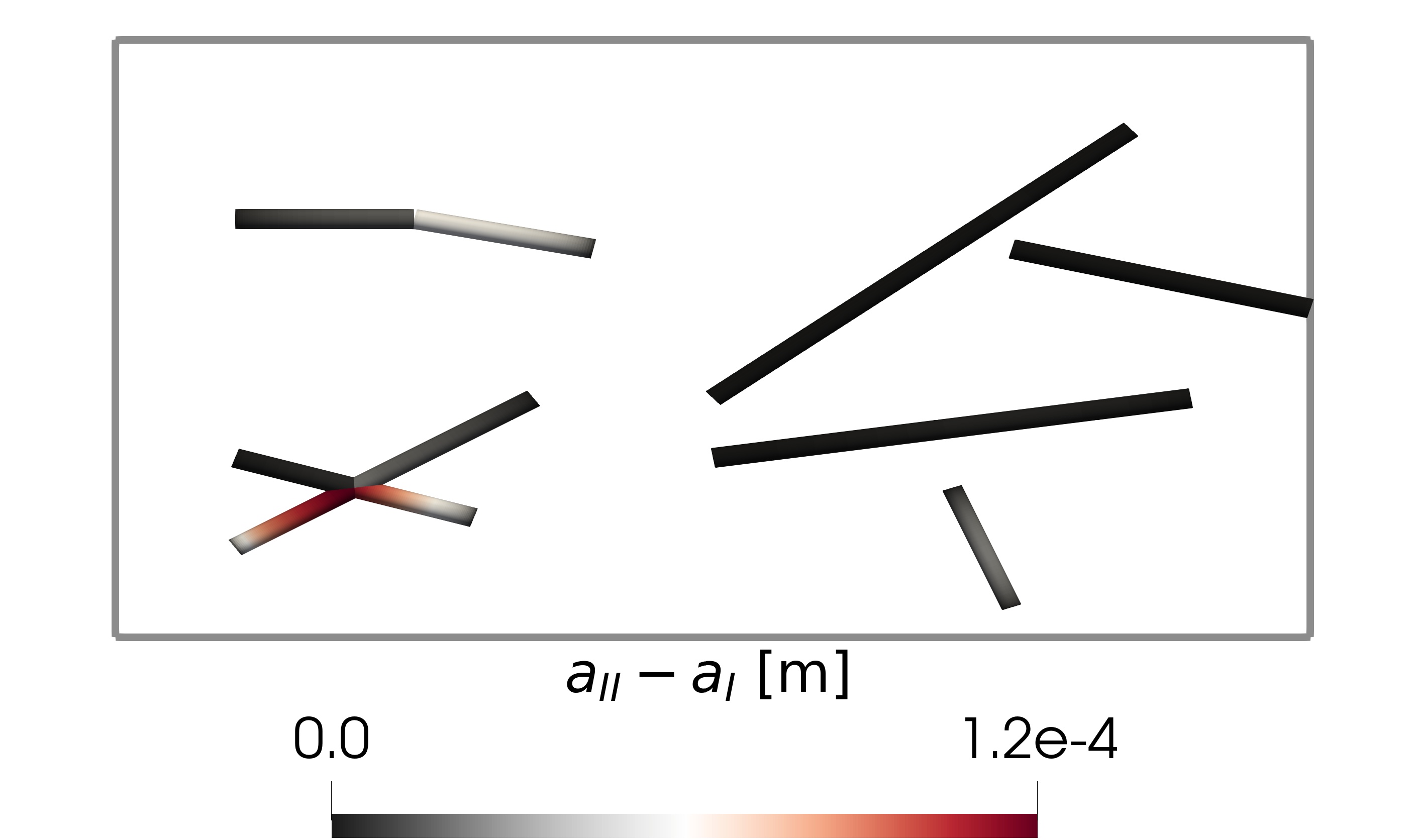
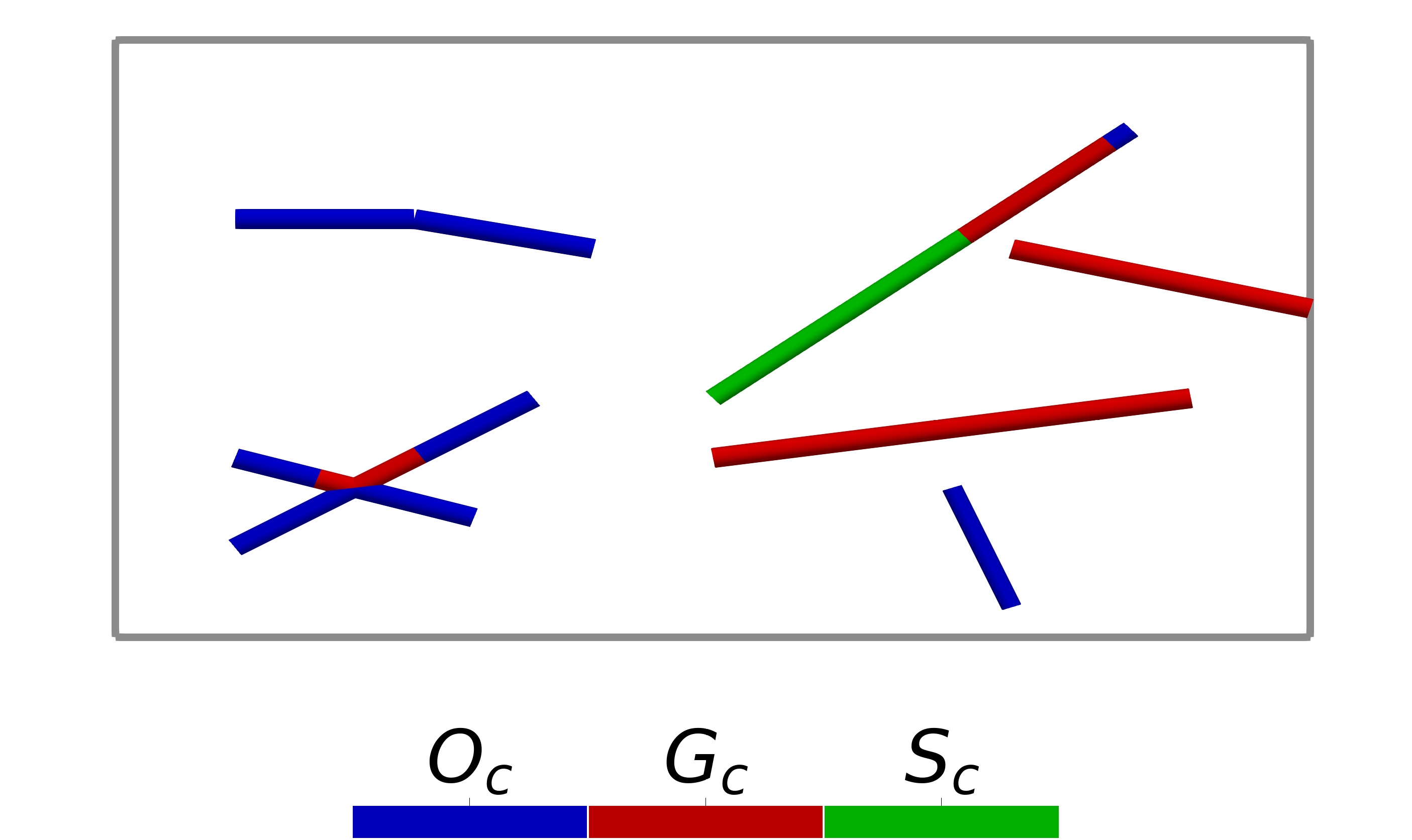
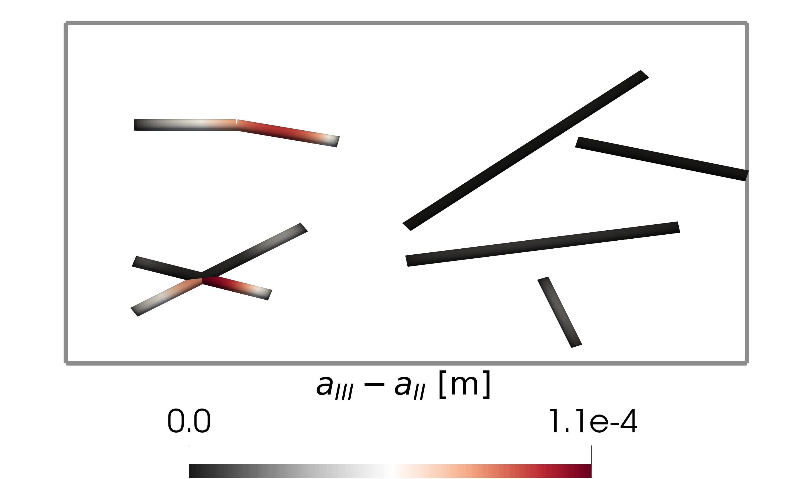
Figure 6: Example 1: Left: Fracture states according to cumulative displacement jumps at the end of phases I through III shown top to bottom. Right: Aperture increments throughout each of the three phases I through III shown top to bottom.

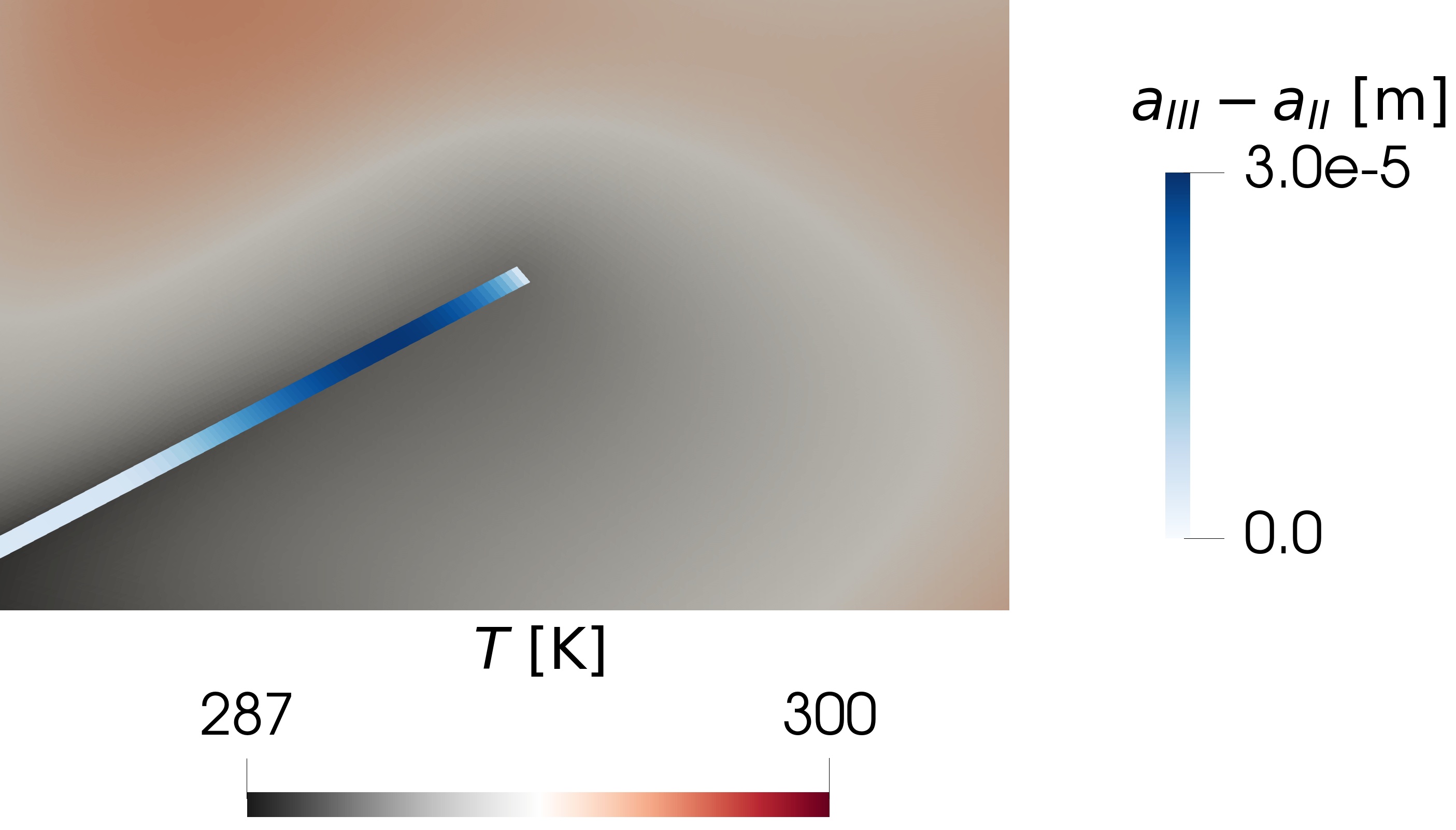
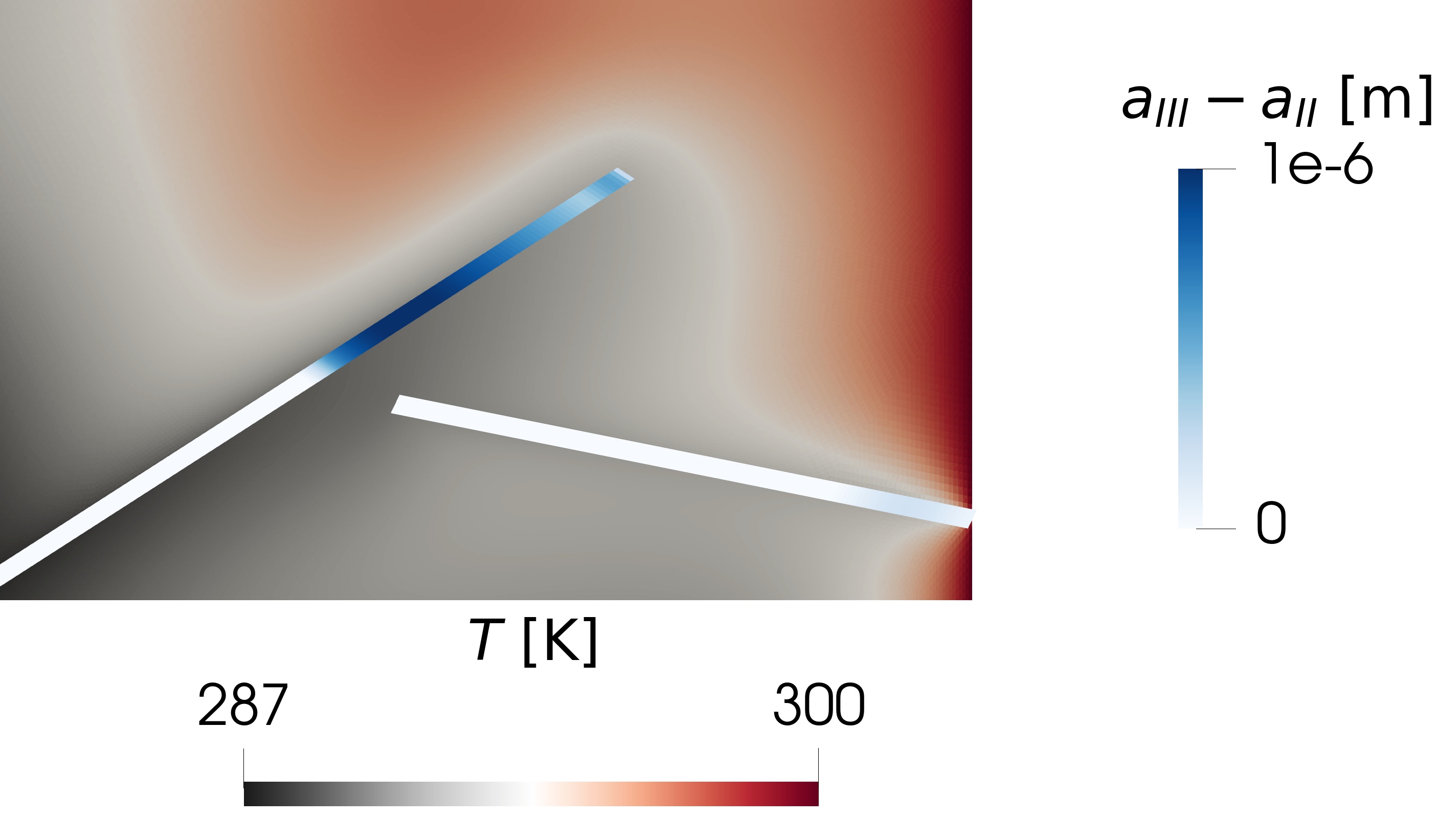
Figure 7: Example 1: Matrix temperature with superimposed fracture aperture increment in the region surrounding fracture 4 (left) and fractures 5 and 6 (right). The temperature solutions are $8\text{/}3\text{\,}\mathrm{h}$ and $22\text{/}3\text{\,}\mathrm{h}$ into phase III, at which point the cold temperature front has not yet moved past the respective regions. The subscripts on $a$ indicate the value at the end of the corresponding phase, i.e. the values are the increments throughout phase III.

Figure 5 shows convergence results for the end of the three phases. For each phase, we plot the errors for three primary variables on individual subdomains for the different refinement levels. The variables are displacement jumps, contact tractions and the variable related to the main driving force of the phase. The error is computed by projecting the cell-centre value of the coarse grids onto the reference grid and then computing the $L^{2}$ norm of the difference between coarse and fine solution. Errors are normalised by the number of reference cells in the subdomain multiplied by a weight $k$ representing the magnitude of the global range of the variable in question. The weights are obtained from the boundary conditions and are $k_{\bm{u}}=||($5\text{\times}{10}^{-4}$,$-2\text{\times}{10}^{-4}$)||$ $\mathrm{m}$, $k_{p}=$ $4\text{\times}{10}^{7}\text{\,}\mathrm{Pa}$, $k_{T}=$$15\text{\,}\mathrm{K}$ and $k_{\bm{\lambda}}=\text{E}k_{\bm{u}}$ with E denoting Young’s modulus.

In general, the expected first order convergence is observed. The exception is traction on some of the fractures (1, 2, 3 and 6). These local errors may be attributed to the geometrical challenges posed by those fractures: Fractures 1 and 2 meet in a kink, which seems to lead to relatively large errors compared to the remaining fractures as discussed by Berge et al. [34]. Fracture 3 intersects fracture 4, while the error on fracture 6 is concentrated around the leftmost tip, which is close to the neighbouring fracture 5. However, the traction solutions converge for all fractures without small transition regions and the challenging geometrical features have no discernible effect on the convergence in the other primary variables. Therefore, taken together, the presented results serve as a verification of the model.

Figure 6 shows the fracture deformation for each of the three phases, and thus demonstrates the effect of each of the three driving forces. The richness in physical processes and the complexity of coupling in the fractured THM problem is well illustrated by a phenomenon observed towards the end of phase III around fractures 5 and 6 (see Fig. 7). The role of fractures as preferential flow pathways leads to high flow rates and cooling in the region where fluid leaves fracture 5, both at the tip closest to the right boundary and in the area closest to fracture 6. This, in turn, leads to local contraction of the matrix and fracture dilation — in this particular case both through shear displacement and normal opening as seen from the final deformation state (bottom left in Fig. 6). The dilation further increasing the fracture conductivity can be expected to enhance the effect, which is also observed at the tip of fracture 4 somewhat earlier in the simulation. This phenomenon of enhanced cooling-induced aperture increase in regions where the fluid enters or leaves a fracture can be expected to be of a general character.

$K_{s}$	Solid bulk modulus	$2.2\text{\times}{10}^{10}\text{\,}\mathrm{Pa}$
$K_{f}$	Fluid bulk modulus	$2.5\text{\times}{10}^{9}\text{\,}{\mathrm{Pa}}^{-1}$
$\mu$	Shear modulus	$1.7\text{\times}{10}^{10}\text{\,}\mathrm{Pa}$
$\eta$	Viscosity	$1.0\text{\times}{10}^{-3}\text{\,}\mathrm{Pa}\text{\,}\mathrm{s}$
$\mathcal{K}$	Permeability	$1.0\text{\times}{10}^{-15}\text{\,}{\mathrm{m}}^{2}$
$\alpha$	Biot coefficient	$0.8$
$F$	Friction coefficient	$0.5$
$\beta_{s}$	Solid thermal expansion	$8.0\text{\times}{10}^{-6}\text{\,}{\mathrm{K}}^{-1}$
$\beta_{f}$	Fluid thermal expansion	$4.0\text{\times}{10}^{-4}\text{\,}{\mathrm{K}}^{-1}$
$\kappa_{s}$	Solid thermal conductivity	$3.0\text{\,}\mathrm{W}\text{\,}{\mathrm{m}}^{-1}\text{\,}{\mathrm{K}}^{-1}$
$\kappa_{f}$	Fluid thermal conductivity	$0.6\text{\,}\mathrm{W}\text{\,}{\mathrm{m}}^{-1}\text{\,}{\mathrm{K}}^{-1}$
$c_{s}$	Solid specific heat capacity	$790\text{\,}\mathrm{J}\text{\,}{\mathrm{K}}^{-1}$
$c_{f}$	Fluid specific heat capacity	$4.2\text{\times}{10}^{3}\text{\,}\mathrm{J}\text{\,}{\mathrm{K}}^{-1}$
$\phi$	Porosity	$1.0\text{\times}{10}^{-2}$
$\rho_{s}$	Solid density	$2.7\text{\times}{10}^{3}\text{\,}\mathrm{kg}\text{\,}{\mathrm{m}}^{-1}$
$\rho_{f,0}$	Reference fluid density	$1.0\text{\times}{10}^{3}\text{\,}\mathrm{kg}\text{\,}{\mathrm{m}}^{-1}$

Table 1: Model parameters for the example simulations.

4.2 Example 2 — Fracture dilation models

The second example is a study of different models for fracture dilation based on simulation of the case described in Section 4.1 with two simplified aperture models. In the first simplification, model 0, there is no coupling between shear displacement and dilation, i.e. $g=0$ and $a=a_{0}+[\![\bm{u}]\!]_{n}$. In the second simplified model (1) the aperture is related to the tangential displacement as $a=a_{0}+[\![\bm{u}]\!]_{n}+\tan(\psi)||[\![\bm{u}]\!]_{\tau}||$ while $g$ is kept constant. This represents a naive one-way coupling which accounts for the dilation effect for the apertures and fracture permeability. We emphasise that neglecting the back-coupling to normal displacement – and thus to the matrix momentum balance – makes this model inconsistent. The model of 4.1, where dilation is coupled to the displacement solution through the gap function according to Eq. (32), represents the full two-way dilation coupling and will be referred to as model 2. Thus, model names correspond to the number of directions of couplings accounted for by the models.

A comparison in terms of the final spatial distribution of aperture increase and tangential displacement jump on each of the closed fractures is shown in Fig. 8. As the dilation relations are irrelevant for open fractures, analysis is based on the mostly closed fractures 5 through 7. Fractures 6 and 7 clearly demonstrate how the dilation coupling in model 2 reduces tangential displacement compared to the simplified methods, as the induced normal displacement increases the normal traction on the fractures. Interestingly, the apertures displayed in Fig. 8 show overestimation for the one-way coupling due to the above-mentioned overestimation of the tangential jumps. Model 0 obviously yields no shear dilation. The model 0 aperture increase of fracture 5 is thus related to the fracture being open. Note that part of this region is closed for model 2 (cf. the bottom left illustration of Fig. 6) demonstrating how inconsistency affects the results beyond the prediction of $a$.

The magnitude of the discrepancy must be expected to depend on rock and fault parameters, particularly the dilation angle. The results demonstrate the strong coupling in the problem, and that compromising this coupling in numerical modelling may lead to significant error in the results.

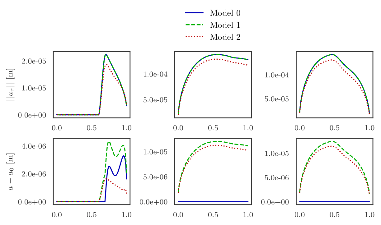
Figure 8: Example 2: Final tangential displacement jumps (top) and apertures (bottom) along the three (partially) closed fractures 5, 6 and 7, corresponding to the three columns left to right. Results are shown for the three different models for the relationship between $a$ and $[\![\bm{u}]\!]$. The cells are sorted from lowest to highest $x$ coordinate.

4.3 Example 3 — Hydraulic stimulation and long-term cooling of a geothermal reservoir

The third example shows hydraulic stimulation of a geothermal reservoir, followed by an injection and production phase leading to long-term reservoir cooling for the three-dimensional geometry in Fig. 9. The domain is the box $($-750\text{\,}\mathrm{m}$,$750\text{\,}\mathrm{m}$)\times($-750\text{\,}\mathrm{m}$,$750\text{\,}\mathrm{m}$)\times($-1750\text{\,}\mathrm{m}$,$-250\text{\,}\mathrm{m}$)$ and contains three fractures, two of which intersect along a line, and two wells. The initial values are $p=p_{H}=\rho_{f,0}Gz$ $\mathrm{Pa}$, $T=T_{0}=$350\text{\,}\mathrm{K}$$ and $a_{0}=$2\text{\times}{10}^{-3}\text{\,}\mathrm{m}$$, with the positive direction of the $z$ axis pointing upwards and $G=$9.81\text{\,}\mathrm{m}\text{\,}{\mathrm{s}}^{-2}$$ denoting the gravitational acceleration. After letting the system reach equilibrium under the mechanical boundary conditions representing an anisotropic background stress in phase I, we simulate a pressure stimulation phase (II) and a production and long-term cooling phase (III). In the 10 hour stimulation phase, the flow rates of the injection and production wells are $75$ and $0\text{\,}\mathrm{L}\text{\,}{\mathrm{s}}^{-1}$, respectively. During the 15 year production phase, both rates are $20\text{\,}\mathrm{L}\text{\,}{\mathrm{s}}^{-1}$. The injection temperature is $70\text{\,}\mathrm{K}$ below the reservoir temperature. The wells are incorporated as source terms in the fracture cells intersected by the well paths, with upwind discretisation for the energy equation in the production cell. Hydrostatic Dirichlet boundary conditions $p=p_{H}$ apply for the pressure. An anisotropic compressive background stress is imposed with the following non-zero stress tensor values

$$\begin{aligned} \sigma_{xx}=\frac{3}{4}\rho_{s}Gz\qquad\sigma_{yy}=\frac{3}{2}\rho_{s}Gz\qquad\sigma_{zz}=\rho_{s}Gz.\end{aligned}$$ (47)

While the remaining parameters listed in the Table 1 are plausible for geothermal reservoirs, they do not correspond to a specific site. The number of Newton iterations required for convergence is below ten for all time steps.

The results are summarised through the temporal evolution of the norm of the displacement jumps on the three fractures shown in Fig. 9. Significant stimulation effects appear in both phase II and phase III, with the magnitude of the jumps somewhat larger during the cooling; dynamics initiate latest on the injection fracture due to its orientation relative to the background stress.

Figure 10 shows spatial plots of pressure, temperature, aperture, displacement jumps and deformation state. The plots demonstrate the model’s cell-wise spatial resolution of the dynamics both in fractures and matrix. For all three phases, displacement jumps are oriented in agreement with the background stress field and are very closely aligned. The only cells in $\mathcal{O}$ are around the intersection in phase III. For the remaining cells, the (relatively small) normal components of the orientation arrows are due solely to shear dilation.

During phase II, aperture increments are most pronounced on fracture 2, which has no wells. However, its intersection with fracture 1 where injection occurs leads to a significant pressure increase. Despite negligible pressure perturbation in fracture 3, some slip is observed due to stress redistribution following the deformation of fracture 2. The location of the slip in fracture 3, away from the stress shadow of fracture 2, highlights the complex mechanical interplay between fractures in a network.

During phase III, some displacement jumps are induced in fracture 1 close to the intersection, whereas there is significant aperture increase throughout fracture 2 as a result of cooling of the surrounding rock. Along fracture 3, the deforming region is different from the previous phase, with displacement occurring in the region closest to fracture 2, where the surrounding matrix has been cooled the most. This conforms with the observations in Section 4.1 of aperture increases in regions of fluid entry or departure from the fractures.

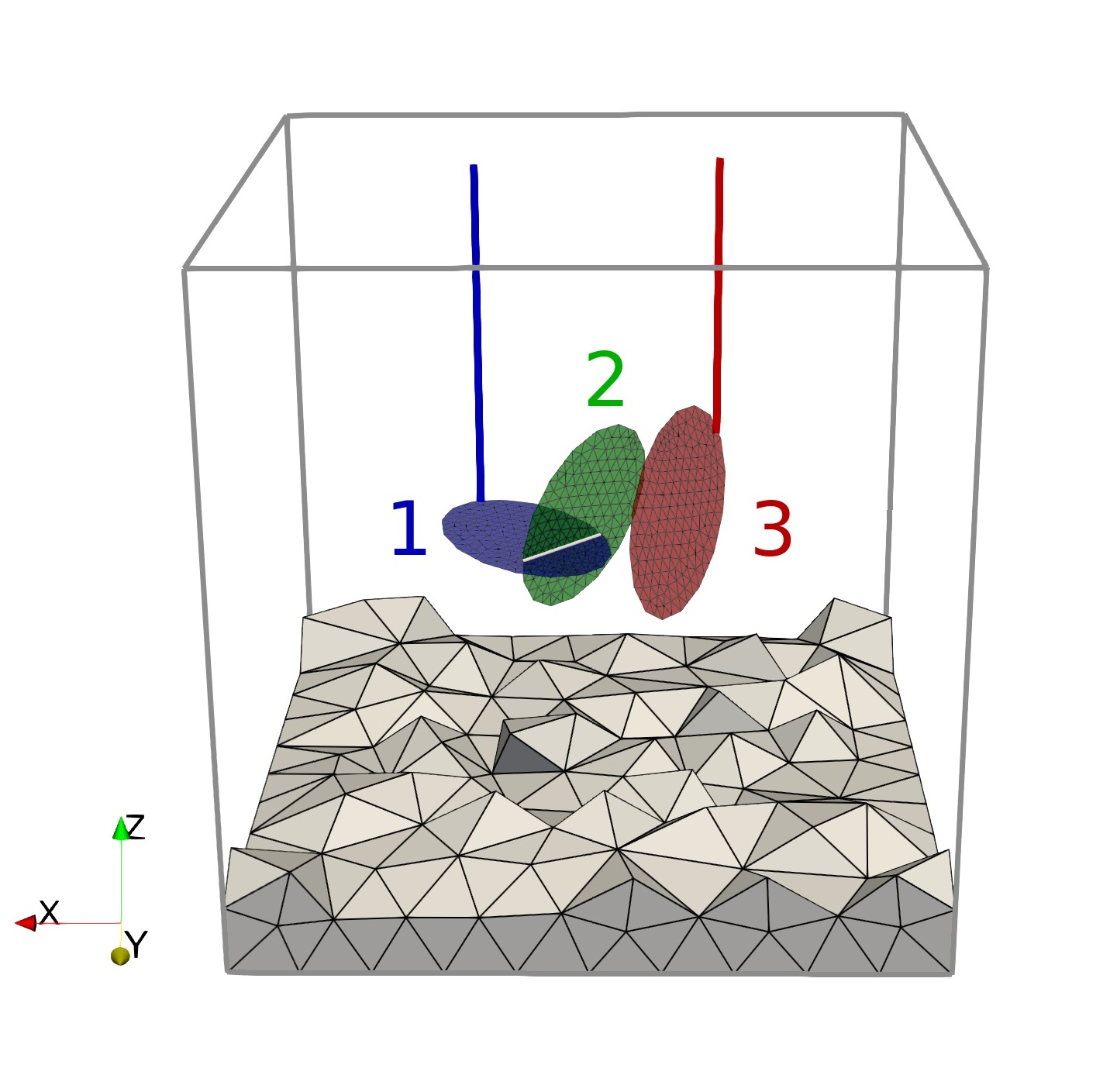
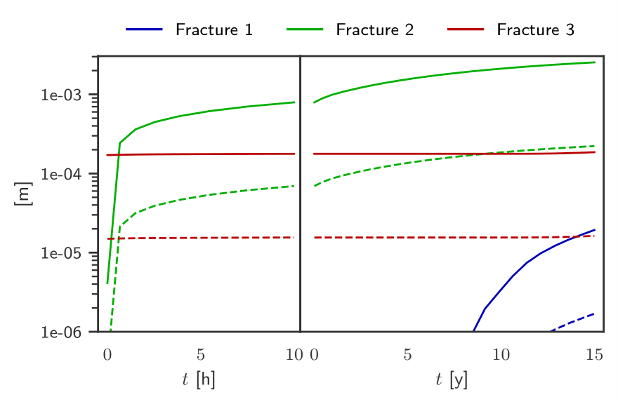
Figure 9: Example 3: Left: Fracture network geometry and well paths. The grey lines indicate the domain boundary and the white line is the 1d fracture intersection, while the injection and production wells are indicated by blue and red lines, respectively. Also shown are the 2d grid cells and some coarse 3d grid cells close to the boundary, indicating grid refinement in the region of interest. Right: $L^{2}$ norm of tangential (solid lines) and normal (dashed lines) displacement jumps on each fracture during phases II and III. The values are normalised by the number of fracture cells. The black dashed line shows the number of Newton iterations needed for convergence.

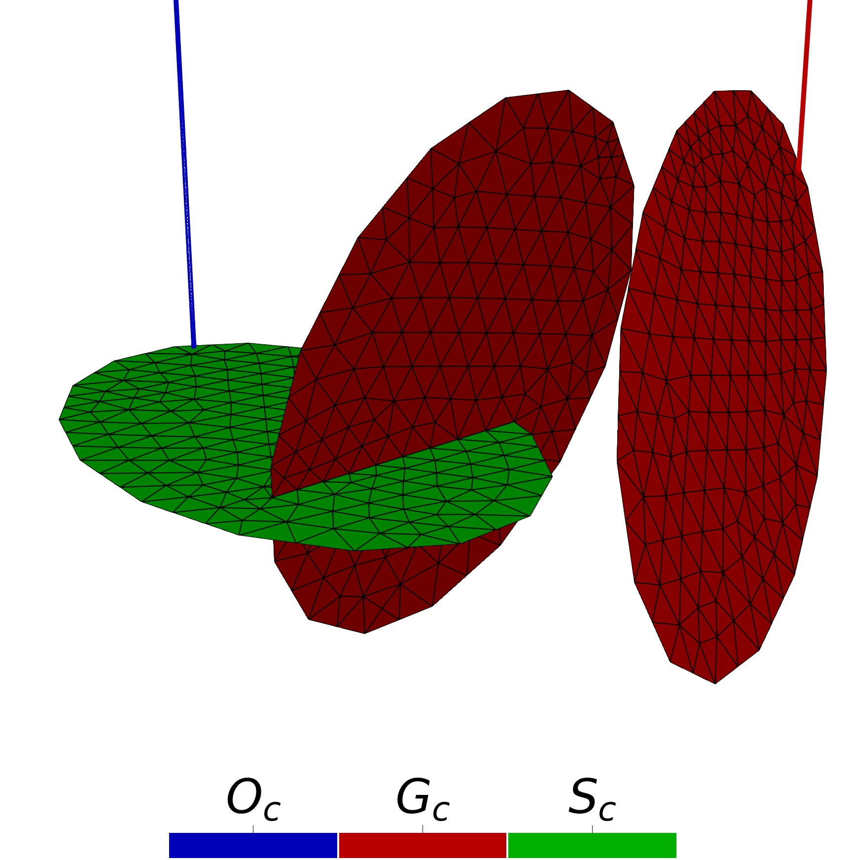
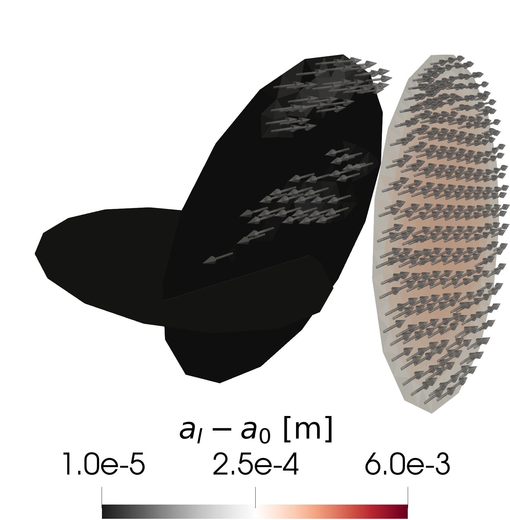
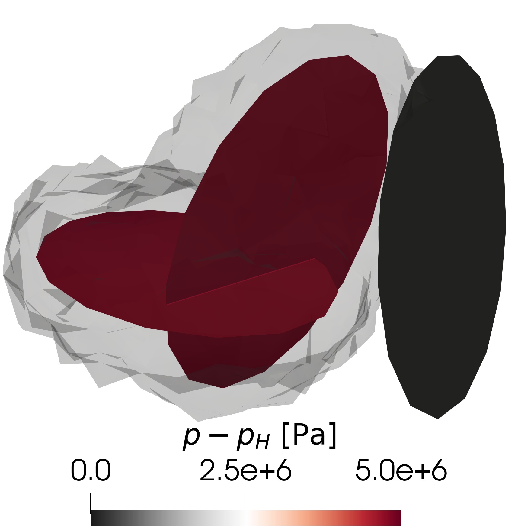
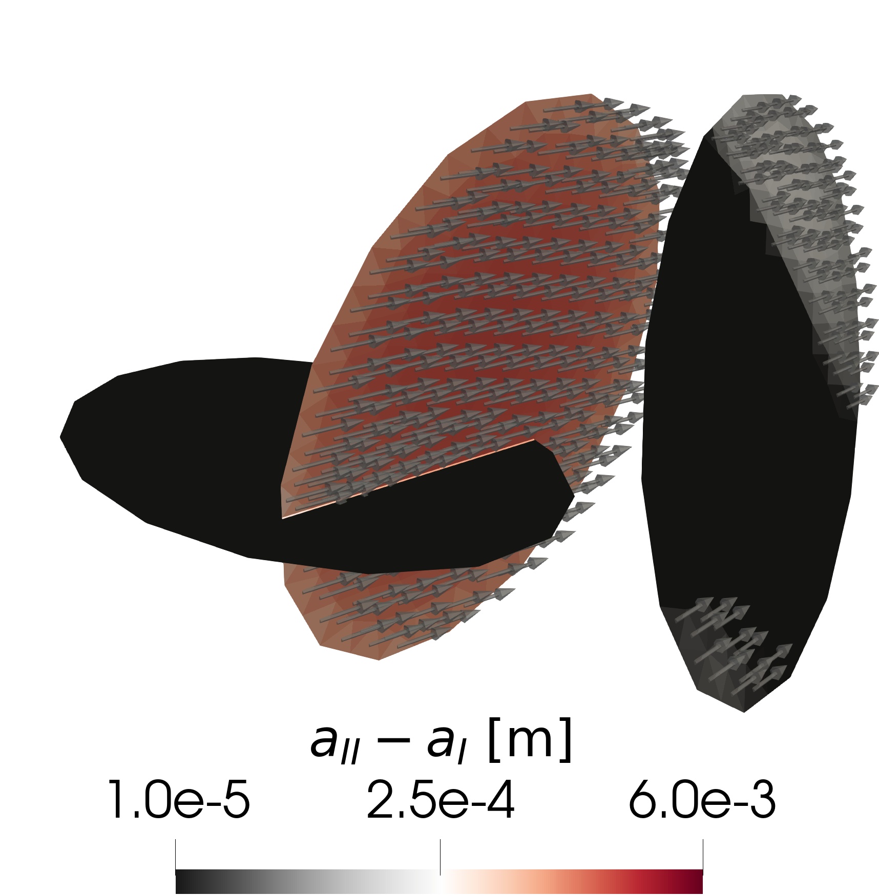
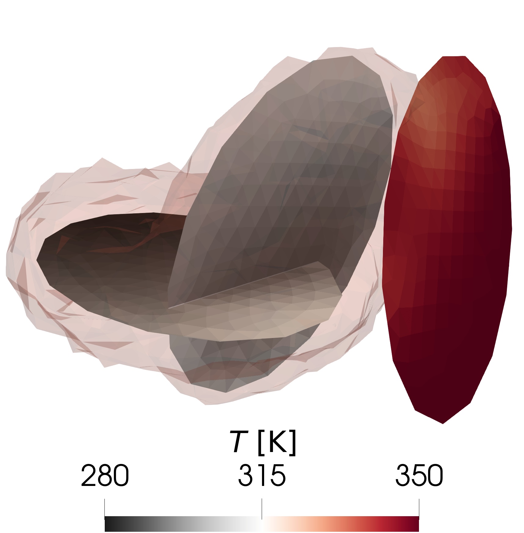
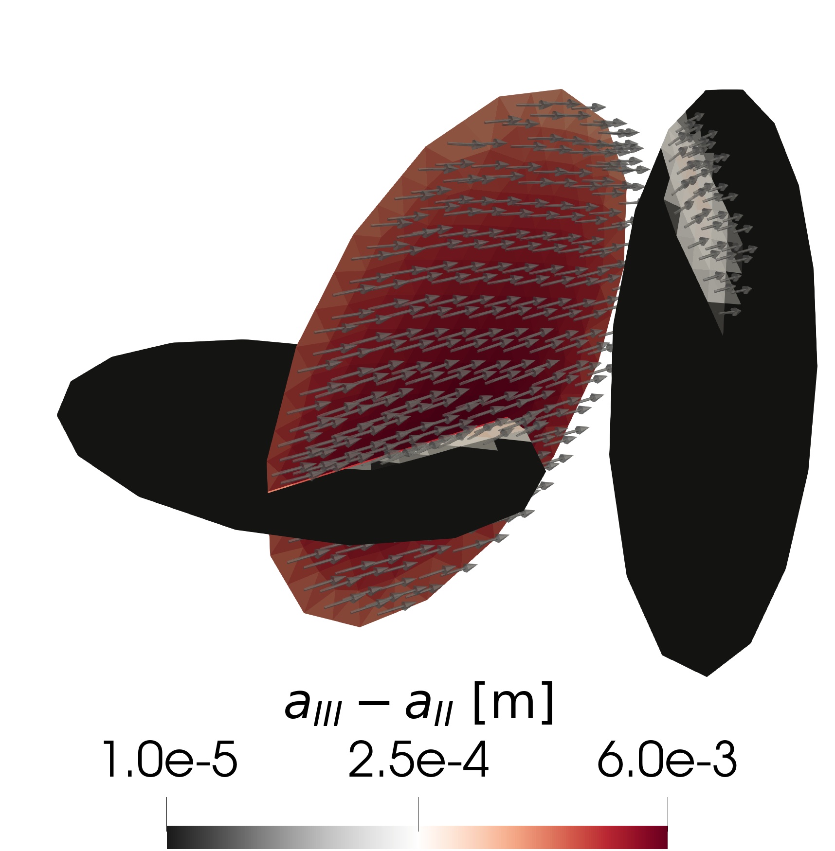
Figure 10: Example 3: Left: Deformation state according to the cumulative displacement jumps at the end of phase I (top). Perturbation from hydrostatic pressure at the end of phase II for the fractures and matrix cells satisfying $p-p_{H}>$5\text{\times}{10}^{5}\text{\,}\mathrm{Pa}$$ (centre). Final fracture temperature and matrix cells satisfying $T-T_{0}<$-15\text{\,}\mathrm{K}$$ (bottom). Right: Aperture increments and displacement jump direction for each of the three phases top to bottom. The arrows show how the side of the fracture which is in view is displaced relative to the side not in view. Note that the logarithmic scale for the aperture increments is truncated at $1\text{\times}{10}^{-5}\text{\,}\mathrm{m}$ for visualisation purposes.

5 Conclusion

A model for fully coupled thermo-hydro-mechanical processes in porous media with deforming fractures is presented. Using the discrete–fracture–matrix approach, the matrix, the fractures and the fracture intersections are represented by subdomains of different dimensions connected by interfaces in a mixed-dimensional model. Balance equations for energy and mass in all subdomains are coupled by fluxes on the interfaces, while the momentum balance in the matrix and traction balance and non-penetration for the fracture surfaces are coupled through interface displacements. These governing equations are supplemented with constitutive laws, including a Coulomb type friction law and a linear shear dilation relation for the fractures. For the latter, a novel model consistently coupling slip and shear dilation of the fractures with the stress response of the matrix is presented. The resulting set of model equations is discretised using cell-centred multi-point finite volume schemes and a semismooth Newton method for fracture deformation and solved fully coupled.

The model and its implementation are verified through a convergence study displaying first-order convergence for all primary variables and subdomains, except for the expected local reduction of convergence in the transition between contact regimes. An exploration of three different shear-dilation models reveals significant discrepancies, demonstrating the importance of accurate and consistent modelling of the underlying physical mechanisms and their couplings.

Investigations of 2d and 3d examples identify a mechanism by which cooling-induced shear dilation preferentially occurs in regions where fluid leaves or enters a fracture. The investigations also show the complexity of the process–structure interactions which may arise: in particular, how fracture deformation and resulting fracture dilation is induced by both mechanical, hydraulic and thermal driving forces. This confirms the need for models which explicitly incorporate all relevant processes and structural features as well as the resulting process–structure interactions. Furthermore, it demonstrates the proposed model’s prowess in capturing such highly complex interactions and identifying their governing mechanisms. Extensions such as chemical processes and more advanced friction models and dilation relations could readily be accommodated in the applied mixed-dimensional framework.

6 Acknowledgements

The authors thank two anonymous reviewers for comments and suggestions which contributed to improving the paper.

Funding: This work was supported by the Research Council of Norway and Equinor ASA through grant number 267908. I. Stefansson and I. Berre also acknowledge funding from the VISTA programme, The Norwegian Academy of Science and Letters.

References

- Pine and Batchelor [1984] R. Pine, A. Batchelor, Downward migration of shearing in jointed rock during hydraulic injections, in: International Journal of Rock Mechanics and Mining Sciences & Geomechanics Abstracts, volume 21, Elsevier, 1984, pp. 249–263.
- Rutqvist and Stephansson [2003] J. Rutqvist, O. Stephansson, The role of hydromechanical coupling in fractured rock engineering, Hydrogeology Journal 11 (2003) 7–40.
- Evans et al. [2005] K. Evans, H. Moriya, H. Niitsuma, R. Jones, W. Phillips, A. Genter, J. Sausse, R. Jung, R. Baria, Microseismicity and permeability enhancement of hydrogeologic structures during massive fluid injections into granite at 3 km depth at the Soultz HDR site, Geophysical Journal International 160 (2005) 388–412.
- Keranen et al. [2014] K. M. Keranen, M. Weingarten, G. A. Abers, B. A. Bekins, S. Ge, Sharp increase in central Oklahoma seismicity since 2008 induced by massive wastewater injection, Science 345 (2014) 448–451.
- De Waal et al. [2015] J. De Waal, A. Muntendam-Bos, J. Roest, Production induced subsidence and seismicity in the Groningen gas field - can it be managed?, Proceedings of the International Association of Hydrological Sciences 372 (2015) 129.
- Improta et al. [2015] L. Improta, L. Valoroso, D. Piccinini, C. Chiarabba, A detailed analysis of wastewater-induced seismicity in the Val d’Agri oil field (Italy), Geophysical Research Letters 42 (2015) 2682–2690.
- Keranen and Weingarten [2018] K. M. Keranen, M. Weingarten, Induced seismicity, Annual Review of Earth and Planetary Sciences (2018).
- Dorbath et al. [2009] L. Dorbath, N. Cuenot, A. Genter, M. Frogneux, Seismic response of the fractured and faulted granite of Soultz-sous-Forêts (France) to 5 km deep massive water injections, Geophysical Journal International 177 (2009) 653–675.
- Ellsworth et al. [2019] W. L. Ellsworth, D. Giardini, J. Townend, S. Ge, T. Shimamoto, Triggering of the Pohang, Korea, Earthquake (m w 5.5) by Enhanced Geothermal System Stimulation, Seismological Research Letters 90 (2019) 1844–1858.
- Häring et al. [2008] M. O. Häring, U. Schanz, F. Ladner, B. C. Dyer, Characterisation of the basel 1 enhanced geothermal system, Geothermics 37 (2008) 469–495.
- Karimi-Fard et al. [2003] M. Karimi-Fard, L. J. Durlofsky, K. Aziz, An Efficient Discrete-Fracture Model Applicable for General-Purpose Reservoir Simulators, SPE Journal 9 (2003) 227–236.
- Martin et al. [2005] V. Martin, J. Jaffré, J. E. Roberts, Modeling Fractures and Barriers as Interfaces for Flow in Porous Media, SIAM J. Sci. Comput. 26 (2005) 1667–1691. doi:10.1137/S1064827503429363.
- Reichenberger et al. [2006] V. Reichenberger, H. Jakobs, P. Bastian, R. Helmig, A mixed-dimensional finite volume method for two-phase flow in fractured porous media, Advances in Water Resources 29 (2006) 1020–1036.
- Nordbotten et al. [2019] J. M. Nordbotten, W. M. Boon, A. Fumagalli, E. Keilegavlen, Unified approach to discretization of flow in fractured porous media, Computational Geosciences 23 (2019) 225–237.
- Rutqvist et al. [2008] J. Rutqvist, J. Birkholzer, C.-F. Tsang, Coupled reservoir–geomechanical analysis of the potential for tensile and shear failure associated with CO2 injection in multilayered reservoir–caprock systems, International Journal of Rock Mechanics and Mining Sciences 45 (2008) 132–143.
- Rutqvist et al. [2013] J. Rutqvist, A. P. Rinaldi, F. Cappa, G. J. Moridis, Modeling of fault reactivation and induced seismicity during hydraulic fracturing of shale-gas reservoirs, Journal of Petroleum Science and Engineering 107 (2013) 31–44.
- Wassing et al. [2014] B. Wassing, J. Van Wees, P. Fokker, Coupled continuum modeling of fracture reactivation and induced seismicity during enhanced geothermal operations, Geothermics 52 (2014) 153–164.
- Cappa and Rutqvist [2011] F. Cappa, J. Rutqvist, Modeling of coupled deformation and permeability evolution during fault reactivation induced by deep underground injection of CO2, International Journal of Greenhouse Gas Control 5 (2011) 336–346.
- Ucar et al. [2018] E. Ucar, I. Berre, E. Keilegavlen, Three-dimensional numerical modeling of shear stimulation of fractured reservoirs, Journal of Geophysical Research: Solid Earth 123 (2018) 3891–3908.
- Ferronato et al. [2008] M. Ferronato, G. Gambolati, C. Janna, P. Teatini, Numerical modelling of regional faults in land subsidence prediction above gas/oil reservoirs, International journal for numerical and analytical methods in geomechanics 32 (2008) 633–657.
- Gallyamov et al. [2018] E. Gallyamov, T. Garipov, D. Voskov, P. Van den Hoek, Discrete fracture model for simulating waterflooding processes under fracturing conditions, International Journal for Numerical and Analytical Methods in Geomechanics 42 (2018) 1445–1470.
- Shapiro and Andersson [1985] A. M. Shapiro, J. Andersson, Simulation of steady-state flow in three-dimensional fracture networks using the boundary-element method, Advances in Water Resources 8 (1985) 106–110.
- Long et al. [1985] J. C. Long, P. Gilmour, P. A. Witherspoon, A model for steady fluid flow in random three-dimensional networks of disc-shaped fractures, Water Resources Research 21 (1985) 1105–1115.
- Willis-Richards et al. [1996] J. Willis-Richards, K. Watanabe, H. Takahashi, Progress toward a stochastic rock mechanics model of engineered geothermal systems, Journal of Geophysical Research: Solid Earth 101 (1996) 17481–17496.
- Rahman et al. [2002] M. K. Rahman, M. M. Hossain, S. S. Rahman, A shear-dilation-based model for evaluation of hydraulically stimulated naturally fractured reservoirs, International Journal for Numerical and Analytical Methods in Geomechanics 26 (2002) 469–497. doi:10.1002/nag.208.
- Kohl and Mégel [2007] T. Kohl, T. Mégel, Predictive modeling of reservoir response to hydraulic stimulations at the European EGS site Soultz-sous-Forêts, International Journal of Rock Mechanics and Mining Sciences 44 (2007) 1118–1131.
- Bruel [2007] D. Bruel, Using the migration of the induced seismicity as a constraint for fractured hot dry rock reservoir modelling, International Journal of Rock Mechanics and Mining Sciences 44 (2007) 1106–1117.
- Baisch et al. [2010] S. Baisch, R. Vörös, E. Rothert, H. Stang, R. Jung, R. Schellschmidt, A numerical model for fluid injection induced seismicity at Soultz-sous-Forêts, International Journal of Rock Mechanics and Mining Sciences 47 (2010) 405–413.
- McClure and Horne [2011] M. W. McClure, R. N. Horne, Investigation of injection-induced seismicity using a coupled fluid flow and rate/state friction model, Geophysics 76 (2011) WC181–WC198.
- Norbeck et al. [2016] J. H. Norbeck, M. W. McClure, J. W. Lo, R. N. Horne, An embedded fracture modeling framework for simulation of hydraulic fracturing and shear stimulation, Computational Geosciences 20 (2016) 1–18.
- Ciardo and Lecampion [2019] F. Ciardo, B. Lecampion, Effect of dilatancy on the transition from aseismic to seismic slip due to fluid injection in a fault, Journal of Geophysical Research: Solid Earth 124 (2019) 3724–3743.
- McClure [2015] M. W. McClure, Generation of large postinjection-induced seismic events by backflow from dead-end faults and fractures, Geophysical Research Letters 42 (2015) 6647–6654.
- Franceschini et al. [2020] A. Franceschini, N. Castelletto, J. A. White, H. A. Tchelepi, Algebraically stabilized lagrange multiplier method for frictional contact mechanics with hydraulically active fractures, Computer Methods in Applied Mechanics and Engineering 368 (2020) 113161. doi:10.1016/j.cma.2020.113161.
- Berge et al. [2020] R. L. Berge, I. Berre, E. Keilegavlen, J. M. Nordbotten, B. Wohlmuth, Finite volume discretization for poroelastic media with fractures modeled by contact mechanics, International Journal for Numerical Methods in Engineering 121 (2020) 644–663. doi:10.1002/nme.6238.
- Jha and Juanes [2014] B. Jha, R. Juanes, Coupled multiphase flow and poromechanics: A computational model of pore pressure effects on fault slip and earthquake triggering, Water Resources Research 50 (2014) 3776–3808.
- Garipov et al. [2016] T. Garipov, M. Karimi-Fard, H. Tchelepi, Discrete fracture model for coupled flow and geomechanics, Computational Geosciences 20 (2016) 149–160.
- Settgast et al. [2017] R. R. Settgast, P. Fu, S. D. Walsh, J. A. White, C. Annavarapu, F. J. Ryerson, A fully coupled method for massively parallel simulation of hydraulically driven fractures in 3-dimensions, International Journal for Numerical and Analytical Methods in Geomechanics 41 (2017) 627–653. doi:10.1002/nag.2557.
- Ucar et al. [2017] E. Ucar, I. Berre, E. Keilegavlen, Postinjection normal closure of fractures as a mechanism for induced seismicity, Geophysical Research Letters 44 (2017) 9598–9606.
- Wriggers and Zavarise [2004] P. Wriggers, G. Zavarise, Computational contact mechanics, Encyclopedia of computational mechanics (2004).
- Ghassemi and Zhou [2011] A. Ghassemi, X. Zhou, A three-dimensional thermo-poroelastic model for fracture response to injection/extraction in enhanced geothermal systems, Geothermics 40 (2011) 39–49.
- Pandey et al. [2017] S. Pandey, A. Chaudhuri, S. Kelkar, A coupled thermo-hydro-mechanical modeling of fracture aperture alteration and reservoir deformation during heat extraction from a geothermal reservoir, Geothermics 65 (2017) 17–31.
- Salimzadeh et al. [2018] S. Salimzadeh, A. Paluszny, H. M. Nick, R. W. Zimmerman, A three-dimensional coupled thermo-hydro-mechanical model for deformable fractured geothermal systems, Geothermics 71 (2018) 212 – 224. doi:10.1016/j.geothermics.2017.09.012.
- Garipov and Hui [2019] T. Garipov, M. Hui, Discrete fracture modeling approach for simulating coupled thermo-hydro-mechanical effects in fractured reservoirs, International Journal of Rock Mechanics and Mining Sciences 122 (2019) 104075. doi:10.1016/j.ijrmms.2019.104075.
- Keilegavlen et al. [2020] E. Keilegavlen, R. Berge, A. Fumagalli, M. Starnoni, I. Stefansson, J. Varela, I. Berre, Porepy: An open-source software for simulation of multiphysics processes in fractured porous media, Computational Geosciences (2020).
- McTigue [1986] D. McTigue, Thermoelastic response of fluid-saturated porous rock, Journal of Geophysical Research: Solid Earth 91 (1986) 9533–9542.
- Coussy [2004] O. Coussy, Poromechanics, Wiley, 2004.
- Tong et al. [2010] F. Tong, L. Jing, R. W. Zimmerman, A fully coupled thermo-hydro-mechanical model for simulating multiphase flow, deformation and heat transfer in buffer material and rock masses, International Journal of Rock Mechanics and Mining Sciences 47 (2010) 205–217.
- Cacace and Jacquey [2017] M. Cacace, A. B. Jacquey, Flexible parallel implicit modelling of coupled thermal–hydraulic–mechanical processes in fractured rocks, Solid Earth 8 (2017) 921–941.
- Hossain et al. [2002] M. Hossain, M. Rahman, S. Rahman, et al., A shear dilation stimulation model for production enhancement from naturally fractured reservoirs, SPE Journal 7 (2002) 183–195.
- Zimmerman and Bodvarsson [1996] R. W. Zimmerman, G. S. Bodvarsson, Hydraulic conductivity of rock fractures, Transport in porous media 23 (1996) 1–30.
- Davis [2004] T. A. Davis, Algorithm 832: Umfpack v4.3—an unsymmetric-pattern multifrontal method, ACM Trans. Math. Softw. 30 (2004) 196–199. doi:10.1145/992200.992206.
- Franceschini et al. [2019] A. Franceschini, N. Castelletto, M. Ferronato, Block preconditioning for fault/fracture mechanics saddle-point problems, Computer Methods in Applied Mechanics and Engineering 344 (2019) 376–401.
- Both et al. [2019] J. W. Both, K. Kumar, J. M. Nordbotten, F. A. Radu, The gradient flow structures of thermo-poro-visco-elastic processes in porous media, arXiv preprint arXiv:1907.03134 (2019).
- Geuzaine and Remacle [2009] C. Geuzaine, J.-F. Remacle, Gmsh: A 3-d finite element mesh generator with built-in pre- and post-processing facilities, International Journal for Numerical Methods in Engineering 79 (2009) 1309–1331. doi:10.1002/nme.2579.
- Aavatsmark [2002] I. Aavatsmark, An introduction to multipoint flux approximations for quadrilateral grids, Computational Geosciences 6 (2002) 405–432. doi:10.1023/A:1021291114475.
- Nordbotten [2014] J. M. Nordbotten, Cell-centered finite volume discretizations for deformable porous media, International Journal for Numerical Methods in Engineering 100 (2014) 399–418. doi:10.1002/nme.4734.
- Nordbotten [2016] J. Nordbotten, Stable cell-centered finite volume discretization for biot equations, SIAM Journal on Numerical Analysis 54 (2016) 942–968. doi:10.1137/15M1014280.
- Nordbotten and Keilegavlen [2020] J. Nordbotten, E. Keilegavlen, An introduction to multi-point flux (mpfa) and stress (mpsa) finite volume methods for thermo-poroelasticity, arXiv preprint arXiv:2001.01990 (2020).
- Hüeber et al. [2008] S. Hüeber, G. Stadler, B. I. Wohlmuth, A primal-dual active set algorithm for three-dimensional contact problems with coulomb friction, SIAM Journal on Scientific Computing 30 (2008) 572–596.
- Wohlmuth [2011] B. Wohlmuth, Variationally consistent discretization schemes and numerical algorithms for contact problems, Acta Numerica 20 (2011) 569–734. doi:10.1017/S0962492911000079.
- por [2021] Run scripts for porepy simulations, https://github.com/IvarStefansson/A-fully-coupled-numerical-model-of-thermo-hydro-mechanical-processes-and-fracture-contact-mechanics-, 2021.