Fitting continuum wavefunctions with complex Gaussians: Computation of ionization cross sections

Abstract

We implement a full nonlinear optimization method to fit continuum states with complex Gaussians. The application to a set of regular scattering Coulomb functions allows us to validate the numerical feasibility, to explore the range of convergence of the approach, and to demonstrate the relative superiority of complex over real Gaussian expansions. We then consider the photoionization of atomic hydrogen, and ionization by electron impact in the first Born approximation, for which the closed form cross sections serve as a solid benchmark. Using the proposed complex Gaussian representation of the continuum combined with a real Gaussian expansion for the initial bound state, all necessary matrix elements within a partial wave approach become analytical. The successful numerical comparison illustrates that the proposed all-Gaussian approach works efficiently for ionization processes of one-center targets.

Keywords: Continuum wavefunctions, Real Gaussians, Complex Gaussians, Non-linear optimization, Ionization.  

We propose an all-Gaussian approach for electronic scattering processes with one-center targets. Gaussian functions are used not only to describe the initial bound states, but also to represent the final continuum states involved in processes such as photoionization or electron impact ionization. An efficient nonlinear optimization is performed to fit continuum wavefunctions with complex Gaussian representations and once the fitting is done, all integrals necessary to compute cross-sections become analytical.

1 Introduction

As early as $1950$ Boys ¹ emphasized the importance of Gaussians to simplify the calculation of multicenter integrals arising in the study of polyatomic molecular electronic states. One key property is the notorious Gaussian product theorem. For an overview of the use of Gaussian sets in molecular calculations see, e.g., reference ². The optimal set depends very much on the studied problem, e.g., system energy minimization, calculation of resonance states,…. Usually, to avoid a full nonlinear optimization, one may consider a particular choice of exponents such as even-tempered sets ^{3, 4}, well-tempered sets ⁵, random-tempered sets ⁶ or polynomial expansions ⁷. In the $60$s many studies have been dedicated to the representation of bound states by a real Gaussian combination ^{8, 9, 10, 11, 12, 13}. Despite their too fast decay at large distances, Gaussians manage to rather well reproduce molecular electronic orbitals over the physically relevant radial regions ¹⁴. Another drawback is their mathematical inability to reproduce the correct cusp near the origin, an issue that is generally addressed numerically using a combination of Gaussians with large exponents ⁸.

While Gaussians are pretty good for reproducing low-lying bound states, representing on large radial domains multinode states (highly excited or Rydberg states), or highly oscillating continuum states by nodeless Gaussians is numerically very challenging. In spite of the numerous potential applications (such as photoionization ^{15, 16, 17, 18}, high harmonic generation ^{19, 20, 21}, ionization by particle impact ²²) only few exploratory studies have been made ^{23, 24, 25, 26}. Kaufmann et al ²³ optimized a set of Gaussians to represent continuum functions with a reasonable accuracy up to $0.2~{}a.u.$ by the diagonalization of the attractive Coulomb Hamiltonian represented in a finite set of Gaussian-type functions. Nestmann and Peyerimhoff ²⁴ proposed a least square approach to represent Bessel functions with real Gaussians. Faure et al ²⁵ applied the same approach to fit Bessel and Coulomb functions. However, the fitting error for large energies (typically $\approx 3$ Rydbergs) is visible to the naked eye. Fiori and Miraglia ²⁶ optimized Gaussians to fit distortion functions by first removing the dominant fast oscillatory plane wave from the Coulomb function. An alternative approach to reproduce the oscillating behavior of continuum states is to add to Gaussian sets some supplementary functions, like B-splines ¹⁵.

We believe that expansions in complex Gaussians, that it to say Gaussians with complex exponents, offer an alternative and possibly more suitable way of representing continuum states. Complex Gaussians have already been proven to be successful in resonance stabilization calculations, where they arise from a complex scaling transformation ^{27, 28, 29, 30}. Such functions possess an intrinsically oscillatory behavior that may facilitate the task of representing continuum states over larger radial domains. Previous investigation in this line, include the work of Matsuzaki et al who used complex Slater orbitals ³¹ and complex Gaussians ³² in photoionization calculations. To represent the outgoing Coulomb function with complex Gaussians, they employed Prony’s method used earlier by Huzinaga ⁸. The main drawback of this method is that it cannot cover all the necessary radial ranges because the radial grid must satisfy a specific square root distribution. This is why in ³² a clear difference is visible between the exact continuum function and its complex fitting in the range $0<r<5~{}a.u.$. Matsuzaki et al also optimized complex Gaussian sets to fit complex Slater functions ³³. The first aim of the present study is to explore further the capacity of complex Gaussians sets to represent continuum states by proposing and implementing a full nonlinear optimization method. In order to test its limitations and range of applicability we take, as an illustration, a set of regular radial Coulomb functions with different energies; the same can be done with any one-electron continuum function as, for example, a numerically generated distorted wave. We also highlight situations where real Gaussians become insufficiently accurate, and point out the advantage of using complex Gaussians instead.

The second purpose of this manuscript is to demonstrate the advantage of such Gaussian representation when evaluating, for example, ionization cross sections. The key idea is to propose an all-Gaussian approach which allows one to analytically evaluate all necessary integrals. It is very well known that using Gaussians to represent bound states renders most of the necessary integrals analytical, a feature that is especially important in the molecular multicenter case by applying the Gaussian product theorem. One question naturally arises: is it possible to exploit such analytical advantages also when continuum states are involved? If they are represented by standard real Gaussians, the answer is obviously positive. What about complex Gaussians? Is the Gaussian product theorem still applicable? It can be easily verified that when complex exponents are present, the product of two Gaussians with different centers will lead to a Gaussian centered at some complex position. Clearly the latter has no physical sense, but it is not a mathematical obstacle for performing multicenter integrals as shown by Kuang and Lin ^{34, 35}. While our long-term goal is to deal with molecular systems, as a first step we consider here the one-center, atomic, case to put our all-Gaussian proposal on solid grounds. To this effect we consider some one-electron matrix elements $\braket{\psi_{\mathbf{k_{e}}}^{-}(\mathbf{r})}{\widehat{O}}{\phi_{i}(\mathbf{r})}$ corresponding to a transition from an initial state $\phi_{i}(\mathbf{r})$ to a continuum state $\psi_{\mathbf{k_{e}}}^{-}(\mathbf{r})$ with ejected electron’s momentum $k_{e}$; the bound-continuum transition occurs via an ionization process represented by some operator $\widehat{O}$. To envisage an all-Gaussian integration approach, the main difficulty stands in a numerically robust representation of the continuum wavefunction by a set of Gaussian functions, and this up to a sufficiently large radial distance. We shall show that thereafter all integrations can be performed analytically with either real or complex sets. As indicated above, we consider here the one-center case and take hydrogen as a benchmark since its ionization cross sections are known exactly for the photon impact case and also, within the first Born approximation, for the electron impact case.

In section 2 we present the algorithm that performs the fitting. The numerical method, based on the approach of Nestmann and Peyerimhoff ²⁴, has been improved here on several aspects, by using a better optimization method and extending it to deal with complex Gaussians. We compare different fitting options with real or complex Gaussians and we point out the advantage of the latter. In section 3 we illustrate the approach in two benchmark applications, the ionization of hydrogen by impact of either an electron or a photon. In both cases we compare the exact cross sections with those calculated with real or complex Gaussian fits of Coulomb continuum states. A brief conclusion is presented in section 4. Atomic units are used unless indicated otherwise.

2 Fitting with complex Gaussians

We wish to develop an efficient approach that fits complex Gaussians to represent a set of continuum functions arising, for example, in ionization calculations. We start with a detailed comparison between using real and complex Gaussians to highlight the potential benefits of the latter.

2.1 Fitting strategy

We aim to approximate a set of arbitrary functions $f_{\eta}(r)$, $\eta=1,\dots,\eta_{max}$ by a linear combination of $N$ Gaussians:

$$f_{\eta}(r)\approx f_{\eta}^{G}(r)=\sum_{i=1}^{N}[c_{i}]_{\eta}\exp(-\alpha_{i}r^{2})\text{.}$$ (1)

To do so, in the case of real Gaussians, Nestmann and Peyerimhoff ²⁴ proposed a least square approach which consists in minimizing, on some radial grid $\{r_{\kappa}\}_{{\kappa}=1,\dots,{\kappa}_{max}}$, the function:

$$\Xi(\alpha_{1},\dots,\alpha_{N})=\sum_{\eta}\frac{\sum_{\kappa}\left(f_{\eta}(r_{\kappa})-f_{\eta}^{G}(r_{\kappa})\right)^{2}}{\sum_{\kappa}\left(f_{\eta}(r_{\kappa})\right)^{2}}+D(\alpha_{1},\dots,\alpha_{N})\text{.}$$ (2)

The $\Xi$ function depends on $N$ nonlinear parameters, the exponents $\{\alpha_{i}\}_{i=1,\dots,N}$ and $\eta_{max}\times N$ linear parameters, the expansion coefficients $\{[c_{i}]_{\eta}\}_{i=1,\dots,N,\eta=1,\dots,\eta_{max}}$. In ²⁴ the standard Powell method ³⁶ is used to optimize the exponents, while the linear coefficients are optimized by a standard least square method. Iterations are performed to alternate those two optimizations: after each variation of the exponents the coefficients are updated using least squares, and the process is repeated until convergence to a local minimum is reached. In eq. (2) a penalty function is added to avoid the convergence of two exponents to the same value. It is defined as:

$$D(\alpha_{1},\dots,\alpha_{N})=\sum_{i=2}^{N}\sum_{j=1}^{i-1}\exp\left(-g\left|\frac{\alpha_{i}}{\alpha_{j}}-\frac{\alpha_{j}}{\alpha_{i}}\right|\right)\text{,}$$ (3)

where $g$ is a fixed parameter (generally $g\approx r_{\kappa_{max}}$).

Here, we generalize the approach of Nestmann and Peyerimhoff ²⁴ for complex exponents $\alpha_{i}=\Re(\alpha_{i})+i\Im(\alpha_{i})$, with $\Re(\alpha_{i})>0$. The optimization function $\Xi$ becomes:

$$\Xi(\Re(\alpha_{1}),\dots,\Re(\alpha_{N}),\Im(\alpha_{1}),\dots,\Im(\alpha_{N}))=\sum_{\eta}\frac{\sum_{\kappa}|f_{\eta}(r_{\kappa})-f_{\eta}^{G}(r_{\kappa})|^{2}}{\sum_{\kappa}|f_{\eta}(r_{\kappa})|^{2}}+D(\Re(\alpha_{1}),\dots,\Re(\alpha_{N}))\text{,}$$ (4)

and now depends on $2N$ non-linear real parameters $\{\Re(\alpha_{i}),\Im(\alpha_{i})\}_{i=1,\dots,N}$ so that $\Xi$ is seen as a map from $\mathbb{R}^{2N}$ to $\mathbb{R}$. The penalty function is the same as in eq. (3), applied only to the real part of the exponents. eq. (2) is a particular case of eq. (4) when the exponents $\{\alpha_{i}\}$ and the coefficients $\{c_{i}\}$ are real. In order to minimize the fitting error $\Xi$, we choose to optimize the exponents $\{\alpha_{i}\}$ by using the Bound Optimization BY Quadratic Approximation (BOBYQA) ³⁷, still alternating with a least square optimization of the coefficients $\{c_{i}\}$. Both Powell and BOBYQA are gradient free methods and attempt to find a local minimum. Since $\Xi$ has many local minima, the aim of the numerical optimization is to find a local minimum that gives a reasonable fitting accuracy. A critical issue in both methods is the choice of the initial values of the exponents. For BOBYQA, in addition to this, we have to fix the initial ($\Delta_{i}$) and final ($\Delta_{f}$) trust region radii where $\Xi$ is approximated to a quadratic model. The optimization is stopped when the Euclidean dimension of the step is less or equal to $\Delta_{f}$. On the other hand, the optimization with Powell is stopped when no further improvement is obtained after varying the exponents. A supplementary condition to stop the optimization may be the value of $\Xi$ or the CPU time. The main difference between these two methods is that in the case of the standard Powell algorithm, we first determine the search directions and then find the optimal step along those directions, whereas using BOBYQA, we first set the step (by choosing the trust region) and then the directions are found in order to improve the quadratic model or minimize the objective function $\Xi$. For more details about the algorithms we refer the reader to Refs. ³⁶ and ³⁷.

As an illustration, we consider a set of 6 regular Coulomb functions $\mathscr{E}:\{F_{1}(r)/k_{1},\dots,F_{6}(r)/k_{6}\}$, defined as ³⁸:

$$F_{\eta}(r)=F_{l,k_{\eta}}(r)=(2k_{\eta}r)^{l+1}e^{\frac{\pi z}{2k_{\eta}}}\frac{\left|\Gamma\left(l+1-\frac{iz}{k_{\eta}}\right)\right|}{2\Gamma\left(2l+2\right)}e^{ik_{\eta}r}\mathstrut_{1}F_{1}\left(l+1-\frac{iz}{k_{\eta}},2l+2;-2ik_{\eta}r\right)\text{,}$$ (5)

with wavenumbers $k_{\eta}=0.5+0.25(\eta-1)~{}a.u.$, and angular momentum number $l=1$. $\mathstrut{}_{1}F_{1}$ is the Kummer confluent hypergeometric function. The real valued functions $\{F_{\eta}(r)\}$ are the exact solutions of the one particle Schrodinger equation with Coulomb potential $-z/r$ and are strongly oscillating for large positive energies. For charge $z=1$ we have the hydrogen continuum states while if we set $z=0$ we obtain the spherical Bessel functions. The set $\mathscr{E}$ serves here as a test to compare real and complex Gaussian fittings, and will be used also in the cross section calculations of section 3.2. We apply the strategy presented above up to $r_{\kappa_{max}}=25~{}a.u.$ with a radial step $0.025~{}a.u.$ to fit $\mathscr{E}$ with either $N=30$ real Gaussians ($30$ nonlinear real parameters to reproduce the real functions $F_{\eta}(r)$) or $N=30$ complex Gaussians ($60$ nonlinear real parameters to reproduce both the real functions $F_{\eta}(r)$ and the imaginary part which is $0$ here), and we set $g=27$. The number $N$ is to be chosen sufficiently large as to reproduce the regular Coulomb functions in the considered range of energy and within the fitting box $\mathscr{B}$. After several convergence tests on $N$ by inspection of the reached $\Xi_{opt}$, we found that $N=25$ complex Gaussians could be judged as sufficient. In the physical application presented in section 3.2, however, integrations go up to 25 a.u. and in order to reduce cross section errors, we chose $N=30$. For the sake of comparison, the same $N=30$ is taken here also for the real Gaussian representation. Should one consider higher energies and/or larger radial domains, a convergence study should be envisaged possibly requiring a larger $N$.

It is worth emphasizing that once the optimal set of $N$ exponents $\{\alpha_{i}\}$ will be found, they can be employed to represent with a reasonable accuracy any other function $F_{\eta}(r)$ within the considered energy range $k_{\eta}\in[0.5;1.75]$. Indeed, simply performing a linear least squares method will provide the corresponding optimal coefficients $\left[c_{i}\right]_{\eta}$.

2.2 Limitations of real Gaussians

In this subsection we focus on the use of real Gaussians. We first show the efficiency of the quadratic method BOBYQA ³⁷ and then highlight the limitations of real Gaussians in representing continuum functions.

2.2.1 Comparison between BOBYQA and Powell

We wish all the initial exponents $\alpha_{i}$ to increase slowly and consistently within an interval $\alpha_{1}=a$ and $\alpha_{N}=b$. From our numerical experience we found that the distribution $\frac{\alpha_{i+1}}{\alpha_{i}}=\left(\frac{\alpha_{N}}{\alpha_{1}}\right)^{\frac{1}{N-1}}$ leads to satisfactory results and is obtained by picking up the initial exponents as:

$$\ln(\alpha_{i})=\frac{1}{N-1}\left[(N-i)\ln(a)+(i-1)\ln(b)\right]\text{.}$$ (6)

The value of $a$ should be chosen small enough to reach the end of the fitting box: $e^{-ar_{max}^{2}}\sim 1$.

For the optimization with BOBYQA, we set $a=10^{-6}$, $b=1$. Two research bounds are defined $\alpha_{min}=10^{-6}$ and $\alpha_{max}=10$. The initial trust region is $\Delta_{i}=0.01$ and the final one is $\Delta_{f}=10^{-6}$. For Powell optimization there are no constraints on $\{\alpha_{i}\}$ except being strictly positive, and slightly different initialization parameters are selected: $a=10^{-4}$ and $b=10$. The time taken to perform the optimization of the set $\mathscr{E}$ with Powell is $\approx 26$ times that needed with BOBYQA. The final minimum value of the error $\left(\Xi-D\right)$ found with Powell is $0.18\times 10^{-3}$ and $0.02\times 10^{-3}$ with BOBYQA. The optimal sets of real exponents obtained by BOBYQA or Powell are displayed in the second and third columns of Table 1.

From our numerical experience, BOBYQA is faster and more efficient in the present context. This may not be true for all optimizations but generally BOBYQA turns out to be at least as efficient as Powell method or better especially for a large number of Gaussians.

2.2.2 Deviations at large distances

Looking at the fitted functions (not shown), both optimizations lead to a fitting quality which is very good inside the fitting box $\mathscr{B}=[0,25]$. However, the error increases very quickly for $r>25$. This is due to the fact that the price to pay for a good optimization within $\mathscr{B}$ is the presence of small exponents $\left(\alpha_{i}\sim 10^{-4}\right)$ and very large associated coefficients $\left(c_{i}\sim 10^{10}\right)$. The presence of such diffused Gaussians with very important amplitudes at large distance may not be a serious problem in the calculation of matrix elements; indeed, the integration over continuum functions is usually accompanied by a decreasing radial exponential (factor coming from the Hermitian product with bound states) and the fitting error beyond some physical distance will not affect the numerical calculation. This is why we choose to examine the effective functions

$$F_{\eta}^{eff}(\beta,r)=F_{\eta}(r)e^{-\beta r}r^{2}$$ (7)

instead of $F_{\eta}(r)$ itself. The exponential corresponds to a bound decreasing factor where $\beta$ is a positive number and $r^{2}$ comes from the integration volume element in spherical coordinates. The deviation at large distances between the fitting and the original function $F_{\eta}^{eff}$ is obviously very sensitive to the value of $\beta$.

As an example, we examine in Figure 1

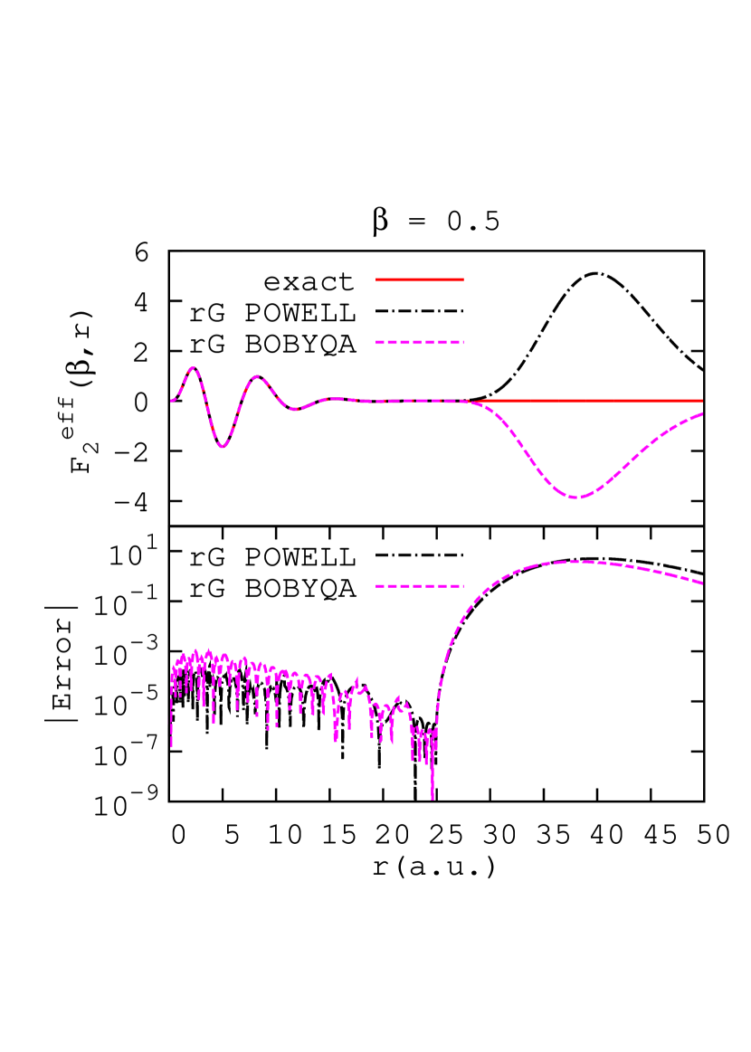
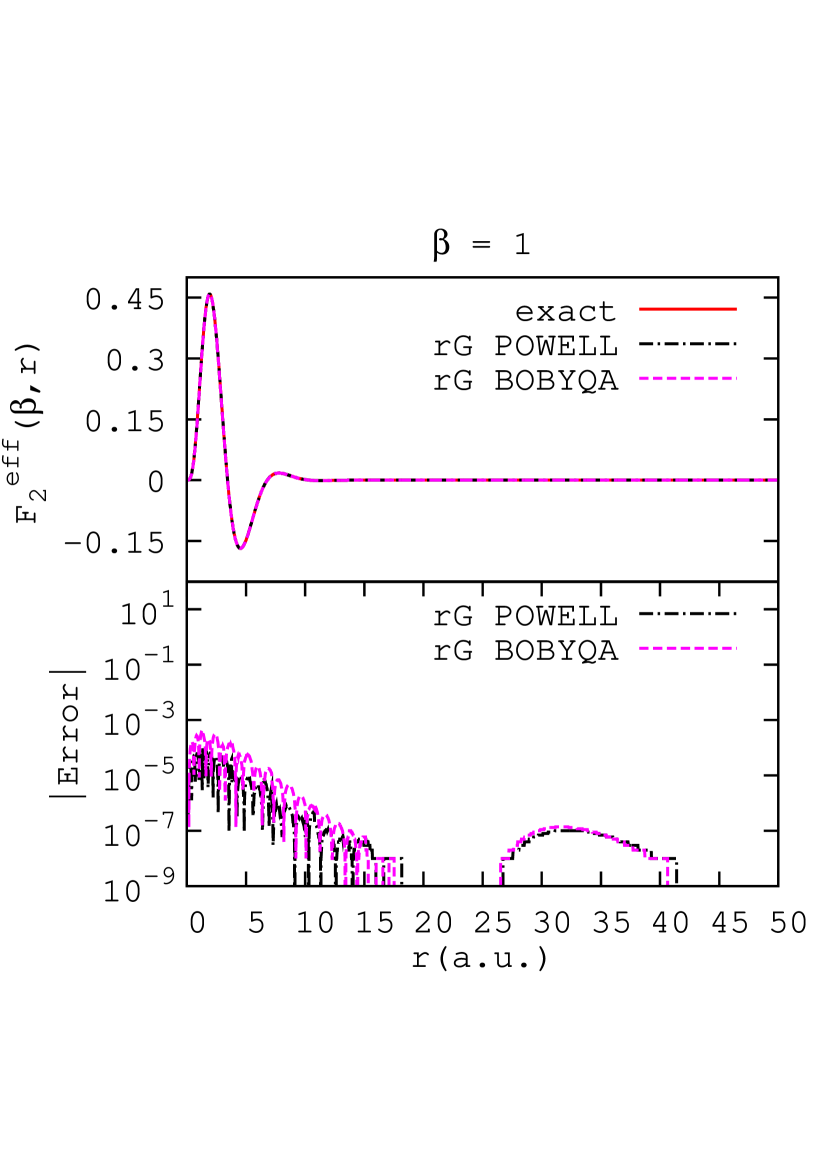
Figure 1: Effective function $F_{2}^{eff}(\beta,r)=F_{2}(r)e^{-\beta r}r^{2}$ ($l=1$ and $k_{2}=0.75~{}a.u.$) and its fitting with real Gaussians using Powell (rG POWELL) or BOBYQA (rG BOBYQA) optimizations, for $\beta=0.5$ (left upper panel) and $\beta=1$ (right upper panel). The absolute errors are plotted in the corresponding bottom panels.

the fitting of $F_{2}^{eff}(\beta,r)$ for two cases: $\beta=1$ and $\beta=0.5$, corresponding for example to the hydrogen $1s$ and $2s$ exponents, respectively. We clearly see that these fittings will cause trouble in the case $\beta=0.5$ since the deviation after $r=25$ will jeopardize radial integrals involving $F_{2}^{eff}(\beta,r)$. However when $\beta=1$ the bound state cancels this deviation. For higher energies ($\eta=3,\dots,6$) the same problem arises (not shown). The faster the functions oscillate the more important the deviation. For $\eta=1$, on the other hand, the decreasing term $e^{-\beta r}$ cancels this deviation for both $\beta=0.5$ and $\beta=1$.

2.2.3 Using reduced bounds (RB) for the search of the exponents

We try in this section to soften the errors coming from the diffused part of the fitting. To do so with BOBYQA, the optimization lower bound is modified to $\alpha_{min}=0.01$, so that $\alpha_{i}$ does not fall below $0.01$. The optimal set of exponents in this reduced bound (RB) case is shown in the fourth column of Table 1. They are overall of the same order of magnitude as those obtained without constraint but the lower bound forbids the smallest, possibly troublesome, exponents. Figure 2

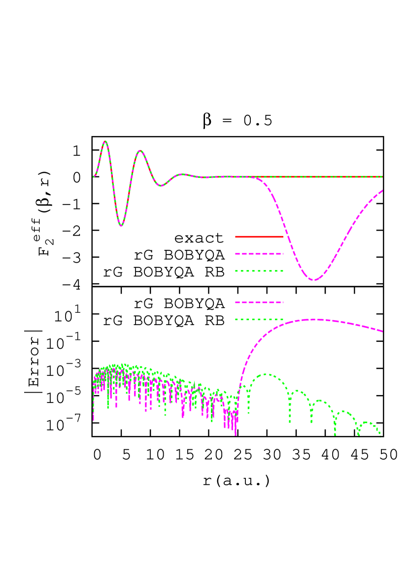
Figure 2: Upper panel: $F_{2}^{eff}=F_{2}(r)e^{-0.5r}r^{2}$ with its fitting using real Gaussians and BOBYQA without constraint on the exponents (rG BOBYQA) or after reducing the bounds (rG BOBYQA RB). The absolute error on the fitting is plotted in the bottom panel.

shows the resulting improvement at large distances of $F_{2}^{eff}$ (RB BOBYQA) in the case $\beta=0.5$. While the overall fitting is better, the accuracy is slightly worse in the fitting box $\mathscr{B}$ because imposing a constraint on the lower bound of $\alpha_{i}$ reduces the overall flexibility. Even in this RB approach the coefficients $\{c_{i}\}_{\eta}$ remain large. For example, the second column of Table 2 shows the magnitude of the coefficients $[c_{i}]_{5}$ for $\eta=5$ ($k_{5}=1.5$). All coefficients are larger than $10^{6}$ and most coefficients are of order $10^{10}$ or more. When the continuum functions are substituted by the Gaussian combinations, this ill-conditioning generates a numerical error that is related to the limited machine precision.

2.3 Complex Gaussians

In section 2.2 we have shown that representing oscillating functions with real Gaussians requires very small exponents $\{\alpha_{i}\}$ and implies very large coefficients $\{c_{i}\}$. This causes a large deviation out of the fitting box that may turn out to be troublesome in a given application. A partial solution could be to reduce the exponents bounds but the presence of very large values of $\{c_{i}\}$ does not disappear. We will now explore the ability of complex Gaussians to soften these problems.

In order to optimize the set $\mathscr{E}$ of functions (5) defined in section 2.1, we pick the initial complex exponents as:

$$\left\{\begin{aligned} &\ln(\Re(\alpha_{i}))=\frac{1}{N-1}\left[(N-i)\ln(a)+(i-1)\ln(b)\right]\\ &\Im(\alpha_{i})=0\end{aligned}\right.$$ (8)

with $a=10^{-4}$, $b=100$, and we fix the following research bounds:

$$\left\{\begin{aligned} &10^{-4}\leq\Re(\alpha_{i})\leq 1000\\ &-0.1\leq\Im(\alpha_{i})\leq 0.1\text{.}\end{aligned}\right.$$ (9)

The trust regions are $\Delta_{i}=0.01$ and $\Delta_{f}=10^{-6}$.

The optimal set of complex exponents obtained for the set $\mathscr{E}$ are shown in the fifth column of Table 1. We recall that the complex Gaussian expansion optimizes a set of real-valued radial Coulomb functions. Exponents do not appear in complex conjugate pairs, thus necessarily requiring complex coefficients to build up a real function. We verified that the imaginary part resulting from the complex combinations of the optimal complex Gaussians is indeed negligible.

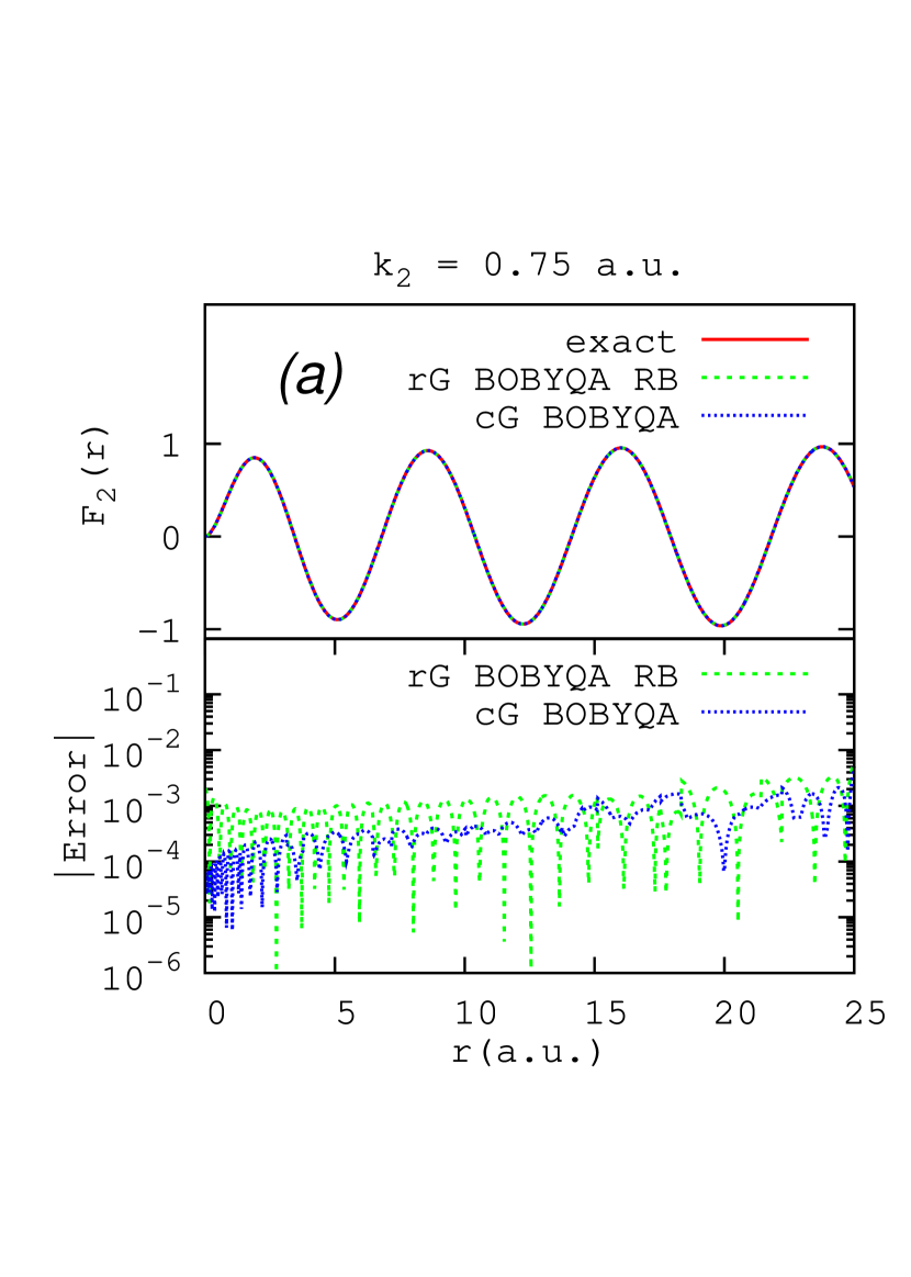
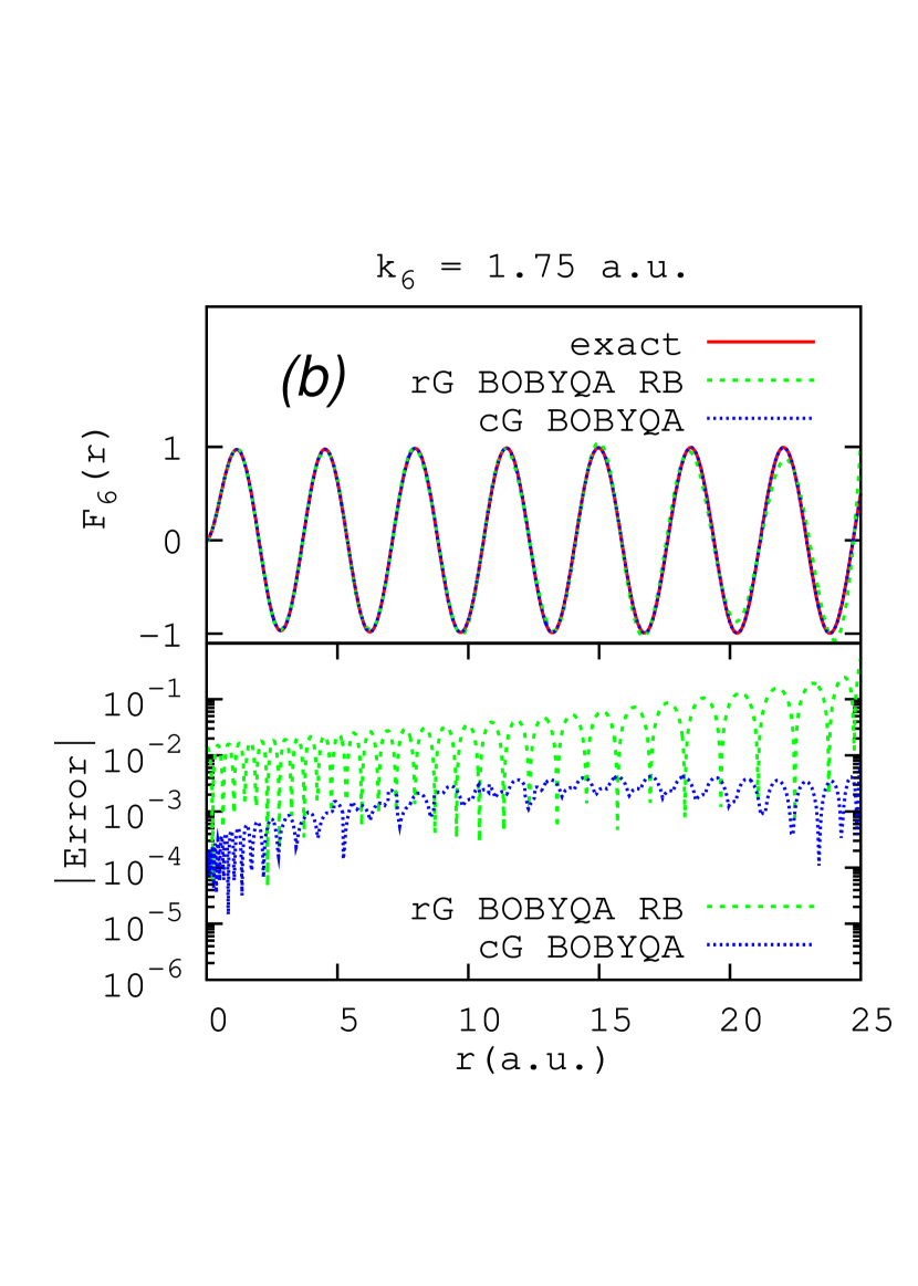
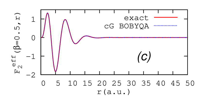
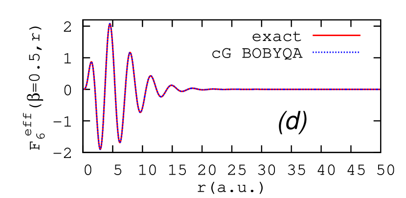
Figure 3: In panels (a) and (b) the sample Coulomb function $F_{\eta}(r)$, with $l=1$, is plotted for $\eta=2$ and $6$ respectively with the fitting by $30$ real Gaussians using BOBYQA with reduced bounds (rG BOBYQA RB) or by $30$ complex Gaussians (cG BOBYQA). The associated panels show the corresponding absolute errors within the fitting box. In the bottom panels (c) and (d) the effective function $F_{\eta}^{eff}(\beta,r)$ (see eq. (7)) with $\beta=0.5$ are compared to their cG BOBYQA representation, and this on a radial scale extended to $50~{}a.u.$.

Concerning the real part, Figure 3 shows two functions of the set, $F_{2}(r)$ and $F_{6}(r)$, with their fitting and the corresponding absolute errors, using: (i) $30$ real Gaussians and BOBYQA with constraints on $\{\alpha_{i}\}$ (rG BOBYQA RB) or (ii) $30$ complex Gaussians and BOBYQA (cG BOBYQA).

	rG POWELL	rG BOBYQA	rG BOBYQA RB	cG BOBYQA
$\alpha_{1}$	$0.0000092$	$0.0000128$	$0.0122973$	$0.0001000$ $+$ $0.0151526$ $j$
$\alpha_{2}$	$0.0000912$	$0.0000244$	$0.0145577$	$0.0001418$ $-$ $0.0171753$ $j$
$\alpha_{3}$	$0.0009435$	$0.0005575$	$0.0170202$	$0.0013875$ $-$ $0.0021493$ $j$
$\alpha_{4}$	$0.0019943$	$0.0016484$	$0.0197536$	$0.0019035$ $+$ $0.0216135$ $j$
$\alpha_{5}$	$0.0027596$	$0.0034884$	$0.0228103$	$0.0025827$ $+$ $0.0298661$ $j$
$\alpha_{6}$	$0.0044246$	$0.0084723$	$0.0262398$	$0.0034908$ $-$ $0.0241050$ $j$
$\alpha_{7}$	$0.0057793$	$0.0111337$	$0.0301176$	$0.0046754$ $-$ $0.0338441$ $j$
$\alpha_{8}$	$0.0072420$	$0.0136592$	$0.0344988$	$0.0061876$ $+$ $0.0378398$ $j$
$\alpha_{9}$	$0.0089783$	$0.0163089$	$0.0394645$	$0.0156781$ $+$ $0.0504851$ $j$
$\alpha_{10}$	$0.0114303$	$0.0194778$	$0.0451376$	$0.0196315$ $-$ $0.0395359$ $j$
$\alpha_{11}$	$0.0141988$	$0.0226689$	$0.0516205$	$0.0246020$ $-$ $0.0352098$ $j$
$\alpha_{12}$	$0.0178271$	$0.0267680$	$0.0591117$	$0.0308382$ $-$ $0.0302620$ $j$
$\alpha_{13}$	$0.0221354$	$0.0311299$	$0.0677411$	$0.0386508$ $-$ $0.0436192$ $j$
$\alpha_{14}$	$0.0272471$	$0.0358749$	$0.0778144$	$0.0484105$ $+$ $0.0624525$ $j$
$\alpha_{15}$	$0.0341612$	$0.0412564$	$0.0896070$	$0.0618203$ $+$ $0.0513264$ $j$
$\alpha_{16}$	$0.0436030$	$0.0473579$	$0.1036178$	$0.0816826$ $-$ $0.0552154$ $j$
$\alpha_{17}$	$0.0622928$	$0.0543047$	$0.1205385$	$0.1936246$ $+$ $0.0097332$ $j$
$\alpha_{18}$	$0.1058245$	$0.0616580$	$0.1407606$	$0.2915597$ $+$ $0.0024838$ $j$
$\alpha_{19}$	$0.1361998$	$0.0696498$	$0.1648189$	$0.4971406$ $-$ $0.0113366$ $j$
$\alpha_{20}$	$0.1729779$	$0.0779709$	$0.2204008$	$0.8532849$ $+$ $0.0200975$ $j$
$\alpha_{21}$	$0.2157985$	$0.0871103$	$0.2668776$	$1.3797714$ $+$ $0.0062079$ $j$
$\alpha_{22}$	$0.2755926$	$0.0970341$	$0.3164855$	$2.1958583$ $-$ $0.0311758$ $j$
$\alpha_{23}$	$0.3476818$	$0.1087089$	$0.3754007$	$3.5672935$ $-$ $0.0087858$ $j$
$\alpha_{24}$	$0.4425831$	$0.1228380$	$0.4395371$	$5.7419028$ $+$ $0.0012293$ $j$
$\alpha_{25}$	$0.6059363$	$0.1384401$	$0.5106744$	$9.2535835$ $-$ $0.0212019$ $j$
$\alpha_{26}$	$0.7983113$	$0.1591001$	$0.5897495$	$14.868739$ $-$ $0.0267870$ $j$
$\alpha_{27}$	$1.3120641$	$0.3614618$	$0.6853581$	$23.954872$ $-$ $0.0406721$ $j$
$\alpha_{28}$	$1.6592168$	$0.6148974$	$0.7913713$	$38.575864$ $+$ $0.0168896$ $j$
$\alpha_{29}$	$2.0833228$	$1.0857781$	$0.9151002$	$62.088037$ $-$ $0.0059998$ $j$
$\alpha_{30}$	$2.6339627$	$1.5257161$	$1.0660043$	$99.986651$ $+$ $0.0164035$ $j$

Table 1: Optimal exponents obtained after fitting the set $\mathscr{E}$ of Coulomb functions defined by eq. (5). rG POWELL means that the standard Powell method is used with real Gaussians, rG BOBYQA means that BOBYQA is used with real Gaussians, rG BOBYQA RB means that BOBYQA is used with reduced bounds of real exponents, and cG BOBYQA means that BOBYQA is used with complex Gaussians and coefficients.

It also shows the corresponding effective functions $F_{\eta}^{eff}(\beta,r)$, with no deviation due to the diffused Gaussians outside the box $\mathscr{B}$. One can clearly see that complex Gaussians reproduce the sample Coulomb functions with a better accuracy, and this becomes particularly evident for large energy values. The faster the functions oscillate, the more gainful complex Gaussians become. All expansion coefficients for the $F_{5}^{eff}$ case, shown in the third column of Table 2, remain moderate in contrast to the real Gaussian fitting.

	rG BOBYQA RB	cG BOBYQA
$c_{1}$	$+0.40823965E+07$	$-0.0767003$ $+$ $0.0491225$ $j$
$c_{2}$	$-0.55724942E+08$	$-0.0325026$ $+$ $0.1332674$ $j$
$c_{3}$	$+0.33793994E+09$	$+0.0134629$ $-$ $0.0432612$ $j$
$c_{4}$	$-0.11997914E+10$	$-0.0334812$ $+$ $0.5057190$ $j$
$c_{5}$	$+0.26244301E+10$	$+0.8455898$ $+$ $1.1476015$ $j$
$c_{6}$	$-0.28184368E+10$	$-1.4220978$ $+$ $0.5653343$ $j$
$c_{7}$	$-0.29542662E+10$	$-4.6750397$ $+$ $0.8996489$ $j$
$c_{8}$	$+0.20935337E+11$	$+3.1306684$ $-$ $2.6002539$ $j$
$c_{9}$	$-0.53704332E+11$	$-8.6221111$ $-$ $5.9017186$ $j$
$c_{10}$	$+0.95479441E+11$	$-12.3193333$ $-$ $198.5520668$ $j$
$c_{11}$	$-0.13228302E+12$	$-246.957659$ $+$ $276.197615$ $j$
$c_{12}$	$+0.15059598E+12$	$+131.906416$ $+$ $98.2360837$ $j$
$c_{13}$	$-0.14425237E+12$	$+148.629934$ $-$ $247.936566$ $j$
$c_{14}$	$+0.11764816E+12$	$-14.6173162$ $+$ $76.4157364$ $j$
$c_{15}$	$-0.82466268E+11$	$+12.0853088$ $-$ $104.198984$ $j$
$c_{16}$	$+0.49659844E+11$	$+18.8413901$ $+$ $99.0639125$ $j$
$c_{17}$	$-0.25966739E+11$	$-17.9257132$ $+$ $1.0993553$ $j$
$c_{18}$	$+0.11675152E+11$	$-6.9991082$ $+$ $8.5195011$ $j$
$c_{19}$	$-0.38808782E+10$	$-1.8509498$ $-$ $6.3255867$ $j$
$c_{20}$	$+0.12464857E+10$	$+0.9407901$ $+$ $5.5765830$ $j$
$c_{21}$	$-0.12293506E+10$	$-1.3594724$ $-$ $5.5649285$ $j$
$c_{22}$	$+0.10828614E+10$	$1.3522260$ $+$ $4.9085462$ $j$
$c_{23}$	$-0.84955303E+09$	$-1.5426203$ $-$ $4.0800303$ $j$
$c_{24}$	$+0.61321395E+09$	$+1.2864865$ $+$ $3.4277871$ $j$
$c_{25}$	$-0.36730844E+09$	$-1.0624354$ $-$ $2.7270828$ $j$
$c_{26}$	$+0.16987082E+09$	$+0.7979392$ $+$ $1.9979734$ $j$
$c_{27}$	$-0.57559060E+08$	$-0.5300813$ $-$ $1.2895942$ $j$
$c_{28}$	$+0.15043766E+08$	$+0.2829880$ $+$ $0.6875284$ $j$
$c_{29}$	$-0.24101691E+07$	$-0.1071319$ $-$ $0.2637591$ $j$
$c_{30}$	$+0.17331481E+06$	$+0.0207102$ $+$ $0.0528517$ $j$

Table 2: Optimal coefficients using BOBYQA to fit $F_{5}(r)$ with real Gaussians and reduced bounds (rG BOBYQA RB) and complex Gaussians (cG BOBYQA). Note that the number of digits shown here is not sufficient to rebuild the function in the case of (rG BOBYQA RB).

3 Illustrative applications to ionization problems

For illustration purposes, we consider hereafter a one-electron description. Computing ionization cross sections involves the calculation of transition matrix elements $T_{i\mathbf{k_{e}}}=\braket{\psi_{\mathbf{k_{e}}}^{-}(\mathbf{r})}{\widehat{O}}{\phi_{i}(\mathbf{r})}$ where $\phi_{i}(\mathbf{r})$ represents the initial (bound) wavefunction and $\psi_{\mathbf{k_{e}}}^{-}(\mathbf{r})$ represents the final (continuum) wavefunctions of the ejected electron (with momentum $\mathbf{k_{e}}$). In order to keep the present investigation free of extra numerical uncertainties and easily reproducible, we choose as continuum state the analytical Coulomb function

$$\psi_{\mathbf{k_{e}}}^{-}(\mathbf{r})=N(a)\frac{e^{i\mathbf{k_{e}}\mathbf{r}}}{(2\pi)^{\frac{3}{2}}}\mathstrut_{1}F_{1}\left(-ia,1;-i(k_{e}r+\mathbf{k_{e}}\mathbf{r})\right)\text{,}$$ (10)

where $N(a)=e^{\frac{\pi a}{2}}\Gamma(1+ia)$ with the Sommerfeld parameter $a=z/k_{e}$ and $z$ the charge seen by the ejected electron. $\widehat{O}$ is the transition operator that connects the initial to final states: $\frac{4\pi}{q^{2}}e^{i\mathbf{q}\cdot\mathbf{r}}$ in the case of particle impact ($\mathbf{q}$ is the momentum transfer vector) and $-\mathbf{\hat{\epsilon}}\cdot\mathbf{r}$ for photoionization in length gauge ($\mathbf{\hat{\epsilon}}$ is the polarization vector). In what follows, we will show that if the radial parts of both $\psi_{\mathbf{k_{e}}}^{-}$ and $\phi_{i}$ are expanded in Gaussians, the calculation of the transition matrix elements becomes analytical for both processes. As mentioned in the introduction the ultimate goal is to implement such an all-Gaussian approach to treat scattering from polyatomic molecules. Here, in order to illustrate the feasibility and the numerical robustness, we consider first an atomic case with an initial wavefunction given by:

$$\phi_{i}(\mathbf{r})=R_{n_{i}l_{i}}(r)Y_{l_{i}}^{m_{i}}(\hat{r})\text{,}$$ (11)

where $n_{i}$,$l_{i}$,$m_{i}$ are the usual quantum numbers. For the numerical illustration, we shall take as benchmark the hydrogen atom ($z=1$) for which exact cross sections are available and serve as a solid benchmark.

3.1 Hydrogen ionization by electron impact

We consider the ionization of a hydrogen atom by electron impact: $\text{e}^{-}+\text{H}\rightarrow\text{H}^{+}+2\text{e}^{-}$. In the first Born approximation the colliding electron is described by a plane wave before (momentum $\mathbf{k_{i}}$) and after the collision (momentum $\mathbf{k_{s}}$), while the wavefunction of the ejected electron is the Coulomb function $\psi_{\mathbf{k_{e}}}^{-}(\mathbf{r})$ of eq. (10). The cross section calculation involves the transition matrix element

$$T_{i\mathbf{k_{e}}}=\frac{4\pi}{q^{2}}F_{i\mathbf{k_{e}}}(\mathbf{q})\text{,}$$ (12)

where $\mathbf{q}=\mathbf{k_{i}}-\mathbf{k_{s}}$ is the momentum transfer vector and

$$F_{i\mathbf{k_{e}}}(\mathbf{q})=\braket{\psi_{\mathbf{k_{e}}}^{-}}{e^{i\mathbf{q}\mathbf{r}}}{\phi_{i}}$$ (13)

is the atomic form factor with $\phi_{i}$ the initial wavefunction (11).

The standard way to separate angular and radial variables is to use a partial wave expansion of the whole continuum wavefunction (10) over the spherical harmonics $Y_{l}^{m*}(\hat{r})Y_{l}^{m}(\hat{k_{e}})$:

$$\psi_{\mathbf{k_{e}}}^{-}(\mathbf{r})=\sqrt{\frac{2}{\pi}}\sum_{l,m}i^{l}e^{i\delta_{l}}\frac{F_{l,k_{e}}(r)}{kr}Y_{l}^{m*}(\hat{r})Y_{l}^{m}(\hat{k_{e}})\text{,}$$ (14)

where $F_{l,k_{e}}(r)$ is the regular radial Coulomb function (5) and $\delta_{l}=\text{arg}\left(\Gamma(l+1+\frac{zi}{k_{e}})\right)$ is the Coulomb phase shift. Alternatively, one can extract from the wavefunction (10) the highly oscillating behavior of the plane wave $e^{i\mathbf{k_{e}}\mathbf{r}}$ and expand in partial waves only the distortion factor represented by the confluent hypergeometric function. The hydrogen continuum state can then be written as

$$\psi_{\mathbf{k_{e}}}^{-}(\mathbf{r})=\frac{e^{i\mathbf{k_{e}}\mathbf{r}}}{(2\pi)^{\frac{3}{2}}}\sum_{l,m}D_{l,k_{e}}(r)Y_{l}^{m*}(\hat{r})Y_{l}^{m}(\hat{k_{e}})\text{,}$$ (15)

where the radial factors ³⁹

$$D_{l,k_{e}}(r)=4\pi e^{\frac{\pi}{2k_{e}}}\frac{\Gamma\left(1+\frac{i}{k_{e}}\right)\Gamma\left(l-\frac{i}{k_{e}}\right)(-i)^{l}}{\Gamma\left(-\frac{i}{k_{e}}\right)\Gamma(l+1)(2l+1)!!}(k_{e}r)^{l}\,\mathstrut_{1}F_{1}\left(l-\frac{i}{k_{e}},2l+2;-2ik_{e}r\right)$$ (16)

are complex functions. Fiori and Miraglia ²⁶ proposed to follow this second path and found that taking $l_{max}=8$ provides a sufficient accuracy in the calculation of hydrogen ionization by proton impact in a given energy range. If both $D_{l,k_{e}}(r)$ and the radial part of $\phi_{i}$ are represented by Gaussian combinations, then the transition matrix integral becomes analytical.

We should first shed light on the behavior of the radial $D_{l,k_{e}}(r)$ functions which, supposedly without strong oscillations ²⁶, should be easier to represent through a Gaussian set. Actually they are smooth only for low $l$. Functions with large values of $l$ manifest non negligible oscillations as illustrated by Figure 4

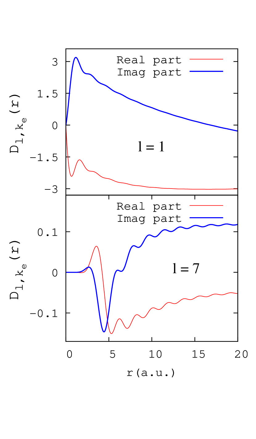
Figure 4: Real and imaginary parts of the $D_{l,k_{e}}(r)$ functions defined by eq. (16) for $k_{e}=1.75$ and $l=1$ (upper panel) or $l=7$ (lower panel).

which shows the behavior of $D_{1,k_{e}}(r)$ and $D_{7,k_{e}}(r)$ for $k_{e}=1.75$. While the small $l$ case can be easily represented with Gaussians, the oscillations of the large $l$ case result to be very difficult to reproduce. This $l$ dependence is even more pronounced for larger $k_{e}$ values. On the other hand, it is known that the first partial terms are generally those contributing the most to the continuum wavefunction. Consequently, the efficiency of the Gaussian fitting approach depends on the physical application under consideration and on the number of partial waves needed to achieve an overall acceptable accuracy.

To compare real and complex Gaussians, we use the strategy presented in section 2.1 for $9$ different sets of distortion functions, $\mathscr{D}_{l}:\{D_{l,{k_{e}}_{1}},D_{l,{k_{e}}_{2}},\dots,D_{l,{k_{e}}_{5}}\}$ for ${l=0,1,\dots,8}$. In each set we consider $5$ functions corresponding to ${k_{e}}_{\eta}=0.25+0.75(\eta-1)$. The fitting is performed up to $r=20$ and we set the parameter $g=18$ in eq. (3). Concerning the fitting with real Gaussians, for a given $l$ we optimize $\{\Re\left(D_{l,{k_{e}}_{1}}\right),\Re\left(D_{l,{k_{e}}_{2}}\right),\dots,\Re\left(D_{l,{k_{e}}_{5}}\right)\}$ using $20$ real Gaussians and $\{\Im\left(D_{l,{k_{e}}_{1}}\right),\Im\left(D_{l,{k_{e}}_{2}}\right),\dots,\Im\left(D_{l,{k_{e}}_{5}}\right)\}$ with $20$ other real Gaussians. On the other hand, in the complex case we use $20$ complex Gaussians to fit the set $\mathscr{D}_{l}$. In order to somehow take into account the $r^{l}$ behavior of $D_{l,k_{e}}(r)$ close to $r=0$, we add a $r^{\gamma_{l}}$ factor in the Gaussian expansion,

$$D_{l,k_{e}}(r)=r^{\gamma_{l}}\sum_{s}\left[c_{s}\right]_{l,k_{e}}\exp\left(-\left[\alpha_{s}\right]_{l}r^{2}\right)$$ (17)

where $\gamma_{0}=0$ and $\gamma_{l}=1$ for $l>0$. We use ${\gamma_{l}}=1$ instead of ${\gamma_{l}}=l$ as a compromise that gives the vanishing behavior close to $r=0$ for $l>0$ while avoiding error amplifications at large radial distances for large values of $l$. Figure 5

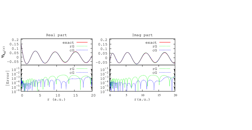
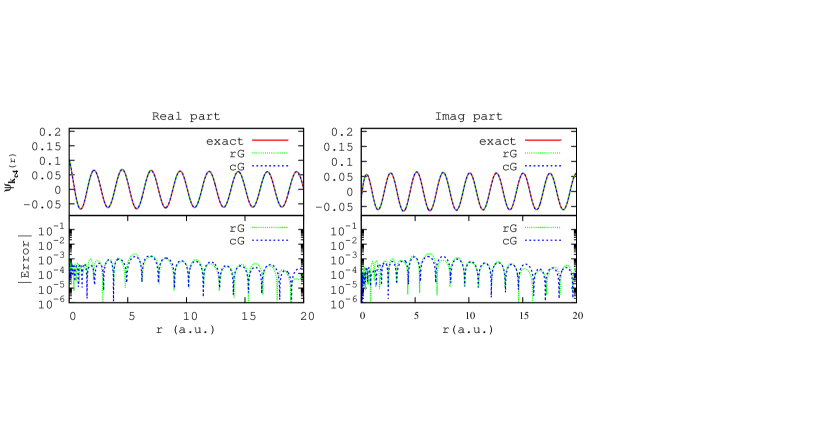
Figure 5: Real (left panels) and imaginary (right panels) part of the hydrogen continuum states $\psi_{\mathbf{k_{e}}}^{-}(\mathbf{r})$ calculated using eq. (15) with $l$ up to $l_{max}=8$ and comparison with that calculated by either real Gaussians (rG) or complex Gaussians (cG), for ${k_{e}}_{2}=1.00~{}a.u.$ (upper panels) and ${k_{e}}_{4}=2.50~{}a.u.$ (bottom panels), and $(\hat{r},\hat{k_{e}})=0$ in both cases. The corresponding absolute error on the fitting is shown in the bottom sub-panels.

shows the hydrogen continuum state at two energies ${k_{e}}_{2}=1$ and ${k_{e}}_{4}=2.5$, calculated using eq. (15) up to $l_{max}=8$, for an angle $(\hat{r},\hat{k_{e}})=0$, and with $D_{l,k_{e}}(r)$ represented by either real or complex Gaussians using eq. (17). The corresponding error on the fitting is also shown. For small energies the errors corresponding to the complex fitting are smaller. For large energies this advantage is lost since the partial waves with high order $l\gtrsim 3$ can not be reproduced accurately either by real or by complex Gaussians. Nevertheless the continuum wavefunction is overall well reproduced with both options because the first few terms $-$ which contribute the most to $\psi_{\mathbf{k_{e}}}^{-}$ $-$ are sufficiently well fitted. In summary, with expansion (15) the fitting difficulties due to oscillations are not completely removed as suggested in ²⁶ and we should remain aware of this weakness depending on the application. In the numerical illustration presented hereafter, the difficulty appears only in partial wave terms that do not contribute substantially and therefore do not affect the overall cross section calculation.

Let us now turn to the calculation of the atomic form factor (13) employing Gaussian expansion (17). The bound radial function of eq. (11) is also represented with either real or complex Gaussians:

$$R_{n_{i}l_{i}}(r)=\sum_{t}b_{t}e^{-\beta_{t}r^{2}}\text{.}$$ (18)

Using expansions (15), (17) and (18), the form factor becomes:

$$F_{i\mathbf{k_{e}}}(\mathbf{q})=\frac{1}{(2\pi)^{\frac{3}{2}}}\sum_{l,m}Y_{l}^{m*}(\hat{k_{e}})\sum_{s,t}\left[c_{s}\right]_{l,k_{e}}^{*}b_{t}\int d\mathbf{r}\,r^{\gamma_{l}}\,e^{i\mathbf{Q}\mathbf{r}}e^{-\left(\left[\alpha_{s}\right]_{l}^{*}+\beta_{t}\right)r^{2}}Y_{l_{i}}^{m_{i}}(\hat{r})Y_{l}^{m}(\hat{r})\text{,}$$ (19)

where $\mathbf{Q}=\mathbf{q}-\mathbf{k_{e}}$ is the momentum of the hydrogen ion after the collision. To separate angular and radial variables we use the Rayleigh expansion:

$$e^{i\mathbf{Q}\mathbf{r}}=4\pi\sum_{\lambda,\mu}i^{\lambda}j_{\lambda}(Qr)Y_{\lambda}^{\mu*}(\hat{Q})Y_{\lambda}^{\mu}(\hat{r})\text{,}$$ (20)

where $j_{\lambda}$ are the spherical Bessel functions. Therefore, in eq. (19) we have an integral over $3$ spherical harmonics multiplied by the following radial integral,

$$\mathcal{I}^{rad}=\int_{0}^{\infty}dr\,r^{2+\gamma_{l}}\,e^{-\left(\left[\alpha_{s}\right]_{l}^{*}+\beta_{t}\right)r^{2}}\,j_{\lambda}(Qr)$$ (21)

which can be calculated analytically (eq. $6.6.31$ of ⁴⁰):

$$\mathcal{I}^{rad}=\frac{\frac{\sqrt{\pi}}{4}\left(\frac{Q}{2}\right)^{\lambda}\Gamma\left(\frac{\lambda+\gamma_{l}+3}{2}\right)}{\Gamma\left(\lambda+\frac{3}{2}\right)}\left(\left[\alpha_{s}\right]_{l}^{*}+\beta_{t}\right)^{-\frac{\lambda+\gamma_{l}+3}{2}}\,\mathstrut_{1}F_{1}\left(\frac{\lambda+\gamma_{l}+3}{2},\lambda+\frac{3}{2};\frac{-Q^{2}}{4\left(\left[\alpha_{s}\right]_{l}^{*}+\beta_{t}\right)}\right)\text{.}$$ (22)

Finally the form factor (19) can be written as

$$F_{i\mathbf{k_{e}}}(\mathbf{q})=\sqrt{\frac{2l_{i}+1}{32\pi}}\sum_{l}\sqrt{2l+1}\sum_{\lambda=|l-l_{i}|}^{l+l_{i}}\frac{\left(\frac{iQ}{2}\right)^{\lambda}\Gamma\left(\frac{\lambda+\gamma_{l}+3}{2}\right)}{\Gamma\left(\lambda+\frac{3}{2}\right)}\sqrt{2\lambda+1}\mathscr{S}_{l,\lambda}^{rad}\mathscr{S}_{l,\lambda}^{ang}\text{,}$$ (23)

where

$$\mathscr{S}_{l,\lambda}^{rad}=\sum_{s,t}\left[c_{s}\right]_{l,k_{e}}^{*}b_{t}\left(\left[\alpha_{s}\right]_{l}^{*}+\beta_{t}\right)^{-\frac{\lambda+\gamma_{l}+3}{2}}\mathstrut_{1}F_{1}\left(\frac{\lambda+\gamma_{l}+3}{2},\lambda+\frac{3}{2};\frac{-Q^{2}}{4\left(\left[\alpha_{s}\right]_{l}^{*}+\beta_{t}\right)}\right)$$ (24)

and

$$\mathscr{S}_{l,\lambda}^{ang}=\begin{pmatrix}l&l_{i}&\lambda\\ 0&0&0\end{pmatrix}\sum_{m=-l}^{l}\begin{pmatrix}l&l_{i}&\lambda\\ m&m_{i}&-m-m_{i}\end{pmatrix}Y_{l}^{m*}(\hat{k_{e}})Y_{\lambda}^{-(m+m_{i})*}(\hat{Q})$$ (25)

where $\begin{pmatrix}j_{1}&j_{2}&j_{3}\\ m_{1}&m_{2}&m_{3}\end{pmatrix}$ denote the $3j$ Wigner coefficients. Assuming that the hydrogen target is in its ground state $1s$, it is possible to compare to the exact atomic factor ⁴¹:

$$F_{1s\mathbf{k_{e}}}(\mathbf{q})=\frac{2\sqrt{2}e^{\frac{\pi}{2k_{e}}}\Gamma\left(1-\frac{i}{k_{e}}\right)}{\pi(1+Q^{2})^{2}\mathsf{U}^{\frac{i}{k_{e}}}}\left[\left(1-\frac{i}{k_{e}}\right)+\frac{k_{e}+i}{k_{e}\mathsf{U}}\right]\text{,}$$ (26)

where

$$\mathsf{U}=\frac{q^{2}-(k_{e}+i)^{2}}{1+Q^{2}}\text{.}$$ (27)

The triple differential cross section (TDCS) is defined as:

$$\frac{d^{3}\sigma}{d\Omega_{s}d\Omega_{e}dE_{e}}=\frac{1}{4\pi^{2}}\frac{k_{s}k_{e}}{k_{i}}|T_{1s\mathbf{k_{e}}}(\mathbf{q})|^{2}\text{,}$$ (28)

with $E_{e}=k_{e}^{2}/2$ the energy of the ejected electron. $\Omega_{e}$ and $\Omega_{s}$ are the solid angles for the ejected and the scattered electron, respectively. We have calculated the TDCS for coplanar geometry at $E_{i}=k_{i}^{2}/2=250$ eV and scattering angle of $3^{\circ}$ for $k_{e}=0.25$, $1.00$ and $1.75$, with either real or complex Gaussian expansions. Both results, shown in Figure 6,

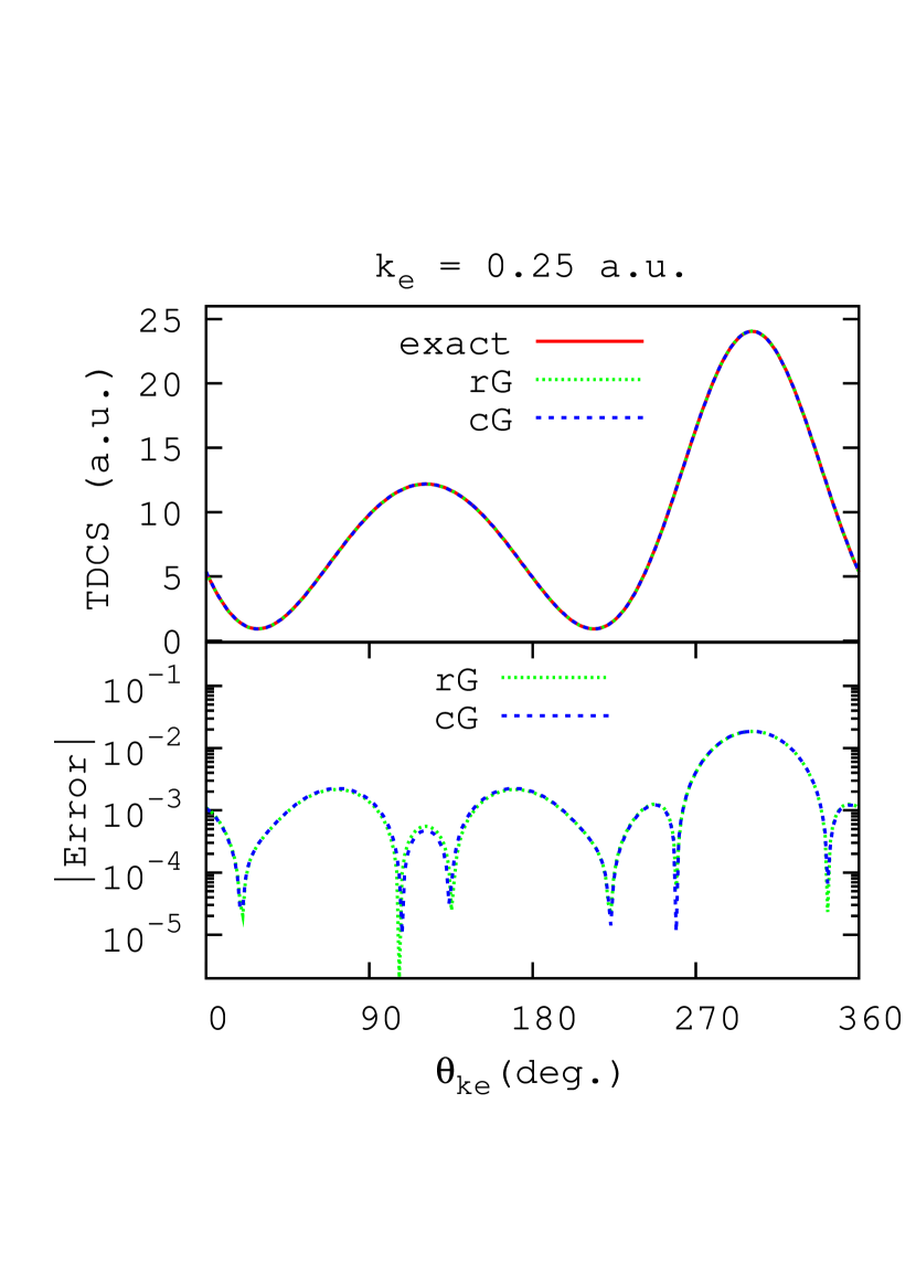
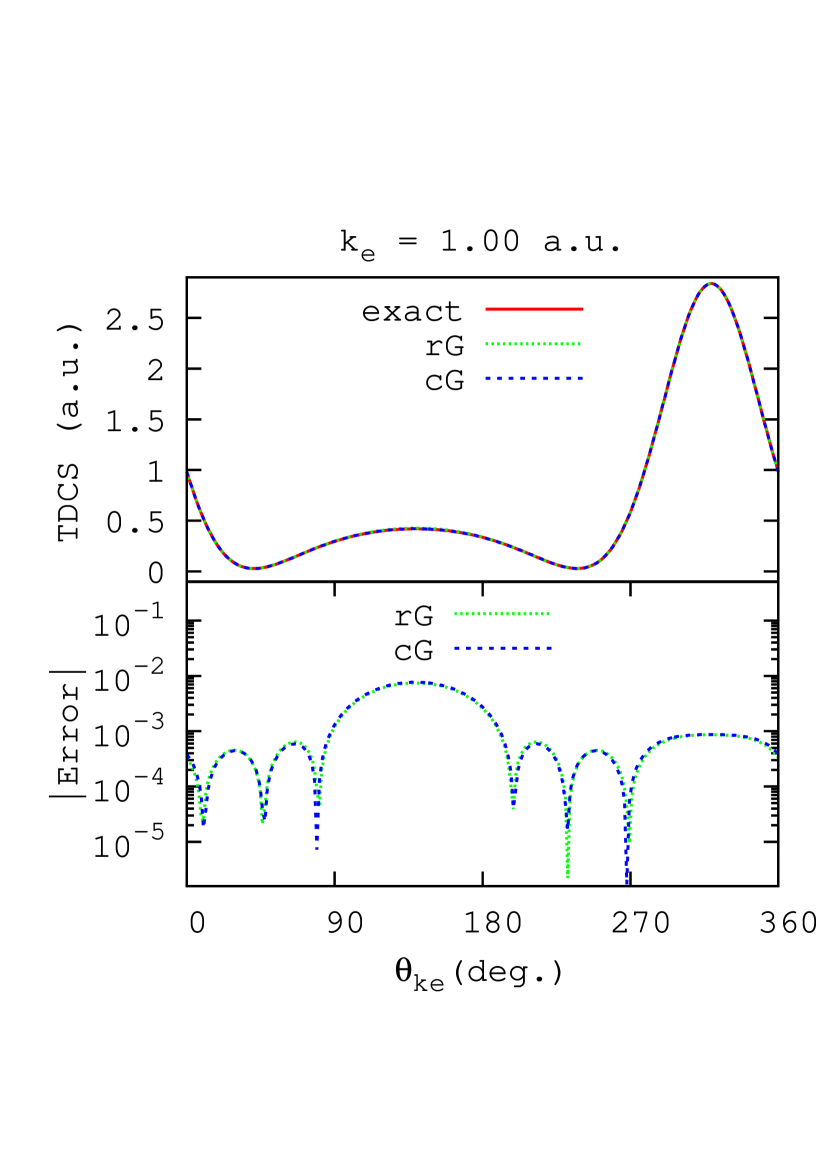
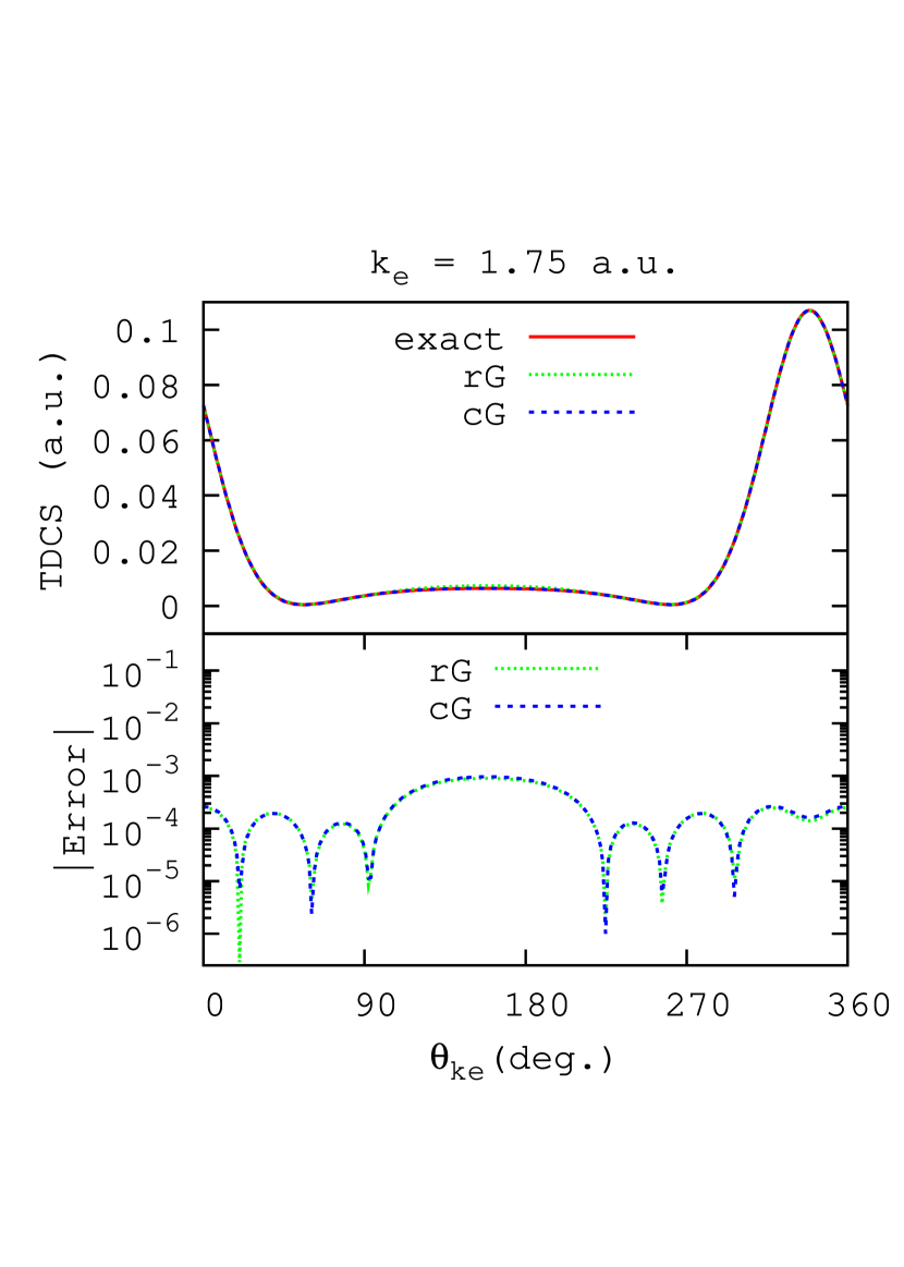
Figure 6: Upper panels: Triple differential cross section (TDCS) for the ionization of a hydrogen atom in the ground state by a $250$ eV electron, in coplanar geometry, with a scattering angle of $3^{\circ}$ and for ejected electron momentum $k_{e}=0.25$, $1.00$, or $1.75~{}a.u.$: Solid curves represent the exact analytical TDCS computed with eq. (26), and dotted/dashed curves represent the TDCS calculated with either real Gaussians (rG) or complex Gaussians (cG). The corresponding absolute error is shown in the bottom panels.

are very close to the exact values given by eq. (26), and display a similar accuracy. As discussed before, this can be related to the fact that the first partial functions $D_{l,k_{e}}(r)$ (making the largest contribution to the TDCS) are relatively smooth and can be well reproduced by both real and complex Gaussians with an equal precision. The very good reproduction of the exact cross section is also due to the presence of a fast decaying initial state ($e^{-r}$) so that any error from outside the fitting box will not affect the correct evaluation of the matrix element (see discussion in section 2).

Other scattering quantities can be tested. For example, by integrating over the solid angle of the scattered electron, one can define a doubly differential cross section (DDCS)

$$\frac{d^{2}\sigma}{dE_{e}d\Omega_{e}}=\int\frac{d^{3}\sigma}{d\Omega_{s}d\Omega_{e}dE_{e}}\,d\Omega_{s}.$$ (29)

The integration of the TDCS (28) is to be performed numerically from either the closed form of the form factor (Eq. (26) and (27)) or its partial expansion (Eq. (23), (24) and (25)) up to $l_{max}$ terms that make use of the Gaussian representation. As an illustration, in figure (7) we show the results as a function of the ejected energy $E_{e}=k_{e}^{2}/2$, for an incident energy $E_{i}=250$ eV, a coplanar geometry and the ejected angle fixed at $\theta_{e}=0$. We clearly observe that with $l_{max}=8$ in the continuum state representation, the expected cross section is recovered (with an error of less than 1 percent).

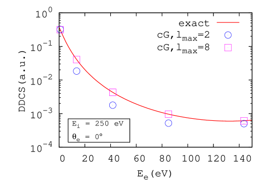
Figure 7: The doubly differential cross section (DDCS) with respect to the energy of the ejected electron, for an incident energy $E_{i}=250$ eV, a coplanar geometry and ejected angle $\theta_{e}=0$. The “exact” result (solid line) is obtained by integrating the TDCS (28) expressed using the closed form (Eq. (26) and (27)), while the cG results (symbols) are obtained by using the partial wave expansion (Eq. (23), (24) and (25)) and the complex Gaussian representation with $l_{max}=2$ or 8.

3.2 Photoionization

We now consider a hydrogen atom in the initial state $\phi_{i}$ illuminated by a photon of energy $E_{\gamma}=k_{e}^{2}/2+V_{\text{ion}}$, where $V_{\text{ion}}$ is the energy needed to ionize the target. This photon interacts with the atom leading to an ion and a photo-electron of energy $E_{k_{e}}=k_{e}^{2}/2$. The photoionization cross section is defined as ⁴²

$$\sigma=\frac{4\pi^{2}k_{e}E_{\gamma}}{c}\frac{1}{2l_{i}+1}\sum_{m_{i}}\int d\Omega_{\mathbf{k_{e}}}\,\left|T_{i\mathbf{k_{e}}}\right|^{2}\text{,}$$ (30)

where $c$ is the speed of light in vacuum and $\Omega_{\mathbf{k_{e}}}$ is the solid angle of the ejected photo-electron. In the length gauge and the dipole approximation the transition matrix element is given by

$$T_{i\mathbf{k_{e}}}=\langle\psi_{\mathbf{k_{e}}}^{-}(\mathbf{r})|-\hat{\epsilon}\cdot\mathbf{r}|\phi_{i}(\mathbf{r})\rangle\text{,}$$ (31)

where $\hat{\epsilon}$ defines the polarization direction. Here we expand the hydrogen continuum wavefunction (10) in the standard way; expansion (14) presents the advantage that selection rules reduce the summation over $l$ to just $l=l_{i}-1$ and $l=l_{i}+1$. In contrast, when using expansion (15), converged photoionization calculations require many partial terms in order to cover large physical distances. For example we found that for a $1s$ hydrogen target, about $10$ partial terms $D_{l,k_{e}}(r)$ are needed to achieve a relative error of the order $0.01$, and one has to consider $\approx 30$ partial terms to reach a similar accuracy if the hydrogen is initially in the radially more extended $2s$ state. With expansion (14), only two partial terms appear in both $1s$ and $2s$ cases.

The calculation of transition matrix elements (31) involves two integrals:

$$\mathscr{J}^{ang}=\int\ Y_{l}^{m*}(\hat{r})Y_{1}^{0}(\hat{r})Y_{l_{i}}^{m_{i}}(\hat{r})d\Omega_{\mathbf{r}}\text{,}$$ (32)

and

$$\mathscr{J}_{l}^{rad}=\int_{0}^{\infty}\,F_{l,k_{e}}(r)\,R_{n_{i}l_{i}}(r)\,r^{2}\,dr\text{.}$$ (33)

The angular integral $\mathscr{J}^{ang}$ imposes the selection rules $l=l_{i}\pm 1$ and $m=m_{i}$. The radial function $R_{n_{i}l_{i}}(r)$ is fitted by real Gaussians as in eq. (18), and the functions $F_{l,k_{e}}(r)$ are written as

$$F_{l_{i}\pm 1,k_{e}}(r)=\sum_{s}\left[c_{s}\right]_{l_{i}\pm 1,k_{e}}\exp(-[\alpha_{s}]_{l_{i}\pm 1}r^{2})\text{.}$$ (34)

with the different Gaussian parameters optimized to fit the $\mathscr{E}$ set, given in Table 1. Using these Gaussian representations, the radial integral becomes

$$\mathscr{J}_{l_{i}\pm 1}^{rad} =\frac{\sqrt{\pi}}{4}\sum_{s,t}\left[c_{s}\right]_{l_{i}\pm 1,k_{e}}b_{t}{\left([\alpha_{s}]_{l_{i}\pm 1}+\beta_{t}\right)}^{-\frac{3}{2}}\text{.}$$ (35)

After summation over the magnetic numbers $m_{i}$, the cross section can be simply expressed as:

$$\sigma=\frac{8\pi\,E_{\gamma}}{3\,(2l_{i}+1)\,k_{e}\,c}\Bigg{[}l_{i}\left(\mathscr{J}_{l_{i}-1}^{rad}\right)^{2}+(l_{i}+1)\left(\mathscr{J}_{l_{i}+1}^{rad}\right)^{2}\Bigg{]}$$ (36)

For a hydrogen target initially in a $ns$ state the cross section calculation involves only the $l=1$ partial function (5) which is expanded using the different Gaussian sets optimized to fit the $\mathscr{E}$ set given in section 2.

Figure 8

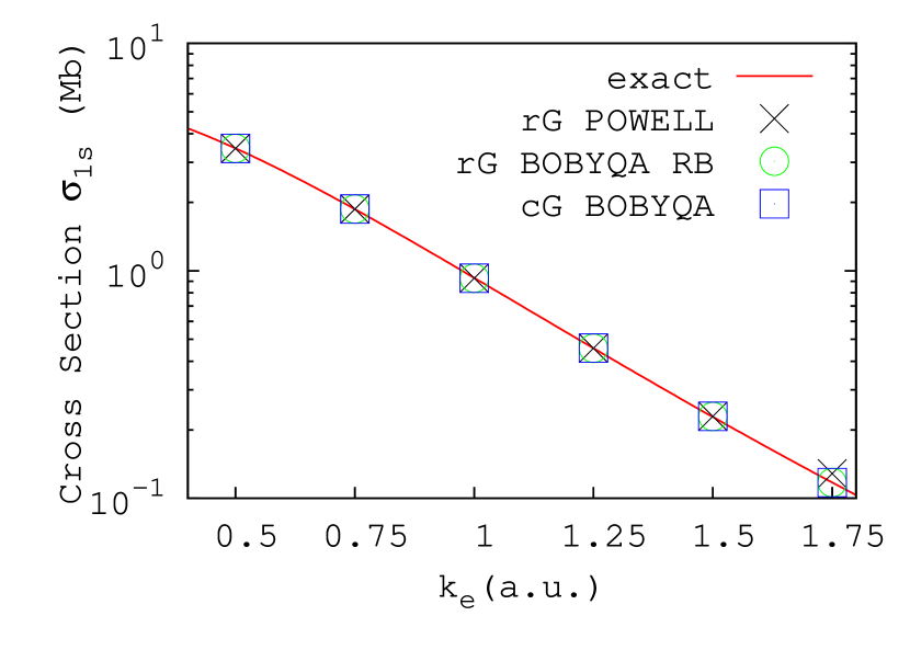
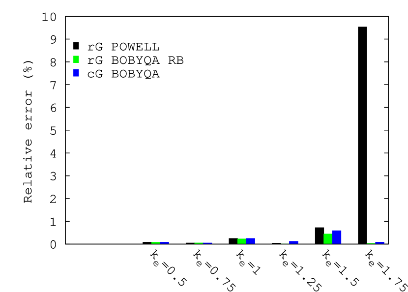
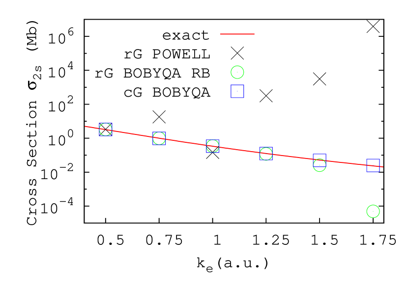
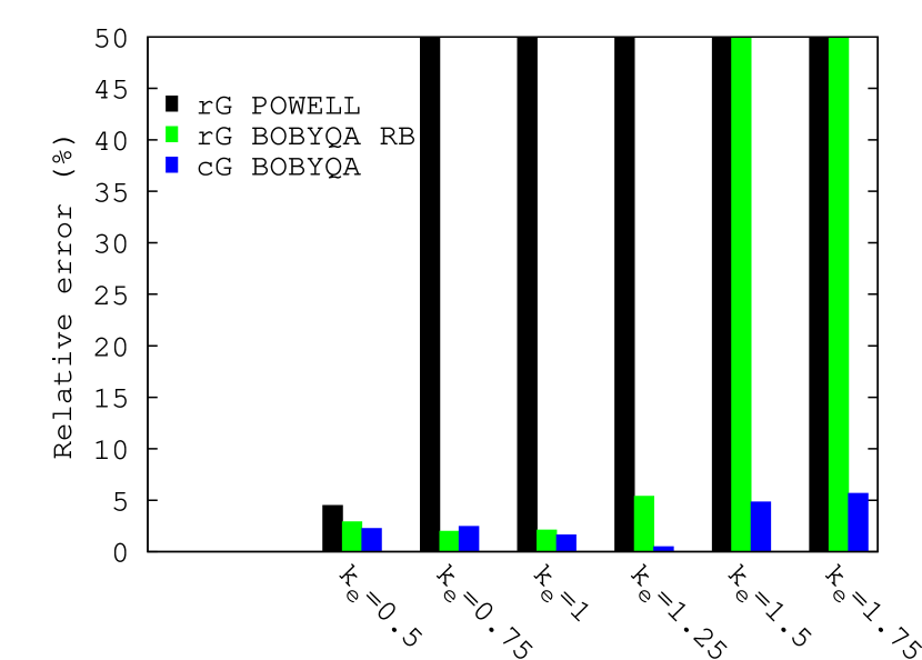
Figure 8: Hydrogen photo-ionization cross section (in Mb) in terms of photo-electron wavenumber (in $a.u.$). The hydrogen atom is initially in the $1s$ state (upper panels), and in the $2s$ state (bottom panels). Black crosses, green circles and blue squares refer respectively to cross sections computed with real Gaussians with Powell, real Gaussians with BOBYQA by imposing reduced bounds, and complex Gaussians with BOBYQA. On the right panels, the histograms show the corresponding relative errors on the cross section computed with Gaussians.

shows the photoionization cross section as a function of the photo-electron wavenumber $k_{e}$ for initial states $1s$ or $2s$, calculated with real Gaussians optimized using Powell (rG POWELL), real Gaussians optimized using BOBYQA with reduced bounds (rG BOBYQA RB), complex Gaussians optimized using BOBYQA (cG BOBYQA) and the exact results given by ⁴³:

$$\sigma_{1s}=\frac{2^{5}\pi^{2}e^{-4\frac{\arctan(k_{e})}{k_{e}}}}{3cE_{\gamma}^{4}\left(1-e^{-2\frac{\pi}{k_{e}}}\right)}\text{,}$$ (37)

and

$$\sigma_{2s}=\frac{\pi^{2}\left(8+\frac{3}{E_{\gamma}}\right)e^{-4\frac{\arctan(2k_{e})}{k_{e}}}}{6cE_{\gamma}^{4}\left(1-e^{-2\frac{\pi}{k_{e}}}\right)}\text{.}$$ (38)

The corresponding relative errors are plotted in a histogram. The results are consistent with the quality of the fitting detailed in section 2. Concerning H($1s$), there is no important difference between the different Gaussian basis sets except for the largest energy, $k_{e}=1.75$ where the rG POWELL method fails. As explained in section 2, this is due to large deviations outside the fitting box. For H($2s$) the calculation with rG POWELL completely fails except for the small energy case $k_{e}=0.50$. The calculation with rG BOBYQA RB gives a small relative error at low energies, but fails above $k_{e}=1.25$. Only the cG BOBYQA choice achieves a very good accuracy in both $1s$ and $2s$ cases for all energies. These photoionisation cross section calculations demonstrate that care must be taken when using Gaussian expansions for continuum states, especially at higher energies and if they appear in matrix elements whose integrands extend on a large radial domain. For these delicate cases, complex Gaussians are clearly superior to their real counterpart.

4 Conclusions

In this work we applied a full nonlinear optimization to represent oscillating functions with both real and complex Gaussians by using a least square approach in combination with a quadratic approximation method. We have shown that real Gaussians may be sufficient to correctly span the space of functions within the fitting box, however they behave erroneously outside with sometimes very large errors due to diverging coefficients. Real Gaussian representation of continuum radial functions can nevertheless be used in ionization integrals if the decay factor associated with the bound state decreases fast enough to compensate this weakness. This may not be the case for highly excited states. Imposing a constraint on the Gaussian exponents reduces the error magnitude at small energies but it also reduces the fitting accuracy in the box and does not resolve the problem of ill-conditioned coefficients. On the other hand, complex Gaussians have an intrinsically oscillating behavior and are clearly more appropriate to fit bound functions that spread over large distances (highly excited or Rydberg states) and scattering functions.

As an illustrative application, we have used the regular Coulomb wavefunctions fitted by Gaussians in hydrogen ionization problems. The accuracy of cross sections reproduced with complex Gaussians is as good as that obtained with real Gaussians at small energies while it is clearly superior at large energies, where real Gaussians fail completely. The application also allowed us to show the advantage provided by an all-Gaussian approach: the matrix elements can be evaluated analytically once all involved functions, bound and continuum, are expanded in real or complex Gaussians. In the present work we considered pure Coulomb continuum functions but our numerical strategy can be applied in the same manner to any one-center distorted wavefunctions generated analytically or numerically. We have already successfully tested the complex Gaussian representation of positive energy generalized Sturmian functions ⁴⁴; with an adequately chosen asymptotic behavior, the latter can be used as an efficient basis to expand any distorted wave and thus to study collision problems.

Extension to more complicated situations, including many-electron atoms and those molecules that can be described successfully with one-center expansions, do not present any additional technical difficulties. Going beyond scattering from a central potential, electron-electron integrals can be treated within a multipolar approach, and dealing with the ensuing integrals is part of our current investigations. Work is also ongoing to extend our proposal to study ionization processes with molecular targets, and thus to deal with multicenter integrals. For molecules the initial electronic wavefunctions are often already calculated in Gaussian bases. The representation of continuum states by Gaussians, even with complex exponents, should provide a way to simplify some of the multidimensional numerical integrations needed in scattering calculations. The use of the Gaussian product theorem will lead to some meaningless complex centers. These, however, do not lead to mathematical obstacles that cannot be dealt with as indicated in the work of Kuang and Lin ^{34, 35}.

References

- [1] Boys, S. F. Proc. R. Soc. London, Ser. A 1950, 200, 542-554.
- [2] Hill, J. G. Int. J. Quantum Chem. 2013, 113, 21-34.
- [3] Reeves, C. M., Harrison, M. C. J. Chem. Phys. 1963, 39, 11-17.
- [4] Feller, D. F., Ruedenberg, K. Theor. Chim. acta 1979, 52, 231-251.
- [5] Huzinaga, S., Klobukowski, M. Chem. Phys. Lett. 1985, 120, 509-512.
- [6] Alexander, S. A., Monkhorst, H. J., Szalewicz, K. J. Chem. Phys. 1986, 85, 5821-5825.
- [7] Petersson, G. A., Zhong, S., Montgomery, J. A., Frisch, M. J. J. Chem. Phys. 2003, 118, 1101-1109.
- [8] Huzinaga, S. J. Chem. Phys. 1965, 42, 1293-1302.
- [9] Reeves, C. M., Fletcher, R. J. Chem. Phys. 1965, 42, 4073-4081.
- [10] O-ohata, K., Taketa, H., Huzinaga, S. J. Phys. Soc. Jpn. 1966, 21, 2306-2324.
- [11] Lim, T. K., Whitehead, M. A. J. Chem. Phys. 1966, 45, 4400-4413.
- [12] Stewart, R. F. J. Chem. Phys. 1969, 50, 2485-2495.
- [13] Stewart, R. F. J. Chem. Phys. 1970, 52, 431-438.
- [14] Harris, F. E. Rev. Mod. Phys. 1963, 35, 558-568.
- [15] Marante, C., Argenti, L., Martín, F. Phys. Rev. A 2014, 90, 012506.
- [16] Cacelli, I., Moccia, R., Rizzo, A. J. Chem. Phys. 1993, 98, 8742-8748.
- [17] Cacelli, I., Moccia, R., Rizzo, A. J. Chem. Phys. 1995, 102, 7131-7141.
- [18] Cacelli, I., Moccia, R., Rizzo, A. J. Chem. Phys. 1998, 57, 1895-1905.
- [19] Coccia, E., Mussard, B., Labeye, M., Caillat, J., Taïeb, R., Toulouse, J., Luppi, E. Int. J. Quantum Chem. 2016, 116, 1120-1131.
- [20] Coccia, E., Luppi, E. Theor. Chem. Acc. 2016, 135, 43.
- [21] Coccia, E., Assaraf, R., Luppi, E., Toulouse, J. J. Chem. Phys. 2017, 147, 014106.
- [22] Tennyson, J. Phys. Rep. 2010, 491, 29-76.
- [23] Kaufmann, K., Baumeister, W., Jungen, M. J. Phys. B - At. Mol. Opt. 1989, 22, 2223-2240.
- [24] Nestmann, B. M., Peyerimhoff, S. D. J. Phys. B - At. Mol. Opt. 1990, 23, 773-777.
- [25] Faure, A., Gorfinkiel, J. D., Morgan, L. A., Tennyson, J. Comput. Phys. Commun. 2002, 144, 224-241.
- [26] Fiori, M., Miraglia, J. E. Comput. Phys. Commun. 2012, 183, 2528-2534.
- [27] McCurdy Jr, C. W., Rescigno, T. N. Phys. Rev. Lett. 1978, 41, 1364-1368.
- [28] McCurdy, C. William, Mowrey, Richard C. Phys. Rev. A 1982, 25, 2529-2538.
- [29] Isaacson, A. D. J. Chem. Phys. 1991, 94, 388-396.
- [30] White, A. F., Epifanovsky, E., McCurdy, C. W., Head-Gordon, M. J. Chem. Phys. 2017, 146, 234107.
- [31] Matsuzaki, R., Yabushita, S. J. Comput. Chem. 2017, 38, 910-925.
- [32] Matsuzaki, R., Yabushita, S. J. Comput. Chem. 2017, 38, 2030-2040.
- [33] Matsuzaki, R., Asai, S., McCurdy, C. W., Yabushita, S. Theor. Chem. Acc. 2014, 133, 1-12.
- [34] Kuang, J., Lin, C. D. J. Phys. B. : At. Mol. Opt. Phys. 1997, 30, 2529-2548.
- [35] Kuang, J., Lin, C. D. J. Phys. B. : At. Mol. Opt. Phys. 1997, 30, 2549-2567.
- [36] Powell, M. J. D. Comput. J. 1964, 7, 155-162.
- [37] Powell, M. J. D., Technical Report No. DAMTP 2009/NA06, Centre for Mathematical Sciences, University of Cambridge, UK, 2009. The subroutine is available on https://www.zhangzk.net/ and https://www.pdfo.net/
- [38] Abramowitz, M., Stegun, I., Eds; Handbook of Mathematical Functions; Dover, New York, 1964; Chapter 14, p 538.
- [39] Spielberger, L., Bräuning, H., Muthig, A., Tang, J. Z., Wang, J., Qiu, Y., Dörner, R., Jagutzki, O., Tschentscher, Th., Honkimäki, V., Mergel, V., Achler, M., Weber, Th., Khayyat, Kh., Burgdörfer, J., McGuire, J., Schmidt-Böcking, H. Phys. Rev. A 1999, 59, 371-379.
- [40] Gradshteyn, I. S., Ryzhik, I. M., Eds; Table of Integrals, Series, and Products; Academic Press, New York, 2007; Chapter 6, p 706.
- [41] McDowell, M. R. C., Coleman J. P., Eds; Introduction to the Theory of Ion-Atom collisions; North-Holland, New York, 1970; Chapter 7, pp 322-324.
- [42] Burke, P. G.; R-Matrix Theory of Atomic Collisions; Springer, Berlin, 2011; Chapter 8, pp 380-390.
- [43] Harriman, J. M. Phys. Rev. 1956, 101, 594-598.
- [44] Gasaneo, G., Ancarani, L. U., Mitnik, D. M., Randazzo, J. M., Frapiccini, A. L., Colavecchia, F. D. Adv. Quantum Chem. 2013, 67, 153-216.