Searching for primordial helical magnetic fields

Abstract

The presence of non-zero helicity in intergalactic magnetic fields (IGMF) has been suggested as a clear signature for their primordial origin. We extend a previous analysis of diffuse Fermi-LAT gamma-ray data from 2.5 to more than 11 years and show that a hint for helical magnetic fields in the 2.5 year data was a statistical fluctuation. Then we examine the detection prospects of helical magnetic fields using individual sources as, e.g., TeV gamma-ray blazars. We find that a detection is challenging employing realistic models for the cascade evolution, the IGMF and the detector resolution in our simulations.

I Introduction

Magnetic fields are known to play a prominent role for the dynamics and in the energy budget of astrophysical systems on galactic and smaller scales, but their role on larger scales is still elusive Kulsrud and Zweibel (2008); Durrer and Neronov (2013). So far, only in a few galaxy clusters observational constraints have been obtained, either by detecting their synchrotron radiation halos or by performing Faraday rotation measurements. Since both observational methods need a prerequisite to measure magnetic fields (a high thermal density for rotation measurements and the presence of relativistic particles for radio emission), they have been successfully applied only to high density regions of collapsed objects as galaxies and galaxy clusters. Fields significantly below the $\mu$G level are barely detectable with these methods. Also other constraints, for instance the absence of distortions in the spectrum and the polarization properties of the cosmic microwave background radiation, imply only a fairly large, global upper limit on the intergalactic magnetic field (IGMF) at the level of $10^{-9}$ G.

An alternative approach to obtain information about the IGMF is to use its effect on the radiation from TeV gamma-ray sources. The multi-TeV gamma-ray flux from distant blazars is strongly attenuated by pair production on the infrared/optical extragalactic background light (EBL), initiating electromagnetic cascades in the intergalactic space Nikishov (1961); Gould and Schréder (1966); Berezinsky and Smirnov (1975); Strong (1976). The charged component of these cascades is deflected by the IGMF. Potentially observable effects of such electromagnetic cascades in the IGMF include the delayed “echoes” of multi-TeV gamma-ray  flares or gamma-ray bursts Plaga (1995); Takahashi et al. (2008); Murase et al. (2008), the appearance of extended emission around initially point-like gamma-ray sources Aharonian et al. (1994); Neronov and Semikoz (2007); Dolag et al. (2009); Elyiv et al. (2009); Neronov et al. (2010), and the suppression of GeV halos around TeV blazars d’Avezac et al. (2007). The last method has been used to derive lower limits on the strength and the filling factor of the IGMF Neronov and Vovk (2010); Tavecchio et al. (2010); Dolag et al. (2011). However, it is unclear if plasma instabilities invalidate these claims, as argued first in Ref. Broderick et al. (2012).

The observed magnetic fields in galaxies and galaxy clusters are assumed to result from the amplification of much weaker seed fields. Such seeds could be created in the early universe, e.g. during phase transitions or inflation, and then amplified by plasma processes Durrer and Neronov (2013). If the generation mechanism of such primordial fields, as e.g. sphalerons in the electroweak sector of the standard model, breaks CP then the IGMF will have a non-zero helicity. In the case of helical fields an “inverse cascade” may transfer power from smaller to larger length scales Brandenburg et al. (1996); Olesen (1997), increasing thereby its observable effects. Moreover, helical fields decay slower than non-helical ones. Therefore a small non-zero initial helicity fraction is increasing with time, making the field either completely left- or right-helical today. A clean signature for a primordial origin of the IGMF is therefore its non-zero helicity. In a series of works, Vachaspati and collaborators worked out possible observational consequences of a helical IGMF Tashiro and Vachaspati (2013); Tashiro et al. (2014); Tashiro and Vachaspati (2015); Long and Vachaspati (2015). Moreover, they examined gamma-ray data from the Fermi-LAT satellite and found a 2.5 $\sigma$ hint for the presence of a helical IGMF Tashiro et al. (2014); Chen et al. (2015).

In this work, we re-analyze the gamma-ray data from Fermi-LAT in Sec. II, extending the data set from 2.5 years used in Ref. Chen et al. (2015) to more than 11 years. We find that this data set composed of diffuse gamma-rays is consistent with zero helicity. This result is expected for a diffuse photon flux, because the contributions from positive and negative charges in an electromagnetic cascade cancel in observables sensitive to non-zero helicity. Thus a possible signal for helical magnetic fields is suppressed in the diffuse flux, since the number of sources per considered angular patch on the sky is typically large. In Sec. III, we examine therefore the detection prospects of non-zero helicity in the IGMF using individual sources as, e.g., blazars. If such a source is seen from the side, preferentially one charge may be deflected towards the observer. Such a charge separation may in turn render the detection of helicity possible. Starting from a toy model similar to the one in Ref. Long and Vachaspati (2015), we investigate how strong the addition of realistic features like fluctuations in the interaction length and the IGMF as well as experimental errors deteriorates the detection prospects. We summarize our conclusions in Sec. IV.

II Diffuse gamma-rays from 10+ years of Fermi data

The authors of Ref. Tashiro and Vachaspati (2015) suggested to use as observable $Q$ to detect a helical IGMF the triple scalar product of the arrival directions $\boldsymbol{n}_{i}$ (normalized as $|\boldsymbol{n}_{i}|=1$) of three photons from the diffuse gamma-ray background. Depending on their energies $\varepsilon_{i}$, photons are split into three different energy bins with lower bounds $E_{3}$, $E_{2}$, and $E_{1}$. Each bin has a size $\Delta E$, given by dividing the range of photon energies by the number of bins. Photons are binned such that $E_{i}<\varepsilon_{i}<E_{1}+\Delta E$ for $i=\{1,2,3\}$. Photons outside these energy ranges are discarded. The arrival directions of the photons in the highest energy bin, i.e. those with $E_{3}<\varepsilon_{3}<E_{3}+\Delta E$, serve as proxy for the direction to potential sources, since such secondary photons are typically produced by cascade electrons with higher energies which are in turn less deflected. If all three photons originate from the same source, a curve connecting the highest energy photon to the lowest energy photons in decreasing order will be bent to the right in a right-handed helical magnetic field. Similarly, the triple scalar product $(\boldsymbol{n}_{1}\times\boldsymbol{n}_{2})\cdot\boldsymbol{n}_{3}$ will be positive, while it will be negative for a left-handed helical field. The estimator $Q$ is thus defined as Tashiro and Vachaspati (2015)

$$Q= \frac{1}{N_{1}N_{2}N_{3}}\sum_{i,j,k}(\boldsymbol{n}_{i}(\varepsilon_{1})\times\boldsymbol{n}_{j}(\varepsilon_{2}))\cdot\boldsymbol{n}_{k}(\varepsilon_{3})$$

$$W_{R}(\boldsymbol{n}_{i}(\varepsilon_{1})\cdot\boldsymbol{n}_{k}(\varepsilon_{3}))W_{R}(\boldsymbol{n}_{j}(\varepsilon_{2})\cdot\boldsymbol{n}_{k}(\varepsilon_{3})),$$ (1)

where $N_{i}$ denotes the number of photon in the bin $i$ and $W_{R}$ a top-hat window function. Its radius $R$ is a free parameter introduced to ensure that only photons within a certain angular separation $\boldsymbol{n}_{i,j}\cdot\boldsymbol{n}_{k}\leq R$ of the $E_{3}$ photon are considered. Note that the contribution of all photons which are not actually part of the cascade should sum to zero, as they should be randomly distributed within the patch.

This estimator was used in Refs. Tashiro et al. (2014); Chen et al. (2015) to quantify the signatures of IGMF helicity in the diffuse gamma-ray background, using $\approx 60$ weeks of data (August 2008 through January 2014) from the Fermi-LAT satellite. The authors of these works reported a hint of $2.5\sigma$ for the presence of a helical cosmological magnetic field of left-handed helicity with a field-strength $\sim 10^{-14}$ G on $\sim 10$ Mpc scales. The analysis of Ref. Tashiro et al. (2014) included however scans over various parameters (the limits of the energy bins $E_{1}$ and $E_{2}$, the minimally allowed Galactic latitude $b$ for the different energy bins, and the radius $R$ of the top-hat window function), and the true significance of this hint including penalty factors for the “look-elsewhere effect” should be therefore significantly smaller. Instead of calculating these penalty factors, we will use the $\approx 60$ weeks data set as a test case to fix these cuts which we then apply to eleven years of data (August 2008 through September 2019).

As a first test, we check if we can reproduce the results of Ref. Tashiro et al. (2014) by limiting the data set to events that were detected between August 2008 and January 2014, and by applying the same coordinate cut and scan in energy (i.e., all combinations of $E_{1}$,$E_{2}\in\{10,20,30,40,50\}$ GeV with events limited to $|b|>60^{\circ}$). Moreover we use only events in the Pass 8 ULTRA CLEAN class. We are concerned with only the diffuse part of the gamma-ray sky, so we mask out a 3^∘ angular diameter around each source in the first LAT high-energy catalog Ackermann et al. (2013). This catalog contains 514 gamma-ray sources that were discovered in the first three years of data-taking by Fermi-LAT. The resulting data set matches the one of Ref. Tashiro et al. (2014) exactly, with 7,053 events in the lowest energy bin and 200 events in the highest energy bin.

In order to evaluate the $Q$ estimator, we have created our own python routines which we have found to produce consistent results with those at https://sites.physics.wustl.edu/magneticfields/wiki/index.php/Search_for_CP_violation_in_the_gamma-ray_sky. We have determined error bars by calculating the standard deviation of $Q$ and dividing by $\sqrt{N}$ with $N$ is the number of $E_{3}$ events. Figure 1 shows the resulting $Q$ values multiplied with the factor $10^{6}$.

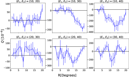
Figure 1: Estimator $Q$ as function of the opening angle $R$ of the patch for all combinations of $\{E_{1},E_{2}\}\in\{10,20,30,40,50\}$ GeV. Patches are centered on $50\leq\varepsilon_{3}\leq 60$ GeV photons with absolute Galactic latitude $|b|\geq 80^{\circ}$; data are from August 2008 through January 2014.

In order to find the parameters upon which the value $Q$ is maximized, we iterate over the following free parameters: the border of the energy bins, the minimally allowed Galactic latitude $b$ for $\varepsilon_{1}$ and $\varepsilon_{2}$ events, and the minimally allowed Galactic latitude of $\varepsilon_{3}$ events. From this analysis, we find that using for the scan eight evenly spaced values with $\varepsilon_{3}$ events at Galactic latitudes $|b|\geq 84^{\circ}$ maximizes the observed value of $Q$: Comparing Fig. 2 to Fig. 1, one can see that the $Q$ values are for some cases much larger in the eight-binned scan.

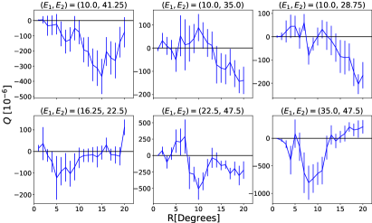
Figure 2: Estimator $Q$ as function of the opening angle $R$ of the patch for some combinations of $\{E_{1},E_{2}\}\in\{10,16,23,29,35,41,48,54\}$ GeV. Patches are centered on $53\leq\varepsilon_{3}\leq 60$ GeV photons with absolute Galactic latitude $|b|\geq 84^{\circ}$; data are from August 2008 through January 2014.

There are currently over 11 years of gamma-ray data available from the Fermi-LAT experiment. Applying the same cuts to this database as were initially applied to the 2014 experiment yields a data set with 29,272 events, whereas the old data set contained only 9,942 events. When the new data set is divided into five evenly spaced energy bins from 10 GeV to 60 GeV (matching the cuts used in Ref. Tashiro et al. (2014)), there are 20,098 events in the 10 GeV energy bin, 5,098 events in the 20 GeV energy bin, 2,252 events in the 30 GeV energy bin, 1,128 events in the 40 GeV energy bin, and 696 events in the 50 GeV energy bin.

Calculating the $Q$ estimator for this data set yields Fig. 3. When comparing Fig. 3 to Fig. 1, it is clear that the $Q$ values obtained for the 2008–2014 data set are unreliable: If the detection would have been real, one would expect to see the signal to grow stronger in the extended data set. However, the $Q$ values are generally a full order of magnitude smaller than those in the smaller data set.

Applying the same analysis of the full data set using the cuts determined from our scan in Fig. 2 yields similar results: There is an order of magnitude decrease in the detected signal when the full data set is analyzed. The results of this analysis are presented in Fig. 4.

We conclude therefore that the hint for helical magnetic fields in the 2.5 year was a fluctuation. In particular, its statistical significance was misinterpreted because the “looking-elsewhere effect” was not accounted for.

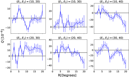
Figure 3: Estimator $Q$ as function of the opening angle $R$ of the patch for all combinations of $\{E1,E2\}\in\{10,20,30,40,50\}$ GeV. Patches are centered on $50\leq\varepsilon_{3}\leq 60$ GeV photons with absolute Galactic latitude $|b|\geq 80^{\circ}$; data are from August 2008 through September 2019.

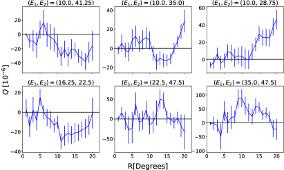
Figure 4: Estimator $Q$ as function of the opening angle $R$ of the patch for some combinations of $\{E1,E2\}\in\{10,16,23,29,35,41,48,54\}$ GeV. Patches are centered on $53\leq\varepsilon_{3}\leq 60$ GeV photons with absolute Galactic latitude $|b|\geq 84^{\circ}$; data are from August 2008 through September 2019.

III Gamma-rays from TeV blazars

In this section, we investigate if extended halos of TeV blazars can be used for the detection of helical magnetic fields. This question was addressed in a series of works using mainly analytical toy models Tashiro and Vachaspati (2013); Tashiro et al. (2014); Tashiro and Vachaspati (2015); Long and Vachaspati (2015); Alves Batista et al. (2016): Neglecting in particular a continuous injection spectrum, fluctuations in the distribution of interaction lengths and the energy distribution of secondaries, it was shown that helical magnetic fields can be detected, if the distance to the source and the correlation length of the turbulent field satisfies certain criteria. Here we use instead of such analytical toy models the version 3.03 of the Monte Carlo program ELMAG Kachelrieß et al. (2012); Blytt et al. (2020) to simulate the three-dimensional evolution of electromagnetic cascades. Replacing in this program the probability distribution functions (pdf) usually employed by their expectation values, we can emulate the analytical toy models used previously. Switching on these sources of fluctuations, we can identify those which affect mostly the detection of helical magnetic fields and understand how large the detection prospects are under realistic assumptions.

If not otherwise specified, we use a source located at the redshift $z=0.25$, corresponding to the comoving radial distance $\simeq 1$ Gpc. We assume as opening angle of the blazar jet $\Theta_{\rm jet}=1^{\circ}$ and inject 10,000 photons into a magnetic field of strength $B_{\rm rms}=10^{-16}$ G. To calculate $Q$, we use photons of energy $10<\varepsilon_{1}/{\rm GeV}<26$ and $74<\varepsilon_{2}/{\rm GeV}<90$ in bins of size $\Delta E=16$ GeV. As EBL model, we choose the one of Gilmore et al. Gilmore et al. (2012).

In order to quantify the detectability of helicity at each stage, we calculate the distribution of $Q$ values for typically $N=500$ Monte Carlo sets. Since we know the position of the source, we adapt the algorithm used in section II slightly, substituting the highest-energy photons $\varepsilon_{3}$, which would only approximate the position of the source, with the actual position of the source. Thus we use only photons produced as secondaries in the cascades for $E_{1}$ and $E_{2}$. Since we do not include background photons in our simulations, it is favorable to use no angular cuts and to include thereby as many photons as possible in the calculation of $Q$.

We find that the probability distribution of $Q$ values is rather well-described by a Gaussian (or normal) distribution, with the deviations increasing as we add more and more sources of physical fluctuations. For each parameter set, we fit two Gaussians $N(\mu_{i},\sigma_{i}^{2})$ to the two distributions of $Q$ values for the right- and left-helical magnetic fields and calculate then their overlap $O$,

$$O=1-\frac{1}{2}\mathrm{erf}\left(\frac{c-\mu_{1}}{\sqrt{2}\sigma_{1}}\right)+\frac{1}{2}\mathrm{erf}\left(\frac{c-\mu_{2}}{\sqrt{2}\sigma_{2}}\right),$$ (2)

where $\mu_{1}<\mu_{2}$ and $c$ is the intersection of the two distributions. When the percentage of overlap between the two distributions is high, positive and negative helical magnetic fields are difficult to distinguish using the $Q$ distribution. Similarly, one can use the overlap to quantify how likely the “signal hypothesis” $|h|=1$ can be distinguished from the “background hypothesis” $|h|=0$.

III.1 Toy model

As a first step, we test the ability to detect with ELMAG magnetic field helicity in the highly idealized scenario adapted from Ref. Long and Vachaspati (2015). In this toy model, photons are injected with a fixed energy $E=10^{13}$ eV. The magnetic field consists of a single mode with helicity $h=\{-1,0,1\}$,

$$\boldsymbol{B}(\boldsymbol{r})=\left(\begin{array}[]{c}B\sin(kz+\beta)\\ hB\cos(kz+\beta)\\ 0\end{array}\right)$$ (3)

and its wave-vector $\boldsymbol{k}$ is pointing along the line-of-sight towards the blazar. Moreover, we replace the pdf for the interaction lengths by their expectation values. Thus the only source of fluctuations in this toy model are the energy fractions transferred to the secondary particles. Finally, we switch off the creation of one charge in the process $\gamma\gamma\to e^{+}e^{-}$ to create by hand a charge asymmetry. We set the observation angle $\Theta_{\rm obs}$ between the line-of-sight and the jet axis to zero.

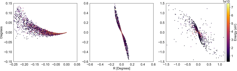
Figure 5: Sky map of the arrival directions of photons: left is the toy model with $L_{\max}=0.1$ Mpc, the middle panel includes both charges and continuous injection spectrum with $L_{\max}=600$ Mpc, and the right is for the realistic case including PDF for interaction lengths, 3D magnetic turbulence and $L_{\max}=600$ Mpc.

In the left panel of Fig. 5, we show the sky map of the arrival directions of photons for $L=2\pi/k=0.1$ Mpc of the magnetic field: A spiral pattern is clearly visible, with the random phase $\beta$ leading only to a rotation of the pattern. Next we estimate the possibility of differentiating between a right and a left-helical IGMF, using as measure the overlap between the probability distributions for the $Q$ values in the two cases. In Fig. 6, we show the Monte Carlo (MC) results together with the fitted normal distributions for various wave-lengths of the single magnetic field mode, from $L=0.1$ Mpc to 100 Mpc, using 500 simulations. The ability to detect a helical IGMF is highly dependent on the wave-length, since the field resembles more and more a uniform one as $L$ increases: As a result, the distance between the peaks of the normal distributions decreases and their overlap increases. Using (3), we calculate an overlap of $1.27\times 10^{-66}$ for a wave-length of $L=0.1$ Mpc, meaning that helicity is perfectly detectable. For $L=1$ Mpc, the overlap of the two peaks is only 19.9%, increasing to 35.2% for $L=10$ Mpc. Finally, the signal for helicity practically disappears for $L=100$ Mpc, where the overlap increases to 93.5%.

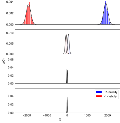
Figure 6: MC results and fitted normal distributions of $Q$ values for the toy model, orange bins for $h=-1$ and blue bins for $h=+1$; the wave-lengths $L$ of the magnetic field mode are, from top to bottom, 0.1 Mpc, 1 Mpc, 10 Mpc, and 100 Mpc.

III.2 Towards the realistic case

III.2.1 Adding continuous injection spectrum

We now modify our highly idealized toy model to include a continuous injection spectrum, but keep otherwise all parameters unchanged. Inspired by high frequency peaked blazars as 1ES 0229+200, we use as injection spectrum the power law $dN/dE_{\rm inj}\propto E_{\rm inj}^{-2/3}$ between $10^{11}\leq E_{\rm inj}\leq 10^{13}$ eV. Including a spectrum of injection energies weakens the correlation between deflection angle and energy, on which the estimator $Q$ is based on. Therefore one may expect that the detection of a helical IGMF becomes more difficult.

In Fig. 7, we show the MC results and the fitted normal distributions of $Q$ values obtained choosing $L=100$, 250, 500, and 750 Mpc for the wave-length of the magnetic field mode (3). Using $N=500$ Monte Carlo simulations, there is no overlap in any case, so that helicity is detectable with a confidence level (C.L.) of at least $99.8\%$. Assuming Gaussian statistics and applying Eq. (2), the C.L. are 99.8% for $L=100$ Mpc, 99.8% for $L=250$ Mpc, 99.8% for $L=500$ Mpc, and 99.7% for $L=750$ Mpc, corresponding to a $3\sigma$ detection using a single source for each case.

These results disagree with the expectation that helicity becomes more difficult to detect using a continuous energy spectrum for the injected photons. The apparent contradiction is resolved noting that the relevant scale to which the wave-length $L$ of the field mode should be compared is the Larmor radius

$$r_{\rm L}=\frac{\gamma mv_{\perp}}{|q|B}$$ (4)

of the produced cascade electrons: It is the dimensionless ratio $L/r_{\rm L}$ which controls if the helical magnetic field appears effectively as a uniform field for the propagating electron. Since the typical energy of these electrons is much lower using a photon injection spectrum extending down to $10^{11}$ eV, the relevant dimensionless ratio $L/r_{\rm L}$ is increased. Thus larger values of $L$ lead in the case of the continuous spectrum to comparable results to the fixed energy case.

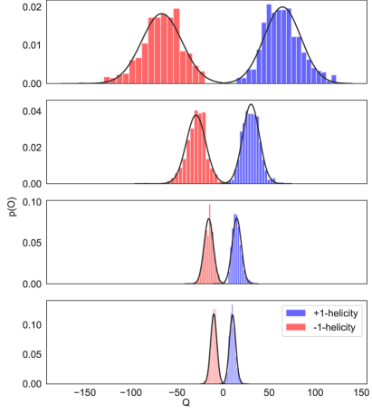
Figure 7: MC results and fitted normal distributions of $Q$ values for toy model at various correlation lengths, orange bins for $h=-1$ and blue bins for $h=+1$. Photons are injected on a continuous spectrum of energies by a source located at 1 Gpc. The correlation lengths for each panel, from top to bottom are: 100 Mpc, 250 Mpc, 500 Mpc, and 750 Mpc. The overlap in each case is approximately 0.

III.2.2 Adding both charges

We continue to use the continuous injection spectrum and the single magnetic field mode (3), but include now both charges created in the process $\gamma\gamma\to e^{+}e^{-}$, thereby removing the artificial charge asymmetry. As a result, helicity cannot be detected when the source is observed directly face on: As shown in the middle panel of Fig. 5, the arrival directions of photons originating from both electron and positron cascades are distributed along anticlockwise spirals in a magnetic field with negative helicity. Thus using photons from either electron or positron cascades leads to a negative contribution to $Q$. By contrast, combining $E_{1}$ and $E_{1}$ photons from an electron and a positron cascade leads to a clockwise spiral as shown in Fig. 8 and, thus, to a positive contribution to $Q$. As a result, the various contributions to $Q$ cancel, leading to a probability distribution consistent with zero helicity, cf. with Fig. 9. The source must therefore be observed off angle, so that either electrons or positrons are deflected preferentially towards the observer.

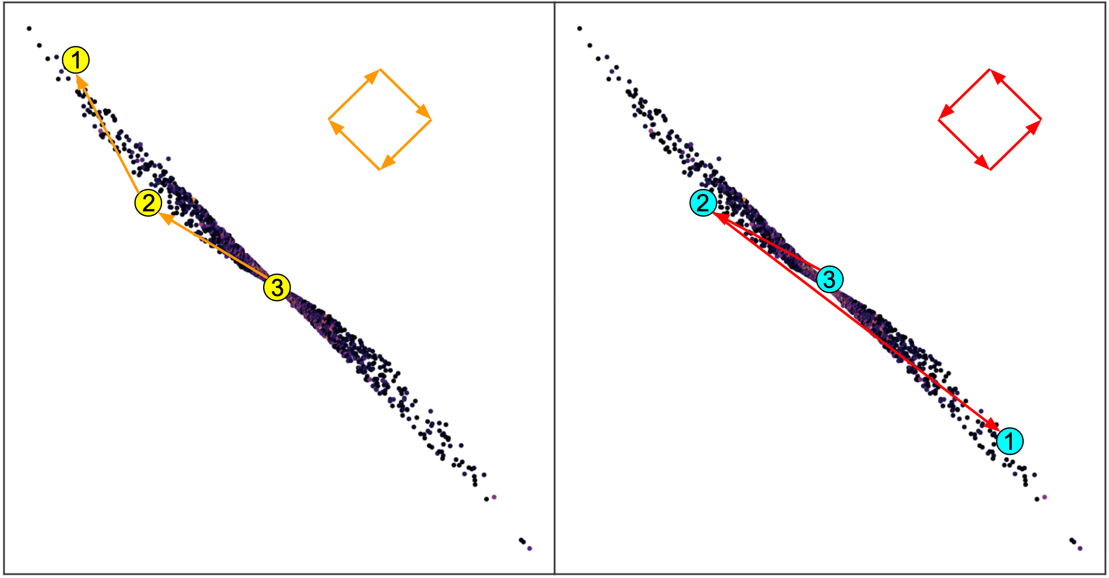
Figure 8: Illustration how the combination of $E_{1}$ and $E_{2}$ photons from an electron and a positron cascade leads to a contribution to $Q$ with the wrong sign.

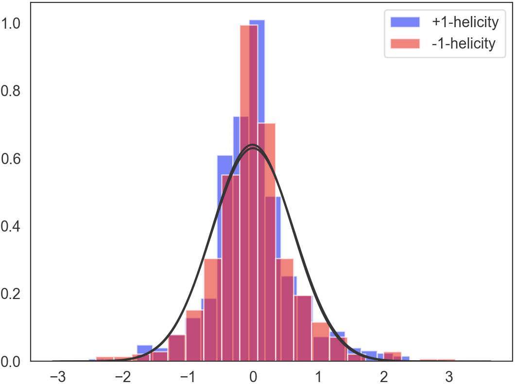
Figure 9: MC results and fitted normal distributions of $Q$ values for the toy model with continuous injection spectrum observed at $\Theta_{\rm obs}=0^{\circ}$, orange bins for $h=-1$, blue bins for $h=+1$, and red for bins with overlap;; The percentage of overlap for the two distributions is 98%.

The bending angle of a cascade under the influence of an IGMF is approximately given by Tashiro and Vachaspati (2013)

$$\Theta(E_{\gamma}) \approx 0.004^{\circ}\biggl{(}\frac{B}{10^{-16}\mathrm{G}}\biggr{)}\biggl{(}\frac{1\mathrm{Gpc}}{D_{s}}\biggr{)}\biggl{(}\frac{E_{\gamma}}{100\mathrm{GeV}}\biggr{)}^{-3/2},$$ (5)

so the size of the source on the sky increases linearly with the strength of the magnetic field. A stronger magnetic field, then, means that there is a larger range of $\Theta_{\rm obs}$ for which helicity can be detected. Therefore, we slightly modify our standard parameters to better highlight the conditions that make detection favorable: We now assume an opening angle for the blazar jet $\Theta_{\rm jet}=2^{\circ}$ and inject photons into a magnetic field of strength $B=10^{-15}$ G.

Increasing the observation angle $\Theta_{\rm obs}$ leads to a stronger signal until a maximum observation angle is reached, beyond which the number of photons detected drops fast. As an example, Fig. 10 shows the $Q$ distributions for a source located at 1 Gpc and observed at $\Theta_{\rm obs}=2.5^{\circ}$, i.e. slightly larger than the jet opening angle $\Theta_{\rm jet}=2^{\circ}$. In this case, one charge is preferentially deflected towards the observer, and as a result, the contributions of cascade electrons and positrons to $Q$ do not cancel out. In this specific case, the overlap between the two distributions is only 8%. In Fig. 11, we show the overlap between the $Q$ distributions for a left- and right-helical fields as function of $\Theta_{\rm obs}$ as blue curve. For small $\Theta_{\rm obs}$, the presence of photons from opposite charge cascades weakens the helicity signal, while for $\Theta_{\rm obs}\raise 1.29167pt\hbox{$\;>$\kern-7.5pt\raise-4.73611pt\hbox{$\sim\;$}}\Theta_{\rm jet}$, the overlap goes to zero. We conclude that, provided that the source is observed at a sufficiently large $\Theta_{\rm obs}$, charges are separated well enough to not destroy the possibility to detect helical magnetic fields.

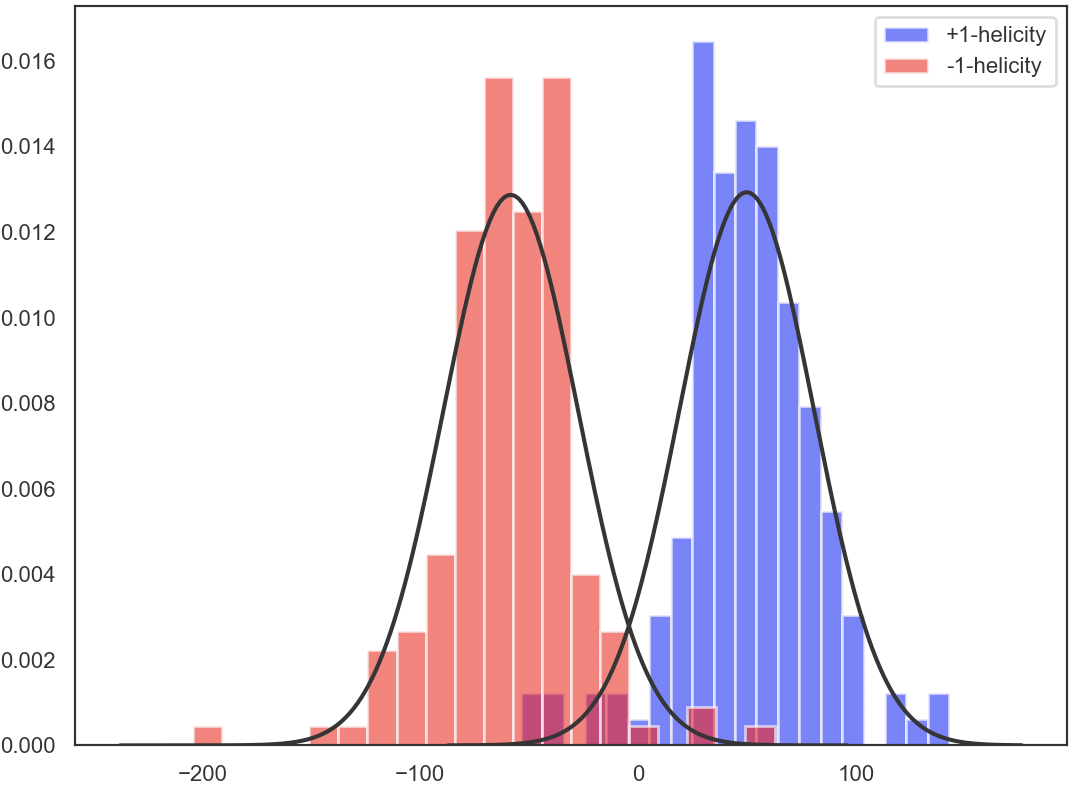
Figure 10: MC results and fitted normal distributions of $Q$ values for a source located at 1 Gpc and observed at $\Theta_{\rm obs}=2.5^{\circ}$, orange bins for $h=-1$, blue bins for $h=+1$, and red for bins with overlap; both charged are included.

Note however that, as $\Theta_{\rm obs}$ increases, it becomes less likely that photons reach the observer. Thus a larger number of sources is needed to produce statistically significant data sets.

III.2.3 Adding fluctuations in the interaction length

Keeping all other properties the same, we now replace the mean-values for the interaction lengths of the reaction $\gamma+\gamma\to e^{+}+e^{-}$ and $e^{\pm}+\gamma\to e^{\pm}+\gamma$ by their pdf’s. Fluctuations in these interaction lengths weaken the relation between the energy and the deflection angle of the observed photons. Therefore we expect that the detection prospects of helical fields will be reduced.

Repeating the previous analysis, we find now that the overlap of the $Q$ distributions shown in Fig. 12 increases from 8% to 47%. The orange curve in Fig. 11 shows the overlap as function of $\Theta_{\rm obs}$ including fluctuations: The signal is considerably weaker, but the same trends are followed until $\Theta_{\rm obs}\approx 2.5^{\circ}$. For $\Theta_{\rm obs}>2.5^{\circ}$, however, the overlap begins to increase again.

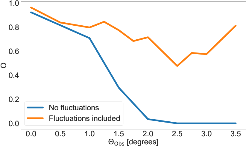
Figure 11: Overlap $O$ as a function of the observation angle $\Theta_{\rm obs}$; the blue curve uses the mean value, the orange curve the pdf’s for the interaction lengths.

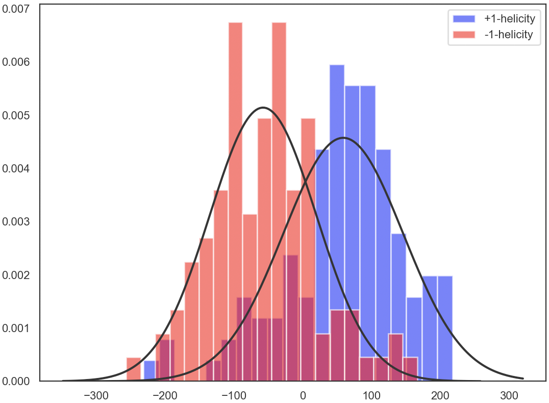
Figure 12: MC results and fitted normal distributions of $Q$ values for a source located at 1 Gpc and observed at $\Theta_{\rm obs}=2.5^{\circ}$ with an opening angle of $\Theta_{\rm jet}=2.0^{\circ}$, orange bins for $h=-1$ and blue bins for $h=+1$; fluctuations in the interaction length are included.

III.2.4 Adding a spectrum of $B$ modes

We now include additional modes of the magnetic fields, but keep all other properties of the simulation the same. The directions of the wave-vectors $\boldsymbol{k}_{i}$ of each mode $i$ are distributed uniformly on the sphere $S^{2}$, while their norm is distributed according to a Kolmogorov power-spectrum. In order to keep the computing times manageable, we use maximally 100 modes. In the right panel of Fig. 5, we show the sky map of the arrival directions of photons for a maximal length of the magnetic field modes $L_{\max}=600$ Mpc: The spiral pattern has become rather fuzzy, indicating that helicity becomes more difficult to detect. The resulting $Q$ distributions are shown for the same parameters as in the previous plot in Fig. 13. The overlap between the $h=+1$ and $h=-1$ pdf’s increases mildly to $\approx 53\%$ and thus including a distribution of field modes does not deteriorates significantly the detection prospects of helical magnetic fields. Also included in Fig. 13 is the distribution for the case that $h=0$, which is as expected centered approximately at $Q=0$. The overlap $O$ between the $h=|1|$ and $h=0$ distribution is $75\%$.

Figure 13: MC results and fitted normal distributions of $Q$ values for a source located at 1 Gpc, observed at $\Theta_{\rm obs}$ = 2.5^∘ with an opening angle of $2.0^{\circ}$, orange bins for $h=-1$, yellow bins for $h=0$, and blue bins for $h=+1$. Photons are injected into a turbulent magnetic field with 100 3D modes.

Let us comment now on the statistical significance, if $N$ such sources are observed. Assuming a Gaussian distribution of the $Q$ values with an overlap of 75%, we can use a Kolmogorov-Smirnov test to estimate the chance probability that for $N$ observations the two distributions are confused: While a $3\sigma$ evidence for helical fields would require $N\simeq 50$ sources, a $5\sigma$ detection would need the observation of $N\simeq 120$ sources with such a signal.

III.2.5 Experimental constraints

We have not taken into account yet constraints like the energy threshold, the finite angular resolution and the limited observation time of specific experiments. While a detailed discussion of these issues is outside the scope of this work, we comment briefly on the case of the Cherenkov Telescope Array (CTA).

The angular resolution of the Southern Array of CTA is estimated to vary between $\ell_{68}=0.05^{\circ}$ at 1 TeV and $0.15^{\circ}$ at 100 GeV, where $\ell_{68}$ denotes the angular opening angle of cone containing 68% of all reconstructed photons Maier et al. (2020). This value is in a considerable part of the relevant $\{B,D_{s}\}$ parameter space comparable to or larger than the extension of the gamma-ray halo given by Eq. (5). Only for magnetic field strengths $B\raise 1.29167pt\hbox{$\;>$\kern-7.5pt\raise-4.73611pt\hbox{$\sim\;$}}10^{-14}$ G, we expect that the spiral patterns contained in the halo of TeV blazars are sufficiently large such that they are not washed out by the finite angular resolution. Another effect deteriorating the detection prospects for helical fields is the reduced sensitivity of CTA below 100 GeV, which requires an adjusting of the energy cuts $E_{1}$ and $E_{2}$.

In order to quantify this effect, we construct the “measured” photon arrival directions from the true ones by adding Gaussian noise with variance $\sigma\simeq\ell_{68}/\sqrt{2.3}$. In Fig. 14, we show for three strengths of the magnetic field the effect of the finite angular resolution of CTA on the measured arrival directions of photons with energy $>100$ GeV. We choose as source distance $D_{s}=1$ Gpc and as wave-length of the magnetic field mode $L=600$ Mpc with 10 turbulent modes. As expected from Eq. (5), the spiral pattern is strongly blurred for $B\raise 1.29167pt\hbox{$\;>$\kern-7.5pt\raise-4.73611pt\hbox{$\sim\;$}}10^{-15}$ G. For $B=10^{-14}$ G, the blurring effect weakens, but is still too strong for magnetic helicity to be detectable, as can be seen in the overlap plots in the bottom of Fig. 14. Increasing the halo size further, the signal-to-background ratio of events would decrease and more detailed studies of specific sources taking into account their luminosity would be needed.

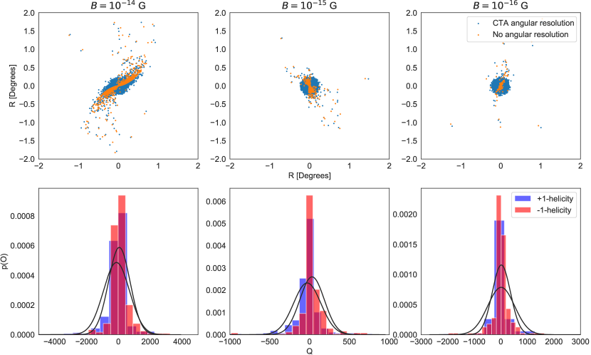
Figure 14: Top panel: Sky map of the arrival directions of photons with $E>100$ GeV for three different magnetic field strengths: orange dots without and blue dots with accounting for the angular resolution. Bottom panel: MC results and fitted normal distributions of $Q$ values, orange bins for $h=-1$ and blue bins for $h=+1$.

IV Conclusions

We have searched for signatures of helical magnetic fields in more than 11 years of gamma-ray data from Fermi-LAT. As expected from general arguments, we have found that this data set composed of diffuse gamma-rays is consistent with zero helicity. We conclude that the hint for helical magnetic fields in the 2.5 year found in Refs. Tashiro et al. (2014); Chen et al. (2015) was a fluctuation, which statistical significance was misinterpreted because the “looking-elsewhere effect” was not accounted for.

We have also examined the detection prospects of non-zero helicity in the IGMF using individual sources as TeV blazars. Starting from a toy model, we have investigated how the addition of realistic features like fluctuations and experimental errors deteriorates the detection prospects. We have found that charge separation can be efficiently achieved by choosing sources with sufficiently large $\Theta_{\rm obs}$. Also the inclusion of a distribution of magnetic field modes does not affect significantly the signal of helical fields. In contrast, fluctuations in the interaction lengths of the reaction $\gamma+\gamma\to e^{+}+e^{-}$ and $e^{\pm}+\gamma\to e^{\pm}+\gamma$ together with a continuous spectrum of injected photon energies weaken the correlation between the energy and the deflection angle of the observed photons and reduce thereby the signal of helical fields considerably. However, if the halos of tens of sources could be observed, a detection is formally still possible.

In order to quantify the detection prospects properly, more detailed investigations taking into account both the specific experimental properties of, e.g., CTA and the expected fluxes of TeV sources are warranted. Additionally, searches for more optimal estimators than the $Q$ statistics are desirable: For instance, likelihood fits of halo templates are on general grounds known to be better, but also less robust, estimators.

Note added

While finalizing this work, the preprint  Asplund et al. (2020) appeared. The authors of Asplund et al. (2020) performed an analysis of the diffuse gamma-ray data from Fermi-LAT including 11 years of data. Their analysis is more detailed than ours and includes also a discussion of several experimental issues of Fermi-LAT. In particular, they estimate the uncertainty of the $Q$ statistics from Monte Carlo simulations, obtaining much larger values than using the method of Ref. Tashiro and Vachaspati (2015). Adding to this finding the “look-elsewhere effect” stressed in this work, the original evidence for helical magnetic fields found in the 2.5 year Fermi data is weakened even more.

References

- Kulsrud and Zweibel (2008) R. M. Kulsrud and E. G. Zweibel, Rept. Prog. Phys. 71, 0046091 (2008), eprint 0707.2783.
- Durrer and Neronov (2013) R. Durrer and A. Neronov, Astron. Astrophys. Rev. 21, 62 (2013), eprint 1303.7121.
- Nikishov (1961) A. I. Nikishov, Zh. Eksperim. i Teor. Fiz. 41, 549 (1961).
- Gould and Schréder (1966) R. Gould and G. Schréder, Phys. Rev. Lett. 16, 252 (1966).
- Berezinsky and Smirnov (1975) V. Berezinsky and A. Smirnov, Astrophys. Space Sci. 32, 461 (1975).
- Strong (1976) A. Strong, J. Phys. A 9, 305 (1976).
- Plaga (1995) R. Plaga, Nature 374, 430 (1995).
- Takahashi et al. (2008) K. Takahashi, K. Murase, K. Ichiki, S. Inoue, and S. Nagataki, Astrophys. J. Lett. 687, L5 (2008), eprint 0806.2825.
- Murase et al. (2008) K. Murase, K. Takahashi, S. Inoue, K. Ichiki, and S. Nagataki, Astrophys. J. Lett. 686, L67 (2008), eprint 0806.2829.
- Aharonian et al. (1994) F. Aharonian, P. Coppi, and H. Voelk, Astrophys. J. Lett. 423, L5 (1994), eprint astro-ph/9312045.
- Neronov and Semikoz (2007) A. Neronov and D. V. Semikoz, JETP Lett. 85, 473 (2007), eprint astro-ph/0604607.
- Dolag et al. (2009) K. Dolag, M. Kachelrieß, S. Ostapchenko, and R. Tomàs, Astrophys. J. 703, 1078 (2009), eprint 0903.2842.
- Elyiv et al. (2009) A. Elyiv, A. Neronov, and D. V. Semikoz, Phys. Rev. D80, 023010 (2009), eprint 0903.3649.
- Neronov et al. (2010) A. Neronov, D. Semikoz, M. Kachelrieß, S. Ostapchenko, and A. Elyiv, Astrophys. J. Lett. 719, L130 (2010), eprint 1002.4981.
- d’Avezac et al. (2007) P. d’Avezac, G. Dubus, and B. Giebels, Astron. Astrophys. 469, 857 (2007), eprint 0704.3910.
- Neronov and Vovk (2010) A. Neronov and I. Vovk, Science 328, 73 (2010), eprint 1006.3504.
- Tavecchio et al. (2010) F. Tavecchio, G. Ghisellini, L. Foschini, G. Bonnoli, G. Ghirlanda, and P. Coppi, Mon. Not. Roy. Astron. Soc. 406, L70 (2010), eprint 1004.1329.
- Dolag et al. (2011) K. Dolag, M. Kachelrieß, S. Ostapchenko, and R. Tomas, Astrophys. J. Lett. 727, L4 (2011), eprint 1009.1782.
- Broderick et al. (2012) A. E. Broderick, P. Chang, and C. Pfrommer, Astrophys. J. 752, 22 (2012), eprint 1106.5494.
- Brandenburg et al. (1996) A. Brandenburg, K. Enqvist, and P. Olesen, Phys. Rev. D 54, 1291 (1996), eprint astro-ph/9602031.
- Olesen (1997) P. Olesen, Phys. Lett. B 398, 321 (1997), eprint astro-ph/9610154.
- Tashiro and Vachaspati (2013) H. Tashiro and T. Vachaspati, Phys. Rev. D 87, 123527 (2013), eprint 1305.0181.
- Tashiro et al. (2014) H. Tashiro, W. Chen, F. Ferrer, and T. Vachaspati, Mon. Not. Roy. Astron. Soc. 445, L41 (2014), eprint 1310.4826.
- Tashiro and Vachaspati (2015) H. Tashiro and T. Vachaspati, Mon. Not. Roy. Astron. Soc. 448, 299 (2015), eprint 1409.3627.
- Long and Vachaspati (2015) A. J. Long and T. Vachaspati, JCAP 1509, 065 (2015), eprint 1505.07846.
- Chen et al. (2015) W. Chen, B. D. Chowdhury, F. Ferrer, H. Tashiro, and T. Vachaspati, Mon. Not. Roy. Astron. Soc. 450, 3371 (2015), eprint 1412.3171.
- Ackermann et al. (2013) M. Ackermann et al. (Fermi-LAT), Astrophys. J. Suppl. 209, 34 (2013), eprint 1306.6772.
- Alves Batista et al. (2016) R. Alves Batista, A. Saveliev, G. Sigl, and T. Vachaspati, Phys. Rev. D94, 083005 (2016), eprint 1607.00320.
- Kachelrieß et al. (2012) M. Kachelrieß, S. Ostapchenko, and R. Tomàs, Comput. Phys. Commun. 183, 1036 (2012), eprint 1106.5508.
- Blytt et al. (2020) M. Blytt, M. Kachelrieß, and S. Ostapchenko, Comput. Phys. Commun. p. 107163 (2020), eprint 1909.09210, URL http://elmag.sourceforge.net/.
- Gilmore et al. (2012) R. Gilmore, R. Somerville, J. Primack, and A. Dominguez, Mon. Not. Roy. Astron. Soc. 422, 3189 (2012), eprint 1104.0671.
- Maier et al. (2020) G. Maier, L. Arrabito, K. Bernlöhr, J. Bregeon, P. Cumani, T. Hassan, J. Hinton, and A. Moralejo (CTA Consortium), PoS ICRC2019, 733 (2020), eprint 1907.08171.
- Asplund et al. (2020) J. Asplund, G. Jóhannesson, and A. Brandenburg, Astrophys. J. 898, 124 (2020), eprint 2005.13065.